electrifying the columbus, - clean natural gas

Electrifying the Columbus,

Ohio Metro Area’s Building

Stock – Economic and Power

Market Impacts

Scott Nystrom

Mitch DeRubis

Ken Ditzel

August 2020

Electrifying the Columbus, Ohio Metro Area’s Building Stock – Economic and Power Market Impacts

2

Table of Contents

Main Takeaways.......................................................................................................................................... 4

Executive Summary ..................................................................................................................................... 5

Methodology and Approach ................................................................................................................... 5

Results ..................................................................................................................................................... 6

Power Market Results ......................................................................................................................... 6

Economic Impact Results .................................................................................................................... 9

Introduction .............................................................................................................................................. 11

Methodology and Approach ..................................................................................................................... 12

Number of New Builds and Conversions .............................................................................................. 12

Assumptions and Inputs for Modeling Conversions ............................................................................. 14

Cost of New Builds and Conversions by Fuel Type ............................................................................... 16

Additional Total Energy and Peak Load ................................................................................................ 17

Building Inputs to the IMPLAN Model .................................................................................................. 19

Residential Customers ...................................................................................................................... 20

Commercial Customers ..................................................................................................................... 22

Electricity Prices ................................................................................................................................ 24

Simulation Results ..................................................................................................................................... 26

Power Market Results ........................................................................................................................... 26

Electricity Load .................................................................................................................................. 26

Capacity Expansion ........................................................................................................................... 29

Electricity Prices ................................................................................................................................ 31

Emissions Results .............................................................................................................................. 34

Economic Impact Results ...................................................................................................................... 36

Macroeconomic Summary ................................................................................................................ 36

Employment Impacts ........................................................................................................................ 37

GDP Contributions ............................................................................................................................ 39

Tax Revenues .................................................................................................................................... 40

Appendix A – Model Diagrams ................................................................................................................. 41

IMPLAN Model Diagram ....................................................................................................................... 41


3

PLEXOS Model Diagram ........................................................................................................................ 41

Appendix B – Load Shapes ........................................................................................................................ 42

Average Residential Customer .............................................................................................................. 42

Average Commercial Customer ............................................................................................................ 43

Appendix C – Capacity Expansion Results ................................................................................................. 44

Base Case .............................................................................................................................................. 44

Electrification – MB Scenario ................................................................................................................ 45

Electrification – RO Scenario ................................................................................................................. 46

Appendix D – Emissions Results ................................................................................................................ 47

Emissions Results – Base Case .............................................................................................................. 47

Emissions Results – MB Scenario .......................................................................................................... 48

Emissions Results – RO Scenario ........................................................................................................... 51

Emissions Results – CO2 in the Base Case, MB Scenario, and RO Scenario ......................................... 54

Emissions Results – NOx in the Base Case, MB Scenario, and RO Scenario ......................................... 55

Emissions Results – SO2 in the Base Case, MB Scenario, and RO Scenario ......................................... 56

Appendix E – IMPLAN Sectoral Aggregation ............................................................................................. 57

Sectoral Aggregation ............................................................................................................................. 57


4

Main Takeaways

• FTI Consulting (“FTI”) modeled the impacts of a policy where all residential and commercial

structures in the Columbus, Ohio metropolitan area (“Columbus MSA”) would install electric

space heating and water heaters, electric cooking and drying equipment, and convert all other

appliances and energy needs from natural gas to electricity.

• According to inputs provided by the American Gas Association (“AGA”), the 20-year cost of

ownership for a representative home with electrical equipment is between $27,200 and

$31,000 – costs with high-efficiency natural gas would be $18,400. For a representative

customer in the commercial sector, the 20-year cost of ownership for electrical equipment

would be $167,200 compared to only $64,200 for gas-fired equipment.

• Converting the Columbus MSA’s building stock to electricity would increase the load for the

power sector, which would lead to slightly higher electricity prices (<1.2% in all years for the

zone home to Columbus). Customers in the Midwest, Appalachia, and the Mid-Atlantic would

face higher prices for electricity. Increased load would engender capacity additions of either 1.2

gigawatts (“GW”) of natural gas combined cycle (“NGCC”) units or, if the incremental builds

must be renewables, then 2.0 GW of photovoltaic solar capacity.

• A critical question is if this policy would reduce emissions and, if so, at what cost. With carbon

dioxide (“CO2”), we project emissions would total 52.9 million metric tons (“MMT”) from 2021

to 2040 when the present fleet of gas-fired equipment sees its replacement by high-efficiency

gas. Electrifying this demand would emit 48.3 MMT in a “market-based” scenario with NGCC

additions or 65.6 MMT in a “renewables-only” scenario with the solar additions, which are 4.6

MMT less (-8.7%) and 12.8 MMT more (24.2%) respectively than baseline.

• For nitrogen oxides (“NOx”) from 2021 to 2040, baseline emissions would be 58,200 short tons.

Market-based emissions would be 10,000 short tons, and renewables-only emissions would be

38,400 short tons.1 For sulfur dioxide (“SO2”) from 2021 to 2040, baseline emissions would be

500 short tons. Market-based emissions would be 5,000 short tons, and renewables-only

emissions would be 38,600 short tons.2 The proposed policy would increase CO2 emissions in

the renewables-only scenario but decrease them in the market-based scenario. The policy

would reduce NOx emissions yet at the cost of higher SO2 emissions.

• The higher costs from electrification for customers in the Columbus MSA would come to $7.4

billion from 2021 to 2040. That market-based scenario would reduce CO2 emissions, but it

would come at a cost of $1,615 per metric ton of saved emissions.

1 Market-based NOx emissions are 82.9% less than baseline NOx; renewables-only is 46.3% less than baseline 2 Market-based SO2 emissions are 908.2% more than baseline SO2; renewables-only is 7,657.0% more than baseline


5

• Using benefit-cost valuations for CO2, NOx, and SO2, the market-based scenario would create

benefits of $377.5 million versus $7.4 billion in costs from 2021 to 2040. At a 5% discount rate,

every $154 in higher costs would produce $1 in benefits. The renewables-only scenario would

be counterproductive because it increases emissions, which translates to $2 billion in additional

costs when monetized. These calculations include only the costs borne by the Columbus MSA

and not the costs borne by customers throughout the region.

• The higher cost of living and higher cost of doing business would have negative implications

within the Columbus MSA’s economy. Consumers, facing higher utility bills and higher costs

passed onto them from commercial establishments, would economize their spending on

consumer staples (e.g., prepared food and retail products).

• By 2040, the Columbus MSA’s economy would have 5,700 fewer jobs and $271 million less in

GDP under electrification compared to a baseline of replacing the existing fleet of gas-fired

equipment with high-efficiency gas through natural attrition. Impacts in the same vein would

continue thereafter because the higher costs would continue.

Executive Summary AGA engaged FTI to examine the potential impacts from converting the housing and commercial

building stocks of the Columbus MSA from natural gas to electricity for their energy needs over the

course of the next 20 years. This report examines the upshot of these conversions on power markets

within Ohio and the Midwest and to the economy of the Columbus MSA.

Methodology and Approach FTI approached this research with three primary tools: (1.) inputs from AGA, (2.) the PLEXOS model,

and (3.) the IMPLAN model. Major inputs from AGA included the number of existing residential homes

and commercial structures to convert plus new builds to adopt either high-efficiency natural gas or

electricity in the next two decades. It also provided the upfront equipment and installation costs and

the long-term maintenance and energy costs for high-efficiency natural gas and electricity and data

describing the seasonal patterns of heating demand for the Columbus MSA.

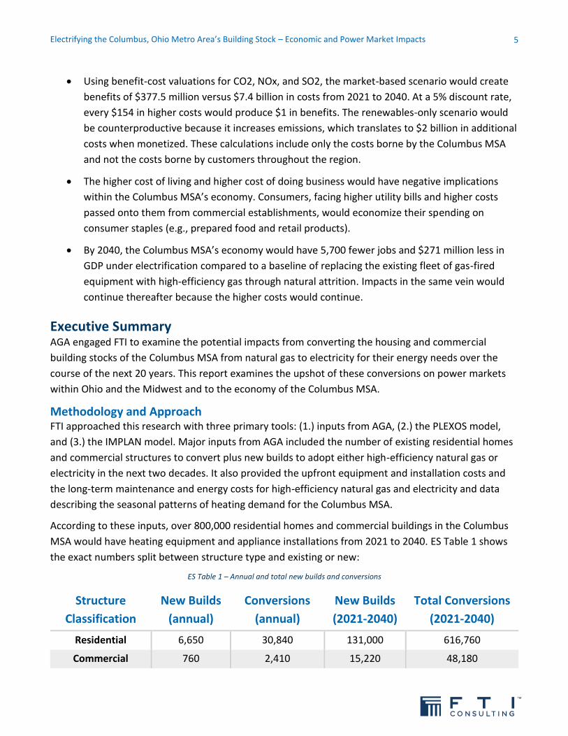
According to these inputs, over 800,000 residential homes and commercial buildings in the Columbus

MSA would have heating equipment and appliance installations from 2021 to 2040. ES Table 1 shows

the exact numbers split between structure type and existing or new:

ES Table 1 – Annual and total new builds and conversions

Structure

Classification

New Builds

(annual)

Conversions

(annual)

New Builds

(2021-2040)

Total Conversions

(2021-2040)

Residential 6,650 30,840 131,000 616,760

Commercial 760 2,410 15,220 48,180


6

The main thrust and driving force behind the results comes from inputs regarding the costs to buy, to

install, and to operate the types of equipment. According to inputs from AGA, the 20-year lifecycle

costs (in 2018 dollars) would be $18,411 for a high-efficiency natural gas home heating system versus

$27,202 to $30,962 for an electric home heating system. The latter range depends on if homes need

updated electric panels to handle higher amperage. For commercial customers, their average costs

over the same period would be $64,240 with gas and $167,160 with electricity.

A net increase in utility bills for residential customers would reduce their purchasing power, which

impacts the local economy and economic sectors dependent on consumer expenditures. The higher

costs for the commercial sector would mean reduced competitiveness or higher costs passed along to

their customers – again negatively affecting households’ purchasing power.

FTI simulated the economic impact of these three effects (more demand for electricity, less demand

for gas, and higher costs) in IMPLAN. IMPLAN is a widely applied model for answering questions on

impacts from policy changes, and a diagram for it is in Appendix A.

The conversion of hundreds of thousands of homes and tens of thousands of commercial structures

over to electric heating systems would increase total and peak electricity load for the Columbus MSA.

To assess these conversions and impacts on wholesale electricity markets in Ohio and the Midwest, FTI

applied its PLEXOS model of the North American electrical system.

PLEXOS determined the impacts on plant additions and plant retirements from the additional load as

well as effects on wholesale prices for the zone encompassing Columbus. FTI integrated the outputs

from PLEXOS for electricity prices into the IMPLAN inputs, as well.

FTI modeled a Base Case without any additional heating electrification and two scenarios in PLEXOS.

For the first scenario, the market could respond to the load without other assumptions or restrictions

(“market-based” or “MB”). In the second scenario, incremental capacity must be solar or wind only

(“renewables-only” or “RO”) without battery storage. The differences between these simulations

produced the change in various types of emissions associated with electrification.

For the remainder of the Executive Summary, we discuss the results of the power market analysis,

results for emissions, and then the results for the economic impact analysis. When then present a

longer narrative and documentation of our inputs and assumptions.

Results Power Market Results

ES Table 2 summarizes the capacity expansion results for the two scenarios. In the MB Scenario, the

increased energy and peak load induces 1.2 GW of NGCC builds relative to the Base Case. In the RO

Scenario, capacity additions would be 2.0 GW of solar. The combination of the higher load and the

operation of these plants would, in turn, influence market prices.


7

ES Table 2 – Capacity expansion from PLEXOS simulations for PJM (2021 to 2040, gigawatts)

Scenario versus

Base Case Sola

r

Win

d

Bio

mas

s

NG

CC

The

rmal

Re

tire

me

nts

Ne

t A

dd

itio

ns

MB Scenario 0.0 0.0 0.0 1.2 0.0 1.2

RO Scenario 2.0 -0.1 0.0 0.0 0.0 1.9

ES Figure 1 shows the electricity price forecast for the American Electric Power (“AEP”) zone in central

Ohio and neighboring states. Electricity prices would remain close to one another but increase in the

MB Scenario and the RO Scenario. The RO Scenario would have the highest prices throughout the

modeling horizon. In MB Scenario, prices are higher only in the 2020s and the late 2030s. The reason is

that the additional NGCC builds in the MB Scenario from ES Table 2 would be flexible resources with

low heat rates and dispatch costs, and hence their dispatch into the market throughout the year would

help to hold average prices down despite the increase in the load.

ES Figure 1 – Annual AEP wholesale electricity price (2018 $)

-0.2%

0.0%

0.2%

0.4%

0.6%

0.8%

1.0%

1.2%

1.4%

$24

$25

$26

$27

$28

$29

$30

$31

$32

20

21

20

22

20

23

20

24

20

25

20

26

20

27

20

28

20

29

20

30

20

31

20

32

20

33

20

34

20

35

20

36

20

37

20

38

20

39

20

40

Per

cen

tage

ch

ange

20

18

$ p

er M

Wh

Base Case MB Scenario ($) RO Scenario ($) MB Scenario (%) RO Scenario (%)


8

We also included inputs related to changing electricity prices (the ones from ES Figure 1) in IMPLAN.

The general effect of affecting households’ purchasing power was the same.

ES Table 3 shows the difference in emissions between the Base Case and the two scenarios. PLEXOS

produces reduces for CO2, NOx, and SO2. Relative to the Base Case, the MB Scenario would reduce

CO2 emissions and the RO Scenario would increase them. Both scenarios would reduce NOx when

compared to the Base Case, though the reduced NOx would come at an increase in SO2 of 4,500 short

tons in the MB Scenario and 38,100 short tons in the RO Scenario.

ES Table 3 – Emissions results (2021 to 2040)

Scenario

CO2 (millions of

metric tons)

NOx (thousands

of short tons)

SO2 (thousands

of short tons)

Base Case 52.9 58.2 0.5

MB Scenario 48.3 10.0 5.0

RO Scenario 65.6 31.3 38.4

MB Scenario versus

Base Case -4.6 (-8.7%) -48.2 (-82.9%) 4.5 (908.2%)

RO Scenario versus

Base Case 12.8 (24.2%) -26.9 (-46.3%) 38.1 (7,657.0%)

For all three compounds, the MB Scenario would have lower emissions than the RO Scenario. Those

results might seem counterintuitive, though they follow from electricity market dynamics. The 1.2 GW

of new NGCC in the MB Scenario would produce emissions, but it would operate at a higher capacity

factor and in more reliably high-load hours than the 2.0 GW of solar in the RO Scenario. NGCC would

therefore be more effective at displacing existing coal generation compared to the incremental solar.

The larger quantities of NOx and SO2 emissions in the RO Scenario relative to the RO Scenario further

demonstrates the solar displaces less coal generation than the NGCC.

ES Table 4 shows the change in emissions from ES Table 3 monetized with federal valuations for CO2

($51 per metric ton), NOx ($6,704 per short ton), and SO2 ($39,599 per short ton).

ES Table 4 – Valuation of the increased or decreased emissions in the scenarios (2018 $ millions)

Scenario CO2 NOx SO2 Total

MB Scenario versus

Base Case $233.1 $323.4 -$179.0 $377.5

RO Scenario versus

Base Case -$649.5 $180.7 -$1,508.8 -$1,977.6


9

The RO Scenario, despite its lower NOx emissions than the Base Case, would have a negative value in

terms of saved emissions because it would increase CO2 and SO2 emissions. Compared to the Base

Case, the MB Scenario would increase SO2 emissions yet decrease CO2 and NOx emissions, which

contributes to its positive overall valuation ($377.5 million) in ES Table 4.

The RO Scenario would be counterproductive towards reducing emissions. The MB Scenario would

achieve emissions reductions, though only at extremely high costs. For the $381.8 million worth of

saved emissions from ES Table 4, customer costs in the Columbus MSA would increase by $7.4 billion

to purchase, install, maintain, and operate electric equipment instead of upgrading to high-efficiency

gas-fired equivalents. These costs are for the Columbus MSA only and do not include higher electricity

prices paid by customers across the Midwest, Appalachia, and the Mid-Atlantic in territories for the

utilities participating in the PJM Interconnection, LLC (“PJM”).

For CO2 alone in the MB Scenario, the cost for the Columbus MSA for the saved emissions from ES

Table 4 would be $1,615 per metric ton. Including NOx and SO2 alongside CO2 and with a 5% discount

rate, every $154 in higher costs would yield $1 in benefits. Most of the emissions reductions in ES Table

4 would come in the 2030s, reducing their present value.

Economic Impact Results

Electrifying residential and commercial building stock would have a negative impact on the economy of

the Columbus MSA over time. The incremental end-consumer expenditures on electricity as compared

to gas expenditures for high-efficiency natural gas heating would gradually reduce expenditures on

other household goods and services. The commercial customers facing the same higher costs would

exacerbate the situation by passing higher costs along to customers.

ES Figure 2 – Economic impact of electrifying the Columbus MSA

-$300

-$250

-$200

-$150

-$100

-$50

$0

-6,000

-5,000

-4,000

-3,000

-2,000

-1,000

0

20

21

20

22

20

23

20

24

20

25

20

26

20

27

20

28

20

29

20

30

20

31

20

32

20

33

20

34

20

35

20

36

20

37

20

38

20

39

20

40

GD

P im

pac

t (2

01

8 $

mill

ion

s)

Emp

loym

ent

imp

act

GDP Employment


10

ES Figure 2 shows results for employment and gross domestic product (“GDP”). As more homes and

structures electrify, the economic impacts would become increasingly negative.

While the aggregate results from ES Figure 2 describe an overall negative impact, the distribution of

those impacts would not be equal across economic sectors.

Electrification would increase the employment associated with the electric power and construction

sectors and decrease the employment associated with natural gas distribution and pipelines. At the

same time, the higher cost of living and the higher cost of doing business due to the electrification

would decrease real incomes and purchasing power across the Columbus MSA, which leads to the

reduced employment for the service sectors in ES Table 5.

ES Table 5 – Employment impact by economic sector

Economic Sector 2025 2030 2035 2040

Electric Power G, T, and D3 240 430 610 770

Construction 90 120 160 180

S&L4 Government (Non-Education) 0 10 10 20

Coal Mining 0 0 0 0

Other Mining 0 0 0 0

S&L Government (Education) 0 0 0 0

Water and Sewage 0 0 0 0

Agriculture and Forestry 0 0 -10 -10

Federal Government -10 -10 -20 -20

Manufacturing -10 -10 -20 -20

Oil and Natural Gas Extraction -10 -20 -30 -40

Information -30 -50 -70 -90

Wholesale -50 -100 -130 -170

Arts, Entertainment, and Recreation -60 -110 -150 -180

Transportation and Logistics -70 -130 -180 -230

Private Education -80 -140 -200 -250

Natural Gas Distribution and Pipelines -160 -290 -410 -510

Other Personal Services -190 -320 -450 -560

Accommodation and Food Service -230 -400 -550 -690

Finance, Insurance, and Real Estate -240 -430 -610 -770

Retail -250 -440 -620 -780

Professional and Business Services -310 -550 -770 -970

Healthcare and Social Assistance -460 -800 -1,100 -1,380

TOTAL -1,830 -3,250 -4,530 -5,710

3 Electric power generation, transmission, and distribution 4 State and local government


11

Introduction The American Gas Association ("AGA") engaged FTI Consulting, Inc. to assess impacts to the Columbus,

Ohio metropolitan area (a 10-county region of central Ohio)5 from electrifying its residential and

commercial building stock, including needs for heating, cooking, and hot water.

According to data from the American Housing Survey (“AHS”),6 most homes in Ohio and by extension

the Columbus MSA use natural gas as their primary heating and cooking fuel. We have examined two

situations for the heating equipment and appliances needs of residential and commercial buildings in

the Columbus MSA. In our “Base Case,” buildings relying on gas in the Columbus MSA would convert to

newer and high-efficiency gas equipment over the next 20 years. Our projected new builds would also

use high-efficiency gas. In our electrification analysis, new builds immediately use electricity for their

heating and appliance needs, and the stock of existing buildings would convert from natural gas to

electricity for their energy needs over the next 20 years.

The electrification would increase higher peak load and total energy in the American Electric Power

(“AEP”) zone of PJM. AEP serves most of the Columbus MSA for its electricity demand. We used a

model of the system called PLEXOS to examine what the load would mean for wholesale electricity

markets under two scenarios. In the “Market-Based Scenario,” the electricity market could add any

type of generation making economic sense to serve higher load. In the “Renewables-Only Scenario,”

we restricted any incremental additions to solar and wind plants only.

Figure 1 organizes the Base Case and our two scenarios for the electricity market modeling.

Figure 1 – Summary of the scenarios for analysis

5 A 10-county region of central Ohio including Delaware, Fairfield, Franklin, Hocking, Licking, Madison, Morrow, Perry, Pickaway, and Union Counties 6 “American Housing Survey,” U.S. Census Bureau, https://www.census.gov/programs-surveys/ahs.html

Analysis Pathways

Base CaseElectrification

Scenarios

Market-Based ("MB")

Scenario

Renewables-Only ("RO")

Scenario

https://www.census.gov/programs-surveys/ahs.html


12

The main body of this report describes the Base Case, scenarios, their inputs, and their assumptions

with additional details. We then describe the impacts of electrifying the Columbus MSA’s residential

and commercial building stock with the results from simulations in PLEXOS and IMPLAN.7 IMPLAN is an

“input-output” model of regional economies designed to show the impacts of changes to economies

and public policy. Where appropriate, we have included appendices with more detailed data tables

documenting our results and describing PLEXOS and IMPLAN.

Methodology and Approach AGA provided the inputs and assumptions underlying the FTI simulations in PLEXOS and IMPLAN.8 AGA

based its analysis on federal and regional data sources, such as the U.S. Census Bureau, and previous

research on the relative cost and efficiency of natural gas-fired appliances and heating equipment

relative to using electricity-powered alternatives for the same purposes.

Number of New Builds and Conversions The first major consideration across the analysis was the number of homes and commercial buildings

to convert to high-efficiency gas (in the Base Case) or electricity (under electrification). On top of these

are new homes and structures being built, which could have either high-efficiency gas (in the Base

Case) or electricity (in the two electrification scenarios). Table 1 describes our inputs for new builds

and conversions annually and for the next 20 years.

Table 1 – Annual and total new builds and conversions

Structure

Classification

New Builds

(annual)

Conversions

(annual)

New Builds

(2021-2040)

Total Conversions

(2021-2040)

Residential 6,650 30,840 131,000 616,760

Commercial 760 2,410 15,220 48,180

We chose 20 years as our horizon because it is a reasonable estimate of the service life for equipment

of this nature. We are not analyzing any “early” conversions and instead assume upgrades to new gas

or electrified equipment comes as the existing fleet naturally turns over.

The Base Case and scenarios would require the conversion of 616,760 homes and 48,180 commercial

buildings over the course of 20 years, which are estimates of the size of the stock for the Columbus

MSA in 2020. These conversions would proceed in a linear fashion with 5% of the initial total having

conversion each year. On top of these would be 6,650 residential new builds and 760 commercial new

builds each year, eventually adding to the aggregate totals in Table 1.

7 “Where It All Started,” IMPLAN, https://implan.com/history/ 8 For diagrams of PLEXOS and IMPLAN, please see Appendix A

https://implan.com/history/


13

In addition, many older homes would require upgrades to their electrical panel to handle the electric

heating equipment and appliances imagined under electrification. Our estimate is 32% of older homes

(the ones built before 1960) in the Columbus MSA would require these upgrades. The plan for the

electrification would require that 9,870 homes year and 197,360 overall homes from 2021 to 2040

would require modernizing their panel to higher amperage.

Figure 2 shows a graphical representation of the data from Table 1 for residential structures. Figure 3

displays the equivalent data but for commercial structures. Under both situations, existing structures

begin with gas-fired equipment at present efficiency. For the Base Case, existing structures would

convert to new, high-efficiency gas equipment over time. New builds would also come online with

high-efficiency gas equipment. For the electrification, the conversions and new builds would instead

come up to speed with electrified equipment and appliances.

Figure 2 – Existing residential structures, conversions, and new builds (thousands)

Figure 3 – Existing commercial structures, conversions, and new builds (thousands)

0

100

200

300

400

500

600

700

800

2020 2021 2022 2023 2024 2025 2026 2027 2028 2029 2030 2031 2032 2033 2034 2035 2036 2037 2038 2039 2040

Existing Unconverted Existing Converted New Builds

0

10

20

30

40

50

60

70

2020 2021 2022 2023 2024 2025 2026 2027 2028 2029 2030 2031 2032 2033 2034 2035 2036 2037 2038 2039 2040

Existing Unconverted Existing Converted New Builds


14

Assumptions and Inputs for Modeling Conversions AGA provided FTI with inputs and assumptions for the cost of new gas-fired equipment, the cost of

new electrical equipment, and the ongoing energy costs to operate them.

The AGA model of residential and commercial natural gas customers is derived from the U.S. Energy

Information Administration (“EIA”) and its data sources, including its monthly consumption and its

customer count data for 2018. Using these sources, AGA estimated a space heating load by subtracting

the average summer consumption from total annual consumption. Hourly heating load data comes

from allocating the monthly demand load by hourly heating degree data.

Limiting the input data to 2018 was a deliberate choice. That year had nominal winter weather both

locally and nationally compared to 30-year heating degree day averages. Additionally, by using a single

year for reference instead of a long-term average the peak of the peak energy demand for the coldest

hours of the year would be present in the shape data. Preserving this facet of the shape helps provide

the electricity sector modeling with more realistic conditions.

Heat pump performance on the handbook produced by the American Society of Heating, Refrigerating,

and Air-Conditioning Engineers (“ASHRAE”). This analysis assumes a nameplate efficiency of 300% at

35°F and a maximum output of 100% of the demand load. The maximum output and the efficiency at

35°F can increase though only by oversizing the unit and thereby increasing costs to consumers paying

to purchase, install, maintain, and operate the unit.

To account for a wider range of air compressor abilities, if the outdoor air temperature remained

above -27°F, the heat pump would continue to function. However, its performance and its maximum

output would decrease as the temperature drops from -35°F. These assumptions are consistent with

the ASHRAE handbook for heat pump operations. The model determined approximately 25% of space

heating demand comes from backup resistance. The model also determined the actual efficiency for

modeled representative heat pumps in the Columbus MSA to be 230%.

Customers converting to heat pumps would install a 300% rated unit in exchange for a retired 80%

efficient gas-fired unit along with a heat pump water heater and all-electric appliances. The baseload

appliance performance derived from a regional weighted average developed using RECS 20159 and

CBECS 201210 surveys. AGA found the average residential customer has a baseload efficiency of 73%

and the average commercial customer has a baseload efficiency of 72%.

For residential customers, AGA assumed the average efficiency of heat pump water heaters had a

minimum rating of 200% and, on average, all non-space heating appliances fit a profile of 178%. For

9 “2015 Residential Energy Consumption Survey,” U.S. Energy Information Administration, https://www.eia.gov/consumption/residential/data/2015/ 10 “2012 Commercial Buildings Energy Consumption Survey,” U.S. Energy Information Administration, https://www.eia.gov/consumption/commercial/data/2012/

https://www.eia.gov/consumption/residential/data/2015/

https://www.eia.gov/consumption/commercial/data/2012/


15

commercial customers, who have much greater needs for water heating and baseload, AGA used a

conversion profile of 125% efficiency compared to a gas equivalent.

Table 2 and Table 3 summarize these inputs. Because commercial customers have widely diverging

requirements for space heating capabilities, AGA did not evaluate the installation costs between gas

furnaces and electric heat pumps for the commercial customer segment.

Table 2 – Summary of assumptions and inputs for residential conversions

De

man

d C

ate

gory

Equ

ipm

en

t Ty

pe

Effi

cien

cy

An

nu

al S

ite

En

ergy

(MM

Btu

)

An

nu

al F

ue

l Co

sts

(20

18

$)

Inst

alla

tio

n C

ost

s

(20

18

$)

Equ

ipm

en

t C

ost

s

(20

18

$)

Space Heating Gas Furnace 80% 70.3 $460 $1,600 $4,026

Space Heating Gas Furnace 96% 58.6 $383 $1,903 $4,788

Space Heating Heat Pump 300% 24.7 $717 $2,224 $4,158

Baseload Gas Furnace 73% 16.4 $203 - -

Baseload Heat Pump 178% 6.7 $249 - -

Table 3 – Summary of assumptions and inputs for commercial conversions

De

man

d C

ate

gory

Equ

ipm

en

t Ty

pe

Effi

cien

cy

An

nu

al S

ite

En

ergy

(MM

Btu

)

An

nu

al F

ue

l Co

sts

(20

18

$)

Space Heating Gas Furnace 80% 480.0 $2,284

Space Heating Gas Furnace 96% 400.0 $1,904

Space Heating Heat Pump 300% 169.7 $4,371

Baseload Gas Furnace 72% 243.5 $1,308

Baseload Heat Pump 125% 142.2 $3,987


16

Cost of New Builds and Conversions by Fuel Type Table 4 describes this input data for the residential sector. We have divided these costs between the

“equipment costs” for the physical equipment, “installation costs” for the labor associated with setting

them up, and “energy costs” for the cost of the natural gas or the electricity to operate the equipment

and maintain it for one year. The numbers in Table 4 include the heating costs and the baseload costs

associated with other activities, such as heating water.

Table 4 – Input costs and assumptions for residential conversions (2018 $)11

Type of Equipment Equipment

Costs

Installation

Costs

Energy

Costs12

Total Costs

(2021-2040)13

Existing Gas - - $663 -

High-Efficiency Gas $4,788 $1,903 $586 $18,411

Electrification $4,158 $2,224 $1,041 $27,202

Electrification

(older homes) $7,91814 $2,22415 $1,041 $30,962

Replacing existing gas equipment at fleet average efficiency with new, high-efficiency gas equipment

would save on energy costs but requires the equipment and installation costs in Table 4. All homes in

the Columbus MSA, however, must upgrade between 2021 and 2040 because of our 20-year horizon

and 20-year assumption of the useful lifespan of the equipment.

When developers build a new home or an existing home needs to replace its equipment, the choice is

between high-efficiency gas and electrification. Electrification would have higher energy costs and

higher installation costs, though the cost of equipment would be lower for newer homes. For the 32%

of older homes built before 1960 requiring additional upgrades, the equipment costs for choosing

electrification would also be higher than new gas. With an example new build or conversion in early

2021, the 20-year cost for the new gas customer is $18,411 and the 20-year cost for electrification is

either $27,202 for newer homes or $30,962 for older homes.

Differences in the costs for customers over the age of the equipment – between $8,800 and $12,500

depending if an electric panel upgrade is required – would be a force behind the economic impact of

11 Assumptions regarding installation costs for natural gas and electric air-sourced heat pump systems imported from, “Implications of Policy-Driven Residential Electrification,” American Gas Association, 5 September 2018, https://www.aga.org/research/reports/implications-of-policy-driven-residential-electrification/ 12 Includes the annual and ongoing costs of both energy and maintenance 13 Equipment costs, plus installation costs, plus energy costs times 20 – representative of a conversation from 2021 only because conversions from subsequent years would have less than 20 years of energy costs 14 Cost to upgrade the water heater branch circuit and electrical panel to higher amperage 15 Assumed to be the same as for newer homes

https://www.aga.org/research/reports/implications-of-policy-driven-residential-electrification/


17

electrifying the home and building stocks. Residential customers would have overall higher utility bills

with electrification relative to the Base Case. This forces households to economize their spending on

the other fixtures of life, such as retail spending or prepared food. Figure 2 illustrates the size of this

effect increases over time as more and more homes come online or convert.

Table 5 summarizes our inputs for commercial buildings. For this sector, we have assumed equipment

and installation costs are the same between new high-efficiency gas and electrification. All differences

in costs for this sector would be, therefore, based on energy costs alone. There is no special carveout

for older commercial structures to upgrade their electrical panels.

Table 5 – Input costs and assumptions for commercial conversions (2018 $)16

Type of Equipment Energy

Costs

Total Costs

(2021-2040)

Existing Gas $3,592 -

High-Efficiency Gas $3,212 $64,240

Electrification $8,358 $167,160

As is the case with residential customers, the difference in lifecycle costs for commercial customers in

Table 5 would be a driving factor in the impact of electrifying the Columbus MSA. For the average

commercial conversion or new build in early 2021, their costs under electrification would be $102,920

than in the Base Case when using high-efficiency gas.

Facing higher utility bills after electrification of their equipment, commercial enterprises would need to

economize as much as residential customers. We have modeled this through a mixture of passing

those higher costs along to their customers in the Columbus MSA and reducing their output because

high costs reduces their competitiveness on national markets.

Additional Total Energy and Peak Load AGA also provided FTI with data on the increase in electricity load likely under the electrification. This

includes an hourly “load shape” for the average customer by type17 and the average baseload.18 The

16 Assumptions regarding installation costs for natural gas and heat pump systems imported from, “Implications of Policy-Driven Residential Electrification,” American Gas Association, September 2018, https://www.aga.org/research/reports/implications-of-policy-driven-residential-electrification/ 17 Average residential and commercial space heating and general non-space heating load derived from monthly natural gas consumption data and the Ohio customer count for 2018, “Natural Gas Consumption,” U.S. Energy Information Administration, https://www.eia.gov/naturalgas/data.php#consumption 18 Monthly non-space heating demand determined as the average consumption per Ohio customer in the months of July and August using the Residential Energy Consumption Survey, and an average natural gas customer profile created to convert that demand into general load, “Residential Energy Consumption Survey 2015,” U.S. Energy Information Administration, https://www.eia.gov/consumption/residential/index.php and, “Commercial Buildings Energy Consumption Survey 2012,” U.S. Energy Information Administration, https://www.eia.gov/consumption/commercial/

https://www.aga.org/research/reports/implications-of-policy-driven-residential-electrification/

https://www.eia.gov/naturalgas/data.php#consumption

https://www.eia.gov/consumption/residential/index.php

https://www.eia.gov/consumption/commercial/


18

baseload occurs across all hours of the year while the hourly shape represents the hourly and seasonal

variations in energy demand for heating and other requirements. AGA analyzed weather data from

201819 and a heating degree days methodology to determine the shape.20

Our input baseload for the average residential customer was 1,974 kilowatt-hours (“kWh”) per year, or

0.23 kWh in any given hour. For the average commercial customer, our input for their annual baseline

was 41,709 kWh, or 4.76 kWh of baseload for any given hour of the year. The analysis here does not

address the potential for electrification in the industrial sector.

Figure 4 shows the load shape for the average residential customer from the AGA data. The shape

implies the load from electrified homes would be at their lowest during the summer months of June,

July, August, and into September, which have little heating load.

Figure 4 – Hourly load shape for the average residential customer (kWh)

The load for heating begins to appear in October and November, peaks in January, and decreases

throughout the rest of the late winter and early spring with numerous oscillations along the way to

account for daily and weekly temperature variations in Ohio.

Figure 5 has the same data for commercial customers. The trends between Figure 4 and Figure 5 are

generally similar. Summer load from electrified commercial customers is at its nadir, and it is usually

the same as the baseload. Heating load becomes a factor in October and November, again peaks in

19 Monthly space heating load weighted by local hourly weather data from the National Centers for Environmental Information (“NOAA”), https://www.ncdc.noaa.gov 20 FTI added 7% to the AGA data to account for transmission and distribution losses

0

1

2

3

4

5

6

7

8

9

10

Jan-18 Feb-18 Mar-18 Apr-18 May-18 Jun-18 Jul-18 Aug-18 Sep-18 Oct-18 Nov-18 Dec-18

https://www.ncdc.noaa.gov/


19

January, and slowly decays throughout the first half of the year to May. Despite the straightforward

seasonal patterns of the additional load, there are complex and seemingly random fluctuations for

hourly and daily load data because of varying temperatures.

Figure 5 – Hourly load shape for the average commercial customer (kWh)

Appendix B summarizes the average electricity load by month and hour for the two customer types.

Table 11 covers residential customers, and Table 12 covers commercial customers.

FTI used the load shapes in Figure 4 and Figure 5 as well as the conversions and new builds detailed in

Figure 2 and Figure 3 to estimate the additional load on an hourly basis from the start of 2021 through

to the end of 2040. First, for any given years, FTI multiplied the load shapes by the sum of all previous

conversions and new builds from previous years. Second, we added to that with new conversions and

new builds from the present year while assuming the present year’s load came online throughout the

year linearly (i.e., without season trends). Third, we added this incremental load to the electrification

scenarios on top of the preexisting load for AEP in the PLEXOS model.21

Building Inputs to the IMPLAN Model We used the information from the previous subsections to build inputs into the IMPLAN model to

simulate the economic impacts of electrification on the Columbus MSA. The inputs represent the net

21 The heat pumps have a theoretical coefficient of performance of 3.0 and a space heating operating range between 65°F and -27°F. The optimal breaking point was assumed to be 35°F, which would suggest each unit was properly sized to fit the ASHRAE Handbook description for heat pump installation, 2016 ASHRAE Handbook, HVAC Systems and Equipment, Chapter 49, p. 10, Figure 13, “Operating Characteristics of Single-State Unmodulated Heat Pump”

0

10

20

30

40

50

60

70

80

Jan-18 Feb-18 Mar-18 Apr-18 May-18 Jun-18 Jul-18 Aug-18 Sep-18 Oct-18 Nov-18 Dec-18


20

difference between the Base Case and the electrification scenarios. We simulated the results on an

annual basis starting in 2021 and concluding at the end of 2040.

Residential Customers

For residential customers, our inputs into IMPLAN take the form of six categories. Those categories

include those from Table 4 as well as some additional details:

1. Equipment Spending

2. Installation Spending

3. Maintenance Spending

4. Natural Gas Spending

5. Electricity Spending

6. Consumption Reallocation

“Consumption reallocation” is the money available to residential consumers that they could spend on

their own preferences in one scenario but cannot in another because of higher costs. Table 4 shows

the electrification of homes would require residential customers to spend more of their incomes on

energy-related bills (including #1 through #5 on the list) compared to the Base Case with its lower

overall costs. The difference is the consumption reallocation.

Because of the consumption reallocation, households would reallocate their spending away from daily

needs for goods and services at the margin. Instead, they would use that same money to cover higher

energy-related costs. Such an approach assumes consumers’ price elasticity of demand for energy

needs is perfectly inelastic. One of the main economic impacts of electrifying the Columbus MSA is the

effect that this reallocation has on the economic sectors depending on consumers in the region, such

as retail, healthcare, food services, and arts and entertainment.

The following list summarizes how FTI inputted each of these as inputs into IMPLAN:

1. Equipment Spending – We inputted net changes in equipment spending by year as added or

reduced demand for the relevant manufacturing sectors for gas-fired heating equipment, for

electric heat pumps, and for electrical panels. We assumed retrofitting homes would pay for

the difference in costs in the immediate year. For new homes, we assumed the difference in

costs become part of the purchase price of the home. Hence, we amortized any difference in

costs across 30 years of payments. We estimated the interest rate attached to 30-year fixed

mortgages in the future based on data from the Congressional Budget Office (“CBO”)22 and

from the Federal Reserve. CBO projects the interest rate for 10-year U.S. Treasury Notes from

22 “The Budget and Economic Outlook: 2020 to 2030,” Congressional Budget Office, 28 January 2020, https://www.cbo.gov/publication/56020

https://www.cbo.gov/publication/56020


21

2021 through 2030,23 which we extended by assuming the rate for 2030 (3.1%) remains the rate

through 2040. We then analyzed the historical difference between interest rates on 10-year

U.S. Treasury Notes24 and 30-year fixed mortgages.25 We found the difference between the two

was 1.76% on average over the past 20 years. We applied this difference to the extended CBO

forecast to generate a forecast of mortgage rates out through 2040.

2. Installation Spending – We inputted net changes in installation spending by year through

demand for the relevant construction and maintenance sectors in IMPLAN. We applied similar

assumptions to these inputs as the ones for equipment spending – installation costs for new

homes become part of the purchase price, and the costs are part of amortizing the price of the

structure. Retrofits are considered a cost in the immediate year.

3. Maintenance Spending26 – For maintenance, we entered net changes in spending by year by

changing demand for the relevant construction and maintenance sectors in IMPLAN. We

assumed maintenance spending is a cost in its immediate year.

4. Natural Gas Spending – We entered the net changes in natural gas spending – which was a

reduction when moving from the Base Case to the electrification scenarios – as a decrease in

demand for the natural gas distribution sector in IMPLAN. The gas distribution sector in IMPLAN

includes local gas utilities and, through the input-output linkages inherent within the model, it

links into natural gas pipelines and extraction.

5. Electricity Spending – We entered the net changes in electricity spending as a decrease in the

demand for the electric power transmission and distribution sector in IMPLAN. Such spending

increased in the electrification scenarios relative to the Base Case, and we considered energy

expenditures as something covered in their immediate year.

6. Consumption Reallocation – For any given year, we entered the opposite number as the sum of

the other five factors as consumption reallocation. For instance, if for each year the net effect

regarding the sum of the costs for the other five factors was $2,000, then we reallocated the

level of household consumption by -$2,000 in IMPLAN. We used the underlying consumption

equation in IMPLAN to determine which economic sectors would experience a decrease in their

demand through the apportionment of the consumption reallocation.

Figure 6 provides an example of the IMPLAN inputs for the residential sector in 2040. Spending for

equipment would be slightly higher ($4 million) in the Base Case, though higher expenditures for

23 “10-Year Economic Projections,” Congressional Budget Office, 28 January 2020, https://www.cbo.gov/system/files/2020-01/51135-2020-01-economicprojections_0.xlsx 24 “10-Year Treasury Constant Maturity Rate,” Federal Reserve Economic Data, https://fred.stlouisfed.org/series/DGS10 25 “30-Year Fixed Rate Mortgage,” Federal Reserve Economic Data, https://fred.stlouisfed.org/series/DGS10 26 Considered separately here and in the inputs to the IMPLAN model even if combined with the ongoing expenditures for energy/operations in Table 4

https://www.cbo.gov/system/files/2020-01/51135-2020-01-economicprojections_0.xlsx

https://www.cbo.gov/system/files/2020-01/51135-2020-01-economicprojections_0.xlsx

https://fred.stlouisfed.org/series/DGS10

https://fred.stlouisfed.org/series/DGS10


22

installation and maintenance in the electrification scenarios mean cost for equipment and labor would

be higher ($66 million) in that scenario. The lion’s share of the difference in costs between the

situations comes from energy costs. In the Base Case, the residential sector spends $439 million on

natural gas compared to $726 million when under electrification.

The difference in total expenditures between the two – which is $354 million – becomes the data for

the consumption reallocation in Figure 6. Household consumers in the Base Case would have more

leftover income to spend on their typical needs and wants.

Figure 6 – IMPLAN inputs for 2040 for the residential sector (2018 $ millions)

Commercial Customers

The process for building IMPLAN inputs related to commercial customers was like the approach for

residential customers. However, there were two important differences:

1. We assumed equipment costs, installation costs, and maintenance costs were the same for

commercial customers between the Base Case and the electrification scenarios (as we earlier

described in Table 5). Hence, there was no need to consider if commercial customers would

amortize their costs over a 30-year loan period, and we assumed they covered their higher

costs for electricity relative to natural gas in the immediate year.

2. FTI treated the equivalent concept to “consumption reallocation” for commercial customers

differently than we did for residential customers, which we document here.

Under the electrification scenarios, commercial customers would have higher energy costs than they

would under the Base Case. We need to reflect these higher costs in the IMPLAN model, though

$0 $200 $400 $600 $800 $1,000 $1,200

Base Case

Electrification

Base Case Electrification

Equipment Spending $187 $183

Installation Spending $74 $87

Maintenance Spending $0 $57

Natural Gas Spending $439 $0

Electricity Spending $0 $726

Consumption Reallocation $354 $0


23

commercial customers are not like households where they would simply reduce their consumption on

the margin like households would when paying higher utility bills.

We have modeled this reallocation in IMPLAN through two paths. For the share of each commercial

sector’s business done within the Columbus MSA,27 we have assumed they pass the same proportion

of their higher costs along to customers within the Columbus MSA. For instance, IMPLAN estimates

76.4% of hospital activities28 in the Columbus MSA are for consumers in the Columbus MSA with the

remainder (24%) “exported” to customers outside the Columbus MSA.

We consider the 76.4% estimate from IMPLAN reasonable for three reasons. First, it is lower than the

other healthcare sectors (such as ambulatory care). Other healthcare sectors in the Columbus MSA

derive more than 95% of their business from the Columbus MSA, which is sensible when patients in

need of ambulatory services are more likely to seek services close to home. Second, the 76.4% figure is

much higher than sectors that purely depend on exports. For instance, sectors such as hotels generate

less than 5% of their business from local customers in IMPLAN.

Our third reason is the most notable and requires additional context. The Columbus MSA has a large

healthcare sector that services not just local customers but also the surrounding rural areas, the rest of

Ohio, and even other states. Example institutions include the Ohio State University’s Wexner Medical

Center,29 OhioHealth, Mount Carmel Health System,30 and Nationwide Children’s Hospital. Each of

these institutions employs thousands and has multiple facilities. All rank among the largest employers

in the Columbus MSA along with the state of Ohio.31 Thus, IMPLAN illustrating the economy and the

healthcare system of the Columbus MSA as “most” (76.4%) of inpatients are from the Columbus MSA

with 24% of inpatients from the surrounding region is reasonable.

For the share of higher energy costs attributed to exports, we have reduced the direct outputs of

commercial sectors themselves. Higher costs for businesses in the Columbus MSA would degrade their

competitiveness relative to the other options in the regions for consumers. For instance, to continue

with the example of hospitals, their higher energy costs to provide inpatient care would discourage

patients and insurance companies from the regions outside of the Columbus MSA from using their

services. Instead, nonlocal patients could instead choose to utilize local facilities or similarly renowned

facilities in Cincinnati, Cleveland, Pittsburgh, or southeast Michigan.

27 IMPLAN calls this the “local use ratio” or the “regional supply coefficient,” the “RSC” 28 NAICS 622, “Industries in the Hospitals subsector provide medical, diagnostic, and treatment services that include physician, nursing, and other health services to inpatients and the specialized accommodation services required by inpatients, https://www.census.gov/cgi-bin/sssd/naics/naicsrch?code=622&search=2017%20NAICS%20Search 29 “About Us,” The Ohio State University Wexner Medical Center, https://wexnermedical.osu.edu/about-us 30 “About Us,” Mount Carmel, https://www.mountcarmelhealth.com/about-us/ 31 Robin Smith, “Here are Central Ohio’s largest employers: Our rankings found 120+ organizations with 100+ workers,” Columbus Business First, 12 July 2019, https://www.bizjournals.com/columbus/news/2019/07/12/here-are-central-ohios-largest-employers-our.html

https://www.census.gov/cgi-bin/sssd/naics/naicsrch?code=622&search=2017%20NAICS%20Search

https://wexnermedical.osu.edu/about-us

https://www.mountcarmelhealth.com/about-us/

https://www.bizjournals.com/columbus/news/2019/07/12/here-are-central-ohios-largest-employers-our.html

https://www.bizjournals.com/columbus/news/2019/07/12/here-are-central-ohios-largest-employers-our.html


24

Figure 7 shows an example flowchart of this process for the hospital sector. The process is similar in all

other commercial sectors within the IMPLAN model.32

Figure 7 – Calculation process in 2040 for the hospital sector

1. Increase in energy costs for all commercial customers = $326.3 million

2. Hospitals’ share of all commercial customers’ natural gas demand in IMPLAN = 3.2%

3. Increase in hospitals’ energy costs in 2040 = $10.5 million33

4. Share of hospitals’ customers coming from the Columbus MSA = 76.4%

5. Higher costs passed along to local customers in the Columbus MSA = $8.0 million

a. Add these costs to the “consumption reallocation” from the previous section

b. Similar effects to economic sectors depending on consumer expenditures

6. Costs borne by hospitals as reduced output from reduced competitiveness = $2.5 million

We repeated a similar set of calculations for all commercial sectors in the IMPLAN model for all years,

which we then inputted into the model for our simulations.

Electricity Prices

We also modeled the impacts of higher electricity prices in IMPLAN. As described, the electrification

scenarios would engender additional electricity load in PJM and AEP specifically. For both the MB

Scenario and the RO Scenario, two important results of this would be higher average annual prices for

electricity and more pronounced seasonality between summer and winter.

To calculate the increase in the “bill”34 between the Base Case and electrification scenarios for all

customers in the Columbus MSA,35 we first multiplied the underlying load from the Base Case in

PLEXOS for AEP by the percent increase in electricity prices for the RO Scenario. To capture the

seasonality in prices, we calculated this difference on a monthly basis.

After consultation with AGA, we simulated the economic impact of electrifying the Columbus MSA

under the RO Scenario. AGA felt that electrification paired with the requirement that new capacity

additions to service that load must be renewables was a more realistic and relevant representation of

potential policy designs related to electrifying the regional building stock.

The AEP zone includes most of the Columbus MSA but also much of Ohio and parts of other states.

These include southeastern Ohio, the region of Ohio between Dayton and Toledo, much of northwest

32 In NAICS order, starting with wholesale trade and ending with services to private households 33 Assumed gas demand in IMPLAN by sector was a superior factor for apportionment than electricity demand by sector because the situations examine converting from natural gas to electricity 34 Consumption times prices 35 Including industrial customers


25

Indiana and southeast Michigan, some of the West Virginia panhandle and the southwest of the state,

eastern Kentucky, and stretches of southern and western Virginia.36

We calculated the Columbus MSA’s share of AEP load by calculating the average per capita electricity

consumption in Ohio.37 Using this methodology and the population of the Columbus MSA, we found

that the Columbus MSA accounted for roughly 20% of the load for the AEP zone. While some outer

suburbs of Columbus are outside of AEP’s service territory, they are either (1.) still part of the AEP

zone, such as if serviced by a cooperative, or (2.) part of PJM even if in another zone inside of the PJM

system. For simplicity, we have illustrated the whole MSA as in AEP.

We multiplied the change in the bill between the Base Case and the electrification scenarios by 20% to

specify the bill change for the Columbus MSA (as opposed to the grand total for the AEP zone). We

allocated this total by year between residential, commercial, and industrial customers based on their

share of retail electricity demand in Ohio from EIA data.

For residential customers, we applied the same approach with consumption reallocation that we did

with their higher costs for switching from natural gas to electricity for their heating and appliance

needs. As before, the higher residential bill implies higher utility bills for existing electricity demand

(such as for their air conditioners, electronics, or lighting). When residential customers face higher

utility bills at the end of the month, they trim consumption elsewhere.

For commercial and industrial customers, we applied a similar approach to the one with commercial

customers converting from natural gas to electricity. The share of their business with local customers is

the share of their costs passed through to local consumers. The remainder becomes a reduction in

their direct output to illustrate a reduction in competitiveness. Unlike the approach with commercial

customers, this applies to industrial customers, as well, because their preexisting load would have to

experience higher prices even if they are not electrifying their processes.

Because we used a bill methodology based on wholesale prices only, we are assuming distribution

costs – the markup electricity utilities charge to cover their costs to bring electricity from wholesale

markets to local distribution – would remain unchanged.

We also increased the energy costs from Table 4 and Table 5 for homes and commercial structures

electrifying over time. Electrified residential customers would pay $966 in 2021 for energy, which

would increase to $971 in 2040.38 For electrified commercial customers, the same figures would rise

from $8,359 in 2021 to $8,407 in 2040 (or a change of 0.6%). These higher costs for the customers in

the Columbus MSA would become an important factor in IMPLAN.

36 “PJM releases 2018 load forecast,” PJM, 28 December 2017, https://insidelines.pjm.com/wp-content/uploads/2016/01/2015-Load_Report_Cover.png 37 “Ohio,” U.S. Energy Information Administration, https://www.eia.gov/state/?sid=OH 38 2018 dollars

https://insidelines.pjm.com/wp-content/uploads/2016/01/2015-Load_Report_Cover.png

https://insidelines.pjm.com/wp-content/uploads/2016/01/2015-Load_Report_Cover.png

https://www.eia.gov/state/?sid=OH


26

Simulation Results We have organized the results of the simulations in PLEXOS and IMPLAN into two sections. The first

section describes the power market simulations in PLEXOS for the MB Scenario, the RO Scenario, and

the important distinctions between the two. The economic impact results from IMPLAN are from the

RO Scenario only and include the fiscal impacts of electrification, as well.

Power Market Results Results for the power market modeling divide into several subsections. These include those for the

incremental load added by the electrification scenarios, the impact on capacity expansion and on the

price of electricity in the AEP zone, and emissions throughout PJM.

Electricity Load

Figure 8 shows the additional load required in the AEP zone because of the electrification scenarios.

Impacts increase over time as more and more structures electrify per Figure 2 and Figure 3. By 2040,

the impact is around 11.7 million megawatt-hours (“MWh”). Compared to the underlying load for

existing customers, this is around a 7.8% increase in the total energy.

Figure 8 – Annual AEP zone total energy

Figure 9 relies on the same underlying dataset as Figure 8 but looks at the peak load for the AEP zone.

Total energy would increase in a dependable fashion year-by-year as structures electrify. On the other

hand, peak load would be more complex because heating demand for the Columbus MSA would not

necessarily be coincident with the peak load for the rest of the AEP zone.

0%

1%

2%

3%

4%

5%

6%

7%

8%

9%

0

20,000,000

40,000,000

60,000,000

80,000,000

100,000,000

120,000,000

140,000,000

160,000,000

180,000,000

20

21

20

22

20

23

20

24

20

25

20

26

20

27

20

28

20

29

20

30

20

31

20

32

20

33

20

34

20

35

20

36

20

37

20

38

20

39

20

40

Per

cen

tage

ch

ange

MW

h

Base Case Electrification Percentage Change


27

We used the same load shape (from AGA) for all years to estimate the hourly peak heating demand.

According to both Figure 4 and Figure 5, this would be at 7:00 AM and 8:00 AM on January 2. The load

shape for the existing load in PLEXOS is more dynamic and realistic. Based on its own 2018 load shape,

PLEXOS varies the peak hour for the preexisting load throughout late January and early February on

different days each year though typically at 7:00 AM or 8:00 AM.

Upon adding the electrification load to the preexisting load, we should expect their peaks to occur in

different hours. The Columbus MSA is around 20% of the load for the AEP zone, which stretches from

east of the Appalachian Mountains in Virginia to the shores of Lake Michigan. Weather conditions for

the same hour can vary across such a large area,39 so we should imagine the long-term trend from

electrifying the Columbus MSA to increase peak load for the zone but not for the trend to be steady or

constant because of hourly weather variations between the years.

Figure 9 and its data reflects the logic of this construction. Peak load in 2040 absent electrification is

24,900 megawatts (“MW”). With the electrification load added, it is 26.5% higher at 31,500 MW.

Conversely, because of the realistic year-by-year variations in our load inputs to PLEXOS, this is less

compared to 2039 when the impact to peak load would instead be 30.5%. The trend over 20 years is

nonetheless upwards as more structures undergo their conversions.

Figure 9 – Annual AEP zone peak load

39 For example, Benton Harbor, Michigan to Danville, Virginia (at the extreme ends of the zone to the northwest and the southeast, respectively) would require a 12-hour drive of approximately 700 miles

0%

5%

10%

15%

20%

25%

30%

35%

0

5,000

10,000

15,000

20,000

25,000

30,000

35,000

20

21

20

22

20

23

20

24

20

25

20

26

20

27

20

28

20

29

20

30

20

31

20

32

20

33

20

34

20

35

20

36

20

37

20

38

20

39

20

40

Per

cen

tage

ch

ange

MW

Base Case Electrification Percentage Change


28

Figure 10 shows the same data as Figure 8 only on a monthly basis. It delineates between months of

relatively high load compared to months of comparatively low load. In the earliest years of Figure 10

for both the Baseline Simulation and the electrification scenarios, the AEP zone has peak months in the

midwinter and the midsummer with shoulder months in the spring and fall. With the electrification

scenarios, this situation changes over time. Summer months, such as June, July, and August, would

become secondary peaks compared to January and February.

Figure 10 – Monthly AEP zone total energy

Figure 18 has similar seasonal patterns. In the Base Case, peak summer load and peak winter load were

close to each other. Over time, the electrification scenarios would increase peak winter load higher and

higher in comparison to the peak load experienced during the summer months.

Figure 11 – Monthly AEP zone peak load

9,000,000

10,000,000

11,000,000

12,000,000

13,000,000

14,000,000

15,000,000

16,000,000

17,000,000

Jan

-21

Jul-

21

Jan

-22

Jul-

22

Jan

-23

Jul-

23

Jan

-24

Jul-

24

Jan

-25

Jul-

25

Jan

-26

Jul-

26

Jan

-27

Jul-

27

Jan

-28

Jul-

28

Jan

-29

Jul-

29

Jan

-30

Jul-

30

Jan

-31

Jul-

31

Jan

-32

Jul-

32

Jan

-33

Jul-

33

Jan

-34

Jul-

34

Jan

-35

Jul-

35

Jan

-36

Jul-

36

Jan

-37

Jul-

37

Jan

-38

Jul-

38

Jan

-39

Jul-

39

Jan

-40

Jul-

40

MW

h


14,000

18,000

22,000

26,000

30,000

34,000

Jan

-21

Jul-

21

Jan

-22

Jul-

22

Jan

-23

Jul-

23

Jan

-24

Jul-

24

Jan

-25

Jul-

25

Jan

-26

Jul-

26

Jan

-27

Jul-

27

Jan

-28

Jul-

28

Jan

-29

Jul-

29

Jan

-30

Jul-

30

Jan

-31

Jul-

31

Jan

-32

Jul-

32

Jan

-33

Jul-

33

Jan

-34

Jul-

34

Jan

-35

Jul-

35

Jan

-36

Jul-

36

Jan

-37

Jul-

37

Jan

-38

Jul-

38

Jan

-39

Jul-

39

Jan

-40

Jul-

40

MW



29

Capacity Expansion

We simulated the impacts of the additional load from Figure 8 through Figure 11 in PLEXOS without

other changes (e.g., natural gas prices or renewable portfolio standards). PLEXOS makes capacity

additions to the power market based on the economics of potential additions and the need for the

electricity system to maintain appropriate planning reserve margins.40

Table 6 summarizes the capacity expansion results for the Base Case and the two scenarios under the

electrification from 2021 through 2040.41 The bottom rows summarize the difference of additions

between the electrification scenarios and the Base Case. For more detailed, year-by-year results of the

simulations, please see the tables included in Appendix C.

Table 6 – Capacity expansion from PLEXOS simulations for PJM (2021 to 2040, gigawatts)42

Scenario Sola

r

Win

d

Bio

mas

s

Nat

ura

l Gas

(Co

mb

ine

d C

ycle

)43

The

rmal

Re

tire

me

nts

44

Ne

t A

dd

itio

ns

Base Case 49.9 4.1 0.2 14.6 2.6 66.2

MB Scenario 49.9 4.1 0.2 15.8 2.6 67.4

RO Scenario 51.9 3.9 0.2 14.6 2.6 68.1

MB Scenario versus

Base Case 0.0 0.0 0.0 1.2 0.0 1.2

RO Scenario versus

Base Case 2.0 -0.1 0.0 0.0 0.0 1.9

Table 6 reveals several important trends driving the results for electricity prices and emissions under

the different setups. Across PJM and between 2021 and 2040, the Base Case would add 51.9 GW of

40 The planning reserve margin measures the amount of generating capacity available to meet expected demand, and an adequate planning reserve margin ensures the system can meet instances of high and peak load 41 There would be no additions of other generation types in the simulations, such as nuclear plants 42 Numbers may not add exactly due to rounding 43 Natural gas additions all used combined cycle technology – there were no “peaker” unit additions 44 Includes coal and older natural gas-fired units


30

solar capacity, 3.9 GW of wind capacity, 0.2 GW of biomass, and 14.6 GW of natural gas plants using

combined cycle technology. There would also be 2.6 GW of retirements from coal and older gas plants,

bringing total net capacity additions over 20 years to 66.2 GW.

Under the MB Scenario, these changes would mostly be the same except for NGCC plants. Because of

the additional load throughout the year from Figure 8 and Figure 10 and the peak load from Figure 9

and Figure 11, PJM would add 1.2 GW of NGCC plants. This is less than the increase in peak load from

Figure 9 and Figure 11, which in 2039 would be roughly 7.5 GW. The NGCC additions would be less

than the increase in peak load from the Columbus MSA for two reasons.

Firstly, the incremental additions to peak load would not necessarily be coincident with peak load

across the whole of the PJM system. AEP is one of the largest zones in PJM by land area, but PJM

stretches from Illinois, to North Carolina, to New Jersey. It encompasses portions of the Midwest,

Appalachia, and the Mid-Atlantic regions. In most instances, its sizeable footprint would give PJM

ample “slack” capacity to meet peak heating demand in the Columbus MSA. Secondly, PLEXOS allows

for imports from other systems, such as the Midcontinent Independent System Operator (“MISO”),45

which gives AEP and PJM another avenue for satiating peak load.

Nevertheless, additional load in the electrification scenarios would engender conditions suitable for

adding the 1.2 GW of NGCC plants from the MB Scenario. New NGCC plants like the 1.2 GW would be

competitive on the market – new NGCC plants have low heat rates and dispatch at lower costs than

existing thermal units, and they would also be a flexible resource. This pair of factors would help

contribute to any new NGCC plants running at a high capacity factor.

In the RO Scenario, the results would be largely alike to the MB Scenario save for incremental builds of

solar plants and NGCC plants. Instead of 1.2 GW of NGCC plants, the RO Scenario would add 2.0 GW of

solar capacity. There would also be a small (145 MW) reduction in the wind builds, though the key

contrast between the MB and RO Scenarios would be with solar and gas.

Appendix C has specific year-by-year additions by plant and simulation. The consideration to note with

the year-by-year additions is they would be “stepwise” or “lumpy” over time. That is, future power

plants would not come online in a smooth, linear fashion. They would instead come online when

reserve margins require them or market economics are favorable, such as a new NGCC plant typically

having a capacity between 350 MW and 850 MW.46 Such effects would create discontinuities when the

incremental plants come online in the electrification scenarios.

Additionally, considering IMPLAN again for a moment, FTI did not attempt to model the economic

impact of plant construction or operations on the Columbus MSA. Our results in Table 6 cover the

45 “About MISO,” Midcontinent Independent System Operator, https://www.misoenergy.org/about/ 46 “Power blocks in natural gas-fired combined cycle plants are getting bigger,” U.S. Energy Information Administration, 12 February 2019, https://www.eia.gov/todayinenergy/detail.php?id=38312

https://www.misoenergy.org/about/

https://www.eia.gov/todayinenergy/detail.php?id=38312


31

whole of PJM and, even if the 1.2 GW of NGCC in the MB Scenario or the 2.0 GW of solar in the RO

Scenario were in AEP, they would be unlikely to be in the Columbus MSA. Utility scale generation is

generally in rural areas and away from populated metropolitan areas. Impacts from construction or

operations of plants would likely be minimal in the Columbus MSA.

Electricity Prices

Figure 12 shows electricity prices and the impacts to the same across the Base Case and the scenarios

for the AEP zone. The three lines for prices – in the varying shades of blue – would stay close to one

another across the three simulations, though the MB Scenario would typically have higher prices than

the Base Case and the RO Scenario would be higher still than that.

Figure 12 – Annual AEP wholesale electricity price (2018 $)

The most important trends in Figure 12 come with the percentage differences. Between 2021 and

2029, there would be little difference in the electricity price impact relative the Base Case with either

of the electrification scenarios. The impact in both would peak around 0.5% in 2029. Starting in 2030

and the early 2030s, however, they would diverge. The impact for the MB Scenario would be close to

zero until the late 2030s, while the impact for the RO Scenario would be between 0.5% and 1.0% for

the remaining years in the 2030s, which is higher than the MB Scenario.

-0.2%

0.0%

0.2%

0.4%

0.6%

0.8%

1.0%

1.2%

1.4%

$24

$25

$26

$27

$28

$29

$30

$31

$32

20

21

20

22

20

23

20

24

20

25

20

26

20

27

20

28

20

29

20

30

20

31

20

32

20

33

20

34

20

35

20

36

20

37

20

38

20

39

20

40

Per

cen

tage

ch

ange

20

20

$ p

er M

Wh

Base Case MB Scenario ($) RO Scenario ($) MB Scenario (%) RO Scenario (%)


32

The difference would come down to the preponderance of NGCC or solar additions between the MB

and RO Scenarios, respectively, and their influence on electricity markets. The 1.2 GW of NGCC plants

within the MB Scenario are lower cost resources to construct and, with their high capacity factors, they

would have more of an effect on the market. The 2.0 GW of solar plants within the RO Scenario are

higher cost resources to construct and, with their lower capacity factors, they would have less of an

impact on the market despite their higher nameplate capacity.

In Figure 13, we show the electricity price for AEP in the Base Case and the MB Scenario. In simple

supply-and-demand terms, higher overall load should lead to higher prices. However, because heating

load is heavily seasonal, the effect on price would vary throughout the year. For the 2020s, impacts on

price would include higher prices in the winter with little effect during the summer and shoulder

months. Once 1.2 GW of new NGCC plants begin operating in the 2030s, the increase relative to the

Base Case for the winter months would remain yet the price impact for the summer and shoulder

months would be one of neutral or even decreasing prices.

Figure 13 – Monthly AEP wholesale electricity price in the MB Scenario (2018 $)

A price decrease in a scenario involving higher load might seem counterintuitive, yet it follows from

understanding the market dynamics. The 1.2 GW of NGCC capacity, built to handle the higher peak

load and total energy throughout the year, would not only operate in January to coincide with peak

-2%

-1%

0%

1%

2%

3%

4%

5%

6%

7%

8%

$20

$22

$24

$26

$28

$30

$32

$34

$36

$38

$40

Jan

-21

Jul-

21

Jan

-22

Jul-

22

Jan

-23

Jul-

23

Jan

-24

Jul-

24

Jan

-25

Jul-

25

Jan

-26

Jul-

26

Jan

-27

Jul-

27

Jan

-28

Jul-

28

Jan

-29

Jul-

29

Jan

-30

Jul-

30

Jan

-31

Jul-

31

Jan

-32

Jul-

32

Jan

-33

Jul-

33

Jan

-34

Jul-

34

Jan

-35

Jul-

35

Jan

-36

Jul-

36

Jan

-37

Jul-

37

Jan

-38

Jul-

38

Jan

-39

Jul-

39

Jan

-40

Jul-

40

Per

cen

tage

ch

ange

$ /

MW

hr

Base Case MB Scenario ($) MB Scenario (%)


33

heating load in the Columbus MSA. The plants’ low and attractive heat rates would mean they would

operate throughout the year and displace other resources with higher costs. Displaced plants would

likely be older coal and natural gas units, which the new NGCC units would supplant on the market

because they can dispatch at lower prices for electricity.

Figure 14 describes monthly trends in prices for the RO Scenario. In the 2030s, in a similar trend with

the MB Scenario, the added heating load would increase prices in the winter while having no strong

impact on prices during the summer and shoulder months. Unlike the MB Scenario, this trend would

continue in the 2030s instead of the summer and shoulder months having lower prices in scenario

compared to the Base Case. As within the MB Scenario, the reason for the higher prices with the RO

Scenario involves changing market dynamics with new capacity.

Figure 14 – Monthly AEP wholesale electricity price in the RO Scenario (2018 $)

The RO Scenario adds 2.0 GW of solar power, which would have less of an influence on the market in

summer and shoulder months compared to the 1.2 GW of NGCC plants. The solar plants would run at

lower capacity factors than the NGCC plants, and the NGCC plants would be able to increase their

dispatch quickly when power is most in demand and electricity prices are highest. Their intermittency

would constrain the solar plants from having the same impact on the market.

-2%

-1%

0%

1%

2%

3%

4%

5%

6%

7%

8%

$20

$22

$24

$26

$28

$30

$32

$34

$36

$38

$40

Jan

-21

Jul-

21

Jan

-22

Jul-

22

Jan

-23

Jul-

23

Jan

-24

Jul-

24

Jan

-25

Jul-

25

Jan

-26

Jul-

26

Jan

-27

Jul-

27

Jan

-28

Jul-

28

Jan

-29

Jul-

29

Jan

-30

Jul-

30

Jan

-31

Jul-

31

Jan

-32

Jul-

32

Jan

-33

Jul-

33

Jan

-34

Jul-

34

Jan

-35

Jul-

35

Jan

-36

Jul-

36

Jan

-37

Jul-

37

Jan

-38

Jul-

38

Jan

-39

Jul-

39

Jan

-40

Jul-

40

Per

cen

tage

ch

ange

$ /

MW

hr

Base Case RO Scenario ($) RO Scenario (%)


34

Taken together, the NGCC plants in the MB Scenario would be able to displace more coal and gas than

the solar in the RO Scenario, leading to the results in Figure 14.

Emissions Results

The PLEXOS modeling produced results for emissions of CO2, NOx, and SO2. Table 7 includes summary

results for 2021 to 2040 for the three different types of emissions across 20 years. Appendices have

results on an annual basis. Table 7 includes both the emissions from generators in PJM and emissions

from generation outside of PJM yet imported into the system.

Table 7 – Emissions results (2021 to 2040)

Scenario47

CO2 (millions of

metric tons)

NOx (thousands

of short tons)

SO2 (thousands

of short tons)

Base Case48 52.949 58.250 0.551

MB Scenario 48.3 10.0 5.0

RO Scenario 65.6 31.3 38.4

MB Scenario versus

Base Case -4.6 (-8.7%) -48.2 (-82.9%) 4.5 (908.2%)

RO Scenario versus

Base Case 12.8 (24.2%) -26.9 (-46.3%) 38.1 (7,657.0%)

Table 7’s results vary depending on the electrification scenario and the compound. For CO2, the MB

Scenario would reduce emissions compared to the Base Case by 4.6 MMT. The RO Scenario, on the

other hand, would increase CO2 emissions by 12.8 MMT. Like with prices, the higher CO2 emissions

results for a scenario designed around expanding renewable capacity might seem counterintuitive,

though they descend from the earlier discussion on market dynamics.

As discussed earlier, the price impact of the MB Scenario would be less severe because NGCC plants

would be more effective at displacing coal and older gas plants than the solar added under the RO

Scenario. Despite the new NGCC plants emitting when they generate, the quantity of coal that they

47 Emissions results for the MB Scenario and RO Scenario are outputs of the PLEXOS model 48 For homes converted to high-efficiency natural gas, we modeled each home requiring 77.7 million cubic feet (“Mcf”) of gas each year; for commercial structures, we modeled their gas demand as 666.7 Mcf per year 49 117.1 pounds of CO2 per Mcf of natural gas 50 0.117 pounds of NOx per Mcf of natural gas 51 0.001 pounds of SO2 per Mcf of natural gas


35

would displace would overcome the solar plants’ advantage of zero direct emissions. The stronger

displacement of coal under the MB Scenario is evident in the NOx and SO2 results from Table 7 with

the MB Scenario having less NOx and SO2 compared to the RO Scenario.

For NOx and SO2, the results in Table 7 depend on the compound. The Base Case would have higher

NOx emissions compared to either scenario, though both scenarios would have higher SO2 emissions

compared to the Base Case. With a different “story” for each of the compounds across the various

simulations, analyzing the “efficiency” of electrifying energy demand from residential and commercial

customers in reducing emissions depends on a handful of factors. Those factors include the costs for

achieving those reductions and a reasonable valuation for the same.

Table 8 undertakes this valuation using social costs. The social costs under the calculations are $50.86

per metric ton for CO2;52 $6,704 per short ton for NOx, and $39,599 per short ton for SO2. The table

includes the difference in the valuations between the electrification scenarios and the Base Case for

each individual compound as a sum of the totals in the rightmost column.

Table 8 – Valuation of the increased or decreased emissions in the scenarios (2018 $ millions)

Scenario CO2 NOx SO2 Total

MB Scenario versus

Base Case $233.1 $323.4 -$179.0 $377.5

RO Scenario versus

Base Case -$649.5 $180.7 -$1,508.8 -$1,977.6

The RO Scenario would have lower NOx emissions than the Base Case, but it would be counter to the

purpose of reducing CO2 emissions or improving air quality given results for SO2 emissions in Table 7

and Table 8. The MB Scenario presents the more interesting argument, though its reduction in CO2 and

NOx emissions relative to the Base Case comes only at enormous cost.

Extending Figure 6 out to all years and customer types would mean the Columbus MSA’s customers

face $7.4 billion in additional costs from electrification. That figure includes only the Columbus MSA

and none of the costs borne by customers paying slightly higher prices for electricity throughout the

geographical footprint of PJM. Consequently, for CO2 alone, the costs for emissions reductions would

be $1,615 per metric ton. If including NOx and SO2 in a benefit-cost using a 5% discount rate and the

valuations from Table 8, then the Columbus MSA would pay $154 in costs for each $1 in benefits. Most

of the saved emissions would be in the 2030s, which reduces present values.

52 3% average for 2020 inflated to 2018 dollars, “The Social Cost of Carbon,” U.S. Environmental Protection Agency, https://19january2017snapshot.epa.gov/climatechange/social-cost-carbon_.html

https://19january2017snapshot.epa.gov/climatechange/social-cost-carbon_.html


36

Economic Impact Results This subsection summarizes the results of the economic impact analysis. While the previous section

regarding the power market modeling reveals important differences in the results of the MB Scenario

and the RO Scenario, these are less critical for the economic impact analysis.

The main factors driving the economic impacts of electrifying the Columbus MSA’s residential and

commercial building stock would be the higher cost to customers to use electricity instead of natural

gas for energy. These factors create the consumption reallocation and reduced competitiveness for

industry described in the methodology section, and these are the main inputs into IMPLAN. Higher

electricity prices are important though a secondary consideration.

Based on the scope of the study, we have reported only the economic impacts of the RO Scenario

under the electrification scenarios. The economic impacts under the MB Scenario would be generally

similar in magnitude and directionality to the results from the RO Scenario, and the same factors would

drive results for both scenarios. Including both would be largely superfluous given the similarity of

results between the scenarios and the limited additional insights to gain.

Macroeconomic Summary

Figure 15 summarizes the economic impact over time from the RO Scenario. The impacts would

gradually increase as more and more homes and commercial structures undergo conversions, which

would increase the costs borne by the Columbus MSA’s economy for energy. In comparison to the Base

Case by 2040, the Columbus MSA would have 5,700 fewer jobs and roughly $271 million less in GDP

generated by the economy of the Columbus MSA otherwise.

Figure 15 – Economic impact of the RO Scenario compared to the Base Case

-$300

-$250

-$200

-$150

-$100

-$50

$0

-6,000

-5,000

-4,000

-3,000

-2,000

-1,000

0

20

21

20

22

20

23

20

24

20

25

20

26

20

27

20

28

20

29

20

30

20

31

20

32

20

33

20

34

20

35

20

36

20

37

20

38

20

39

20

40

GD

P im

pac

t (2

01

8 $

mill

ion

s)

Emp

loym

ent

imp

act

GDP Employment


37

Employment Impacts

Table 9 describes the employment impacts from Figure 15 by economic sector for five-year increments

between 2025 and 2040. Rather than leave the results in NAICS order,53 we have sorted Table 9 in

descending order based on 2040 results. Therefore, the sectors at the top of the list (such as power

and construction) have the most positive impacts, and sectors at the bottom of the list (such as the

healthcare sector or professional services) have the most negative ones. The effect across all the

sectors would be negative – as much as 5,710 fewer jobs by 2040.

Table 9 – Employment impact of the RO Scenario by economic sector in 204054


Electric Power G, T, and D 240 430 610 770

Construction 90 120 160 180

S&L Government (Non-Education) 0 10 10 20

Coal Mining 0 0 0 0

Other Mining 0 0 0 0

S&L Government (Education) 0 0 0 0

Water and Sewage 0 0 0 0

Agriculture and Forestry 0 0 -10 -10

Federal Government -10 -10 -20 -20

Manufacturing -10 -10 -20 -20

Oil and Natural Gas Extraction -10 -20 -30 -40

Information -30 -50 -70 -90

Wholesale -50 -100 -130 -170

Arts, Entertainment, and Recreation -60 -110 -150 -180

Transportation and Logistics -70 -130 -180 -230

Private Education -80 -140 -200 -250

Natural Gas Distribution and Pipelines -160 -290 -410 -510

Other Personal Services -190 -320 -450 -560

Accommodation and Food Service -230 -400 -550 -690

Finance, Insurance, and Real Estate -240 -430 -610 -770

Retail -250 -440 -620 -780

Professional and Business Services -310 -550 -770 -970

Healthcare and Social Assistance -460 -800 -1,100 -1,380

TOTAL -1,830 -3,250 -4,530 -5,710

53 North American Industrial Classification System 54 Sectoral aggregations documented in the appendix


38

The results for Table 9 built upon the inputs described in the Methodology and Approach section and

narrative several crucial trends for the economic impact of electrifying the Columbus MSA. We have

organized these effects and trends into the following three categories:

1. The electric power generation, transmission, and distribution sector in the Columbus MSA

would have a higher level of employment in the RO Scenario as compared to the Base Case.

Because the energy demand of the Columbus MSA would gradually shift from natural gas

distribution and its supply chain towards electricity and its supply chain, the latter sector would

have increased employment. The construction sector in Table 9 would also have increased

employment levels because of the increased labor costs to install electrified equipment ($2,224

versus $1,903 for homes per Table 4).

2. The first effect would be the upshot of more dollars flowing into the electricity sector and its

supply chain, and the second effect would be its opposite – fewer dollars flowing into the gas

supply chain and therefore contracting the sector. By 2040, Table 9 reports there would be 40

fewer oil and natural gas extraction jobs and 510 fewer natural gas distribution and pipeline

transportation jobs in the Columbus MSA. Summing the losses from the gas sector would be

less than the gains reported in Table 9 for the power sector. However, compared these alone

does not account for the higher costs (from Table 4 and Table 5) for customers when using

electricity instead of natural gas and consumption reallocation.

3. Most other economic sectors in Table 9 (stretching from information to healthcare and social

assistance) would have fewer jobs under the RO Scenario. Under electrification, residential

customers would trim their spending because of higher utility bills and commercial customers

would pass some of their higher costs along to local households.

Both effects would have a depressive influence on consumer spending in the Columbus MSA

and for sectors primarily depending on expenditures by households. For instance, a household

facing higher utility bills might choose to reduce its external food or shopping budget, which

would negatively impact the foodservice and retail sectors, respectively. The results of such

reallocation across the whole of the Columbus MSA’s economy would add up to the thousands

of jobs lost from electrification relative to the Base Case.

Healthcare and social assistance would have the most negative impacts to jobs numbers by

2040, which makes the sector worthy of discussion. Much of healthcare spending is a baseline

“need,” but some types of healthcare (e.g., elective or cosmetic procedures or the amount of

preventative care consumed by families) are “wants” and elastic to rising and falling incomes.

Healthcare is a labor-intensive sector and, except for inpatient care, healthcare and social

assistance are generally localized sectors without extensive import and export flows between

metropolitan areas. All these in addition to the previous discussion on the large healthcare

sector in the Columbus MSA would help to create the impact.


39

GDP Contributions

Table 10 recaps the change in GDP contribution by sector from IMPLAN. We use the same pattern of

five-year increments between 2025 through 2040 and sort the results in descending order based on

results from 2040 (which is the same format as in Table 9). The sectors with the greatest increase in

their GDP contributions would include electric power generation, transmission, and distribution and

construction. The sectors with the greatest decrease would include retail; professional and business

services; healthcare and social assistance; finance, insurance, and real estate (“FIRE”); and sectors in

natural gas’ value chain, such as local gas distributors and gas pipelines.

Table 10 – GDP impact of the RO Scenario by economic sector in 2040 (2018 $ millions)


Electric Power G, T, and D $146.9 $269.7 $379.8 $478.1

Construction $8.0 $11.4 $14.5 $17.1

S&L Government (Non-Education) $3.3 $6.1 $8.7 $10.9

Coal Mining $0.0 $0.0 $0.0 $0.0

Other Mining $0.0 $0.0 $0.0 $0.0

S&L Government (Education) $0.0 $0.0 $0.0 $0.0

Water and Sewage $0.0 -$0.1 -$0.1 -$0.1

Agriculture and Forestry -$0.1 -$0.1 -$0.1 -$0.2

Federal Government -$0.6 -$1.0 -$1.4 -$1.8

Manufacturing -$1.5 -$2.2 -$2.9 -$3.6

Arts, Entertainment, and Recreation -$2.6 -$4.5 -$6.3 -$7.8

Oil and Natural Gas Extraction -$2.6 -$4.7 -$6.6 -$8.2

Private Education -$4.0 -$6.9 -$9.5 -$11.9

Transportation and Logistics -$4.8 -$8.6 -$11.9 -$15.0

Wholesale -$7.0 -$12.5 -$17.5 -$22.0

Information -$6.8 -$12.2 -$17.4 -$22.4

Accommodation and Food Service -$8.6 -$15.0 -$20.7 -$25.9

Other Personal Services -$10.2 -$17.7 -$24.6 -$30.9

Retail -$13.6 -$24.6 -$34.4 -$43.6

Professional and Business Services -$25.7 -$45.8 -$64.0 -$80.6

Healthcare and Social Assistance -$32.1 -$56.3 -$77.8 -$97.7

Finance, Insurance, and Real Estate -$48.5 -$86.4 -$121.1 -$153.4

Natural Gas Distribution and Pipelines -$79.2 -$143.3 -$201.7 -$252.5

TOTAL -$89.5 -$154.6 -$215.0 -$271.4

The driving forces behind the results in Table 10 would be generally the same as those for Table 9. The

increase in expenditures for energy (and specifically electricity) under electrification would increase


40

the GDP contribution of the electric power sector. The increase would come at the expense of natural

gas distribution and pipelines. Because of the consumption reallocation, the sectors depending the

most on local consumer expenditures would have reduced GDP contributions.

The most important difference between Table 9 and Table 10, accounting for the different ordering of

the economic sectors, is labor productivity. Sectors such as healthcare or retail are labor-intensive,

requiring higher levels of labor input to produce the same quantities of output as capital-intensive

sectors. Examples of capital-intensive sectors include utilities, certain types of heavy manufacturers,

and FIRE (especially the real estate sector). Table 10 examines only the GDP contribution by sector,

while Table 9 adjust for labor productivity to show the impact on employment.

Tax Revenues

Figure 16 details the fiscal impact of the RO Scenario. The policy design would reduce tax revenues

paid to the federal government yet increase them to state and local governments. By 2040 for the

federal government, tax revenues would decrease by $41.4 million compared to the Base Case (and

part of a cumulative decrease of $480.1 million over 20 years). With state and local governments, the

increase in revenues for 2040 would be $29.6 million (a cumulative increase of $332.4 million relative

to the scenario without electrification for the Columbus MSA).

Figure 16 – Tax revenue impact of the RO Scenario (2018 $ millions)

The contrasting results from Figure 16 might seem counterintuitive, though they follow the structure

of federal, state, and local taxes in IMPLAN. Federal revenues strongly depend on labor markets. Jobs

and income translate into payroll and income tax revenues, which are the main sources of federal

revenues. State and local taxes rely on a mixture of income, sales, and property taxes along with fees.

Fees, which include state and local utility fees and surcharges, would make up the difference between

the revenue types in Figure 16 to the point that increase GDP contributions from electric power

overcomes reduced tax revenues from reduced economic activity.

-$50

-$40

-$30

-$20

-$10

$0

$10

$20

$30

$40

$50

20

21

20

22

20

23

20

24

20

25

20

26

20

27

20

28

20

29

20

30

20

31

20

32

20

33

20

34

20

35

20

36

20

37

20

38

20

39

20

40

Federal State and Local


41

Appendix A – Model Diagrams IMPLAN Model Diagram

Figure 17 – IMPLAN model diagram

PLEXOS Model Diagram Figure 18 – PLEXOS model diagram


42

Appendix B – Load Shapes Average Residential Customer

Table 11 – Average load by month and hour for the average residential customer (kWh)

HO

UR

JAN

FEB

MA

R

AP

R

MA

Y

JUN

JUL

AU

G

SEP

OC

T

NO

V

DEC

AV

G

0:00 3.01 1.58 1.61 1.07 0.29 0.23 0.23 0.23 0.24 0.61 1.48 1.72 1.02

1:00 3.25 1.83 1.98 1.19 0.32 0.23 0.23 0.23 0.24 0.71 1.50 1.92 1.14

2:00 3.28 1.89 1.97 1.33 0.32 0.23 0.23 0.23 0.24 0.72 1.61 1.92 1.16

3:00 3.31 1.84 2.06 1.34 0.31 0.23 0.23 0.23 0.24 0.74 1.68 1.92 1.18

4:00 3.23 2.02 2.14 1.40 0.34 0.23 0.23 0.23 0.24 0.74 1.74 1.73 1.19

5:00 3.28 1.98 2.07 1.41 0.33 0.23 0.23 0.23 0.24 0.72 1.59 2.15 1.21

6:00 2.93 1.89 2.10 1.43 0.29 0.23 0.23 0.23 0.24 0.70 1.62 2.11 1.16

7:00 3.68 1.80 1.88 1.13 0.26 0.23 0.23 0.23 0.24 0.68 1.64 1.97 1.16

8:00 3.56 1.65 1.66 1.05 0.24 0.23 0.23 0.23 0.24 0.59 1.60 2.01 1.11

9:00 3.30 1.50 1.48 0.89 0.23 0.23 0.23 0.23 0.23 0.54 1.42 1.75 1.00

10:00 2.67 1.44 1.29 0.92 0.23 0.23 0.23 0.23 0.23 0.50 1.28 1.61 0.90

11:00 3.05 1.32 1.26 0.83 0.23 0.23 0.23 0.23 0.23 0.48 1.34 1.29 0.89

12:00 2.84 1.29 1.15 0.81 0.23 0.23 0.23 0.23 0.23 0.44 1.21 1.30 0.85

13:00 2.60 1.38 1.13 0.79 0.23 0.23 0.23 0.23 0.23 0.42 1.25 1.26 0.83

14:00 2.60 1.37 1.10 0.75 0.23 0.23 0.23 0.23 0.23 0.39 1.22 1.28 0.82

15:00 2.57 1.35 1.08 0.74 0.23 0.23 0.23 0.23 0.23 0.42 1.22 1.34 0.82

16:00 2.57 1.43 1.12 0.76 0.23 0.23 0.23 0.23 0.23 0.46 1.27 1.34 0.84

17:00 2.91 1.49 1.21 0.74 0.23 0.23 0.23 0.23 0.23 0.49 1.24 1.54 0.90

18:00 2.37 1.49 1.30 0.81 0.23 0.23 0.23 0.23 0.23 0.56 1.22 1.51 0.87

19:00 2.92 1.53 1.40 0.91 0.24 0.23 0.23 0.23 0.23 0.57 1.53 1.67 0.97

20:00 3.03 1.72 1.48 0.97 0.24 0.23 0.23 0.23 0.23 0.60 1.49 1.64 1.01

21:00 2.79 1.82 1.70 1.02 0.25 0.23 0.23 0.23 0.23 0.65 1.46 1.86 1.04

22:00 3.02 1.88 1.75 1.06 0.27 0.23 0.23 0.23 0.24 0.62 1.32 1.72 1.05

23:00 3.02 1.73 1.68 1.06 0.28 0.23 0.23 0.23 0.24 0.61 1.40 1.72 1.03

AVG 2.99 1.63 1.57 1.02 0.26 0.23 0.23 0.23 0.23 0.58 1.43 1.68 1.01


43

Average Commercial Customer Table 12 – Average load by month and hour for the average commercial customer (kWh)

HO

UR

JAN

FEB

MA

R

AP

R

MA

Y

JUN

JUL

AU

G

SEP

OC

T

NO

V

DEC

AV

G

0:00 24.22 14.25 14.47 10.13 4.76 4.85 4.76 4.87 4.90 7.68 13.07 14.79 10.23

1:00 25.93 16.00 17.07 10.92 4.76 4.88 4.76 4.92 4.94 8.42 13.19 16.14 10.99

2:00 26.15 16.40 16.97 11.77 4.76 4.89 4.76 4.97 4.94 8.56 13.95 16.14 11.19

3:00 26.32 16.04 17.59 11.85 4.76 4.90 4.76 4.98 4.92 8.70 14.37 16.09 11.27

4:00 25.78 17.32 18.17 12.20 4.76 4.92 4.76 5.07 4.94 8.68 14.80 14.85 11.35

5:00 26.13 17.01 17.70 12.31 4.76 4.89 4.76 5.04 4.95 8.55 13.77 17.67 11.46

6:00 23.64 16.42 17.85 12.39 4.76 4.82 4.76 4.91 4.95 8.38 14.01 17.38 11.19

7:00 28.91 15.79 16.34 10.51 4.76 4.79 4.76 4.79 4.91 8.18 14.15 16.48 11.20

8:00 28.07 14.75 14.78 10.02 4.76 4.79 4.76 4.76 4.88 7.50 13.84 16.72 10.80

9:00 26.24 13.71 13.53 9.02 4.76 4.78 4.76 4.76 4.83 7.17 12.70 14.96 10.10

10:00 21.84 13.30 12.22 9.15 4.76 4.78 4.76 4.76 4.81 6.84 11.74 14.02 9.42

11:00 24.48 12.41 12.01 8.60 4.76 4.78 4.76 4.76 4.79 6.73 12.16 11.92 9.35

12:00 23.04 12.22 11.21 8.48 4.76 4.77 4.76 4.76 4.79 6.37 11.27 11.95 9.03

13:00 21.36 12.86 11.08 8.34 4.76 4.77 4.76 4.76 4.78 6.24 11.57 11.66 8.91

14:00 21.38 12.75 10.89 8.06 4.76 4.76 4.76 4.76 4.79 5.99 11.35 11.84 8.84

15:00 21.11 12.65 10.74 8.01 4.76 4.76 4.76 4.76 4.79 6.26 11.32 12.25 8.85

16:00 21.14 13.17 10.99 8.13 4.76 4.76 4.76 4.76 4.79 6.53 11.67 12.22 8.97

17:00 23.49 13.58 11.63 8.06 4.76 4.76 4.76 4.76 4.80 6.80 11.49 13.55 9.37

18:00 19.75 13.64 12.28 8.46 4.76 4.76 4.76 4.76 4.84 7.34 11.32 13.33 9.17

19:00 23.58 13.89 13.00 9.13 4.76 4.78 4.76 4.77 4.85 7.38 13.37 14.47 9.89

20:00 24.35 15.24 13.53 9.50 4.76 4.79 4.76 4.78 4.85 7.62 13.13 14.21 10.13

21:00 22.72 15.91 15.10 9.81 4.76 4.77 4.76 4.80 4.87 8.02 12.94 15.72 10.35

22:00 24.31 16.34 15.46 10.04 4.76 4.80 4.76 4.84 4.92 7.75 12.00 14.76 10.40

23:00 24.26 15.30 14.96 10.09 4.76 4.83 4.76 4.85 4.91 7.72 12.54 14.78 10.31

AVG 24.09 14.62 14.15 9.79 4.76 4.81 4.76 4.83 4.86 7.48 12.74 14.50 10.12


44

Appendix C – Capacity Expansion Results Base Case

Table 13 – Capacity additions in the Base Case (GW)

Year Sola

r

Win

d

Bio

mas

s

NG

CC

The

rmal

Re

tire

me

nts

Ne

t A

dd

itio

ns

2021 4.3 1.0 0.2 0.0 0.0 5.4

2022 4.6 1.0 0.0 0.0 0.0 5.5

2023 5.5 0.4 0.0 0.0 0.6 5.3

2024 2.7 1.0 0.0 0.0 0.0 3.6

2025 5.5 0.5 0.0 0.5 0.0 6.4

2026 4.2 0.0 0.0 2.3 0.0 6.4

2027 5.5 0.4 0.0 0.0 1.6 4.3

2028 0.9 0.0 0.0 0.0 0.0 0.9

2029 3.2 0.0 0.0 0.0 0.0 3.2

2030 3.0 0.0 0.0 1.5 0.0 4.5

2031 3.0 0.0 0.0 0.5 0.0 3.6

2032 4.0 0.0 0.0 0.0 0.0 4.0

2033 0.0 0.0 0.0 0.0 0.4 -0.4

2034 0.2 0.0 0.0 1.5 0.0 1.6

2035 0.5 0.0 0.0 1.5 0.0 2.0

2036 0.4 0.0 0.0 1.5 0.0 1.9

2037 0.9 0.0 0.0 1.6 0.0 2.4

2038 0.5 0.0 0.0 0.3 0.0 0.8

2039 0.7 0.0 0.0 1.5 0.0 2.2

2040 0.4 0.0 0.0 2.0 0.0 2.5

TOTAL 49.9 4.1 0.2 14.6 2.6 66.2


45

Electrification – MB Scenario Table 14 – Capacity additions under electrification for the MB Scenario (GW)

Year Sola

r

Win

d

Bio

mas

s

NG

CC

The

rmal

Re

tire

me

nts

Ne

t A

dd

itio

ns

2021 4.3 1.0 0.2 0.0 0.0 5.4

2022 4.6 1.0 0.0 0.0 0.0 5.5

2023 5.5 0.4 0.0 0.0 0.6 5.3

2024 2.7 1.0 0.0 0.0 0.0 3.6

2025 5.5 0.5 0.0 0.6 0.0 6.5

2026 4.2 0.0 0.0 2.3 0.0 6.4

2027 5.5 0.4 0.0 0.0 1.6 4.3

2028 0.9 0.0 0.0 0.0 0.0 0.9

2029 3.2 0.0 0.0 0.0 0.0 3.2

2030 3.0 0.0 0.0 1.5 0.0 4.5

2031 3.0 0.0 0.0 1.2 0.0 4.3

2032 4.0 0.0 0.0 0.4 0.0 4.4

2033 0.0 0.0 0.0 0.0 0.4 -0.4

2034 0.2 0.0 0.0 1.5 0.0 1.7

2035 0.5 0.0 0.0 1.5 0.0 2.0

2036 0.4 0.0 0.0 1.5 0.0 1.9

2037 0.9 0.0 0.0 2.0 0.0 2.8

2038 0.5 0.0 0.0 0.0 0.0 0.5

2039 0.7 0.0 0.0 1.3 0.0 2.0

2040 0.4 0.0 0.0 2.1 0.0 2.5

TOTAL 49.9 4.1 0.2 15.8 2.6 67.4


46

Electrification – RO Scenario Table 15 – Capacity additions under electrification for the RO Scenario (GW)

Year Sola

r

Win

d

Bio

mas

s

NG

CC

The

rmal

Re

tire

me

nts

Ne

t A

dd

itio

ns

2021 4.3 1.0 0.2 0.0 0.0 5.5

2022 4.6 1.0 0.0 0.0 0.0 5.5

2023 5.5 0.4 0.0 0.0 0.6 5.3

2024 3.8 0.1 0.0 0.0 0.0 4.0

2025 5.5 0.5 0.0 0.5 0.0 6.4

2026 4.2 0.0 0.0 2.3 0.0 6.5

2027 5.5 1.0 0.0 0.0 1.6 4.9

2028 0.8 0.0 0.0 0.0 0.0 0.8

2029 3.5 0.0 0.0 0.0 0.0 3.5

2030 2.8 0.0 0.0 1.5 0.0 4.3

2031 3.1 0.0 0.0 0.5 0.0 3.7

2032 4.0 0.0 0.0 0.0 0.0 4.0

2033 0.1 0.0 0.0 0.0 0.4 -0.4

2034 0.3 0.0 0.0 1.5 0.0 1.8

2035 0.0 0.0 0.0 1.5 0.0 1.5

2036 0.9 0.0 0.0 1.5 0.0 2.4

2037 0.9 0.0 0.0 1.6 0.0 2.5

2038 1.8 0.0 0.0 0.3 0.0 2.0

2039 0.0 0.0 0.0 1.5 0.0 1.5

2040 0.3 0.0 0.0 2.0 0.0 2.3

TOTAL 51.9 3.9 0.2 14.6 2.6 68.1


47

Appendix D – Emissions Results Emissions Results – Base Case

Table 16 – Base Case emissions

Year CO2

(millions of metric tons)

NOx

(thousands of short tons) SO2

(thousands of short tons)

2021 312.0 165.0 241.0

2022 310.1 160.3 227.0

2023 300.0 155.6 218.2

2024 298.6 155.2 216.2

2025 285.2 144.8 198.3

2026 277.2 137.9 190.6

2027 273.6 136.1 192.8

2028 277.3 140.2 200.9

2029 274.8 139.3 195.2

2030 271.8 135.2 187.6

2031 277.2 138.2 192.9

2032 284.5 144.0 203.8

2033 292.0 148.1 209.4

2034 291.1 145.9 205.6

2035 298.6 149.3 211.7

2036 305.1 151.7 216.0

2037 309.9 151.4 214.4

2038 321.8 157.4 220.7

2039 324.5 156.9 220.3

2040 312.2 145.0 197.2

TOTAL 5,897.3 2,957.5 4,159.6


48

Emissions Results – MB Scenario Table 17 – CO2 emissions (millions of metric tons)

Year

Base Case

(Total)

MB

(PJM)

Difference

(PJM)

Percentage

(PJM)

Difference

(Imports)

Difference

(Total)

2021 312.0 312.1 0.1 0.0% 0.1 0.2

2022 310.1 310.4 0.3 0.1% 0.1 0.4

2023 300.0 300.7 0.7 0.2% 0.5 1.2

2024 298.6 299.8 1.2 0.4% 0.2 1.4

2025 285.2 286.4 1.2 0.4% 0.3 1.6

2026 277.2 278.8 1.6 0.6% 0.5 2.1

2027 273.6 275.7 2.1 0.8% 0.3 2.4

2028 277.3 279.6 2.3 0.8% 0.4 2.7

2029 274.8 277.3 2.5 0.9% 0.4 3.0

2030 271.8 274.5 2.6 1.0% 0.8 3.4

2031 277.2 279.4 2.1 0.8% 0.3 2.4

2032 284.5 285.9 1.4 0.5% -0.4 1.0

2033 292.0 294.0 2.0 0.7% 0.3 2.3

2034 291.1 293.2 2.1 0.7% 0.4 2.5

2035 298.6 301.2 2.6 0.9% 0.2 2.8

2036 305.1 308.0 3.0 1.0% 0.8 3.7

2037 309.9 312.2 2.3 0.7% -0.2 2.1

2038 321.8 325.2 3.4 1.1% 0.4 3.8

2039 324.5 328.3 3.8 1.2% 1.4 5.2

2040 312.2 316.1 3.9 1.3% 0.3 4.2

TOTAL 5,897.3 5,938.6 41.2 0.7% 7.0 48.3


49

Table 18 – NOx emissions (thousands of short tons)

Year Base Case

(Total) MB

(PJM) Difference

(PJM) Percentage

(PJM) Difference

(Imports) Difference

(Total)

2021 165.0 165.1 0.1 0.0% 0.0 0.1

2022 160.3 160.5 0.1 0.1% -0.1 0.0

2023 155.6 155.9 0.3 0.2% 0.4 0.7

2024 155.2 155.7 0.6 0.4% 0.2 0.8

2025 144.8 145.4 0.5 0.4% 0.2 0.7

2026 137.9 138.7 0.8 0.6% 0.2 1.0

2027 136.1 137.1 1.0 0.8% 0.0 1.1

2028 140.2 141.3 1.1 0.8% 0.2 1.3

2029 139.3 140.5 1.2 0.9% 0.3 1.4

2030 135.2 136.5 1.3 1.0% 0.4 1.7

2031 138.2 138.4 0.2 0.2% 0.3 0.5

2032 144.0 143.5 -0.4 -0.3% -0.9 -1.3

2033 148.1 147.7 -0.4 -0.3% 0.2 -0.2

2034 145.9 145.6 -0.3 -0.2% 0.3 0.0

2035 149.3 149.2 -0.1 -0.1% 0.2 0.1

2036 151.7 151.7 0.0 0.0% 0.6 0.6

2037 151.4 150.7 -0.8 -0.5% -0.2 -0.9

2038 157.4 157.6 0.2 0.1% 0.0 0.2

2039 156.9 157.6 0.7 0.5% 0.8 1.5

2040 145.0 145.6 0.6 0.4% 0.0 0.6

TOTAL 2,957.5 2,964.3 6.8 0.2% 3.2 10.0


50

Table 19 – SO2 emissions (thousands of short tons)

Year Base Case

(Total) MB

(PJM) Difference

(PJM) Percentage

(PJM) Difference


(Total)

2021 241.0 241.0 0.0 0.0% 0.0 0.1

2022 227.0 227.1 0.1 0.1% 0.1 0.3

2023 218.2 218.5 0.3 0.1% 0.5 0.8

2024 216.2 216.7 0.6 0.3% 0.5 1.0

2025 198.3 198.7 0.4 0.2% 0.2 0.6

2026 190.6 191.6 1.0 0.5% 0.5 1.5

2027 192.8 194.0 1.2 0.6% 0.1 1.4

2028 200.9 202.3 1.4 0.7% 0.3 1.6

2029 195.2 196.3 1.0 0.5% 0.3 1.3

2030 187.6 188.7 1.1 0.6% 0.8 1.9

2031 192.9 192.7 -0.2 -0.1% 0.1 -0.1

2032 203.8 202.7 -1.2 -0.6% -0.2 -1.4

2033 209.4 208.6 -0.9 -0.4% 0.4 -0.4

2034 205.6 204.6 -1.0 -0.5% 0.3 -0.6

2035 211.7 211.1 -0.6 -0.3% 0.1 -0.5

2036 216.0 215.6 -0.4 -0.2% 0.7 0.3

2037 214.4 213.1 -1.3 -0.6% -0.4 -1.7

2038 220.7 220.4 -0.3 -0.1% -0.2 -0.4

2039 220.3 220.2 0.0 0.0% 0.6 0.6

2040 197.2 197.1 -0.1 0.0% -1.2 -1.3

TOTAL 4,159.6 4,160.9 1.3 0.0% 3.7 5.0


51

Emissions Results – RO Scenario Table 20 – CO2 emissions (millions of metric tons)

Year Base Case

(Total) RO (PJM) Difference

(PJM) Percentage

(PJM) Difference


(Total)

2021 312.0 312.1 0.1 0.0% 0.1 0.2

2022 310.1 310.4 0.3 0.1% 0.1 0.5

2023 300.0 300.7 0.6 0.2% 0.1 0.8

2024 298.6 299.9 1.3 0.4% -0.2 1.1

2025 285.2 286.7 1.5 0.5% 0.1 1.6

2026 277.2 279.1 1.9 0.7% 0.3 2.2

2027 273.6 275.8 2.3 0.8% -0.1 2.1

2028 277.3 279.7 2.4 0.9% 0.1 2.5

2029 274.8 277.4 2.7 1.0% 0.2 2.8

2030 271.8 274.6 2.8 1.0% 0.5 3.3

2031 277.2 280.3 3.1 1.1% 0.7 3.8

2032 284.5 286.9 2.5 0.9% -0.6 1.9

2033 292.0 295.2 3.1 1.1% 1.2 4.3

2034 291.1 294.6 3.6 1.2% 1.4 4.9

2035 298.6 302.8 4.2 1.4% 1.2 5.3

2036 305.1 309.4 4.3 1.4% 1.2 5.5

2037 309.9 314.8 4.9 1.6% 1.1 6.0

2038 321.8 326.2 4.4 1.4% 0.5 4.9

2039 324.5 328.8 4.4 1.3% 1.9 6.2

2040 312.2 317.1 4.9 1.6% 0.9 5.8

TOTAL 5,897.3 5,952.6 55.3 0.9% 10.3 65.6


52

Table 21 – NOx emissions (thousands of short tons)

Year Base Case


(PJM) Percentage

(PJM) Difference


(Total)

2021 165.0 165.1 0.1 0.0% -0.1 0.0

2022 160.3 160.5 0.1 0.1% -0.1 0.0

2023 155.6 155.9 0.3 0.2% 0.2 0.4

2024 155.2 155.8 0.7 0.4% 0.0 0.6

2025 144.8 145.6 0.8 0.5% 0.0 0.8

2026 137.9 139.1 1.1 0.8% 0.2 1.4

2027 136.1 137.4 1.3 0.9% -0.1 1.2

2028 140.2 141.5 1.3 0.9% 0.1 1.3

2029 139.3 140.7 1.4 1.0% 0.2 1.6

2030 135.2 136.7 1.5 1.1% 0.3 1.8

2031 138.2 139.8 1.6 1.2% 0.4 2.0

2032 144.0 145.3 1.3 0.9% -1.5 -0.1

2033 148.1 149.6 1.5 1.0% 0.5 2.0

2034 145.9 147.7 1.8 1.2% 0.8 2.6

2035 149.3 151.2 1.9 1.3% 0.5 2.4

2036 151.7 153.5 1.8 1.2% 0.7 2.5

2037 151.4 153.8 2.4 1.6% 0.6 2.9

2038 157.4 159.6 2.2 1.4% 0.3 2.5

2039 156.9 158.9 2.0 1.2% 0.9 2.8

2040 145.0 147.5 2.5 1.7% 0.0 2.5

TOTAL 2,957.5 2,985.0 27.5 0.9% 3.8 31.3


53

Table 22 – SO2 emissions (thousands of short tons)

Year Base Case


(PJM) Percentage

(PJM) Difference


(Total)

2021 241.0 241.0 0.1 0.0% 0.0 0.1

2022 227.0 227.1 0.1 0.1% 0.2 0.3

2023 218.2 218.5 0.3 0.2% 0.4 0.7

2024 216.2 216.9 0.7 0.3% 0.2 0.9

2025 198.3 199.0 0.8 0.4% 0.1 0.9

2026 190.6 192.0 1.4 0.7% 0.6 2.0

2027 192.8 194.4 1.6 0.9% 0.2 1.8

2028 200.9 202.6 1.7 0.9% 0.2 2.0

2029 195.2 196.8 1.5 0.8% 0.4 1.9

2030 187.6 189.1 1.5 0.8% 0.8 2.3

2031 192.9 194.8 1.9 1.0% 0.5 2.4

2032 203.8 205.3 1.4 0.7% -1.1 0.4

2033 209.4 211.0 1.6 0.8% 0.9 2.5

2034 205.6 207.5 1.9 0.9% 1.2 3.1

2035 211.7 214.1 2.4 1.1% 1.0 3.4

2036 216.0 217.9 2.0 0.9% 1.4 3.3

2037 214.4 217.4 3.0 1.4% 0.6 3.6

2038 220.7 222.4 1.8 0.8% 0.4 2.2

2039 220.3 221.5 1.2 0.6% 1.4 2.7

2040 197.2 199.5 2.3 1.2% -0.2 2.1

TOTAL 4,159.6 4,188.9 29.2 0.7% 9.1 38.4


54

Emissions Results – CO2 in the Base Case, MB Scenario, and RO Scenario Table 23 – Energy demand and CO2 emissions (millions of metric tons)

Year

Gas

Demand

(MMcf)

Base Case

(CO2)

MB

Scenario

(CO2)

RO

Scenario

(CO2)

MB minus

Base Case

(CO2)

RO minus

Base Case

(CO2)

2021 2,086 0.1 0.2 0.2 0.1 0.1

2022 7,104 0.4 0.4 0.5 0.1 0.1

2023 12,123 0.6 1.2 0.8 0.6 0.1

2024 17,142 0.9 1.4 1.1 0.5 0.2

2025 22,160 1.2 1.6 1.6 0.4 0.4

2026 27,178 1.4 2.1 2.2 0.6 0.8

2027 32,197 1.7 2.4 2.1 0.6 0.4

2028 37,216 2.0 2.7 2.5 0.7 0.5

2029 42,234 2.2 3.0 2.8 0.7 0.6

2030 47,252 2.5 3.4 3.3 0.9 0.8

2031 52,271 2.8 2.4 3.8 -0.4 1.0

2032 57,290 3.0 1.0 1.9 -2.0 -1.1

2033 62,308 3.3 2.3 4.3 -1.0 1.0

2034 67,326 3.6 2.5 4.9 -1.0 1.3

2035 72,345 3.8 2.8 5.3 -1.0 1.5

2036 77,364 4.1 3.7 5.5 -0.4 1.4

2037 82,382 4.4 2.1 6.0 -2.3 1.6

2038 87,400 4.6 3.8 4.9 -0.8 0.2

2039 92,419 4.9 5.2 6.2 0.3 1.3

2040 97,438 5.2 4.2 5.8 -1.0 0.6

TOTAL 995,234 52.9 48.3 65.6 -4.6 12.8


55

Emissions Results – NOx in the Base Case, MB Scenario, and RO Scenario Table 24 – Energy demand and CO2 emissions (thousands of short tons)

Year

Gas

Demand

(MMcf)

Base Case

(NOx)

MB

Scenario

(NOx)

RO

Scenario

(NOx)

MB minus

Base Case

(NOx)

RO minus

Base Case

(NOx)

2021 2,086 0.1 0.1 0.0 0.0 -0.1

2022 7,104 0.4 0.0 0.0 -0.4 -0.4

2023 12,123 0.7 0.7 0.4 -0.1 -0.3

2024 17,142 1.0 0.8 0.6 -0.2 -0.4

2025 22,160 1.3 0.7 0.8 -0.6 -0.5

2026 27,178 1.6 1.0 1.4 -0.6 -0.2

2027 32,197 1.9 1.1 1.2 -0.8 -0.7

2028 37,216 2.2 1.3 1.3 -0.9 -0.8

2029 42,234 2.5 1.4 1.6 -1.0 -0.9

2030 47,252 2.8 1.7 1.8 -1.0 -1.0

2031 52,271 3.1 0.5 2.0 -2.6 -1.1

2032 57,290 3.4 -1.3 -0.1 -4.7 -3.5

2033 62,308 3.6 -0.2 2.0 -3.9 -1.6

2034 67,326 3.9 0.0 2.6 -3.9 -1.4

2035 72,345 4.2 0.1 2.4 -4.1 -1.8

2036 77,364 4.5 0.6 2.5 -3.9 -2.0

2037 82,382 4.8 -0.9 2.9 -5.7 -1.9

2038 87,400 5.1 0.2 2.5 -4.9 -2.7

2039 92,419 5.4 1.5 2.8 -3.9 -2.6

2040 97,438 5.7 0.6 2.5 -5.1 -3.2

TOTAL 995,234 58.2 10.0 31.3 -48.2 -26.9


56

Emissions Results – SO2 in the Base Case, MB Scenario, and RO Scenario Table 25 – Energy demand and CO2 emissions (thousands of short tons)

Year

Gas

Demand

(MMcf)

Base Case

(SO2)

MB

Scenario

(SO2)

RO

Scenario

(SO2)

MB minus

Base Case

(SO2)

RO minus

Base Case

(SO2)

2021 2,086 0.0 0.1 0.1 0.1 0.1

2022 7,104 0.0 0.3 0.3 0.3 0.3

2023 12,123 0.0 0.8 0.7 0.8 0.7

2024 17,142 0.0 1.0 0.9 1.0 0.9

2025 22,160 0.0 0.6 0.9 0.6 0.9

2026 27,178 0.0 1.5 2.0 1.5 2.0

2027 32,197 0.0 1.4 1.8 1.3 1.8

2028 37,216 0.0 1.6 2.0 1.6 2.0

2029 42,234 0.0 1.3 1.9 1.3 1.9

2030 47,252 0.0 1.9 2.3 1.9 2.3

2031 52,271 0.0 -0.1 2.4 -0.1 2.4

2032 57,290 0.0 -1.4 0.4 -1.4 0.4

2033 62,308 0.0 -0.4 2.5 -0.5 2.5

2034 67,326 0.0 -0.6 3.1 -0.7 3.1

2035 72,345 0.0 -0.5 3.4 -0.5 3.4

2036 77,364 0.0 0.3 3.3 0.3 3.3

2037 82,382 0.0 -1.7 3.6 -1.7 3.6

2038 87,400 0.0 -0.4 2.2 -0.5 2.2

2039 92,419 0.0 0.6 2.7 0.6 2.7

2040 97,438 0.0 -1.3 2.1 -1.3 2.1

TOTAL 995,234 0.5 5.0 38.6 4.5 38.1


57

Appendix E – IMPLAN Sectoral Aggregation Sectoral Aggregation

Table 26 – Sectoral aggregation from IMPLAN to economic impact results

Sector ID IMPLAN Sector Aggregation

1 Oilseed farming Agriculture and Forestry

2 Grain farming Agriculture and Forestry

3 Vegetable and melon farming Agriculture and Forestry

4 Fruit farming Agriculture and Forestry

5 Tree nut farming Agriculture and Forestry

6 Greenhouse, nursery, and floricult… Agriculture and Forestry

7 Tobacco farming Agriculture and Forestry

8 Cotton farming Agriculture and Forestry

9 Sugarcane and sugar beet farming Agriculture and Forestry

10 All other crop farming Agriculture and Forestry

11 Beef cattle ranching and farming, … Agriculture and Forestry

12 Dairy cattle and milk production Agriculture and Forestry

13 Poultry and egg production Agriculture and Forestry

14 Animal production, except cattle a… Agriculture and Forestry

15 Forestry, forest products, and tim… Agriculture and Forestry

16 Commercial logging Agriculture and Forestry

17 Commercial fishing Agriculture and Forestry

18 Commercial hunting and trapping Agriculture and Forestry

19 Support activities for agriculture… Agriculture and Forestry

20 Oil and gas extraction Oil and Natural Gas Extraction

21 Coal mining Coal Mining

22 Copper, nickel, lead, and zinc min… Other Mining

23 Iron ore mining Other Mining

24 Gold ore mining Other Mining

25 Silver ore mining Other Mining

26 Uranium-radium-vanadium ore mining Other Mining

27 Other metal ore mining Other Mining

28 Stone mining and quarrying Other Mining

29 Sand and gravel mining Other Mining

30 Other clay, ceramic, refractory mi… Other Mining

31 Potash, soda, and borate mineral m… Other Mining

32 Phosphate rock mining Other Mining

33 Other chemical and fertilizer mine… Other Mining


58

34 Other nonmetallic minerals Other Mining

35 Drilling oil and gas wells Oil and Natural Gas Extraction

36 Support activities for oil and gas… Oil and Natural Gas Extraction

37 Metal mining services Other Mining

38 Other nonmetallic minerals service… Other Mining

39 Electric power generation - Hydroe… Electric Power G, T, and D

40 Electric power generation - Fossil… Electric Power G, T, and D

41 Electric power generation - Nuclea… Electric Power G, T, and D

42 Electric power generation - Solar Electric Power G, T, and D

43 Electric power generation - Wind Electric Power G, T, and D

44 Electric power generation - Geothe… Electric Power G, T, and D

45 Electric power generation - Biomas… Electric Power G, T, and D

46 Electric power generation - All ot… Electric Power G, T, and D

47 Electric power transmission and di… Electric Power G, T, and D

48 Natural gas distribution Natural Gas Distribution and Pipelines

49 Water, sewage and other systems Water and Sewage

50 Construction of new health care st… Construction

51 Construction of new manufacturing … Construction

52 Construction of new power and comm… Construction

53 Construction of new educational an… Construction

54 Construction of new highways and s… Construction

55 Construction of new commercial str… Construction

56 Construction of other new nonresid… Construction

57 Construction of new single-family … Construction

58 Construction of new multifamily re… Construction

59 Construction of other new resident… Construction

60 Maintenance and repair constructio… Construction



63 Dog and cat food manufacturing Manufacturing

64 Other animal food manufacturing Manufacturing

65 Flour milling Manufacturing

66 Rice milling Manufacturing

67 Malt manufacturing Manufacturing

68 Wet corn milling Manufacturing

69 Soybean and other oilseed processi… Manufacturing

70 Fats and oils refining and blendin… Manufacturing

71 Breakfast cereal manufacturing Manufacturing


59

72 Beet sugar manufacturing Manufacturing

73 Sugar cane mills and refining Manufacturing

74 Nonchocolate confectionery manufac… Manufacturing

75 Chocolate and confectionery manufa… Manufacturing

76 Confectionery manufacturing from p… Manufacturing

77 Frozen fruits, juices and vegetabl… Manufacturing

78 Frozen specialties manufacturing Manufacturing

79 Canned fruits and vegetables manuf… Manufacturing

80 Canned specialties Manufacturing

81 Dehydrated food products manufactu… Manufacturing

82 Cheese manufacturing Manufacturing

83 Dry, condensed, and evaporated dai… Manufacturing

84 Fluid milk manufacturing Manufacturing

85 Creamery butter manufacturing Manufacturing

86 Ice cream and frozen dessert manuf… Manufacturing

87 Frozen cakes and other pastries ma… Manufacturing

88 Poultry processing Manufacturing

89 Animal, except poultry, slaughteri… Manufacturing

90 Meat processed from carcasses Manufacturing

91 Rendering and meat byproduct proce… Manufacturing

92 Seafood product preparation and pa… Manufacturing

93 Bread and bakery product, except f… Manufacturing

94 Cookie and cracker manufacturing Manufacturing

95 Dry pasta, mixes, and dough manufa… Manufacturing

96 Tortilla manufacturing Manufacturing

97 Roasted nuts and peanut butter man… Manufacturing

98 Other snack food manufacturing Manufacturing

99 Coffee and tea manufacturing Manufacturing

100 Flavoring syrup and concentrate ma… Manufacturing

101 Mayonnaise, dressing, and sauce ma… Manufacturing

102 Spice and extract manufacturing Manufacturing

103 All other food manufacturing Manufacturing

104 Bottled and canned soft drinks & w… Manufacturing

105 Manufactured ice Manufacturing

106 Breweries Manufacturing

107 Wineries Manufacturing

108 Distilleries Manufacturing

109 Tobacco product manufacturing Manufacturing


60

110 Fiber, yarn, and thread mills Manufacturing

111 Broadwoven fabric mills Manufacturing

112 Narrow fabric mills and schiffli m… Manufacturing

113 Nonwoven fabric mills Manufacturing

114 Knit fabric mills Manufacturing

115 Textile and fabric finishing mills Manufacturing

116 Fabric coating mills Manufacturing

117 Carpet and rug mills Manufacturing

118 Curtain and linen mills Manufacturing

119 Textile bag and canvas mills Manufacturing

120 Rope, cordage, twine, tire cord an… Manufacturing

121 Other textile product mills Manufacturing

122 Hosiery and sock mills Manufacturing

123 Other apparel knitting mills Manufacturing

124 Cut and sew apparel contractors Manufacturing

125 Mens and boys cut and sew apparel … Manufacturing

126 Womens and girls cut and sew appar… Manufacturing

127 Other cut and sew apparel manufact… Manufacturing

128 Apparel accessories and other appa… Manufacturing

129 Leather and hide tanning and finis… Manufacturing

130 Footwear manufacturing Manufacturing

131 Other leather and allied product m… Manufacturing

132 Sawmills Manufacturing

133 Wood preservation Manufacturing

134 Veneer and plywood manufacturing Manufacturing

135 Engineered wood member and truss m… Manufacturing

136 Reconstituted wood product manufac… Manufacturing

137 Wood windows and door manufacturin… Manufacturing

138 Cut stock, resawing lumber, and pl… Manufacturing

139 Other millwork, including flooring Manufacturing

140 Wood container and pallet manufact… Manufacturing

141 Manufactured home (mobile home) ma… Manufacturing

142 Prefabricated wood building manufa… Manufacturing

143 All other miscellaneous wood produ… Manufacturing

144 Pulp mills Manufacturing

145 Paper mills Manufacturing

146 Paperboard mills Manufacturing

147 Paperboard container manufacturing Manufacturing


61

148 Paper bag and coated and treated p… Manufacturing

149 Stationery product manufacturing Manufacturing

150 Sanitary paper product manufacturi… Manufacturing

151 All other converted paper product … Manufacturing

152 Printing Manufacturing

153 Support activities for printing Manufacturing

154 Petroleum refineries Manufacturing

155 Asphalt paving mixture and block m… Manufacturing

156 Asphalt shingle and coating materi… Manufacturing

157 Petroleum lubricating oil and grea… Manufacturing

158 All other petroleum and coal produ… Manufacturing

159 Petrochemical manufacturing Manufacturing

160 Industrial gas manufacturing Manufacturing

161 Synthetic dye and pigment manufact… Manufacturing

162 Other basic inorganic chemical man… Manufacturing

163 Other basic organic chemical manuf… Manufacturing

164 Plastics material and resin manufa… Manufacturing

165 Synthetic rubber manufacturing Manufacturing

166 Artificial and synthetic fibers an… Manufacturing

167 Nitrogenous fertilizer manufacturi… Manufacturing

168 Phosphatic fertilizer manufacturin… Manufacturing

169 Fertilizer mixing Manufacturing

170 Pesticide and other agricultural c… Manufacturing

171 Medicinal and botanical manufactur… Manufacturing

172 Pharmaceutical preparation manufac… Manufacturing

173 In-vitro diagnostic substance manu… Manufacturing

174 Biological product (except diagnos… Manufacturing

175 Paint and coating manufacturing Manufacturing

176 Adhesive manufacturing Manufacturing

177 Soap and other detergent manufactu… Manufacturing

178 Polish and other sanitation good m… Manufacturing

179 Surface active agent manufacturing Manufacturing

180 Toilet preparation manufacturing Manufacturing

181 Printing ink manufacturing Manufacturing

182 Explosives manufacturing Manufacturing

183 Custom compounding of purchased re… Manufacturing

184 Photographic film and chemical man… Manufacturing

185 Other miscellaneous chemical produ… Manufacturing


62

186 Plastics packaging materials and u… Manufacturing

187 Unlaminated plastics profile shape… Manufacturing

188 Plastics pipe and pipe fitting man… Manufacturing

189 Laminated plastics plate, sheet (e… Manufacturing

190 Polystyrene foam product manufactu… Manufacturing

191 Urethane and other foam product (e… Manufacturing

192 Plastics bottle manufacturing Manufacturing

193 Other plastics product manufacturi… Manufacturing

194 Tire manufacturing Manufacturing

195 Rubber and plastics hoses and belt… Manufacturing

196 Other rubber product manufacturing Manufacturing

197 Pottery, ceramics, and plumbing fi… Manufacturing

198 Brick, tile, and other structural … Manufacturing

199 Flat glass manufacturing Manufacturing

200 Other pressed and blown glass and … Manufacturing

201 Glass container manufacturing Manufacturing

202 Glass product manufacturing made o… Manufacturing

203 Cement manufacturing Manufacturing

204 Ready-mix concrete manufacturing Manufacturing

205 Concrete block and brick manufactu… Manufacturing

206 Concrete pipe manufacturing Manufacturing

207 Other concrete product manufacturi… Manufacturing

208 Lime manufacturing Manufacturing

209 Gypsum product manufacturing Manufacturing

210 Abrasive product manufacturing Manufacturing

211 Cut stone and stone product manufa… Manufacturing

212 Ground or treated mineral and eart… Manufacturing

213 Mineral wool manufacturing Manufacturing

214 Miscellaneous nonmetallic mineral … Manufacturing

215 Iron and steel mills and ferroallo… Manufacturing

216 Iron, steel pipe and tube manufact… Manufacturing

217 Rolled steel shape manufacturing Manufacturing

218 Steel wire drawing Manufacturing

219 Alumina refining and primary alumi… Manufacturing

220 Secondary smelting and alloying of… Manufacturing

221 Aluminum sheet, plate, and foil ma… Manufacturing

222 Other aluminum rolling, drawing an… Manufacturing

223 Nonferrous metal (exc aluminum) sm… Manufacturing


63

224 Copper rolling, drawing, extruding… Manufacturing

225 Nonferrous metal, except copper an… Manufacturing

226 Secondary processing of other nonf… Manufacturing

227 Ferrous metal foundries Manufacturing

228 Nonferrous metal foundries Manufacturing

229 Custom roll forming Manufacturing

230 Crown and closure manufacturing an… Manufacturing

231 Iron and steel forging Manufacturing

232 Nonferrous forging Manufacturing

233 Cutlery, utensil, pot, and pan man… Manufacturing

234 Handtool manufacturing Manufacturing

235 Prefabricated metal buildings and … Manufacturing

236 Fabricated structural metal manufa… Manufacturing

237 Plate work manufacturing Manufacturing

238 Metal window and door manufacturin… Manufacturing

239 Sheet metal work manufacturing Manufacturing

240 Ornamental and architectural metal… Manufacturing

241 Power boiler and heat exchanger ma… Manufacturing

242 Metal tank (heavy gauge) manufactu… Manufacturing

243 Metal cans manufacturing Manufacturing

244 Metal barrels, drums and pails man… Manufacturing

245 Hardware manufacturing Manufacturing

246 Spring and wire product manufactur… Manufacturing

247 Machine shops Manufacturing

248 Turned product and screw, nut, and… Manufacturing

249 Metal heat treating Manufacturing

250 Metal coating and nonprecious engr… Manufacturing

251 Electroplating, anodizing, and col… Manufacturing

252 Valve and fittings, other than plu… Manufacturing

253 Plumbing fixture fitting and trim … Manufacturing

254 Ball and roller bearing manufactur… Manufacturing

255 Small arms ammunition manufacturin… Manufacturing

256 Ammunition, except for small arms,… Manufacturing

257 Small arms, ordnance, and accessor… Manufacturing

258 Fabricated pipe and pipe fitting m… Manufacturing

259 Other fabricated metal manufacturi… Manufacturing

260 Farm machinery and equipment manuf… Manufacturing

261 Lawn and garden equipment manufact… Manufacturing


64

262 Construction machinery manufacturi… Manufacturing

263 Mining machinery and equipment man… Manufacturing

264 Oil and gas field machinery and eq… Manufacturing

265 Semiconductor machinery manufactur… Manufacturing

266 Food product machinery manufacturi… Manufacturing

267 Sawmill, woodworking, and paper ma… Manufacturing

268 Printing machinery and equipment m… Manufacturing

269 All other industrial machinery man… Manufacturing

270 Optical instrument and lens manufa… Manufacturing

271 Photographic and photocopying equi… Manufacturing

272 Other commercial service industry … Manufacturing

273 Air purification and ventilation e… Manufacturing

274 Heating equipment (except warm air… Manufacturing

275 Air conditioning, refrigeration, a… Manufacturing

276 Industrial mold manufacturing Manufacturing

277 Special tool, die, jig, and fixtur… Manufacturing

278 Cutting tool and machine tool acce… Manufacturing

279 Machine tool manufacturing Manufacturing

280 Rolling mill and other metalworkin… Manufacturing

281 Turbine and turbine generator set … Manufacturing

282 Speed changer, industrial high-spe… Manufacturing

283 Mechanical power transmission equi… Manufacturing

284 Other engine equipment manufacturi… Manufacturing

285 Pump and pumping equipment manufac… Manufacturing

286 Air and gas compressor manufacturi… Manufacturing

287 Elevator and moving stairway manuf… Manufacturing

288 Conveyor and conveying equipment m… Manufacturing

289 Overhead cranes, hoists, and monor… Manufacturing

290 Industrial truck, trailer, and sta… Manufacturing

291 Power-driven handtool manufacturin… Manufacturing

292 Welding and soldering equipment ma… Manufacturing

293 Packaging machinery manufacturing Manufacturing

294 Industrial process furnace and ove… Manufacturing

295 Fluid power cylinder and actuator … Manufacturing

296 Fluid power pump and motor manufac… Manufacturing

297 Scales, balances, and miscellaneou… Manufacturing

298 Electronic computer manufacturing Manufacturing

299 Computer storage device manufactur… Manufacturing


65

300 Computer terminals and other compu… Manufacturing

301 Telephone apparatus manufacturing Manufacturing

302 Broadcast and wireless communicati… Manufacturing

303 Other communications equipment man… Manufacturing

304 Audio and video equipment manufact… Manufacturing

305 Printed circuit assembly (electron… Manufacturing

306 Bare printed circuit board manufac… Manufacturing

307 Semiconductor and related device m… Manufacturing

308 Capacitor, resistor, coil, transfo… Manufacturing

309 Electronic connector manufacturing Manufacturing

310 Other electronic component manufac… Manufacturing

311 Electromedical and electrotherapeu… Manufacturing

312 Search, detection, and navigation … Manufacturing

313 Automatic environmental control ma… Manufacturing

314 Industrial process variable instru… Manufacturing

315 Totalizing fluid meter and countin… Manufacturing

316 Electricity and signal testing ins… Manufacturing

317 Analytical laboratory instrument m… Manufacturing

318 Irradiation apparatus manufacturin… Manufacturing

319 Watch, clock, and other measuring … Manufacturing

320 Blank magnetic and optical recordi… Manufacturing

321 Software and other prerecorded and… Manufacturing

322 Electric lamp bulb and part manufa… Manufacturing

323 Lighting fixture manufacturing Manufacturing

324 Small electrical appliance manufac… Manufacturing

325 Household cooking appliance manufa… Manufacturing

326 Household refrigerator and home fr… Manufacturing

327 Household laundry equipment manufa… Manufacturing

328 Other major household appliance ma… Manufacturing

329 Power, distribution, and specialty… Manufacturing

330 Motor and generator manufacturing Manufacturing

331 Switchgear and switchboard apparat… Manufacturing

332 Relay and industrial control manuf… Manufacturing

333 Storage battery manufacturing Manufacturing

334 Primary battery manufacturing Manufacturing

335 Fiber optic cable manufacturing Manufacturing

336 Other communication and energy wir… Manufacturing

337 Wiring device manufacturing Manufacturing


66

338 Carbon and graphite product manufa… Manufacturing

339 All other miscellaneous electrical… Manufacturing

340 Automobile manufacturing Manufacturing

341 Light truck and utility vehicle ma… Manufacturing

342 Heavy duty truck manufacturing Manufacturing

343 Motor vehicle body manufacturing Manufacturing

344 Truck trailer manufacturing Manufacturing

345 Motor home manufacturing Manufacturing

346 Travel trailer and camper manufact… Manufacturing

347 Motor vehicle gasoline engine and … Manufacturing

348 Motor vehicle electrical and elect… Manufacturing

349 Motor vehicle transmission and pow… Manufacturing

350 Motor vehicle seating and interior… Manufacturing

351 Motor vehicle metal stamping Manufacturing

352 Other motor vehicle parts manufact… Manufacturing

353 Motor vehicle steering, suspension… Manufacturing

354 Aircraft manufacturing Manufacturing

355 Aircraft engine and engine parts m… Manufacturing

356 Other aircraft parts and auxiliary… Manufacturing

357 Guided missile and space vehicle m… Manufacturing

358 Propulsion units and parts for spa… Manufacturing

359 Railroad rolling stock manufacturi… Manufacturing

360 Ship building and repairing Manufacturing

361 Boat building Manufacturing

362 Motorcycle, bicycle, and parts man… Manufacturing

363 Military armored vehicle, tank, an… Manufacturing

364 All other transportation equipment… Manufacturing

365 Wood kitchen cabinet and counterto… Manufacturing

366 Upholstered household furniture ma… Manufacturing

367 Nonupholstered wood household furn… Manufacturing

368 Other household nonupholstered fur… Manufacturing

369 Institutional furniture manufactur… Manufacturing

370 Wood office furniture manufacturin… Manufacturing

371 Custom architectural woodwork and … Manufacturing

372 Office furniture, except wood, man… Manufacturing

373 Showcase, partition, shelving, and… Manufacturing

374 Mattress manufacturing Manufacturing

375 Blind and shade manufacturing Manufacturing


67

376 Surgical and medical instrument ma… Manufacturing

377 Surgical appliance and supplies ma… Manufacturing

378 Dental equipment and supplies manu… Manufacturing

379 Ophthalmic goods manufacturing Manufacturing

380 Dental laboratories Manufacturing

381 Jewelry and silverware manufacturi… Manufacturing

382 Sporting and athletic goods manufa… Manufacturing

383 Doll, toy, and game manufacturing Manufacturing

384 Office supplies (except paper) man… Manufacturing

385 Sign manufacturing Manufacturing

386 Gasket, packing, and sealing devic… Manufacturing

387 Musical instrument manufacturing Manufacturing

388 Fasteners, buttons, needles, and p… Manufacturing

389 Broom, brush, and mop manufacturin… Manufacturing

390 Burial casket manufacturing Manufacturing

391 All other miscellaneous manufactur… Manufacturing

392 Wholesale - Motor vehicle and moto… Wholesale

393 Wholesale - Professional and comme… Wholesale

394 Wholesale - Household appliances a… Wholesale

395 Wholesale - Machinery, equipment, … Wholesale

396 Wholesale - Other durable goods me… Wholesale

397 Wholesale - Drugs and druggists su… Wholesale

398 Wholesale - Grocery and related pr… Wholesale

399 Wholesale - Petroleum and petroleu… Wholesale

400 Wholesale - Other nondurable goods… Wholesale

401 Wholesale - Wholesale electronic m… Wholesale

402 Retail - Motor vehicle and parts d… Retail

403 Retail - Furniture and home furnis… Retail

404 Retail - Electronics and appliance… Retail

405 Retail - Building material and gar… Retail

406 Retail - Food and beverage stores Retail

407 Retail - Health and personal care … Retail

408 Retail - Gasoline stores Retail

409 Retail - Clothing and clothing acc… Retail

410 Retail - Sporting goods, hobby, mu… Retail

411 Retail - General merchandise store… Retail

412 Retail - Miscellaneous store retai… Retail

413 Retail - Nonstore retailers Retail


68

414 Air transportation Transportation and Logistics

415 Rail transportation Transportation and Logistics

416 Water transportation Transportation and Logistics

417 Truck transportation Transportation and Logistics

418 Transit and ground passenger trans… Transportation and Logistics

419 Pipeline transportation Natural Gas Distribution and Pipelines

420 Scenic and sightseeing transportat… Transportation and Logistics

421 Couriers and messengers Transportation and Logistics

422 Warehousing and storage Transportation and Logistics

423 Newspaper publishers Information

424 Periodical publishers Information

425 Book publishers Information

426 Directory, mailing list, and other… Information

427 Greeting card publishing Information

428 Software publishers Information

429 Motion picture and video industrie… Information

430 Sound recording industries Information

431 Radio and television broadcasting Information

432 Cable and other subscription progr… Information

433 Wired telecommunications carriers Information

434 Wireless telecommunications carrie… Information

435 Satellite, telecommunications rese… Information

436 Data processing, hosting, and rela… Information

437 News syndicates, libraries, archiv… Information

438 Internet publishing and broadcasti… Information

439 Nondepository credit intermediatio… Finance, Insurance, and Real Estate

440 Securities and commodity contracts… Finance, Insurance, and Real Estate

441 Monetary authorities and depositor… Finance, Insurance, and Real Estate

442 Other financial investment activit… Finance, Insurance, and Real Estate

443 Direct life insurance carriers Finance, Insurance, and Real Estate

444 Insurance carriers, except direct … Finance, Insurance, and Real Estate

445 Insurance agencies, brokerages, an… Finance, Insurance, and Real Estate

446 Funds, trusts, and other financial… Finance, Insurance, and Real Estate

447 Other real estate Finance, Insurance, and Real Estate

448 Tenant-occupied housing Finance, Insurance, and Real Estate

449 Owner-occupied dwellings Finance, Insurance, and Real Estate

450 Automotive equipment rental and le… Finance, Insurance, and Real Estate

451 General and consumer goods rental … Finance, Insurance, and Real Estate


69

452 Video tape and disc rental Finance, Insurance, and Real Estate

453 Commercial and industrial machiner… Finance, Insurance, and Real Estate

454 Lessors of nonfinancial intangible… Finance, Insurance, and Real Estate

455 Legal services Professional and Business Services

456 Accounting, tax preparation, bookk… Professional and Business Services

457 Architectural, engineering, and re… Professional and Business Services

458 Specialized design services Professional and Business Services

459 Custom computer programming servic… Professional and Business Services

460 Computer systems design services Professional and Business Services

461 Other computer related services, i… Professional and Business Services

462 Management consulting services Professional and Business Services

463 Environmental and other technical … Professional and Business Services

464 Scientific research and developmen… Professional and Business Services

465 Advertising, public relations, and… Professional and Business Services

466 Photographic services Professional and Business Services

467 Veterinary services Professional and Business Services

468 Marketing research and all other m… Professional and Business Services

469 Management of companies and enterp… Professional and Business Services

470 Office administrative services Professional and Business Services

471 Facilities support services Professional and Business Services

472 Employment services Professional and Business Services

473 Business support services Professional and Business Services

474 Travel arrangement and reservation… Professional and Business Services

475 Investigation and security service… Professional and Business Services

476 Services to buildings Professional and Business Services

477 Landscape and horticultural servic… Professional and Business Services

478 Other support services Professional and Business Services

479 Waste management and remediation s… Professional and Business Services

480 Elementary and secondary schools Private Education

481 Junior colleges, colleges, univers… Private Education

482 Other educational services Private Education

483 Offices of physicians Healthcare and Social Assistance

484 Offices of dentists Healthcare and Social Assistance

485 Offices of other health practition… Healthcare and Social Assistance

486 Outpatient care centers Healthcare and Social Assistance

487 Medical and diagnostic laboratorie… Healthcare and Social Assistance

488 Home health care services Healthcare and Social Assistance

489 Other ambulatory health care servi… Healthcare and Social Assistance


70

490 Hospitals Healthcare and Social Assistance

491 Nursing and community care facilit… Healthcare and Social Assistance

492 Residential mental retardation, me… Healthcare and Social Assistance

493 Individual and family services Healthcare and Social Assistance

494 Child day care services Healthcare and Social Assistance

495 Community food, housing, and other… Healthcare and Social Assistance

496 Performing arts companies Arts, Entertainment, and Recreation

497 Commercial Sports Except Racing Arts, Entertainment, and Recreation

498 Racing and Track Operation Arts, Entertainment, and Recreation

499 Independent artists, writers, and … Arts, Entertainment, and Recreation

500 Promoters of performing arts and s… Arts, Entertainment, and Recreation

501 Museums, historical sites, zoos, a… Arts, Entertainment, and Recreation

502 Amusement parks and arcades Arts, Entertainment, and Recreation

503 Gambling industries (except casino… Arts, Entertainment, and Recreation

504 Other amusement and recreation ind… Arts, Entertainment, and Recreation

505 Fitness and recreational sports ce… Arts, Entertainment, and Recreation

506 Bowling centers Arts, Entertainment, and Recreation

507 Hotels and motels, including casin… Accommodation and Food Service

508 Other accommodations Accommodation and Food Service

509 Full-service restaurants Accommodation and Food Service

510 Limited-service restaurants Accommodation and Food Service

511 All other food and drinking places Accommodation and Food Service

512 Automotive repair and maintenance,… Other Personal Services

513 Car washes Other Personal Services

514 Electronic and precision equipment… Other Personal Services

515 Commercial and industrial machiner… Other Personal Services

516 Personal and household goods repai… Other Personal Services

517 Personal care services Other Personal Services

518 Death care services Other Personal Services

519 Dry-cleaning and laundry services Other Personal Services

520 Other personal services Other Personal Services

521 Religious organizations Other Personal Services

522 Grantmaking, giving, and social ad… Other Personal Services

523 Business and professional associat… Other Personal Services

524 Labor and civic organizations Other Personal Services

525 Private households Other Personal Services

526 Postal service Federal Government

527 Federal electric utilities Federal Government


71

528 Other federal government enterpris… Federal Government

529 State government passenger transit S&L Government (Non-Education)

530 State government electric utilitie… S&L Government (Non-Education)

531 Other state government enterprises S&L Government (Non-Education)

532 Local government passenger transit S&L Government (Non-Education)

533 Local government electric utilitie… S&L Government (Non-Education)

534 Other local government enterprises S&L Government (Non-Education)

539 * Employment and payroll of state … S&L Government (Education)

540 * Employment and payroll of state … S&L Government (Non-Education)

541 * Employment and payroll of local … S&L Government (Education)

542 * Employment and payroll of local … S&L Government (Non-Education)

543 * Employment and payroll of federa… Federal Government

544 * Employment and payroll of federa… Federal Government

electrifying the columbus, - clean natural gas

Documents