Electricity and MagnetismElectric Field

Contents

1 Electric charge 11.1 Overview . . . . . . . . . . . . . . . . . . . . . . . . . . . . . . . . . . . . . . . . . . . . . . . 21.2 Units . . . . . . . . . . . . . . . . . . . . . . . . . . . . . . . . . . . . . . . . . . . . . . . . . 41.3 History . . . . . . . . . . . . . . . . . . . . . . . . . . . . . . . . . . . . . . . . . . . . . . . . 41.4 Static electricity and electric current . . . . . . . . . . . . . . . . . . . . . . . . . . . . . . . . . 4

1.4.1 Electrification by friction . . . . . . . . . . . . . . . . . . . . . . . . . . . . . . . . . . . 51.5 Properties . . . . . . . . . . . . . . . . . . . . . . . . . . . . . . . . . . . . . . . . . . . . . . . 61.6 Conservation of electric charge . . . . . . . . . . . . . . . . . . . . . . . . . . . . . . . . . . . . 71.7 See also . . . . . . . . . . . . . . . . . . . . . . . . . . . . . . . . . . . . . . . . . . . . . . . . 71.8 References . . . . . . . . . . . . . . . . . . . . . . . . . . . . . . . . . . . . . . . . . . . . . . 71.9 External links . . . . . . . . . . . . . . . . . . . . . . . . . . . . . . . . . . . . . . . . . . . . . 7

2 Electrostatic induction 82.1 Explanation . . . . . . . . . . . . . . . . . . . . . . . . . . . . . . . . . . . . . . . . . . . . . . 82.2 Charging an object by induction . . . . . . . . . . . . . . . . . . . . . . . . . . . . . . . . . . . 92.3 The electrostatic field inside a conductive object is zero . . . . . . . . . . . . . . . . . . . . . . . . 102.4 Induced charge resides on the surface . . . . . . . . . . . . . . . . . . . . . . . . . . . . . . . . . 102.5 Induction in dielectric objects . . . . . . . . . . . . . . . . . . . . . . . . . . . . . . . . . . . . . 102.6 Notes . . . . . . . . . . . . . . . . . . . . . . . . . . . . . . . . . . . . . . . . . . . . . . . . . 122.7 External links . . . . . . . . . . . . . . . . . . . . . . . . . . . . . . . . . . . . . . . . . . . . . 12

3 Coulomb’s law 133.1 History . . . . . . . . . . . . . . . . . . . . . . . . . . . . . . . . . . . . . . . . . . . . . . . . 133.2 The law . . . . . . . . . . . . . . . . . . . . . . . . . . . . . . . . . . . . . . . . . . . . . . . . 14

3.2.1 Units . . . . . . . . . . . . . . . . . . . . . . . . . . . . . . . . . . . . . . . . . . . . . 163.2.2 Electric field . . . . . . . . . . . . . . . . . . . . . . . . . . . . . . . . . . . . . . . . . . 163.2.3 Coulomb’s constant . . . . . . . . . . . . . . . . . . . . . . . . . . . . . . . . . . . . . . 163.2.4 Conditions for validity . . . . . . . . . . . . . . . . . . . . . . . . . . . . . . . . . . . . 17

3.3 Scalar form . . . . . . . . . . . . . . . . . . . . . . . . . . . . . . . . . . . . . . . . . . . . . . 183.4 Vector form . . . . . . . . . . . . . . . . . . . . . . . . . . . . . . . . . . . . . . . . . . . . . . 18

3.4.1 System of discrete charges . . . . . . . . . . . . . . . . . . . . . . . . . . . . . . . . . . 193.4.2 Continuous charge distribution . . . . . . . . . . . . . . . . . . . . . . . . . . . . . . . . 19

3.5 Simple experiment to verify Coulomb’s law . . . . . . . . . . . . . . . . . . . . . . . . . . . . . 20

i

ii CONTENTS

3.6 Electrostatic approximation . . . . . . . . . . . . . . . . . . . . . . . . . . . . . . . . . . . . . . 213.6.1 Atomic forces . . . . . . . . . . . . . . . . . . . . . . . . . . . . . . . . . . . . . . . . . 21

3.7 See also . . . . . . . . . . . . . . . . . . . . . . . . . . . . . . . . . . . . . . . . . . . . . . . . 213.8 Notes . . . . . . . . . . . . . . . . . . . . . . . . . . . . . . . . . . . . . . . . . . . . . . . . . 213.9 References . . . . . . . . . . . . . . . . . . . . . . . . . . . . . . . . . . . . . . . . . . . . . . . 233.10 External links . . . . . . . . . . . . . . . . . . . . . . . . . . . . . . . . . . . . . . . . . . . . . 23

4 Electric field 244.1 Definition . . . . . . . . . . . . . . . . . . . . . . . . . . . . . . . . . . . . . . . . . . . . . . . 244.2 Sources of electric field . . . . . . . . . . . . . . . . . . . . . . . . . . . . . . . . . . . . . . . . 25

4.2.1 Causes and description . . . . . . . . . . . . . . . . . . . . . . . . . . . . . . . . . . . . 254.2.2 Continuous vs. discrete charge repartition . . . . . . . . . . . . . . . . . . . . . . . . . . 25

4.3 Superposition principle . . . . . . . . . . . . . . . . . . . . . . . . . . . . . . . . . . . . . . . . 254.4 Electrostatic fields . . . . . . . . . . . . . . . . . . . . . . . . . . . . . . . . . . . . . . . . . . . 25

4.4.1 Electric potential . . . . . . . . . . . . . . . . . . . . . . . . . . . . . . . . . . . . . . . 264.4.2 Parallels between electrostatic and gravitational fields . . . . . . . . . . . . . . . . . . . . 264.4.3 Uniform fields . . . . . . . . . . . . . . . . . . . . . . . . . . . . . . . . . . . . . . . . . 27

4.5 Electrodynamic fields . . . . . . . . . . . . . . . . . . . . . . . . . . . . . . . . . . . . . . . . . 274.6 Energy in the electric field . . . . . . . . . . . . . . . . . . . . . . . . . . . . . . . . . . . . . . . 284.7 Further extensions . . . . . . . . . . . . . . . . . . . . . . . . . . . . . . . . . . . . . . . . . . . 28

4.7.1 Definitive equation of vector fields . . . . . . . . . . . . . . . . . . . . . . . . . . . . . . 284.7.2 Constitutive relation . . . . . . . . . . . . . . . . . . . . . . . . . . . . . . . . . . . . . . 29

4.8 See also . . . . . . . . . . . . . . . . . . . . . . . . . . . . . . . . . . . . . . . . . . . . . . . . 294.9 References . . . . . . . . . . . . . . . . . . . . . . . . . . . . . . . . . . . . . . . . . . . . . . . 294.10 External links . . . . . . . . . . . . . . . . . . . . . . . . . . . . . . . . . . . . . . . . . . . . . 30

5 Electric flux 315.1 See also . . . . . . . . . . . . . . . . . . . . . . . . . . . . . . . . . . . . . . . . . . . . . . . . 325.2 References . . . . . . . . . . . . . . . . . . . . . . . . . . . . . . . . . . . . . . . . . . . . . . . 325.3 External links . . . . . . . . . . . . . . . . . . . . . . . . . . . . . . . . . . . . . . . . . . . . . 32

6 Field line 336.1 Precise definition . . . . . . . . . . . . . . . . . . . . . . . . . . . . . . . . . . . . . . . . . . . 346.2 Examples . . . . . . . . . . . . . . . . . . . . . . . . . . . . . . . . . . . . . . . . . . . . . . . 346.3 Divergence and curl . . . . . . . . . . . . . . . . . . . . . . . . . . . . . . . . . . . . . . . . . . 346.4 Physical significance . . . . . . . . . . . . . . . . . . . . . . . . . . . . . . . . . . . . . . . . . . 356.5 See also . . . . . . . . . . . . . . . . . . . . . . . . . . . . . . . . . . . . . . . . . . . . . . . . 356.6 References . . . . . . . . . . . . . . . . . . . . . . . . . . . . . . . . . . . . . . . . . . . . . . . 366.7 External links . . . . . . . . . . . . . . . . . . . . . . . . . . . . . . . . . . . . . . . . . . . . . 36

7 Conservative vector field 377.1 Informal treatment . . . . . . . . . . . . . . . . . . . . . . . . . . . . . . . . . . . . . . . . . . . 377.2 Intuitive explanation . . . . . . . . . . . . . . . . . . . . . . . . . . . . . . . . . . . . . . . . . . 37

CONTENTS iii

7.3 Definition . . . . . . . . . . . . . . . . . . . . . . . . . . . . . . . . . . . . . . . . . . . . . . . 387.4 Path independence . . . . . . . . . . . . . . . . . . . . . . . . . . . . . . . . . . . . . . . . . . . 387.5 Irrotational vector fields . . . . . . . . . . . . . . . . . . . . . . . . . . . . . . . . . . . . . . . . 407.6 Irrotational flows . . . . . . . . . . . . . . . . . . . . . . . . . . . . . . . . . . . . . . . . . . . . 417.7 Conservative forces . . . . . . . . . . . . . . . . . . . . . . . . . . . . . . . . . . . . . . . . . . 417.8 See also . . . . . . . . . . . . . . . . . . . . . . . . . . . . . . . . . . . . . . . . . . . . . . . . 427.9 Citations and sources . . . . . . . . . . . . . . . . . . . . . . . . . . . . . . . . . . . . . . . . . 43

8 Vector field 448.1 Definition . . . . . . . . . . . . . . . . . . . . . . . . . . . . . . . . . . . . . . . . . . . . . . . 45

8.1.1 Vector fields on subsets of Euclidean space . . . . . . . . . . . . . . . . . . . . . . . . . . 458.1.2 Coordinate transformation law . . . . . . . . . . . . . . . . . . . . . . . . . . . . . . . . 468.1.3 Vector fields on manifolds . . . . . . . . . . . . . . . . . . . . . . . . . . . . . . . . . . . 46

8.2 Examples . . . . . . . . . . . . . . . . . . . . . . . . . . . . . . . . . . . . . . . . . . . . . . . 468.2.1 Gradient field . . . . . . . . . . . . . . . . . . . . . . . . . . . . . . . . . . . . . . . . . 478.2.2 Central field . . . . . . . . . . . . . . . . . . . . . . . . . . . . . . . . . . . . . . . . . . 47

8.3 Operations on vector fields . . . . . . . . . . . . . . . . . . . . . . . . . . . . . . . . . . . . . . 488.3.1 Line integral . . . . . . . . . . . . . . . . . . . . . . . . . . . . . . . . . . . . . . . . . 488.3.2 Divergence . . . . . . . . . . . . . . . . . . . . . . . . . . . . . . . . . . . . . . . . . . 498.3.3 Curl . . . . . . . . . . . . . . . . . . . . . . . . . . . . . . . . . . . . . . . . . . . . . . 498.3.4 Index of a vector field . . . . . . . . . . . . . . . . . . . . . . . . . . . . . . . . . . . . . 50

8.4 History . . . . . . . . . . . . . . . . . . . . . . . . . . . . . . . . . . . . . . . . . . . . . . . . . 508.5 Flow curves . . . . . . . . . . . . . . . . . . . . . . . . . . . . . . . . . . . . . . . . . . . . . . 51

8.5.1 Complete vector fields . . . . . . . . . . . . . . . . . . . . . . . . . . . . . . . . . . . . 518.6 Difference between scalar and vector field . . . . . . . . . . . . . . . . . . . . . . . . . . . . . . . 51

8.6.1 Example 1 . . . . . . . . . . . . . . . . . . . . . . . . . . . . . . . . . . . . . . . . . . . 518.6.2 Example 2 . . . . . . . . . . . . . . . . . . . . . . . . . . . . . . . . . . . . . . . . . . . 52

8.7 f-relatedness . . . . . . . . . . . . . . . . . . . . . . . . . . . . . . . . . . . . . . . . . . . . . . 528.8 Generalizations . . . . . . . . . . . . . . . . . . . . . . . . . . . . . . . . . . . . . . . . . . . . 528.9 See also . . . . . . . . . . . . . . . . . . . . . . . . . . . . . . . . . . . . . . . . . . . . . . . . 528.10 References . . . . . . . . . . . . . . . . . . . . . . . . . . . . . . . . . . . . . . . . . . . . . . . 538.11 Bibliography . . . . . . . . . . . . . . . . . . . . . . . . . . . . . . . . . . . . . . . . . . . . . . 538.12 External links . . . . . . . . . . . . . . . . . . . . . . . . . . . . . . . . . . . . . . . . . . . . . 538.13 Text and image sources, contributors, and licenses . . . . . . . . . . . . . . . . . . . . . . . . . . 54

8.13.1 Text . . . . . . . . . . . . . . . . . . . . . . . . . . . . . . . . . . . . . . . . . . . . . . 548.13.2 Images . . . . . . . . . . . . . . . . . . . . . . . . . . . . . . . . . . . . . . . . . . . . 568.13.3 Content license . . . . . . . . . . . . . . . . . . . . . . . . . . . . . . . . . . . . . . . . 57

Chapter 1

Electric charge

Electric field of a positive and a negative point charge.

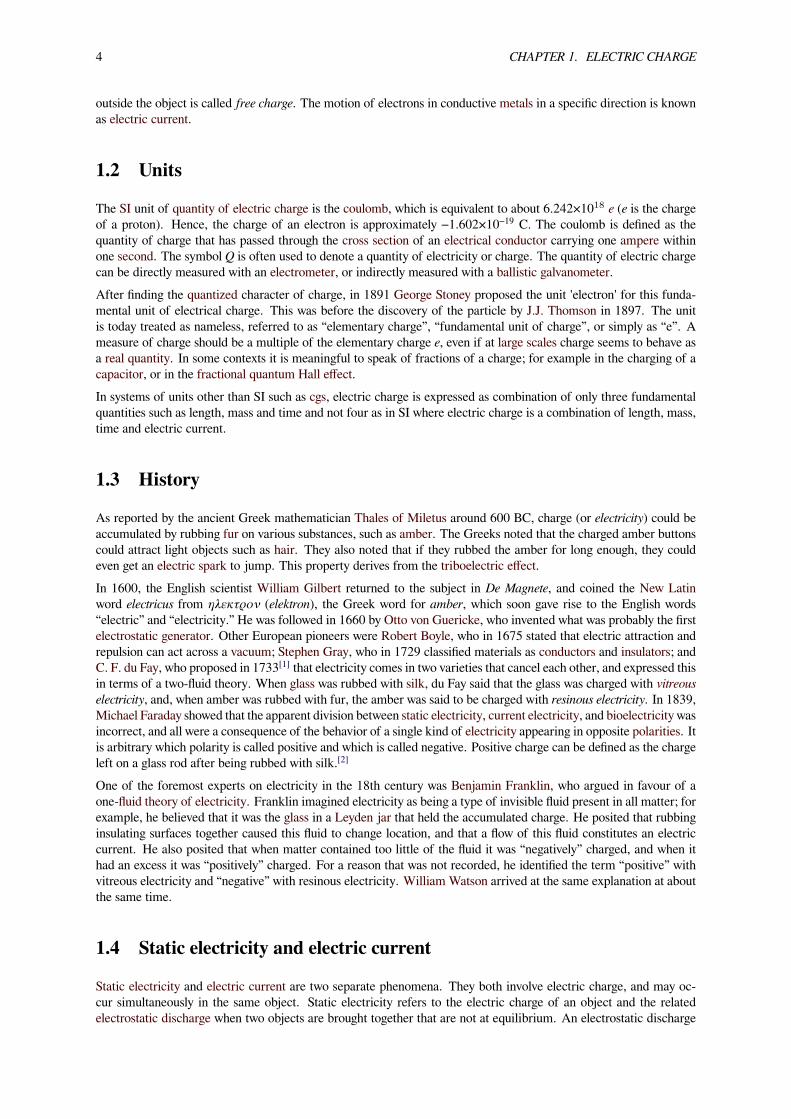
Electric charge is the physical property of matter that causes it to experience a force when placed in an electro-magnetic field. There are two types of electric charges: positive and negative. Positively charged substances arerepelled from other positively charged substances, but attracted to negatively charged substances; negatively chargedsubstances are repelled from negative and attracted to positive. An object is negatively charged if it has an excessof electrons, and is otherwise positively charged or uncharged. The SI derived unit of electric charge is the coulomb(C), although in electrical engineering it is also common to use the ampere-hour (Ah), and in chemistry it is commonto use the elementary charge (e) as a unit. The symbol Q is often used to denote charge. The early knowledge of howcharged substances interact is now called classical electrodynamics, and is still very accurate if quantum effects donot need to be considered.The electric charge is a fundamental conserved property of some subatomic particles, which determines their electromagneticinteraction. Electrically charged matter is influenced by, and produces, electromagnetic fields. The interaction be-

1

2 CHAPTER 1. ELECTRIC CHARGE

tween a moving charge and an electromagnetic field is the source of the electromagnetic force, which is one of thefour fundamental forces (See also: magnetic field).Twentieth-century experiments demonstrated that electric charge is quantized; that is, it comes in integer multiplesof individual small units called the elementary charge, e, approximately equal to 1.602×10−19 coulombs (except forparticles called quarks, which have charges that are integer multiples of e/3). The proton has a charge of +e, and theelectron has a charge of −e. The study of charged particles, and how their interactions are mediated by photons, iscalled quantum electrodynamics.

1.1 Overview

Diagram showing field lines and equipotentials around an electron, a negatively charged particle. In an electrically neutral atom,the number of electrons is equal to the number of protons (which are positively charged), resulting in a net zero overall charge

Charge is the fundamental property of forms of matter that exhibit electrostatic attraction or repulsion in the presenceof other matter. Electric charge is a characteristic property of many subatomic particles. The charges of free-standingparticles are integer multiples of the elementary charge e; we say that electric charge is quantized. Michael Faraday,in his electrolysis experiments, was the first to note the discrete nature of electric charge. Robert Millikan's oil-dropexperiment demonstrated this fact directly, and measured the elementary charge.By convention, the charge of an electron is −1, while that of a proton is +1. Charged particles whose charges have

1.1. OVERVIEW 3

the same sign repel one another, and particles whose charges have different signs attract. Coulomb’s law quantifiesthe electrostatic force between two particles by asserting that the force is proportional to the product of their charges,and inversely proportional to the square of the distance between them.The charge of an antiparticle equals that of the corresponding particle, but with opposite sign. Quarks have fractionalcharges of either −1⁄3 or +2⁄3, but free-standing quarks have never been observed (the theoretical reason for this factis asymptotic freedom).The electric charge of a macroscopic object is the sum of the electric charges of the particles that make it up. Thischarge is often small, because matter is made of atoms, and atoms typically have equal numbers of protons andelectrons, in which case their charges cancel out, yielding a net charge of zero, thus making the atom neutral.An ion is an atom (or group of atoms) that has lost one or more electrons, giving it a net positive charge (cation),or that has gained one or more electrons, giving it a net negative charge (anion). Monatomic ions are formed fromsingle atoms, while polyatomic ions are formed from two or more atoms that have been bonded together, in each caseyielding an ion with a positive or negative net charge.

Electric field induced by a positive electric charge (left) and a field induced by a negative electric charge (right).

During formation of macroscopic objects, constituent atoms and ions usually combine to form structures composedof neutral ionic compounds electrically bound to neutral atoms. Thus macroscopic objects tend toward being neutraloverall, but macroscopic objects are rarely perfectly net neutral.Sometimes macroscopic objects contain ions distributed throughout the material, rigidly bound in place, giving anoverall net positive or negative charge to the object. Also, macroscopic objects made of conductive elements, canmore or less easily (depending on the element) take on or give off electrons, and then maintain a net negative orpositive charge indefinitely. When the net electric charge of an object is non-zero and motionless, the phenomenon isknown as static electricity. This can easily be produced by rubbing two dissimilar materials together, such as rubbingamber with fur or glass with silk. In this way non-conductive materials can be charged to a significant degree, eitherpositively or negatively. Charge taken from one material is moved to the other material, leaving an opposite chargeof the same magnitude behind. The law of conservation of charge always applies, giving the object from which anegative charge has been taken a positive charge of the same magnitude, and vice versa.Even when an object’s net charge is zero, charge can be distributed non-uniformly in the object (e.g., due to anexternal electromagnetic field, or bound polar molecules). In such cases the object is said to be polarized. The chargedue to polarization is known as bound charge, while charge on an object produced by electrons gained or lost from

4 CHAPTER 1. ELECTRIC CHARGE

outside the object is called free charge. The motion of electrons in conductive metals in a specific direction is knownas electric current.

1.2 Units

The SI unit of quantity of electric charge is the coulomb, which is equivalent to about 6.242×1018 e (e is the chargeof a proton). Hence, the charge of an electron is approximately −1.602×10−19 C. The coulomb is defined as thequantity of charge that has passed through the cross section of an electrical conductor carrying one ampere withinone second. The symbol Q is often used to denote a quantity of electricity or charge. The quantity of electric chargecan be directly measured with an electrometer, or indirectly measured with a ballistic galvanometer.After finding the quantized character of charge, in 1891 George Stoney proposed the unit 'electron' for this funda-mental unit of electrical charge. This was before the discovery of the particle by J.J. Thomson in 1897. The unitis today treated as nameless, referred to as “elementary charge”, “fundamental unit of charge”, or simply as “e”. Ameasure of charge should be a multiple of the elementary charge e, even if at large scales charge seems to behave asa real quantity. In some contexts it is meaningful to speak of fractions of a charge; for example in the charging of acapacitor, or in the fractional quantum Hall effect.In systems of units other than SI such as cgs, electric charge is expressed as combination of only three fundamentalquantities such as length, mass and time and not four as in SI where electric charge is a combination of length, mass,time and electric current.

1.3 History

As reported by the ancient Greek mathematician Thales of Miletus around 600 BC, charge (or electricity) could beaccumulated by rubbing fur on various substances, such as amber. The Greeks noted that the charged amber buttonscould attract light objects such as hair. They also noted that if they rubbed the amber for long enough, they couldeven get an electric spark to jump. This property derives from the triboelectric effect.In 1600, the English scientist William Gilbert returned to the subject in De Magnete, and coined the New Latinword electricus from ηλεκτρον (elektron), the Greek word for amber, which soon gave rise to the English words“electric” and “electricity.” He was followed in 1660 by Otto von Guericke, who invented what was probably the firstelectrostatic generator. Other European pioneers were Robert Boyle, who in 1675 stated that electric attraction andrepulsion can act across a vacuum; Stephen Gray, who in 1729 classified materials as conductors and insulators; andC. F. du Fay, who proposed in 1733[1] that electricity comes in two varieties that cancel each other, and expressed thisin terms of a two-fluid theory. When glass was rubbed with silk, du Fay said that the glass was charged with vitreouselectricity, and, when amber was rubbed with fur, the amber was said to be charged with resinous electricity. In 1839,Michael Faraday showed that the apparent division between static electricity, current electricity, and bioelectricity wasincorrect, and all were a consequence of the behavior of a single kind of electricity appearing in opposite polarities. Itis arbitrary which polarity is called positive and which is called negative. Positive charge can be defined as the chargeleft on a glass rod after being rubbed with silk.[2]

One of the foremost experts on electricity in the 18th century was Benjamin Franklin, who argued in favour of aone-fluid theory of electricity. Franklin imagined electricity as being a type of invisible fluid present in all matter; forexample, he believed that it was the glass in a Leyden jar that held the accumulated charge. He posited that rubbinginsulating surfaces together caused this fluid to change location, and that a flow of this fluid constitutes an electriccurrent. He also posited that when matter contained too little of the fluid it was “negatively” charged, and when ithad an excess it was “positively” charged. For a reason that was not recorded, he identified the term “positive” withvitreous electricity and “negative” with resinous electricity. William Watson arrived at the same explanation at aboutthe same time.

1.4 Static electricity and electric current

Static electricity and electric current are two separate phenomena. They both involve electric charge, and may oc-cur simultaneously in the same object. Static electricity refers to the electric charge of an object and the relatedelectrostatic discharge when two objects are brought together that are not at equilibrium. An electrostatic discharge

1.4. STATIC ELECTRICITY AND ELECTRIC CURRENT 5

Coulomb’s torsion balance

creates a change in the charge of each of the two objects. In contrast, electric current is the flow of electric chargethrough an object, which produces no net loss or gain of electric charge.

1.4.1 Electrification by friction

Further information: triboelectric effect

6 CHAPTER 1. ELECTRIC CHARGE

When a piece of glass and a piece of resin—neither of which exhibit any electrical properties—are rubbed togetherand left with the rubbed surfaces in contact, they still exhibit no electrical properties. When separated, they attracteach other.A second piece of glass rubbed with a second piece of resin, then separated and suspended near the former pieces ofglass and resin causes these phenomena:

• The two pieces of glass repel each other.

• Each piece of glass attracts each piece of resin.

• The two pieces of resin repel each other.

This attraction and repulsion is an electrical phenomena, and the bodies that exhibit them are said to be electrified, orelectrically charged. Bodies may be electrified in many other ways, as well as by friction. The electrical properties ofthe two pieces of glass are similar to each other but opposite to those of the two pieces of resin: The glass attractswhat the resin repels and repels what the resin attracts.If a body electrified in any manner whatsoever behaves as the glass does, that is, if it repels the glass and attractsthe resin, the body is said to be 'vitreously' electrified, and if it attracts the glass and repels the resin it is said to be'resinously' electrified. All electrified bodies are found to be either vitreously or resinously electrified.It is the established convention of the scientific community to define the vitreous electrification as positive, and theresinous electrification as negative. The exactly opposite properties of the two kinds of electrification justify ourindicating them by opposite signs, but the application of the positive sign to one rather than to the other kind must beconsidered as a matter of arbitrary convention, just as it is a matter of convention in mathematical diagram to reckonpositive distances towards the right hand.No force, either of attraction or of repulsion, can be observed between an electrified body and a body not electrified.[3]

Actually, all bodies are electrified, but may appear not to be so by the relative similar charge of neighboring objects inthe environment. An object further electrified + or – creates an equivalent or opposite charge by default in neighboringobjects, until those charges can equalize. The effects of attraction can be observed in high-voltage experiments, whilelower voltage effects are merely weaker and therefore less obvious. The attraction and repulsion forces are codified byCoulomb’s Law (attraction falls off at the square of the distance, which has a corollary for acceleration in a gravitationalfield, suggesting that gravitation may be merely electrostatic phenomenon between relatively weak charges in termsof scale). See also the Casimir effect.It is now known that the Franklin/Watson model was fundamentally correct. There is only one kind of electricalcharge, and only one variable is required to keep track of the amount of charge.[4] On the other hand, just knowingthe charge is not a complete description of the situation. Matter is composed of several kinds of electrically chargedparticles, and these particles have many properties, not just charge.The most common charge carriers are the positively charged proton and the negatively charged electron. The move-ment of any of these charged particles constitutes an electric current. In many situations, it suffices to speak ofthe conventional current without regard to whether it is carried by positive charges moving in the direction of theconventional current or by negative charges moving in the opposite direction. This macroscopic viewpoint is anapproximation that simplifies electromagnetic concepts and calculations.At the opposite extreme, if one looks at the microscopic situation, one sees there are many ways of carrying an electriccurrent, including: a flow of electrons; a flow of electron "holes" that act like positive particles; and both negativeand positive particles (ions or other charged particles) flowing in opposite directions in an electrolytic solution or aplasma.Beware that, in the common and important case of metallic wires, the direction of the conventional current is oppositeto the drift velocity of the actual charge carriers, i.e., the electrons. This is a source of confusion for beginners.

1.5 Properties

Aside from the properties described in articles about electromagnetism, charge is a relativistic invariant. This meansthat any particle that has charge Q, no matter how fast it goes, always has charge Q. This property has been experi-mentally verified by showing that the charge of one helium nucleus (two protons and two neutrons bound together in

1.6. CONSERVATION OF ELECTRIC CHARGE 7

a nucleus and moving around at high speeds) is the same as two deuterium nuclei (one proton and one neutron boundtogether, but moving much more slowly than they would if they were in a helium nucleus).

1.6 Conservation of electric charge

Main article: Charge conservation

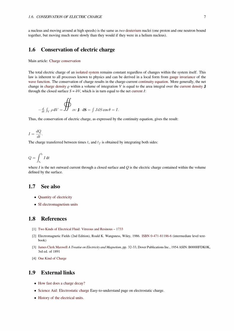
The total electric charge of an isolated system remains constant regardless of changes within the system itself. Thislaw is inherent to all processes known to physics and can be derived in a local form from gauge invariance of thewave function. The conservation of charge results in the charge-current continuity equation. More generally, the netchange in charge density ρ within a volume of integration V is equal to the area integral over the current density Jthrough the closed surface S = ∂V, which is in turn equal to the net current I:

− ddt

∫Vρ dV = ∂V J · dS =

∫JdS cos θ = I.

Thus, the conservation of electric charge, as expressed by the continuity equation, gives the result:

I =dQ

dt.

The charge transferred between times ti and tf is obtained by integrating both sides:

Q =

∫ tf

ti

I dt

where I is the net outward current through a closed surface and Q is the electric charge contained within the volumedefined by the surface.

1.7 See also• Quantity of electricity• SI electromagnetism units

1.8 References[1] Two Kinds of Electrical Fluid: Vitreous and Resinous – 1733

[2] Electromagnetic Fields (2nd Edition), Roald K. Wangsness, Wiley, 1986. ISBN 0-471-81186-6 (intermediate level text-book)

[3] JamesClerkMaxwellATreatise on Electricity andMagnetism, pp. 32-33, Dover Publications Inc., 1954ASIN: B000HFDK0K,3rd ed. of 1891

[4] One Kind of Charge

1.9 External links• How fast does a charge decay?• Science Aid: Electrostatic charge Easy-to-understand page on electrostatic charge.• History of the electrical units.

Chapter 2

Electrostatic induction

Electrostatic induction is a redistribution of electrical charge in an object, caused by the influence of nearbycharges.[1] In the presence of a charged body, an insulated conductor develops a positive charge on one end anda negative charge on the other end.[1] Induction was discovered by British scientist John Canton in 1753 and Swedishprofessor Johan Carl Wilcke in 1762.[2] Electrostatic generators, such as the Wimshurst machine, the Van de Graaffgenerator and the electrophorus, use this principle. Due to induction, the electrostatic potential (voltage) is constantat any point throughout a conductor.[3] Induction is also responsible for the attraction of light nonconductive objects,such as balloons, paper or styrofoam scraps, to static electric charges. Electrostatic induction should not be confusedwith electromagnetic induction.

2.1 Explanation

Demonstration of induction, in the 1870s. The positive terminal of an electrostatic machine is placed near an uncharged brasscylinder, causing the left end to acquire a positive charge and the right to acquire a negative charge. The small pith ball electroscopeshanging from the bottom show that the charge is concentrated at the ends.

8

2.2. CHARGING AN OBJECT BY INDUCTION 9

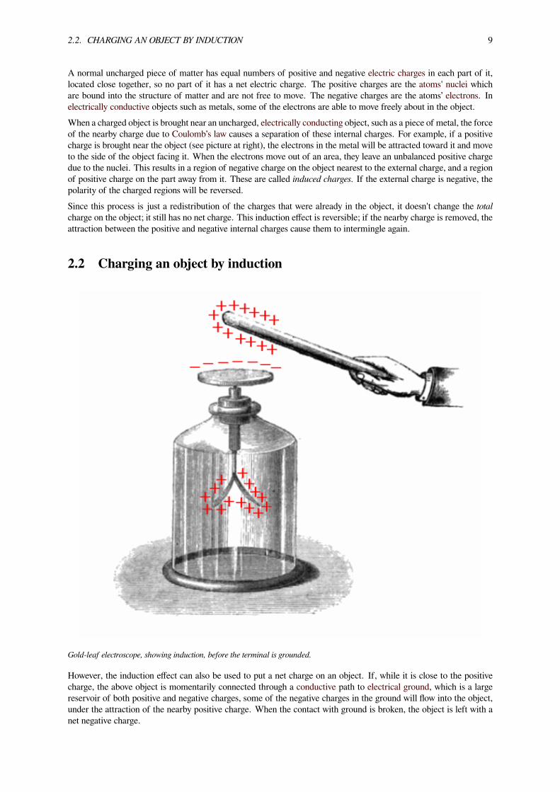
A normal uncharged piece of matter has equal numbers of positive and negative electric charges in each part of it,located close together, so no part of it has a net electric charge. The positive charges are the atoms' nuclei whichare bound into the structure of matter and are not free to move. The negative charges are the atoms’ electrons. Inelectrically conductive objects such as metals, some of the electrons are able to move freely about in the object.When a charged object is brought near an uncharged, electrically conducting object, such as a piece of metal, the forceof the nearby charge due to Coulomb’s law causes a separation of these internal charges. For example, if a positivecharge is brought near the object (see picture at right), the electrons in the metal will be attracted toward it and moveto the side of the object facing it. When the electrons move out of an area, they leave an unbalanced positive chargedue to the nuclei. This results in a region of negative charge on the object nearest to the external charge, and a regionof positive charge on the part away from it. These are called induced charges. If the external charge is negative, thepolarity of the charged regions will be reversed.Since this process is just a redistribution of the charges that were already in the object, it doesn't change the totalcharge on the object; it still has no net charge. This induction effect is reversible; if the nearby charge is removed, theattraction between the positive and negative internal charges cause them to intermingle again.

2.2 Charging an object by induction

Gold-leaf electroscope, showing induction, before the terminal is grounded.

However, the induction effect can also be used to put a net charge on an object. If, while it is close to the positivecharge, the above object is momentarily connected through a conductive path to electrical ground, which is a largereservoir of both positive and negative charges, some of the negative charges in the ground will flow into the object,under the attraction of the nearby positive charge. When the contact with ground is broken, the object is left with anet negative charge.

10 CHAPTER 2. ELECTROSTATIC INDUCTION

This method can be demonstrated using a gold-leaf electroscope, which is an instrument for detecting electric charge.The electroscope is first discharged, and a charged object is then brought close to the instrument’s top terminal.Induction causes a separation of the charges inside the electroscope's metal rod, so that the top terminal gains a netcharge of opposite polarity to that of the object, while the gold leaves gain a charge of the same polarity. Sinceboth leaves have the same charge, they repel each other and spread apart. The electroscope has not acquired a netcharge: the charge within it has merely been redistributed, so if the charged object were to be moved away from theelectroscope the leaves will come together again.But if an electrical contact is now brieflymade between the electroscope terminal and ground, for example by touchingthe terminal with a finger, this causes charge to flow from ground to the terminal, attracted by the charge on the objectclose to the terminal. This charge neutralizes the charge in the gold leaves, so the leaves come together again. Theelectroscope now contains a net charge opposite in polarity to that of the charged object. When the electrical contactto earth is broken, e.g. by lifting the finger, the extra charge that has just flowed into the electroscope cannot escape,and the instrument retains a net charge. The charge is held in the top of the electroscope terminal by the attractionof the inducing charge. But when the inducing charge is moved away, the charge is released and spreads throughoutthe electroscope terminal to the leaves, so the gold leaves move apart again.The sign of the charge left on the electroscope after grounding is always opposite in sign to the external inducingcharge.[4] The two rules of induction are:[4][5]

• If the object is not grounded, the nearby charge will induce equal and opposite charges in the object.

• If any part of the object is momentarily grounded while the inducing charge is near, a charge opposite inpolarity to the inducing charge will be attracted from ground into the object, and it will be left with a chargeopposite to the inducing charge.

2.3 The electrostatic field inside a conductive object is zero

A remaining question is how large the induced charges are. The movement of charge is caused by the force exertedby the electric field of the external charged object, by Coulomb’s law. As the charges in the metal object continueto separate, the resulting positive and negative regions create their own electric field, which opposes the field of theexternal charge.[3] This process continues until very quickly (within a fraction of a second) an equilibrium is reachedin which the induced charges are exactly the right size to cancel the external electric field throughout the interior ofthe metal object.[3][6] Then the remaining mobile charges (electrons) in the interior of the metal no longer feel a forceand the net motion of the charges stops.[3]

2.4 Induced charge resides on the surface

Since the mobile charges in the interior of a metal object are free to move in any direction, there can never be astatic concentration of charge inside the metal; if there was, it would attract opposite polarity charge to neutralizeit.[3] Therefore in induction, the mobile charges move under the influence of the external charge until they reach thesurface of the metal and collect there, where they are constrained from moving by the boundary.[3]

This establishes the important principle that electrostatic charges on conductive objects reside on the surface of theobject.[3][6] External electric fields induce surface charges on metal objects that exactly cancel the field within.[3] Sincethe field is the gradient of the electrostatic potential, another way of saying this is that in electrostatics, the potential(voltage) throughout a conductive object is constant.[3]

2.5 Induction in dielectric objects

A similar induction effect occurs in nonconductive (dielectric) objects, and is responsible for the attraction of smalllight nonconductive objects, like balloons, scraps of paper or Styrofoam, to static electric charges.[7][8][9][10] In non-conductors, the electrons are bound to atoms or molecules and are not free to move about the object as in conductors;however they can move a little within the molecules.If a positive charge is brought near a nonconductive object, the electrons in each molecule are attracted toward it,and move to the side of the molecule facing the charge, while the positive nuclei are repelled and move slightly to

2.5. INDUCTION IN DIELECTRIC OBJECTS 11

−

− − −−−−−−++

+ + + + + +

−−−−

+

+

+

++

− −−−− − − −

+ + + + +++

+

Surface charges induced in metal objects by a nearby charge. The electrostatic field (lines with arrows) of a nearby positive charge(+) causes the mobile charges in metal objects to separate. Negative charges (blue) are attracted and move to the surface of the objectfacing the external charge. Positive charges (red) are repelled and move to the surface facing away. These induced surface chargescreate an opposing electric field that exactly cancels the field of the external charge throughout the interior of the metal. Thereforeelectrostatic induction ensures that the electric field everywhere inside a conductive object is zero.

the opposite side of the molecule. Since the negative charges are now closer to the external charge than the positive

12 CHAPTER 2. ELECTROSTATIC INDUCTION

charges, their attraction is greater than the repulsion of the positive charges, resulting in a small net attraction of themolecule toward the charge. This is called polarization, and the polarized molecules are called dipoles. This effect ismicroscopic, but since there are so many molecules, it adds up to enough force to move a light object like Styrofoam.This is the principle of operation of a pith-ball electroscope.[11]

2.6 Notes[1] “Electrostatic induction”. Encyclopaedia Britannica Online. Encyclopaedia Britannica, Inc. 2008. Retrieved 2008-06-25.

[2] “Electricity”. Encyclopaedia Britannica, 11th Ed. 9. The Encyclopaedia Britannica Co. 1910. p. 181. Retrieved 2008-06-23.

[3] Purcell, Edward M.; David J. Morin (2013). Electricity and Magnetism. Cambridge Univ. Press. pp. 127–128. ISBN1107014026.

[4] Cope, Thomas A. Darlington. Physics. Library of Alexandria. ISBN 1465543724.

[5] Hadley, Harry Edwin (1899). Magnetism & Electricity for Beginners. Macmillan & Company. p. 182.

[6] Saslow, Wayne M. (2002). Electricity, magnetism, and light. US: Academic Press. pp. 159–161. ISBN 0-12-619455-6.

[7] Sherwood, Bruce A.; Ruth W. Chabay (2011). Matter and Interactions, 3rd Ed. USA: John Wiley and Sons. pp. 594–596.ISBN 0-470-50347-5.

[8] Paul E. Tippens, Electric Charge and Electric Force, Powerpoint presentation, p.27-28, 2009, S. Polytechnic State Univ. onDocStoc.com website

[9] Henderson, Tom (2011). “Charge and Charge Interactions”. Static Electricity, Lesson 1. The Physics Classroom. Retrieved2012-01-01.

[10] Winn, Will (2010). Introduction to Understandable Physics Vol. 3: Electricity, Magnetism and Ligh. USA: Author House.p. 20.4. ISBN 1-4520-1590-2.

[11] Kaplan MCAT Physics 2010-2011. USA: Kaplan Publishing. 2009. p. 329. ISBN 1-4277-9875-3.

2.7 External links• “Charging by electrostatic induction”. Regents exam prep center. Oswego City School District. 1999. Retrieved2008-06-25.

Chapter 3

Coulomb’s law

Coulomb’s law, orCoulomb’s inverse-square law, is a law of physics describing the electrostatic interaction betweenelectrically charged particles. The law was first published in 1784 by French physicist Charles Augustin de Coulomband was essential to the development of the theory of electromagnetism. It is analogous to Isaac Newton's inverse-square law of universal gravitation. Coulomb’s law can be used to derive Gauss’s law, and vice versa. The law hasbeen tested heavily, and all observations have upheld the law’s principle.

3.1 History

Ancient cultures around the Mediterranean knew that certain objects, such as rods of amber, could be rubbed withcat’s fur to attract light objects like feathers. Thales ofMiletusmade a series of observations on static electricity around600 BC, from which he believed that friction rendered amber magnetic, in contrast to minerals such as magnetite,which needed no rubbing.[1][2] Thales was incorrect in believing the attraction was due to a magnetic effect, but laterscience would prove a link betweenmagnetism and electricity. Electricity would remain little more than an intellectualcuriosity for millennia until 1600, when the English scientist William Gilbert made a careful study of electricity andmagnetism, distinguishing the lodestone effect from static electricity produced by rubbing amber.[1] He coined theNew Latin word electricus (“of amber” or “like amber”, from ήλεκτρον [elektron], the Greek word for “amber”) torefer to the property of attracting small objects after being rubbed.[3] This association gave rise to the English words“electric” and “electricity”, which made their first appearance in print in Thomas Browne's Pseudodoxia Epidemicaof 1646.[4]

Early investigators of the 18th century who suspected that the electrical force diminished with distance as the forceof gravity did (i.e., as the inverse square of the distance) included Daniel Bernoulli[5] and Alessandro Volta, both ofwhom measured the force between plates of a capacitor, and Franz Aepinus who supposed the inverse-square law in1758.[6]

Based on experiments with electrically charged spheres, Joseph Priestley of England was among the first to proposethat electrical force followed an inverse-square law, similar to Newton’s law of universal gravitation. However, hedid not generalize or elaborate on this.[7] In 1767, he conjectured that the force between charges varied as the inversesquare of the distance.[8][9]

In 1769, Scottish physicist John Robison announced that, according to his measurements, the force of repulsionbetween two spheres with charges of the same sign varied as x−2.06.[10]

In the early 1770s, the dependence of the force between charged bodies upon both distance and charge had alreadybeen discovered, but not published, by Henry Cavendish of England.[11]

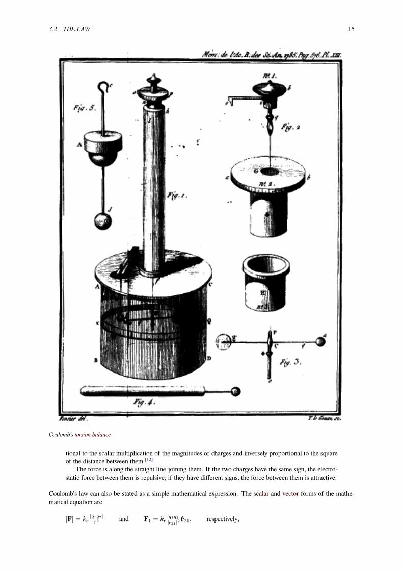
Finally, in 1785, the French physicist Charles-Augustin de Coulomb published his first three reports of electricityand magnetism where he stated his law. This publication was essential to the development of the theory of elec-tromagnetism.[12] He used a torsion balance to study the repulsion and attraction forces of charged particles, anddetermined that the magnitude of the electric force between two point charges is directly proportional to the productof the charges and inversely proportional to the square of the distance between them.The torsion balance consists of a bar suspended from its middle by a thin fiber. The fiber acts as a very weak torsionspring. In Coulomb’s experiment, the torsion balance was an insulating rod with a metal-coated ball attached to one

13

14 CHAPTER 3. COULOMB’S LAW

Charles-Augustin de Coulomb

end, suspended by a silk thread. The ball was charged with a known charge of static electricity, and a second chargedball of the same polarity was brought near it. The two charged balls repelled one another, twisting the fiber througha certain angle, which could be read from a scale on the instrument. By knowing how much force it took to twist thefiber through a given angle, Coulomb was able to calculate the force between the balls and derive his inverse-squareproportionality law.

3.2 The law

Coulomb’s law states that:

The magnitude of the electrostatic force of interaction between two point charges is directly propor-

3.2. THE LAW 15

Coulomb’s torsion balance

tional to the scalar multiplication of the magnitudes of charges and inversely proportional to the squareof the distance between them.[12]

The force is along the straight line joining them. If the two charges have the same sign, the electro-static force between them is repulsive; if they have different signs, the force between them is attractive.

Coulomb’s law can also be stated as a simple mathematical expression. The scalar and vector forms of the mathe-matical equation are

|F| = ke|q1q2|r2 and F1 = ke

q1q2|r21|2 r̂21, respectively,

16 CHAPTER 3. COULOMB’S LAW

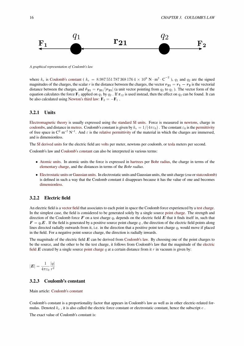
A graphical representation of Coulomb’s law

where ke is Coulomb’s constant ( ke = 8.987 551 787 368 176 4 × 109 N ·m2 · C−2 ), q1 and q2 are the signedmagnitudes of the charges, the scalar r is the distance between the charges, the vector r21 = r1 − r2 is the vectorialdistance between the charges, and r̂21 = r21/|r21| (a unit vector pointing from q2 to q1 ). The vector form of theequation calculates the force F1 applied on q1 by q2 . If r12 is used instead, then the effect on q2 can be found. It canbe also calculated using Newton’s third law: F2 = −F1 .

3.2.1 Units

Electromagnetic theory is usually expressed using the standard SI units. Force is measured in newtons, charge incoulombs, and distance in metres. Coulomb’s constant is given by ke = 1/(4πε0) . The constant ε0 is the permittivityof free space in C2 m−2 N−1. And ε is the relative permittivity of the material in which the charges are immersed,and is dimensionless.The SI derived units for the electric field are volts per meter, newtons per coulomb, or tesla meters per second.Coulomb’s law and Coulomb’s constant can also be interpreted in various terms:

• Atomic units. In atomic units the force is expressed in hartrees per Bohr radius, the charge in terms of theelementary charge, and the distances in terms of the Bohr radius.

• Electrostatic units or Gaussian units. In electrostatic units andGaussian units, the unit charge (esu or statcoulomb)is defined in such a way that the Coulomb constant k disappears because it has the value of one and becomesdimensionless.

3.2.2 Electric field

An electric field is a vector field that associates to each point in space the Coulomb force experienced by a test charge.In the simplest case, the field is considered to be generated solely by a single source point charge. The strength anddirection of the Coulomb force F on a test charge qt depends on the electric field E that it finds itself in, such thatF = qtE . If the field is generated by a positive source point charge q , the direction of the electric field points alonglines directed radially outwards from it, i.e. in the direction that a positive point test charge qt would move if placedin the field. For a negative point source charge, the direction is radially inwards.The magnitude of the electric field E can be derived from Coulomb’s law. By choosing one of the point charges tobe the source, and the other to be the test charge, it follows from Coulomb’s law that the magnitude of the electricfield E created by a single source point charge q at a certain distance from it r in vacuum is given by:

|E| = 1

4πε0

|q|r2

3.2.3 Coulomb’s constant

Main article: Coulomb’s constant

Coulomb’s constant is a proportionality factor that appears in Coulomb’s law as well as in other electric-related for-mulas. Denoted ke , it is also called the electric force constant or electrostatic constant, hence the subscript e .The exact value of Coulomb’s constant is:

3.3. SCALAR FORM 17

If the two charges have the same sign, the electrostatic force between them is repulsive; if they have different sign, the force betweenthem is attractive.

ke =1

4πε0=

c20µ0

4π= c20 × 10−7 H ·m−1

= 8.987 551 787 368 176 4× 109 N ·m2 · C−2

3.2.4 Conditions for validity

There are three conditions to be fulfilled for the validity of Coulomb’s law:

1. The charges considered must be point charges.

2. They should be stationary with respect to each other.

3. The two point charges should be placed in a single medium.

18 CHAPTER 3. COULOMB’S LAW

F Fq Q

r

+

IF I IF IQ-q q-Q= = _kIq QI×

r 2

Fq+

FQ+

Q-q

Q-q

q-Q

q-Q

The absolute value of the force F between two point charges q and Q relates to the distance between the point charges and to thesimple product of their charges. The diagram shows that like charges repel each other, and opposite charges attract each other.

3.3 Scalar form

When it is only of interest to know the magnitude of the electrostatic force (and not its direction), it may be easiestto consider a scalar version of the law. The scalar form of Coulomb’s Law relates the magnitude and sign of theelectrostatic force F acting simultaneously on two point charges q1 and q2 as follows:

|F | = ke|q1q2|r2

where r is the separation distance and ke is Coulomb’s constant. If the product q1q2 is positive, the force betweenthe two charges is repulsive; if the product is negative, the force between them is attractive.[13]

3.4 Vector form

Coulomb’s law states that the electrostatic force F1 experienced by a charge, q1 at position r1 , in the vicinity ofanother charge, q2 at position r2 , in a vacuum is equal to:

F1 =q1q24πε0

(r1 − r2)

|r1 − r2|3=

q1q24πε0

r̂21|r21|2

,

where r21 = r1 − r2 , the unit vector r̂21 = r21/|r21| , and ε0 is the electric constant.The vector form of Coulomb’s law is simply the scalar definition of the law with the direction given by the unit vector,r̂21 , parallel with the line from charge q2 to charge q1 .[14] If both charges have the same sign (like charges) then

3.4. VECTOR FORM 19

In the image, the vector F 1 is the force experienced by q1 , and the vector F 2 is the force experienced by q2 . When q1q2 > 0 theforces are repulsive (as in the image) and when q1q2 < 0 the forces are attractive (opposite to the image). The magnitude of theforces will always be equal.

the product q1q2 is positive and the direction of the force on q1 is given by r̂21 ; the charges repel each other. If thecharges have opposite signs then the product q1q2 is negative and the direction of the force on q1 is given by −r̂21 ;the charges attract each other.The electrostatic force F2 experienced by q2 , according to Newton’s third law, is F2 = −F1 .

3.4.1 System of discrete charges

The law of superposition allows Coulomb’s law to be extended to include any number of point charges. The forceacting on a point charge due to a system of point charges is simply the vector addition of the individual forces actingalone on that point charge due to each one of the charges. The resulting force vector is parallel to the electric fieldvector at that point, with that point charge removed.The force F on a small charge, q at position r , due to a system of N discrete charges in vacuum is:

F (r) =q

4πε0

N∑i=1

qir − ri

|r − ri|3=

q

4πε0

N∑i=1

qiR̂i

|Ri|2,

where qi and ri are the magnitude and position respectively of the ith charge, R̂i is a unit vector in the direction ofRi = r − ri (a vector pointing from charges qi to q ).[14]

3.4.2 Continuous charge distribution

In this case, the principle of linear superposition is also used. For a continuous charge distribution, an integral overthe region containing the charge is equivalent to an infinite summation, treating each infinitesimal element of spaceas a point charge dq . The distribution of charge is usually linear, surface or volumetric.For a linear charge distribution (a good approximation for charge in a wire) where λ(r′) gives the charge per unitlength at position r′ , and dl′ is an infinitesimal element of length,

dq = λ(r′)dl′ .[15]

For a surface charge distribution (a good approximation for charge on a plate in a parallel plate capacitor) whereσ(r′) gives the charge per unit area at position r′ , and dA′ is an infinitesimal element of area,

dq = σ(r′) dA′.

For a volume charge distribution (such as charge within a bulk metal) where ρ(r′) gives the charge per unit volumeat position r′ , and dV ′ is an infinitesimal element of volume,

dq = ρ(r′) dV ′. [14]

The force on a small test charge q′ at position r in vacuum is given by the integral over the distribution of charge:

F =q′

4πε0

∫dq

r − r′

|r − r′|3.

20 CHAPTER 3. COULOMB’S LAW

3.5 Simple experiment to verify Coulomb’s law

Experiment to verify Coulomb’s law.

It is possible to verify Coulomb’s law with a simple experiment. Let’s consider two small spheres of mass m andsame-sign charge q , hanging from two ropes of negligible mass of length l . The forces acting on each sphere arethree: the weightmg , the rope tension T and the electric force F .In the equilibrium state:and:Dividing (1) by (2):Being L1 the distance between the charged spheres; the repulsion force between them F1 , assuming Coulomb’s lawis correct, is equal toso:If we now discharge one of the spheres, and we put it in contact with the charged sphere, each one of them acquiresa charge q/2. In the equilibrium state, the distance between the charges will be L2 < L1 and the repulsion forcebetween them will be:We know that F2 = mg. tan θ2 . And:

q2

4

4πϵ0L22

= mg. tan θ2

Dividing (4) by (5), we get:Measuring the angles θ1 and θ2 and the distance between the charges L1 and L2 is sufficient to verify that the equalityis true taking into account the experimental error. In practice, angles can be difficult to measure, so if the length ofthe ropes is sufficiently great, the angles will be small enough to make the following approximation:

3.6. ELECTROSTATIC APPROXIMATION 21

Using this approximation, the relationship (6) becomes the much simpler expression:In this way, the verification is limited to measuring the distance between the charges and check that the divisionapproximates the theoretical value.

3.6 Electrostatic approximation

In either formulation, Coulomb’s law is fully accurate only when the objects are stationary, and remains approximatelycorrect only for slow movement. These conditions are collectively known as the electrostatic approximation. Whenmovement takes place, magnetic fields that alter the force on the two objects are produced. The magnetic interactionbetween moving charges may be thought of as a manifestation of the force from the electrostatic field but withEinstein’s theory of relativity taken into consideration.

3.6.1 Atomic forces

Coulomb’s law holds even within atoms, correctly describing the force between the positively charged atomic nucleusand each of the negatively charged electrons. This simple law also correctly accounts for the forces that bind atomstogether to form molecules and for the forces that bind atoms and molecules together to form solids and liquids.Generally, as the distance between ions increases, the energy of attraction approaches zero and ionic bonding is lessfavorable. As the magnitude of opposing charges increases, energy increases and ionic bonding is more favorable.

3.7 See also• Biot–Savart law

• Gauss’s law

• Method of image charges

• Electromagnetic force

• Molecular modelling

• Static forces and virtual-particle exchange

• Darwin Lagrangian

• Newton’s law of universal gravitation, which uses a similar structure, but for mass instead of charge.

3.8 Notes[1] Stewart, Joseph (2001). Intermediate Electromagnetic Theory. World Scientific. p. 50. ISBN 981-02-4471-1

[2] Simpson, Brian (2003). Electrical Stimulation and the Relief of Pain. Elsevier Health Sciences. pp. 6–7. ISBN 0-444-51258-6

[3] Baigrie, Brian (2006). Electricity and Magnetism: A Historical Perspective. Greenwood Press. pp. 7–8. ISBN 0-313-33358-0

[4] Chalmers, Gordon (1937). “The Lodestone and the Understanding of Matter in Seventeenth Century England”. Philosophyof Science 4 (1): 75–95. doi:10.1086/286445

[5] Socin, Abel (1760). Acta Helvetica Physico-Mathematico-Anatomico-Botanico-Medica (in Latin) 4. Basileae. pp. 224,225.

[6] Heilbron, J.L. (1979). Electricity in the 17th and 18th Centuries: A Study of Early Modern Physics. Los Angeles, California:University of California Press. pp. 460–462 and 464 (including footnote 44). ISBN 0486406881.

[7] Schofield, Robert E. (1997). The Enlightenment of Joseph Priestley: A Study of his Life and Work from 1733 to 1773.University Park: Pennsylvania State University Press. pp. 144–56. ISBN 0-271-01662-0.

22 CHAPTER 3. COULOMB’S LAW

[8] Priestley, Joseph (1767). The History and Present State of Electricity, with Original Experiments. London, England. p. 732.

May we not infer from this experiment, that the attraction of electricity is subject to the same laws withthat of gravitation, and is therefore according to the squares of the distances; since it is easily demonstrated,that were the earth in the form of a shell, a body in the inside of it would not be attracted to one side morethan another?

[9] Elliott, Robert S. (1999). Electromagnetics: History, Theory, and Applications. ISBN 978-0-7803-5384-8.

[10] Robison, John (1822). Murray, John, ed. A System of Mechanical Philosophy 4. London, England.On page 68, the author states that in 1769 he announced his findings regarding the force between spheres of like charge.On page 73, the author states the force between spheres of like charge varies as x−2.06:

The result of the whole was, that the mutual repulsion of two spheres, electrified positively or negatively,was very nearly in the inverse proportion of the squares of the distances of their centres, or rather in a proportionsomewhat greater, approaching to x−2.06.

When making experiments with charged spheres of opposite charge the results were similar, as stated on page 73:

When the experiments were repeated with balls having opposite electricities, and which therefore attractedeach other, the results were not altogether so regular and a few irregularities amounted to 1/6 of the whole;but these anomalies were as often on one side of the medium as on the other. This series of experiments gavea result which deviated as little as the former (or rather less) from the inverse duplicate ratio of the distances;but the deviation was in defect as the other was in excess.

Nonetheless, on page 74 the author infers that the actual action is related exactly to the inverse duplicate of the distance:

We therefore think that it may be concluded, that the action between two spheres is exactly in the inverseduplicate ratio of the distance of their centres, and that this difference between the observed attractions andrepulsions is owing to some unperceived cause in the form of the experiment.

On page 75, the authour compares the electric and gravitational forces:

Therefore we may conclude, that the law of electric attraction and repulsion is similar to that of gravitation,and that each of those forces diminishes in the same proportion that the square of the distance between theparticles increases.

[11] Maxwell, James Clerk, ed. (1967) [1879]. “Experiments on Electricity: Experimental determination of the law of electricforce.”. The Electrical Researches of the Honourable Henry Cavendish... (1st ed.). Cambridge, England: CambridgeUniversity Press. pp. 104–113.On pages 111 and 112 the author states:

We may therefore conclude that the electric attraction and repulsion must be inversely as some power ofthe distance between that of the 2 + 1/50 th and that of the 2 - 1/50 th, and there is no reason to think that itdiffers at all from the inverse duplicate ratio.

[12] Coulomb (1785a) “Premier mémoire sur l’électricité et le magnétisme,” Histoire de l’Académie Royale des Sciences, pages569-577 — Coulomb studied the repulsive force between bodies having electrical charges of the same sign:

Il résulte donc de ces trois essais, que l'action répulsive que les deux balles électrifées de la même natured'électricité exercent l'une sur l'autre, suit la raison inverse du carré des distances. Translation: It follows there-fore from these three tests, that the repulsive force that the two balls — [that were] electrified with the samekind of electricity — exert on each other, follows the inverse proportion of the square of the distance.

Coulomb also showed that oppositely charged bodies obey an inverse-square law of attraction.

[13] Coulomb’s law, Hyperphysics

[14] Coulomb’s law, University of Texas

[15] Charged rods, PhysicsLab.org

3.9. REFERENCES 23

3.9 References• Coulomb, Charles Augustin (1788) [1785]. “Premier mémoire sur l’électricité et le magnétisme”. Histoire del’Académie Royale des Sciences. Imprimerie Royale. pp. 569–577.

• Coulomb, Charles Augustin (1788) [1785]. “Second mémoire sur l’électricité et le magnétisme”. Histoire del’Académie Royale des Sciences. Imprimerie Royale. pp. 578–611.

• Griffiths, David J. (1998). Introduction to Electrodynamics (3rd ed.). Prentice Hall. ISBN 0-13-805326-X.

• Tipler, Paul A.; Mosca, Gene (2008). Physics for Scientists and Engineers (6th ed.). NewYork: W. H. Freemanand Company. ISBN 0-7167-8964-7. LCCN 2007010418.

• Young, Hugh D.; Freedman, Roger A. (2010). Sears and Zemansky’s University Physics : With Modern Physics(13th ed.). Addison-Wesley (Pearson). ISBN 978-0-321-69686-1.

3.10 External links• Coulomb’s Law on Project PHYSNET

• Electricity and the Atom—a chapter from an online textbook

• A maze game for teaching Coulomb’s Law—a game created by the Molecular Workbench software

• Electric Charges, Polarization, Electric Force, Coulomb’s Law Walter Lewin, 8.02 Electricity and Magnetism,Spring 2002: Lecture 1 (video). MITOpenCourseWare. License: Creative CommonsAttribution-Noncommercial-Share Alike.

Chapter 4

Electric field

Electric field lines emanating from a point positive electric charge suspended over an infinite sheet of conducting material.

The electric field is a component of the electromagnetic field. It is a vector field, and it is generated by electriccharges or time-varying magnetic fields as described by Maxwell’s equations.[1] The concept of an electric field wasintroduced by Michael Faraday.[2]

4.1 Definition

The electric field E at a given point is defined as the (vectorial) force F that would be exerted on a stationary testparticle of unit charge by electromagnetic forces (i.e. the Lorentz force). A particle of charge q would be subject to

24

4.2. SOURCES OF ELECTRIC FIELD 25

a force F = q · E .Its SI units are newtons per coulomb (N⋅C−1) or, equivalently, volts per metre (V⋅m−1), which in terms of SI baseunits are kg⋅m⋅s−3⋅A−1.

4.2 Sources of electric field

4.2.1 Causes and description

Electric fields are caused by electric charges or varying magnetic fields. The former effect is described by Gauss’slaw, the latter by Faraday’s law of induction, which together are enough to define the behavior of the electric field asa function of charge repartition and magnetic field. However, since the magnetic field is described as a function ofelectric field, the equations of both fields are coupled and together form Maxwell’s equations that describe both fieldsas a function of charges and currents.In the special case of a steady state (stationary charges and currents), theMaxwell-Faraday inductive effect disappears.The resulting two equations (Gauss’s law ∇ · E = ρ

ε0and Faraday’s law with no induction term ∇× E = 0 ), taken

together, are equivalent to Coulomb’s law, written as E(r) = 14πε0

∫dr′ρ(r′) r−r′

|r−r′|3 for a charge density ρ(r)( r denotes the position in space). Notice that ε0 , the permittivity of vacuum, must be substituted if charges areconsidered in non-empty media.

4.2.2 Continuous vs. discrete charge repartition

Main article: Charge density

The equations of electromagnetism are best described in a continuous description. However, charges are sometimesbest described as discrete points; for example, some models may describe electrons as punctual sources where chargedensity is infinite on an infinitesimal section of space.A charge q located in r0 can be described mathematically as a charge density ρ(r) = qδ(r− r0) , where the Diracdelta function (in three dimensions) is used. Conversely, a charge distribution can be approximated by many smallpunctual charges.

4.3 Superposition principle

Electric fields satisfy the superposition principle, because Maxwell’s equations are linear. As a result, if E1 and E2

are the electric fields resulting from distribution of charges ρ1 and ρ2 , a distribution of charges ρ1 + ρ2 will createan electric field E1 + E2 ; for instance, Coulomb’s law is linear in charge density as well.This principle is useful to calculate the field created by multiple point charges. If charges q1, q2, ..., qn are stationaryin space at r1, r2, ...rn , in the absence of currents, the superposition principle proves that the resulting field is thesum of fields generated by each particle as described by Coulomb’s law:

E(r) =N∑i=1

Ei(r) =1

4πε0

N∑i=1

qir− ri

|r− ri|3

4.4 Electrostatic fields

Main article: ElectrostaticsElectrostatic fields are E-fields which do not change with time, which happens when charges and currents are sta-tionary. In that case, Coulomb’s law fully describes the field.

26 CHAPTER 4. ELECTRIC FIELD

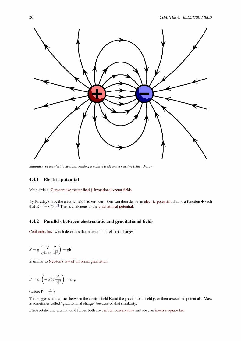
Illustration of the electric field surrounding a positive (red) and a negative (blue) charge.

4.4.1 Electric potential

Main article: Conservative vector field § Irrotational vector fields

By Faraday’s law, the electric field has zero curl. One can then define an electric potential, that is, a function Φ suchthat E = −∇Φ .[3] This is analogous to the gravitational potential.

4.4.2 Parallels between electrostatic and gravitational fields

Coulomb’s law, which describes the interaction of electric charges:

F = q

(Q

4πε0

r̂|r|2)

= qE

is similar to Newton’s law of universal gravitation:

F = m

(−GM

r̂|r|2)

= mg

(where r̂ = r|r| ).

This suggests similarities between the electric field E and the gravitational field g, or their associated potentials. Massis sometimes called “gravitational charge” because of that similarity.Electrostatic and gravitational forces both are central, conservative and obey an inverse-square law.

4.5. ELECTRODYNAMIC FIELDS 27

Electric field between two conductors

4.4.3 Uniform fields

A uniform field is one in which the electric field is constant at every point. It can be approximated by placing twoconducting plates parallel to each other and maintaining a voltage (potential difference) between them; it is only anapproximation because of boundary effects (near the edge of the planes, electric field is distorted because the planedoes not continue). Assuming infinite planes, the magnitude of the electric field E is:

E = −∆ϕ

d

where Δϕ is the potential difference between the plates and d is the distance separating the plates. The negative signarises as positive charges repel, so a positive charge will experience a force away from the positively charged plate, inthe opposite direction to that in which the voltage increases. In micro- and nanoapplications, for instance in relationto semiconductors, a typical magnitude of an electric field is in the order of 106 V⋅m−1, achieved by applying a voltageof the order of 1 volt between conductors spaced 1 µm apart.

4.5 Electrodynamic fields

Main article: Electrodynamics

28 CHAPTER 4. ELECTRIC FIELD

Electrodynamic fields are E-fields which do change with time, for instance when charges are in motion.The electric field cannot be described independently of the magnetic field in that case. If A is the magnetic vectorpotential, defined so that B = ∇× A , one can still define an electric potential Φ such that:

E = −∇Φ− ∂A∂t

One can recover Faraday’s law of induction by taking the curl of that equation

[4]

∇× E = −∂(∇× A)∂t

= −∂B∂t

which justifies, a posteriori, the previous form for E.

4.6 Energy in the electric field

If the magnetic field B is nonzero,The total energy per unit volume stored by the electromagnetic field is[5]

uEM =ε

2|E|2 + 1

2µ|B|2

where ε is the permittivity of the medium in which the field exists, µ its magnetic permeability, and E and B are theelectric and magnetic field vectors.As E and B fields are coupled, it would be misleading to split this expression into “electric” and “magnetic” contribu-tions. However, in the steady-state case, the fields are no longer coupled (see Maxwell’s equations). It makes sensein that case to compute the electrostatic energy per unit volume:

uES =1

2ε|E|2 ,

The total energy U stored in the electric field in a given volume V is therefore

UES =1

2ε

∫V

|E|2 dV ,

4.7 Further extensions

4.7.1 Definitive equation of vector fields

See also: Defining equation (physics) and List of electromagnetism equations

In the presence of matter, it is helpful in electromagnetism to extend the notion of the electric field into three vectorfields, rather than just one:[6]

D = ε0E+ P

whereP is the electric polarization – the volume density of electric dipole moments, andD is the electric displacementfield. Since E and P are defined separately, this equation can be used to define D. The physical interpretation of D isnot as clear as E (effectively the field applied to the material) or P (induced field due to the dipoles in the material),but still serves as a convenient mathematical simplification, since Maxwell’s equations can be simplified in terms offree charges and currents.

4.8. SEE ALSO 29

4.7.2 Constitutive relation

Main article: Constitutive equation

The E and D fields are related by the permittivity of the material, ε.[7][8]

For linear, homogeneous, isotropic materials E and D are proportional and constant throughout the region, there isno position dependence: For inhomogeneous materials, there is a position dependence throughout the material:

D(r) = εE(r)

For anisotropic materials the E and D fields are not parallel, and so E and D are related by the permittivity tensor (a2nd order tensor field), in component form:

Di = εijEj

For non-linear media, E and D are not proportional. Materials can have varying extents of linearity, homogeneityand isotropy.

4.8 See also

• Classical electromagnetism

• Field strength

• signal strength in telecommunications

• Magnetism

• Teltron Tube

• Teledeltos, a conductive paper that may be used as a simple analog computer for modelling fields.

4.9 References

[1] Richard Feynman (1970). The Feynman Lectures on Physics Vol II. Addison Wesley Longman. ISBN 978-0-201-02115-8.

[2] http://public.wsu.edu/~{}jtd/Physics206/michael_faraday.htm

[3] http://physicspages.com/2011/10/08/curl-potential-in-electrostatics/

[4] Huray, Paul G. (2009). Maxwell’s Equations. Wiley-IEEE. p. 205. ISBN 0-470-54276-4.

[5] Introduction to Electrodynamics (3rd Edition), D.J. Griffiths, Pearson Education, Dorling Kindersley, 2007, ISBN 81-7758-293-3

[6] Electromagnetism (2nd Edition), I.S. Grant, W.R. Phillips, Manchester Physics, John Wiley & Sons, 2008, ISBN 978-0-471-92712-9

[7] Electricity and Modern Physics (2nd Edition), G.A.G. Bennet, Edward Arnold (UK), 1974, ISBN 0-7131-2459-8

[8] Electromagnetism (2nd Edition), I.S. Grant, W.R. Phillips, Manchester Physics, John Wiley & Sons, 2008, ISBN 978-0-471-92712-9

30 CHAPTER 4. ELECTRIC FIELD

4.10 External links• Electric field in “Electricity and Magnetism”, R Nave – Hyperphysics, Georgia State University

• 'Gauss’s Law' – Chapter 24 of Frank Wolfs’s lectures at University of Rochester

• 'The Electric Field' – Chapter 23 of Frank Wolfs’s lectures at University of Rochester

• – An applet that shows the electric field of a moving point charge.

• Fields – a chapter from an online textbook

• Learning by Simulations Interactive simulation of an electric field of up to four point charges

• Java simulations of electrostatics in 2-D and 3-D

• Interactive Flash simulation picturing the electric field of user-defined or preselected sets of point charges byfield vectors, field lines, or equipotential lines. Author: David Chappell

Chapter 5

Electric flux

In electromagnetism, electric flux is the measure of flow of the electric field through a given area. Electric flux isproportional to the number of electric field lines going through a normally perpendicular surface. If the electric fieldis uniform, the electric flux passing through a surface of vector area S is

ΦE = E · S = ES cos θ,

where E is the electric field (having units of V/m), E is its magnitude, S is the area of the surface, and θ is the anglebetween the electric field lines and the normal (perpendicular) to S.For a non-uniform electric field, the electric flux dΦE through a small surface area dS is given by

dΦE = E · dS

(the electric field, E, multiplied by the component of area perpendicular to the field). The electric flux over a surfaceS is therefore given by the surface integral:

ΦE =

∫∫S

E · dS

where E is the electric field and dS is a differential area on the closed surface S with an outward facing surface normaldefining its direction.For a closed Gaussian surface, electric flux is given by:

ΦE = S E · dS = Qϵ0

where

E is the electric field,S is any closed surface,Q is the total electric charge inside the surface S,ε0 is the electric constant (a universal constant, also called the "permittivity of free space”) (ε0 ≈ 8.854187 817... x 10−12 farads per meter (F·m−1)).

This relation is known as Gauss’ law for electric field in its integral form and it is one of the four Maxwell’s equations.While the electric flux is not affected by charges that are not within the closed surface, the net electric field, E, inthe Gauss’ Law equation, can be affected by charges that lie outside the closed surface. While Gauss’ Law holds for

31

32 CHAPTER 5. ELECTRIC FLUX

all situations, it is only useful for “by hand” calculations when high degrees of symmetry exist in the electric field.Examples include spherical and cylindrical symmetry.Electrical flux has SI units of volt metres (V m), or, equivalently, newton metres squared per coulomb (N m2 C−1).Thus, the SI base units of electric flux are kg·m3·s−3·A−1.Its dimensional formula is [L3MT−3I−1].

5.1 See also• Magnetic flux

• Maxwell’s equations

related websites are following: http://www.citycollegiate.com/coulomb4_XII.htm[1]

5.2 References[1] electric flux

5.3 External links• Electric flux — HyperPhysics

Chapter 6

Field line

This article is about the modern use of “field lines” as a way to depict electromagnetic and other vector fields. Forthe role of these lines in the early history and philosophy of electromagnetism, see Line of force.A field line is a locus that is defined by a vector field and a starting location within the field. Field lines are useful for

+ -

Field lines depicting the electric field created by a positive charge (left), negative charge (center), and uncharged object (right).

The figure at left shows the electric field lines of two equal positive charges. The figure at right shows the electric field lines of adipole.

visualizing vector fields, which are otherwise hard to depict. Note that, like longitude and latitude lines on a globe, or

33

34 CHAPTER 6. FIELD LINE

topographic lines on a topographic map, these lines are not physical lines that are actually present at certain locations;they are merely visualization tools.

6.1 Precise definition

A vector field defines a direction at all points in space; a field line for that vector field may be constructed by tracinga topographic path in the direction of the vector field. More precisely, the tangent line to the path at each point isrequired to be parallel to the vector field at that point.A complete description of the geometry of all the field lines of a vector field is sufficient to completely specify thedirection of the vector field everywhere. In order to also depict the magnitude, a selection of field lines is drawn suchthat the density of field lines (number of field lines per unit perpendicular area) at any location is proportional to themagnitude of the vector field at that point.As a result of the divergence theorem, field lines start at sources and end at sinks of the vector field. (A “source” iswherever the divergence of the vector field is positive, a “sink” is wherever it is negative.) In physics, drawings offield lines are mainly useful in cases where the sources and sinks, if any, have a physical meaning, as opposed to e.g.the case of a force field of a radial harmonic.For example, Gauss’s law states that an electric field has sources at positive charges, sinks at negative charges, andneither elsewhere, so electric field lines start at positive charges and end at negative charges. (They can also potentiallyform closed loops, or extend to or from infinity, or continuing forever without closing in on itself). A gravitationalfield has no sources, it has sinks at masses, and it has neither elsewhere, gravitational field lines come from infinityand end at masses. A magnetic field has no sources or sinks (Gauss’s law for magnetism), so its field lines have nostart or end: they can only form closed loops, extend to infinity in both directions, or continue indefinitely withoutever crossing itself.Note that for this kind of drawing, where the field-line density is intended to be proportional to the fieldmagnitude, it isimportant to represent all three dimensions. For example, consider the electric field arising from a single, isolated pointcharge. The electric field lines in this case are straight lines that emanate from the charge uniformly in all directionsin three-dimensional space. This means that their density is proportional to 1/r2 , the correct result consistent withCoulomb’s law for this case. However, if the electric field lines for this setup were just drawn on a two-dimensionalplane, their two-dimensional density would be proportional to 1/r , an incorrect result for this situation.[1]

6.2 Examples

If the vector field describes a velocity field, then the field lines follow stream lines in the flow. Perhaps the mostfamiliar example of a vector field described by field lines is the magnetic field, which is often depicted using fieldlines emanating from a magnet.

6.3 Divergence and curl

Field lines can be used to trace familiar quantities from vector calculus:

• Divergence may be easily seen through field lines, assuming the lines are drawn such that the density of fieldlines is proportional to the magnitude of the field (see above). In this case, the divergence may be seen as thebeginning and ending of field lines. If the vector field is the resultant of radial inverse-square law fields withrespect to one or more sources then this corresponds to the fact that the divergence of such a field is zero outsidethe sources. In a solenoidal vector field (i.e., a vector field where the divergence is zero everywhere), the fieldlines neither begin nor end; they either form closed loops, or go off to infinity in both directions. If a vectorfield has positive divergence in some area, there will be field lines starting from points in that area. If a vectorfield has negative divergence in some area, there will be field lines ending at points in that area.

• The Kelvin-Stokes theorem shows that field lines of a vector field with zero curl (i.e., a conservative vectorfield, e.g. a gravitational field or an electrostatic field) cannot be closed loops. In other words, curl is always

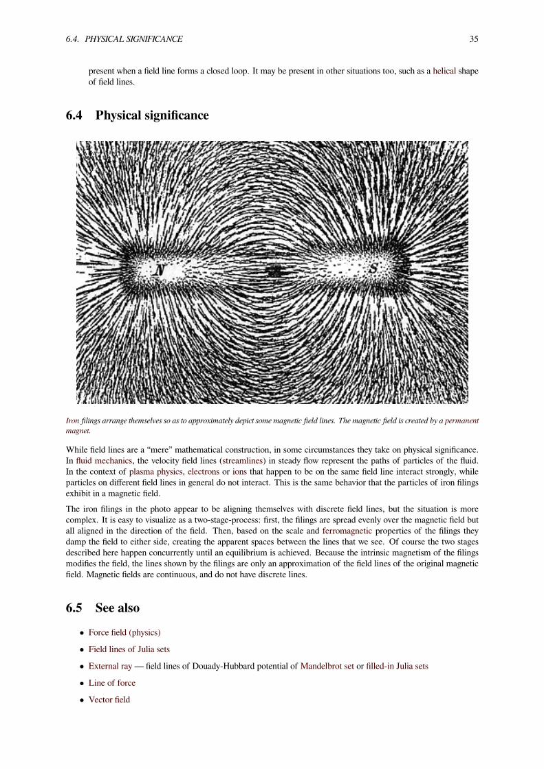
6.4. PHYSICAL SIGNIFICANCE 35

present when a field line forms a closed loop. It may be present in other situations too, such as a helical shapeof field lines.

6.4 Physical significance

Iron filings arrange themselves so as to approximately depict some magnetic field lines. The magnetic field is created by a permanentmagnet.

While field lines are a “mere” mathematical construction, in some circumstances they take on physical significance.In fluid mechanics, the velocity field lines (streamlines) in steady flow represent the paths of particles of the fluid.In the context of plasma physics, electrons or ions that happen to be on the same field line interact strongly, whileparticles on different field lines in general do not interact. This is the same behavior that the particles of iron filingsexhibit in a magnetic field.The iron filings in the photo appear to be aligning themselves with discrete field lines, but the situation is morecomplex. It is easy to visualize as a two-stage-process: first, the filings are spread evenly over the magnetic field butall aligned in the direction of the field. Then, based on the scale and ferromagnetic properties of the filings theydamp the field to either side, creating the apparent spaces between the lines that we see. Of course the two stagesdescribed here happen concurrently until an equilibrium is achieved. Because the intrinsic magnetism of the filingsmodifies the field, the lines shown by the filings are only an approximation of the field lines of the original magneticfield. Magnetic fields are continuous, and do not have discrete lines.

6.5 See also• Force field (physics)• Field lines of Julia sets• External ray — field lines of Douady-Hubbard potential of Mandelbrot set or filled-in Julia sets• Line of force• Vector field

36 CHAPTER 6. FIELD LINE

6.6 References• Griffiths, David J. (1998). Introduction to Electrodynamics (3rd ed.). Prentice Hall. pp. 65–67 and 232. ISBN0-13-805326-X.

• “Visualization of Fields and the Divergence and Curl” course notes from a course at the Massachusetts Instituteof Technology.

[1] A. Wolf, S. J. Van Hook, E. R. Weeks, Electric field line diagrams don't work Am. J. Phys., Vol. 64, No. 6. (1996), pp.714-724 DOI 10.1119/1.18237

6.7 External links• Interactive Java applet showing the electric field lines of selected pairs of charges by Wolfgang Bauer

Chapter 7

Conservative vector field

In vector calculus a conservative vector field is a vector field that is the gradient of some function, known in thiscontext as a scalar potential.[1] Conservative vector fields have the property that the line integral is path independent,i.e. the choice of integration path between any point and another does not change the result. Path independence of aline integral is equivalent to the vector field being conservative. A conservative vector field is also irrotational; in threedimensions this means that it has vanishing curl. An irrotational vector field is necessarily conservative provided thata certain condition on the geometry of the domain holds, i.e. the domain is simply connected.Conservative vector fields appear naturally in mechanics: they are vector fields representing forces of physical systemsin which energy is conserved.[2] For a conservative system, the work done in moving along a path in configurationspace depends only on the endpoints of the path, so it is possible to define a potential energy independently of thepath taken.

7.1 Informal treatment

In a two and three dimensional space, there is an ambiguity in taking an integral between two points as there areinfinitely many paths between the two points - apart from the straight line formed between the two points one couldchoose a curved path of greater length as shown in the figure. Therefore in general the value of the integral depends onthe path taken. However, in the special case of a conservative vector field, the value of the integral is independent ofthe path taken which can be thought of as a large-scale cancellation of all elements dR which don't have a componentalong the straight line between the two points. To visualise this, imagine two people climbing a cliff; one decides toscale the cliff by going vertically up it, and the second decides to walk along a winding path that is longer in length thanthe height of the cliff, but at only a small angle to the horizontal. Although the two hikers have taken different routesto get up to the top of the cliff, at the top they will have both gained the same amount of gravitational potential energy.This is because a gravitational field is conservative. As an example of a non-conservative field, imagine pushing a boxfrom one end of a room to another. Pushing the box in a straight line across the room requires noticeably less workagainst friction than along a curved path covering a greater distance.

7.2 Intuitive explanation

M. C. Escher’s painting Ascending and Descending illustrates a non-conservative vector field, impossibly made toappear to be the gradient of the varying height above ground as one moves along the staircase. It is “rotational” inthat one can keep getting higher or keep getting lower while going around in circles. It is non-conservative in thatone can return to one’s starting point while ascending more than one descends or vice versa. On a real staircase theheight above the ground is a scalar potential field: if one returns to the same place, one goes upward exactly as muchas one goes downward. Its gradient would be a conservative vector field, and is irrotational. The situation depicted inthe painting is impossible.

37

38 CHAPTER 7. CONSERVATIVE VECTOR FIELD

Depiction of two possible paths to integrate. In green in the simplest possible path, blue shows a more convoluted curve

7.3 Definition

A vector field v is said to be conservative if there exists a scalar field φ such that

v = ∇φ.

Here∇φ denotes the gradient of φ . When the above equation holds, φ is called a scalar potential for v .The fundamental theorem of vector calculus states that any vector field can be expressed as the sum of a conservativevector field and a solenoidal field.

7.4 Path independence

Main article: Gradient theorem

A key property of a conservative vector field is that its integral along a path depends only on the endpoints of thatpath, not the particular route taken. Suppose that S ⊆ R3 is a region of three-dimensional space, and that P is arectifiable path in S with start point A and end point B . If v = ∇φ is a conservative vector field then the gradienttheorem states that

7.4. PATH INDEPENDENCE 39

M. C. Escher’s lithograph Ascending and Descending

∫P

v · dr = φ(B)− φ(A).

This holds as a consequence of the chain rule and the fundamental theorem of calculus.An equivalent formulation of this is to say that

40 CHAPTER 7. CONSERVATIVE VECTOR FIELD

∮C

v · dr = 0

for every closed loop C in S. The converse of this statement is also true: if the circulation of v around every closedloop in an open set S is zero, then v is a conservative vector field.

7.5 Irrotational vector fields

The above field v = (−y/(x2 + y2), +x/(x2 + y2), 0) includes a vortex at its center, so it is non-irrotational; it is neither conservative,nor does it have path independence. However, any simply connected subset that excludes the vortex line (0,0,z) will have zero curl,∇ × v = 0. Such vortex-free regions are examples of irrotational vector fields.

A vector field v is said to be irrotational if its curl is zero. That is, if

∇× v = 0.

For this reason, such vector fields are sometimes referred to as curl free field (curl-free vector field) or curl-lessvector fields.It is an identity of vector calculus that for any scalar field φ :

∇×∇φ = 0.

7.6. IRROTATIONAL FLOWS 41

Therefore every conservative vector field is also an irrotational vector field.Provided that S is a simply connected region, the converse of this is true: every irrotational vector field is also aconservative vector field.The above statement is not true if S is not simply connected. Let S be the usual 3-dimensional space, except withthe z -axis removed; that is S = R3 \ {(0, 0, z) | z ∈ R} . Now define a vector field by

v =(

−y

x2 + y2,

x

x2 + y2, 0

).

Then v exists and has zero curl at every point in S ; that is v is irrotational. However the circulation of v around theunit circle in the x, y -plane is equal to 2π . Indeed we note that in polar coordinates v = eϕ/r , so the integral overthe unit circle is equal

∮Cv ·eϕdϕ = 2π . Therefore v does not have the path independence property discussed above,

and is not conservative. (However, in any simply connected subregion of S, it is still true that it is conservative. Infact, the field above is the gradient of arg(x+ iy) . As we know from complex analysis, this is a multi-valued functionwhich requires a branch cut from the origin to infinity to be defined in a continuous way; hence, in a region that doesnot go around the z-axis, its gradient is conservative.)In a simply connected region an irrotational vector field has the path independence property. This can be seen bynoting that in such a region an irrotational vector field is conservative, and conservative vector fields have the pathindependence property. The result can also be proved directly by using Stokes’ theorem. In a connected region anyvector field which has the path independence property must also be irrotational.More abstractly, a conservative vector field is an exact 1-form. That is, it is a 1-form equal to the exterior derivative ofsome 0-form (scalar field) ϕ . An irrotational vector field is a closed 1-form. Since d2 = 0, any exact form is closed,so any conservative vector field is irrotational. The domain is simply connected if and only if its first homology groupis 0, which is equivalent to its first cohomology group being 0. The first de Rham cohomology groupH1

dR is 0 if andonly if all closed 1-forms are exact.

7.6 Irrotational flows

Main article: Vorticity

The flow velocity v of a fluid is a vector field, and the vorticity ω of the flow can be defined by

ω = ∇× v.

A common alternative notation for vorticity is ζ .[3]

If v is irrotational, with ∇× v = 0 , then the flow is said to be an irrotational flow. The vorticity of an irrotationalflow is zero.[4]

Kelvin’s circulation theorem states that a fluid that is irrotational in an inviscid flow will remain irrotational. Thisresult can be derived from the vorticity transport equation, obtained by taking the curl of the Navier-stokes equations.For a two-dimensional flow the vorticity acts as a measure of the local rotation of fluid elements. Note that thevorticity does not imply anything about the global behaviour of a fluid. It is possible for a fluid traveling in a straightline to have vorticity, and it is possible for a fluid which moves in a circle to be irrotational.

7.7 Conservative forces

If the vector field associated to a force F is conservative then the force is said to be a conservative force.The most prominent examples of conservative forces are the force of gravity and the electric field associated to astatic charge. According to Newton’s law of gravitation, the gravitational force, FG , acting on a mass m , due to amassM which is a distance r away, obeys the equation

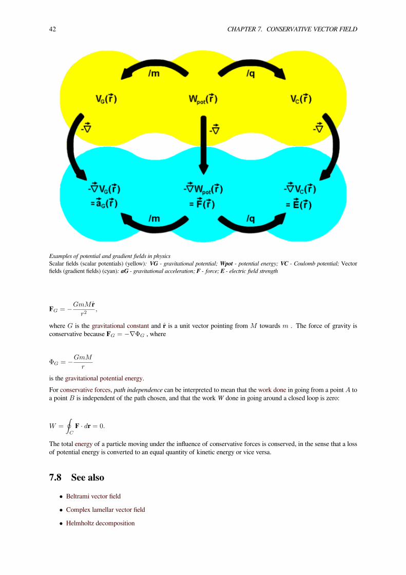
42 CHAPTER 7. CONSERVATIVE VECTOR FIELD

Examples of potential and gradient fields in physicsScalar fields (scalar potentials) (yellow): VG - gravitational potential; Wpot - potential energy; VC - Coulomb potential; Vectorfields (gradient fields) (cyan): aG - gravitational acceleration; F - force; E - electric field strength

FG = −GmM r̂r2

,

where G is the gravitational constant and r̂ is a unit vector pointing from M towards m . The force of gravity isconservative because FG = −∇ΦG , where

ΦG = −GmM

r

is the gravitational potential energy.For conservative forces, path independence can be interpreted to mean that the work done in going from a point A toa point B is independent of the path chosen, and that the workW done in going around a closed loop is zero:

W =

∮C

F · dr = 0.

The total energy of a particle moving under the influence of conservative forces is conserved, in the sense that a lossof potential energy is converted to an equal quantity of kinetic energy or vice versa.

7.8 See also• Beltrami vector field

• Complex lamellar vector field

• Helmholtz decomposition

7.9. CITATIONS AND SOURCES 43

• Laplacian vector field

• Longitudinal and transverse vector fields

• Potential field

• Solenoidal vector field

7.9 Citations and sourcesCitations

[1] Marsden, Jerrold; Tromba, Anthony (2003). Vector calculus (Fifth ed.). W.H.Freedman and Company. pp. 550–561.

[2] George B. Arfken and Hans J. Weber, Mathematical Methods for Physicists, 6th edition, Elsevier Academic Press (2005)

[3] Clancy, L.J., Aerodynamics, Section 7.11, Pitman Publishing Limited, London. ISBN 0-273-01120-0

[4] Liepmann, H.W.; Roshko, A. (1993) [1957], Elements of Gas Dynamics, Courier Dover Publications, ISBN 0-486-41963-0, pp. 194–196.

Sources

• D. J. Acheson, Elementary Fluid Dynamics, Oxford University Press (2005)

Chapter 8

Vector field

A portion of the vector field (sin y, sin x)

In vector calculus, a vector field is an assignment of a vector to each point in a subset of space.[1] A vector field inthe plane, for instance, can be visualized as a collection of arrows with a given magnitude and direction each attachedto a point in the plane. Vector fields are often used to model, for example, the speed and direction of a moving

44

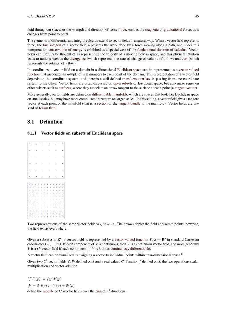
8.1. DEFINITION 45

fluid throughout space, or the strength and direction of some force, such as the magnetic or gravitational force, as itchanges from point to point.The elements of differential and integral calculus extend to vector fields in a natural way. When a vector field representsforce, the line integral of a vector field represents the work done by a force moving along a path, and under thisinterpretation conservation of energy is exhibited as a special case of the fundamental theorem of calculus. Vectorfields can usefully be thought of as representing the velocity of a moving flow in space, and this physical intuitionleads to notions such as the divergence (which represents the rate of change of volume of a flow) and curl (whichrepresents the rotation of a flow).In coordinates, a vector field on a domain in n-dimensional Euclidean space can be represented as a vector-valuedfunction that associates an n-tuple of real numbers to each point of the domain. This representation of a vector fielddepends on the coordinate system, and there is a well-defined transformation law in passing from one coordinatesystem to the other. Vector fields are often discussed on open subsets of Euclidean space, but also make sense onother subsets such as surfaces, where they associate an arrow tangent to the surface at each point (a tangent vector).More generally, vector fields are defined on differentiable manifolds, which are spaces that look like Euclidean spaceon small scales, but may have more complicated structure on larger scales. In this setting, a vector field gives a tangentvector at each point of the manifold (that is, a section of the tangent bundle to the manifold). Vector fields are onekind of tensor field.

8.1 Definition

8.1.1 Vector fields on subsets of Euclidean space

Two representations of the same vector field: v(x, y) = −r. The arrows depict the field at discrete points, however,the field exists everywhere.

Given a subset S in Rn, a vector field is represented by a vector-valued function V: S → Rn in standard Cartesiancoordinates (x1, ..., xn). If each component ofV is continuous, thenV is a continuous vector field, and more generallyV is a Ck vector field if each component of V is k times continuously differentiable.A vector field can be visualized as assigning a vector to individual points within an n-dimensional space.[1]

Given two Ck-vector fields V,W defined on S and a real valued Ck-function f defined on S, the two operations scalarmultiplication and vector addition

(fV )(p) := f(p)V (p)

(V +W )(p) := V (p) +W (p)

define the module of Ck-vector fields over the ring of Ck-functions.

46 CHAPTER 8. VECTOR FIELD

8.1.2 Coordinate transformation law

In physics, a vector is additionally distinguished by how its coordinates change when one measures the same vectorwith respect to a different background coordinate system. The transformation properties of vectors distinguish avector as a geometrically distinct entity from a simple list of scalars, or from a covector.Thus, suppose that (x1,...,xn) is a choice of Cartesian coordinates, in terms of which the components of the vector Vare

Vx = (V1,x, . . . , Vn,x)

and suppose that (y1,...,yn) are n functions of the xi defining a different coordinate system. Then the components ofthe vector V in the new coordinates are required to satisfy the transformation law

Such a transformation law is called contravariant. A similar transformation law characterizes vector fields in physics:specifically, a vector field is a specification of n functions in each coordinate system subject to the transformation law(1) relating the different coordinate systems.Vector fields are thus contrasted with scalar fields, which associate a number or scalar to every point in space, andare also contrasted with simple lists of scalar fields, which do not transform under coordinate changes.

8.1.3 Vector fields on manifolds

Given a differentiable manifold M, a vector field on M is an assignment of a tangent vector to each point in M.[2]More precisely, a vector field F is a mapping fromM into the tangent bundle TM so that p◦F is the identity mappingwhere p denotes the projection from TM to M. In other words, a vector field is a section of the tangent bundle.If the manifoldM is smooth or analytic—that is, the change of coordinates is smooth (analytic)—then one can makesense of the notion of smooth (analytic) vector fields. The collection of all smooth vector fields on a smooth manifoldM is often denoted by Γ(TM) or C∞(M,TM) (especially when thinking of vector fields as sections); the collection ofall smooth vector fields is also denoted by X(M) (a fraktur “X”).

8.2 Examples

• A vector field for the movement of air on Earth will associate for every point on the surface of the Earth avector with the wind speed and direction for that point. This can be drawn using arrows to represent the wind;the length (magnitude) of the arrow will be an indication of the wind speed. A “high” on the usual barometricpressure map would then act as a source (arrows pointing away), and a “low” would be a sink (arrows pointingtowards), since air tends to move from high pressure areas to low pressure areas.

• Velocity field of a moving fluid. In this case, a velocity vector is associated to each point in the fluid.

• Streamlines, Streaklines and Pathlines are 3 types of lines that can be made from vector fields. They are :

streaklines — as revealed in wind tunnels using smoke.streamlines (or fieldlines)— as a line depicting the instantaneous field at a given time.pathlines — showing the path that a given particle (of zero mass) would follow.

• Magnetic fields. The fieldlines can be revealed using small iron filings.

• Maxwell’s equations allow us to use a given set of initial conditions to deduce, for every point in Euclideanspace, a magnitude and direction for the force experienced by a charged test particle at that point; the resultingvector field is the electromagnetic field.

• A gravitational field generated by any massive object is also a vector field. For example, the gravitational fieldvectors for a spherically symmetric body would all point towards the sphere’s center with the magnitude of thevectors reducing as radial distance from the body increases.

8.2. EXAMPLES 47

x

y

z

A vector field on a sphere

8.2.1 Gradient field

Vector fields can be constructed out of scalar fields using the gradient operator (denoted by the del: ∇).[3]

A vector field V defined on a set S is called a gradient field or a conservative field if there exists a real-valuedfunction (a scalar field) f on S such that

V = ∇f =

(∂f

∂x1,∂f

∂x2,∂f

∂x3, . . . ,

∂f

∂xn

).

The associated flow is called the gradient flow, and is used in the method of gradient descent.The path integral along any closed curve γ (γ(0) = γ(1)) in a conservative field is zero:

∮γ

⟨V (x), dx⟩ =∮γ

⟨∇f(x), dx⟩ = f(γ(1))− f(γ(0)).

where the angular brackets and comma: ⟨, ⟩ denotes the inner product of two vectors (strictly speaking – the integrandV(x) is a 1-form rather than a vector in the elementary sense).[4]

8.2.2 Central field

A C∞-vector field over Rn \ {0} is called a central field if

48 CHAPTER 8. VECTOR FIELD

The flow field around an airplane is a vector field in R3, here visualized by bubbles that follow the streamlines showing a wingtipvortex.

V (T (p)) = T (V (p)) (T ∈ O(n,R))

where O(n, R) is the orthogonal group. We say central fields are invariant under orthogonal transformations around0.The point 0 is called the center of the field.Since orthogonal transformations are actually rotations and reflections, the invariance conditions mean that vectorsof a central field are always directed towards, or away from, 0; this is an alternate (and simpler) definition. A centralfield is always a gradient field, since defining it on one semiaxis and integrating gives an antigradient.

8.3 Operations on vector fields

8.3.1 Line integral

Main article: Line integral

A common technique in physics is to integrate a vector field along a curve, i.e. to determine its line integral. Givena particle in a gravitational vector field, where each vector represents the force acting on the particle at a given pointin space, the line integral is the work done on the particle when it travels along a certain path.The line integral is constructed analogously to the Riemann integral and it exists if the curve is rectifiable (has finitelength) and the vector field is continuous.Given a vector field V and a curve γ parametrized by [a, b] (where a and b are real) the line integral is defined as

∫γ

⟨V (x), dx⟩ =∫ b

a

⟨V (γ(t)), γ′(t) dt⟩.

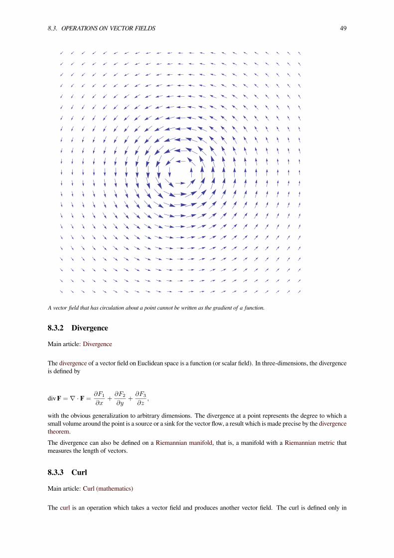
8.3. OPERATIONS ON VECTOR FIELDS 49

A vector field that has circulation about a point cannot be written as the gradient of a function.

8.3.2 Divergence

Main article: Divergence

The divergence of a vector field on Euclidean space is a function (or scalar field). In three-dimensions, the divergenceis defined by

divF = ∇ · F =∂F1

∂x+

∂F2

∂y+

∂F3

∂z,

with the obvious generalization to arbitrary dimensions. The divergence at a point represents the degree to which asmall volume around the point is a source or a sink for the vector flow, a result which is made precise by the divergencetheorem.The divergence can also be defined on a Riemannian manifold, that is, a manifold with a Riemannian metric thatmeasures the length of vectors.

8.3.3 Curl

Main article: Curl (mathematics)

The curl is an operation which takes a vector field and produces another vector field. The curl is defined only in

50 CHAPTER 8. VECTOR FIELD

three-dimensions, but some properties of the curl can be captured in higher dimensions with the exterior derivative.In three-dimensions, it is defined by

curl F = ∇× F =

(∂F3

∂y− ∂F2

∂z

)e1 −

(∂F3

∂x− ∂F1

∂z

)e2 +

(∂F2

∂x− ∂F1

∂y

)e3.

The curl measures the density of the angular momentum of the vector flow at a point, that is, the amount to whichthe flow circulates around a fixed axis. This intuitive description is made precise by Stokes’ theorem.

8.3.4 Index of a vector field

The index of a vector field is a way of describing the behaviour of a vector field around an isolated zero (i.e. non-singular point) which can distinguish saddles from sources and sinks. Take a small sphere around the zero so that noother zeros are included. A map from this sphere to a unit sphere of dimensions n − 1 can be constructed by dividingeach vector by its length to form a unit length vector which can then be mapped to the unit sphere. The index of thevector field at the point is the degree of this map. The index of the vector field is the sum of the indices of each zero.The index will be zero around any non singular point, it is +1 around sources and sinks and −1 around saddles. Intwo dimensions the index is equivalent to the winding number. For an ordinary sphere in three dimension space itcan be shown that the index of any vector field on the sphere must be two, this leads to the hairy ball theorem whichshows that every such vector field must have a zero. This theorem generalises to the Poincaré–Hopf theorem whichrelates the index to the Euler characteristic of the space.

8.4 History

Magnetic field lines of an iron bar (magnetic dipole)

Vector fields arose originally in classical field theory in 19th century physics, specifically in magnetism. They wereformalized by Michael Faraday, in his concept of lines of force, who emphasized that the field itself should be anobject of study, which it has become throughout physics in the form of field theory.

8.5. FLOW CURVES 51

In addition to the magnetic field, other phenomena that were modeled as vector fields by Faraday include the electricalfield and light field.

8.5 Flow curves

Main article: Integral curve

Consider the flow of a fluid through a region of space. At any given time, any point of the fluid has a particularvelocity associated with it; thus there is a vector field associated to any flow. The converse is also true: it is possibleto associate a flow to a vector field having that vector field as its velocity.Given a vector field V defined on S, one defines curves γ(t) on S such that for each t in an interval I

γ′(t) = V (γ(t)) .

By the Picard–Lindelöf theorem, if V is Lipschitz continuous there is a unique C1-curve γx for each point x in S sothat

γx(0) = x

γ′x(t) = V (γx(t)) (t ∈ (−ε,+ε) ⊂ R).The curves γx are called flow curves of the vector field V and partition S into equivalence classes. It is not alwayspossible to extend the interval (−ε, +ε) to the whole real number line. The flow may for example reach the edge of Sin a finite time. In two or three dimensions one can visualize the vector field as giving rise to a flow on S. If we dropa particle into this flow at a point p it will move along the curve γp in the flow depending on the initial point p. If p isa stationary point of V then the particle will remain at p.Typical applications are streamline in fluid, geodesic flow, and one-parameter subgroups and the exponential map inLie groups.

8.5.1 Complete vector fields

A vector field is complete if its flow curves exist for all time.[5] In particular, compactly supported vector fields ona manifold are complete. If X is a complete vector field on M, then the one-parameter group of diffeomorphismsgenerated by the flow along X exists for all time.

8.6 Difference between scalar and vector field

The difference between a scalar and vector field is not that a scalar is just one number while a vector is severalnumbers. The difference is in how their coordinates respond to coordinate transformations. A scalar is a coordinatewhereas a vector can be described by coordinates, but it is not the collection of its coordinates.

8.6.1 Example 1

This example is about 2-dimensional Euclidean space (R2) where we examine Euclidean (x, y) and polar (r, θ)coordinates (which are undefined at the origin). Thus x = r cos θ and y = r sin θ and also r2 = x2 + y2, cos θ = x/(x2+ y2)1/2 and sin θ = y/(x2 + y2)1/2. Suppose we have a scalar field which is given by the constant function 1, and avector field which attaches a vector in the r-direction with length 1 to each point. More precisely, they are given bythe functions

spolar : (r, θ) 7→ 1, vpolar : (r, θ) 7→ (1, 0).

52 CHAPTER 8. VECTOR FIELD

Let us convert these fields to Euclidean coordinates. The vector of length 1 in the r-direction has the x coordinatecos θ and the y coordinate sin θ. Thus in Euclidean coordinates the same fields are described by the functions

sEuclidean : (x, y) 7→ 1,

vEuclidean : (x, y) 7→ (cos θ, sin θ) =(

x√x2 + y2

,y√

x2 + y2

).

We see that while the scalar field remains the same, the vector field now looks different. The same holds even in the1-dimensional case, as illustrated by the next example.

8.6.2 Example 2

Consider the 1-dimensional Euclidean space R with its standard Euclidean coordinate x. Suppose we have a scalarfield and a vector field which are both given in the x coordinate by the constant function 1,

sEuclidean : x 7→ 1, vEuclidean : x 7→ 1.

Thus, we have a scalar field which has the value 1 everywhere and a vector field which attaches a vector in thex-direction with magnitude 1 unit of x to each point.Now consider the coordinate ξ := 2x. If x changes one unit then ξ changes 2 units. But since we wish the integral ofv along a path to be independent of coordinate, this means v*dx=v'*dξ. So from x increase by 1 unit, ξ increases by1/2 unit, so v' must be 2. Thus this vector field has a magnitude of 2 in units of ξ. Therefore, in the ξ coordinate thescalar field and the vector field are described by the functions

sunusual : ξ 7→ 1, vunusual : ξ 7→ 2

which are different.

8.7 f-relatedness

Given a smooth function between manifolds, f: M → N, the derivative is an induced map on tangent bundles, f*:TM → TN. Given vector fields V:M → TM andW : N → TN, we say thatW is f-related to V if the equationW ∘ f*= f* ∘ V holds.If V ᵢ is f-related toW ᵢ, i = 1, 2, then the Lie bracket [V1, V2] is f-related to [W1,W2].

8.8 Generalizations

Replacing vectors by p-vectors (pth exterior power of vectors) yields p-vector fields; taking the dual space and exteriorpowers yields differential k-forms, and combining these yields general tensor fields.Algebraically, vector fields can be characterized as derivations of the algebra of smooth functions on the manifold,which leads to defining a vector field on a commutative algebra as a derivation on the algebra, which is developed inthe theory of differential calculus over commutative algebras.

8.9 See also• Eisenbud–Levine–Khimshiashvili signature formula

• Field line

8.10. REFERENCES 53

• Field strength

• Lie derivative

• Scalar field

• Time-dependent vector field

• Vector fields in cylindrical and spherical coordinates

• Tensor fields

8.10 References[1] Galbis, Antonio & Maestre, Manuel (2012). Vector Analysis Versus Vector Calculus. Springer. p. 12. ISBN 978-1-4614-

2199-3.

[2] Tu, Loring W. (2010). “Vector fields”. An Introduction to Manifolds. Springer. p. 149. ISBN 978-1-4419-7399-3.

[3] Dawber, P.G. (1987). Vectors and Vector Operators. CRC Press. p. 29. ISBN 978-0-85274-585-4.

[4] T. Frankel (2012), The Geometry of Physics (3rd ed.), Cambridge University Press, p. xxxviii, ISBN 978-1107-602601

[5] Sharpe, R. (1997). Differential geometry. Springer-Verlag. ISBN 0-387-94732-9.

8.11 Bibliography• Hubbard, J. H.; Hubbard, B. B. (1999). Vector calculus, linear algebra, and differential forms. A unifiedapproach. Upper Saddle River, NJ: Prentice Hall. ISBN 0-13-657446-7.

• Warner, Frank (1983) [1971]. Foundations of differentiable manifolds and Lie groups. New York-Berlin:Springer-Verlag. ISBN 0-387-90894-3.

• Boothby, William (1986). An introduction to differentiable manifolds and Riemannian geometry. Pure andApplied Mathematics, volume 120 (second ed.). Orlando, FL: Academic Press. ISBN 0-12-116053-X.

8.12 External links• Hazewinkel, Michiel, ed. (2001), “Vector field”, Encyclopedia of Mathematics, Springer, ISBN 978-1-55608-010-4

• Vector field — Mathworld

• Vector field — PlanetMath

• 3D Magnetic field viewer

• Vector fields and field lines

• Vector field simulation An interactive application to show the effects of vector fields

• Vector Fields Software 2d & 3d electromagnetic design software that can be used to visualise vector fields andfield lines

54 CHAPTER 8. VECTOR FIELD

8.13 Text and image sources, contributors, and licenses

8.13.1 Text• Electric charge Source: https://en.wikipedia.org/wiki/Electric_charge?oldid=680302226 Contributors: AxelBoldt, Mav, Andre Engels,

Roadrunner, Peterlin~enwiki, Heron, JohnOwens, Michael Hardy, Ixfd64, Delirium, Looxix~enwiki, Ellywa, Mdebets, Glenn, Rossami,Nikai, Andres, Raven in Orbit, Reddi, Omegatron, Gakrivas, Lumos3, Rogper~enwiki, Gentgeen, Robbot, Fredrik, Dukeofomnium,Wik-ibot, Fuelbottle,Wjbeaty, Giftlite, DavidCary, Herbee, Snowdog, Dratman, Valen~enwiki, RScheiber, JasonQuinn, Brockert, OldakQuill,Manuel Anastácio, LiDaobing, Karol Langner, Icairns, Iantresman, GNU, Vincom2, Discospinster, Guanabot, Jpk, Dbachmann, Ze-roOne, Laurascudder, Bobo192, Rbj, Giraffedata, Kjkolb, Scentoni, Mdd, Alansohn, Atlant, ABCD, Velella, Wtshymanski, HenkvD,Mikeo, DV8 2XL, Gene Nygaard, HenryLi, Oleg Alexandrov, Nuno Tavares, Cimex, Rocastelo, StradivariusTV, Oliphaunt, BillC, Ele-assar777, Cyberman, Palica, BD2412, Demonuk, Edison, SMC, Krash, Dougluce, FlaBot, Psyphen, Nivix, Alfred Centauri, Gurch, Kri,Gdrbot, Manscher, YurikBot, Bambaiah, Lucinos~enwiki, Stephenb, Manop, Pseudomonas, JDoorjam, TDogg310, Chichui, Kkmurray,Wknight94, Light current, Enormousdude, Johndburger, Tcsetattr, Pinikas, Reyk, Canley, Geoffrey.landis, JDspeeder1, GrinBot~enwiki,Mejor Los Indios, Sbyrnes321, Marquez~enwiki, Moeron, Vald, Thunderboltz, Dmitry sychov, HalfShadow, Gilliam, Oscarthecat, AndyM. Wang, Chris the speller, Lenko, DHN-bot~enwiki, Dual Freq, Hallenrm, Rrburke, The tooth, MichaelBillington, Hgilbert, Drphilhar-monic, Daniel.Cardenas, Springnuts, Yevgeny Kats, Andrei Stroe, DJIndica, Naui~enwiki, Nmnogueira, SashatoBot, Richard L. Peterson,Slowmover, Cronholm144, Mgiganteus1, Bjankuloski06en~enwiki, Nonsuch, Ben Moore, RandomCritic, MarkSutton, Stikonas, Dick-lyon, Levineps, Igoldste, Tawkerbot2, Chetvorno, JForget, CmdrObot, Kehrli, Jsd, Myasuda, Cydebot, Fl, Bvcrist, Meno25, Gogo Dodo,WISo, Christian75, Ssilvers, Thijs!bot, Epbr123, Barticus88, N5iln, Mojo Hand, Headbomb, Gerry Ashton, Escarbot, Aadal, AntiVan-dalBot, Seaphoto, Prolog, DarkAudit, Lyricmac, Tim Shuba, WikifingHelper, Asgrrr, JAnDbot, Acroterion, Bongwarrior, VoABot II,J2thawiki, Sstolper, Jjurik, Bubba hotep, User A1, DerHexer, InvertRect, Robin S, MartinBot, M. Bilal Shafiq, LedgendGamer, Pharaohof the Wizards, Numbo3, Hans Dunkelberg, NightFalcon90909, Uncle Dick, Ginsengbomb, Katalaveno, DarkFalls, NewEnglandYankee,QuickClown, Juliancolton, ACBest, Treisijs, Lseixas, Jefferson Anderson, Sheliak, Philip Trueman, TXiKiBoT, The Original Wildbear,Ayan2289, Nickipedia 008, LuizBalloti, Monty845, Jpalpant, Biscuittin, Demmy100, SieBot, Gerakibot, Caltas, Gastin, Wing gundam,Msadaghd, JerrySteal, Jojalozzo, Oxymoron83, Faradayplank, Avnjay, Anchor Link Bot, Neo., Loren.wilton, ClueBot, The Thing ThatShould Not Be, Arakunem, Termine, Mild Bill Hiccup, Stephaninator, LeoFrank, Excirial, Kocher2006, Jusdafax, Brews ohare, Cenar-ium, Jotterbot, PhySusie, SchreiberBike, Wuzur, JDPhD, Versus22, Thinking Stone, Rror, Cernms, Truthnlove, Addbot, Some jerk onthe Internet, CanadianLinuxUser, NjardarBot, LaaknorBot, Scottyferguson, LinkFA-Bot, Naidevinci, Ocwaldron, Tide rolls, Lightbot,JDSperling, Legobot, Luckas-bot, Yobot, CinchBug, Duping Man, AnomieBOT, DemocraticLuntz, Sertion, Jim1138, IRP, Pyrrhus16,Kingpin13, Bluerasberry, Materialscientist, Geek1337~enwiki, ImperatorExercitus, Xqbot, TheAMmollusc, Phazvmk, Addihockey10,Capricorn42, Nnivi, ProtectionTaggingBot, RibotBOT, Srr712, A. di M., Constructive editor, Frozenevolution, Ryryrules100, Jc3s5h,Drunauthorized, Mìthrandir, Steve Quinn, Davidteng, Fast kartwheels, BenzolBot, DivineAlpha, AstaBOTh15, Pinethicket, Jivee Blau,Calmer Waters, Tinton5, MastiBot, Serols, Meaghan, Lalrang2007, Logical Gentleman, FoxBot, TobeBot, SchreyP, Jonkerz, Ndkartik,Vrenator, Taytaylisious09, Ammodramus, Jamietw, DARTH SIDIOUS 2, Eshmate, Irfanyousufdar, EmausBot, John of Reading, Going-Batty, K6ka, Darkfight, Hhhippo, JSquish, Harddk, Stephen CWells, LiamMcM, Sonygal, L Kensington, Donner60, Peter Karlsen, SvenManguard, Planetscared, ClueBot NG, Jack Greenmaven, Cking1414, Ihwood, Ulflund, CocuBot, MelbourneStar, O.Koslowski, Brick-mack, AvocatoBot, Rm1271, Altaïr, F=q(E+v^B), Snow Blizzard, Brad7777, Bhaskarandpm, Eduardofeld, GoShow, Dexbot, JoshyyP,Brandonsmacgregor, Reeceyboii, Frosty, Reatlas, I am One of Many, Eyesnore, Tentinator, Germeten, Nablacdy, Spyglasses, Freddy-boi69, 20M030810, SpecialPiggy, Marizperoj, Peterfreed, Rigid hexagon, Jiteshkumar727464, Dyeith, Podayeruma, Oleaster, Layfi,BlueDecker, GeneralizationsAreBad, Pritam kumar Barik, KasparBot, Ramprakashsfc and Anonymous: 425

• Electrostatic induction Source: https://en.wikipedia.org/wiki/Electrostatic_induction?oldid=646442405Contributors: Heron, Xanzzibar,Giftlite, Superborsuk, ELApro, LeeHunter, Bobo192, Bert Hickman, Alansohn, MiaowMiaow, Prashanthns, Jeff.hochberg@verizon.net,Bgwhite, YurikBot, Plhofmei, E2mb0t~enwiki, BOT-Superzerocool, SmackBot, Incnis Mrsi, Dethme0w, Dogears, Hgrobe, Chetvorno,Christian75, Epbr123, Jj137, JAnDbot, VoABot II, Dekimasu, Email4mobile, Teol~enwiki, VolkovBot, Shindo9Hikaru, ARUNKU-MAR P.R, Enviroboy, Dustybunny, SieBot, Firefly322, WikipedianMarlith, Iohannes Animosus, Addbot, TStein, PV=nRT, Zorrobot,HerculeBot, PieterJanR, Luckas-bot, TaBOT-zerem, AnomieBOT,Xqbot, Robert9673, RedBot, Ezhuttukari, RjwilmsiBot, John of Read-ing, K6ka, JSquish, Ida Shaw, EWikist, Teapeat, Planetscared, ClueBot NG, Helpful Pixie Bot, Fylbecatulous, Fepeguinux, Lugia2453,Monkbot, Gfraz, Sania.qamar15 and Anonymous: 53

• Coulomb’s law Source: https://en.wikipedia.org/wiki/Coulomb’{}s_law?oldid=680669496 Contributors: Andre Engels, Peterlin~enwiki,Heron, Ryguasu, Patrick, Michael Hardy, Ixfd64, Delirium, Eric119, Looxix~enwiki, Ahoerstemeier, Darkwind, AugPi, Reddi, Choster,The Anomebot, E23~enwiki, David.Monniaux, Slawojarek, Robbot, Rorro, Prara, Kathy T, Giftlite, DocWatson42, Radius, Tom-, Yath,Karol Langner, Maximaximax, Icairns, Edsanville, Safety Cap, Aponar Kestrel, Discospinster, Vsmith, Laurascudder, Rbj, Foobaz, Pokra-jac, Kjkolb, Sam Korn, Jumbuck, Mlessard, Rudchenko, Walkerma, Hdeasy, Gene Nygaard, Redvers, Falcorian, Oleg Alexandrov,MartinSpacek, StradivariusTV, Kzollman, Palica, Mendaliv, MZMcBride, Vegaswikian, The wub, Matt Deres, Pediadeep, Fresheneesz,Srleffler, Chobot, Keko~enwiki, YurikBot, Hairy Dude, Jimp, JabberWok, Wimt, NawlinWiki, Dtrebbien, RUL3R, E2mb0t~enwiki,Leotohill, Aristotle2600, Dna-webmaster, Lazcisco, Searchme, Kelovy, Enormousdude, Sbyrnes321, SmackBot, Jclerman, Mangoe,Ququ, InverseHypercube, KnowledgeOfSelf, Pavlovič, Eskimbot, Jab843, Pedrose, Yamaguchi , Pieter Kuiper, Khoshzaban.m, Com-plexica, AlexDitto, Metacomet, DHN-bot~enwiki, Mona, Fjmustak, Can't sleep, clown will eat me, Metal Militia, V1adis1av, HoofHearted, Drphilharmonic, Justin212k, Ligulembot, Sadi Carnot, DJIndica, Nmnogueira, HDarke, Cronholm144, Mbeychok, Bjanku-loski06en~enwiki, Nonsuch, Tiki God, Enelson, Ckatz, Dicklyon, Mets501, Asdfqwe123, Robin Chen, Tawkerbot2, Nutster, Hedge-fighter, Physic sox, WeggeBot, Danrah, Vttoth, Cydebot, Meno25, Christian75, FastLizard4, Editor at Large, Irigi, Headbomb, Jo-jan, Navigatr85, AntiVandalBot, Luna Santin, Seaphoto, Credema, Steelpillow, JAnDbot, Douga, MER-C, Acroterion, WRonG, Wolf-manSF, =avallone, Causesobad, Dr. Morbius, Rettetast, Leyo, Qrystal, Hans Dunkelberg, JohnPritchard, SimpsonDG, Cpiral, M C Y1008, New Hampshirite, NewEnglandYankee, DorganBot, Treisijs, Lseixas, Yecril, Sheliak, VolkovBot, Jeff G., AlnoktaBOT, Fabbe,Thurth, Oshwah, Kychot, Gwib, Hqb, Broadbot, Psyche825, Andy Dingley, Lian1238, Spinningspark, Ohiostandard, CMBJ, Kbrose,SieBot, Cwkmail, Foosnag, OKBot, Randomblue, ClueBot, RedGav, Avenged Eightfold, Mild Bill Hiccup, DragonBot, Kocher2006,Alexbot, Brews ohare, Jotterbot, PhySusie, Thingg, T68492, Gonfer, Addbot, Stariki, NjardarBot, , Ehrenkater, Lightbot, Janeissfeldt, ו ,.עוזי Zorrobot, Snaily, Luckas-bot, Yobot, TaBOT-zerem, Julia W, THEN WHO WAS PHONE?, Backslash Forwardslash,AnomieBOT, Jim1138, Materialscientist, Joeyjoe10, Citation bot, Xqbot, TinucherianBot II, P99am, GrouchoBot, Vmcbride, Shad-owjams, WaysToEscape, Samwb123, Constructive editor, FrescoBot, Lookang, MrMathematique, Citation bot 1, Elockid, 10metreh,RedBot, Toolnut, IVAN3MAN, Inbamkumar86, TobeBot, SchreyP, Lionaneesh, Popovvk, Unioneagle, Irfanyousufdar, EmausBot, Wik-

8.13. TEXT AND IMAGE SOURCES, CONTRIBUTORS, AND LICENSES 55

itanvirBot, Marcreif, K6ka, ZéroBot, Prayerfortheworld, Quondum, Arussoxyz, Isarra, Jesanj, DASHBotAV, ClueBot NG, Joefrom-randb, Umairhassankhanniazi, Yongtao-Li, BG19bot, Vagobot, Silvrous, Dlituiev, 123957a, Foreverascone, IngenieroLoco, Tomjensen-morgan, Reatlas, Luot, Verreax, Jagdshkn, Wamiq, TQV, Nigellwh, Frank Tiernan, SpecialPiggy, JaconaFrere, Mattdb100, Amortias,Kunino Sagiri, Gdzlg, Crystallizedcarbon, TheCoffeeAddict, Zommuter, NekoKatsun, RedPanda25, Sweepy, CanaDeAlba, Pushpraj99and Anonymous: 305

• Electric field Source: https://en.wikipedia.org/wiki/Electric_field?oldid=680213294Contributors: Andre Engels, Peterlin~enwiki,Waveguy,Heron, Patrick, Michael Hardy, Tim Starling, GameGod, Modster, Dgrant, Looxix~enwiki, Nikai, Smack, Tantalate, Reddi, Omegatron,BenRG, Lumos3, Donarreiskoffer, Robbot, Nizmogtr, Wjbeaty, Giftlite, Herbee, TomViza, Ssd, Mboverload, Uranographer, Pcarbonn,MFNickster, Icairns, AmarChandra, Abdull, Jpk, Mjpieters, Mal~enwiki, Ghitis, Purplefeltangel, El C, Laurascudder, Femto, Smalljim,Shenme, I9Q79oL78KiL0QTFHgyc, Bert Hickman, Larry V, Helix84, Benjah-bmm27, ABCD, Riana, Pion, BRW, Wtshymanski, GeneNygaard, Netkinetic, Oleg Alexandrov, Tariqabjotu, Nuno Tavares, Woohookitty, Linas, Mindmatrix, Linnea, Quadduc, StradivariusTV,Scjessey, Rtdrury, SCEhardt, Pfalstad, Mandarax, Jorunn, Strait, Jpeham, Margosbot~enwiki, Fresheneesz, Srleffler, DVdm, Bgwhite,Spiderboy, Stephenb, Gaius Cornelius, Salsb, Wimt, NawlinWiki, Grafen, T-rex, DomenicDenicola, Aristotle2600, Light current, Enor-mousdude, 2over0, Rdrosson, Anclation~enwiki, Mebden, RG2, FyzixFighter, Sbyrnes321, SmackBot, InverseHypercube, Bomac, Pe-drose, Gilliam, Bluebot, Complexica, Lenko, PureRED, Hongooi, Can't sleep, clown will eat me, Chlewbot, Wikipedia brown, Fuhghet-taboutit, Radagast83, Mwtoews, Xezlec, DJIndica, Nmnogueira, FrozenMan, Ckatz, Frokor, Slakr, Dicklyon, Wjejskenewr, Mfrosz,Courcelles, Ziusudra, JRSpriggs, Tpruane, JForget, Ale jrb, Jackzhp, WeggeBot, Bmk, Funnyfarmofdoom, Scott.medling, Cydebot, Hy-draton31, Bvcrist, Michael C Price, Christian75, Chrislk02, Thijs!bot, Irigi, Headbomb, Second Quantization, Austinenator, Big Bird,Icep, AntiVandalBot, Shirt58, Alphachimpbot, JAnDbot, CosineKitty, Misnardi, Magioladitis, Yurei-eggtart, Bongwarrior, VoABot II,Catslash, Rivertorch, Xanthym, Reinam~enwiki, Edward321, Gludwiczak, DinoBot, Dr. Morbius, TheEgyptian, PrestonH, The Anony-mous One, Peter Chastain, Maurice Carbonaro, St.daniel, AntiSpamBot, Qwerty59, Juliancolton, STBotD, Treisijs, Sodaplayer, Lseixas,Robertirwin22, Idioma-bot, Sheliak, Nasanbat, VolkovBot, Doctorkismet, JohnBlackburne, AlnoktaBOT, Philip Trueman, TXiKiBoT,Cosmic Latte, Hqb, OlavN, SheffieldSteel, Andy Dingley, Antixt, Lian1238, HiDrNick, AlleborgoBot, Relilles~enwiki, EmxBot, SieBot,Spartan, Krawi, Gerakibot, JerrySteal, Bentogoa, OKBot, Onlyonefin, ClueBot, André Neves, WriterListener, EoGuy, Jan1nad, Nnemo,Razimantv, Nayafun, Russell4, Excirial, Muro Bot, Corkgkagj, Tvine, MrDeodorant, ZooFari, Wyatt915, Addbot, Tcncv, Fgnievinski,Fluxbyte, FDT, LaaknorBot, AndersBot, Numbo3-bot, Qmark42, Tide rolls, Zorrobot, Legobot, Luckas-bot, Yobot, Ptbotgourou, Frag-gle81, Sdoregon, KamikazeBot, Qui-Gon Jinn, SwisterTwister, DrTrigon, AnomieBOT, Ipatrol, Geek1337~enwiki, Xqbot, Bdforbes,Renaissancee, DSisyphBot, Raffamaiden, Ruy Pugliesi, RibotBOT, Dreitmen, RGForbes, Atomless, Lookang, Ozhu, Hungryhungar-ian, Hwong557, I dream of horses, Zoidfather, Mekeretrig, Rausch, Gryllida, TobeBot, عقیل ,کاشف SchreyP, TheBFG, Sbgirl54,Ddvche, Vinnyzz, EmausBot, Rokerdud, Immunize, Ajraddatz, Trinibones, Wikipelli, K6ka, Hardestcorest, JSquish, ZéroBot, Quondum,Sonygal, OnePt618, Sahimrobot, Maschen, Benjamink8, Verman1, ClueBot NG, Gareth Griffith-Jones, Jmguerrac, Justlettersandnum-bers, Parcly Taxel, Widr, Ryan Vesey, NuclearEnergy, Helpful Pixie Bot, Culo95, Gracielleannep, Chander, Onewhohelps, Bonginkosizwane, F=q(E+v^B), Ea91b3dd, Pithdillinja, Poilkmn1, Brad7777, Szczureq, IkamusumeFan, SortOfStillCare, BrightStarSky, Dexbot,Webclient101, Cerabot~enwiki, The.ever.kid, Nishant nsp, Frosty, Graphium, Mpov, Jharlanherb, Razibot, Reatlas, DavidLeighEllis,Ciro.Landolfi, Tigraan, Blackbombchu, Shipandreceive, SpecialPiggy, AwesomeEvilGenius, Faekynn, Vieque, Henryalston, Fstevens123,Chevoron, Csemohitagrawal, Qzekrom, Isambard Kingdom and Anonymous: 372

• Electric flux Source: https://en.wikipedia.org/wiki/Electric_flux?oldid=666723079 Contributors: Patrick, Giftlite, Aulis Eskola, MikeRosoft, Wtshymanski, Jamesmcguigan, Fuhghettaboutit, Daniel.Cardenas, Cydebot, Christian75, Headbomb, Altamel, JoergenB, Leyo,Izno, TXiKiBoT, Mathwhiz 29, Philip1201, Prestonmag, MenoBot, Wdwd, Gabriel Vidal Álvarez, Djr32, Alexbot, Eeekster, Bodhisattv-aBot, SilvonenBot, Addbot, Physnix, Lightbot, PV=nRT, Fryed-peach, Achilles750, PieterJanR, Luckas-bot, Yobot, Amirobot, Mate-rialscientist, Xqbot, GrouchoBot, Brayan Jaimes, PigFlu Oink, Deathbeast, RedBot, TobeBot, Ddvche, EmausBot, Dcirovic, ZéroBot,EdoBot, BG19bot, Razibot, Wamiq, थाराक्काड् कौशिक्, Edwinfrancisd and Anonymous: 39

• Field line Source: https://en.wikipedia.org/wiki/Field_line?oldid=648371945Contributors: Patrick, BenFrantzDale, MFNickster, Zowie,Vsmith, Oleg Alexandrov, Waldir, Zbxgscqf, MarSch, Aholtman, Bgwhite, Pmg, RussBot, Petri Krohn, Simxp, Sbyrnes321, SmackBot,Adam majewski, Chris the speller, Hongooi, JRSpriggs, Chetvorno, CBM, Zureks, Magioladitis, EagleFan, Gwern, R'n'B, Martinor,Antixt, Phe-bot, Paolo.dL, Firefly322, Addbot, Daniele Pugliesi, Citation bot, , FrescoBot, Lookang, TheBFG, Specs112, DeanBrettle,Gertbuschmann, Wayne Slam, RockMagnetist, ClueBot NG, Gauravjuvekar, Qxukhgiels and Anonymous: 25

• Conservative vector field Source: https://en.wikipedia.org/wiki/Conservative_vector_field?oldid=679369159Contributors: Hephaestos,Patrick, Michael Hardy, Gabbe, AugPi, Silverfish, Charles Matthews, Reddi, Hao2lian, Sverdrup, MFNickster, Billlion, Spoon!, KeenanPepper, Allen McC.~enwiki, Oleg Alexandrov, MarSch, Mauxb, Acyso, Siddhant, RussBot, Encephalon, Zvika, That Guy, From ThatShow!, SmackBot, Complexica, Kotjze, Terry Bollinger, JRSpriggs, CBM, Thijs!bot, Rabbanis, RebelRobot, Infovarius, Kar.ma, De-monicInfluence, VolkovBot, Larryisgood, Commentor, Ferengi, Geometry guy, AlleborgoBot, Quietbritishjim, Dolphin51, PixelBot,Brews ohare, Wdford, Crowsnest, Hess88, Addbot, Trammel, Ozob, Jasper Deng, ב ,.דניאל PV=nRT, Ptbotgourou, AnomieBOT, NOr-beck, Omnipaedista, Paga19141, FrescoBot, Lookang, Sławomir Biały, Nistra, John of Reading, Slawekb, Hhhippo, Qniemiec, Quon-dum, Scientific29, Helpful Pixie Bot, Jcc2011, Permafrost46, DominicPrice, SantiRich, AlicesWards and Anonymous: 35

• Vector field Source: https://en.wikipedia.org/wiki/Vector_field?oldid=680119384 Contributors: AxelBoldt, Chato, Patrick, Chas zzzbrown, Michael Hardy, Tim Starling, Wshun, TakuyaMurata, Cyp, Stevenj, Andres, Charles Matthews, Reddi, Sbwoodside, Dysprosia,Jitse Niesen, Maximus Rex, Fibonacci, Phys, Jaredwf, MathMartin, Idoneus~enwiki, Tosha, Giftlite, BenFrantzDale, Ævar ArnfjörðBjarmason, DefLog~enwiki, LiDaobing, MFNickster, Hellisp, JohnArmagh, Zowie, Klaas van Aarsen, Rich Farmbrough, ReiVaX, Mdd,Wendell, Oleg Alexandrov, Woohookitty, Linas, Jacobolus, Rjwilmsi, MarSch, HannsEwald, Salix alba, Dergrosse, Mo-Al, FlaBot, Mar-gosbot~enwiki, Alfred Centauri, Chobot, 121a0012, WriterHound, YurikBot, Archelon, Buster79, Mgnbar, Darrel francis, Sbyrnes321,SmackBot, RDBury, Rex the first, Pokipsy76, Silly rabbit, Nbarth, DHN-bot~enwiki, Regford, Daqu, Pen of bushido, Andrei Stroe,Cronholm144, Jim.belk, Dwmalone, FelisSchrödingeris, Thijs!bot, KlausN~enwiki, JAnDbot, Rivertorch, Catgut, Sullivan.t.j, User A1,Martynas Patasius, JaGa, Rickard Vogelberg, R'n'B, TomyDuby, Policron, HyDeckar, Jaimeastorga2000, VolkovBot, LokiClock, Julian IDo Stuff, TXiKiBoT, A4bot, Anonymous Dissident, Michael H 34, Geometry guy, Antixt, SieBot, Soler97, Paolo.dL, JackSchmidt, OK-Bot, 7&6=thirteen, Wikidsp, Addbot, Fgnievinski, Topology Expert, EconoPhysicist, AndersBot, Mattmatt79, Jasper Deng, Zorrobot,Jarble, Snaily, Legobot, Luckas-bot, Naudefjbot~enwiki, AnomieBOT, Ciphers, ArthurBot, Titi2~enwiki, Point-set topologist, Fres-coBot, Lookang, Sławomir Biały, Lost-n-translation, Foobarnix, Tcnuk, Rausch, EmausBot, Fly by Night, Slawekb, Hhhippo, ZéroBot,Qniemiec, Wikfr, Glosser.ca, Sp4cetiger, Helpsome, Wcherowi, Clearlyfakeusername, Snotbot, Frietjes, Mesoderm, Vinícius MachadoVogt, Helpful Pixie Bot, Shivsagardharam, Nawk, MusikAnimal, Cispyre, F=q(E+v^B), ChrisGualtieri, Oxherdn, Creepsevry1out andAnonymous: 76

56 CHAPTER 8. VECTOR FIELD

8.13.2 Images• File:Ambox_important.svg Source: https://upload.wikimedia.org/wikipedia/commons/b/b4/Ambox_important.svg License: Public do-

main Contributors: Own work, based off of Image:Ambox scales.svg Original artist: Dsmurat (talk · contribs)• File:Ascending_and_Descending.jpg Source: https://upload.wikimedia.org/wikipedia/en/6/66/Ascending_and_Descending.jpgLicense:

Fair use Contributors:Official M. C. Escher website Original artist: ?

• File:Bcoulomb.png Source: https://upload.wikimedia.org/wikipedia/commons/0/04/Bcoulomb.png License: Public domain Contribu-tors: http://en.wikipedia.org/wiki/Image:Bcoulomb.png Original artist: ?

• File:Camposcargas.PNG Source: https://upload.wikimedia.org/wikipedia/commons/8/8f/Camposcargas.PNG License: CC-BY-SA-3.0 Contributors: Own work Original artist: http://commons.wikimedia.org/wiki/User:Chanchocan

• File:Cessna_182_model-wingtip-vortex.jpg Source: https://upload.wikimedia.org/wikipedia/commons/c/cd/Cessna_182_model-wingtip-vortex.jpg License: CC-BY-SA-3.0 Contributors: Own work Original artist: BenFrantzDale

• File:Commons-logo.svg Source: https://upload.wikimedia.org/wikipedia/en/4/4a/Commons-logo.svg License: ? Contributors: ? Origi-nal artist: ?

• File:Conservative_fields.png Source: https://upload.wikimedia.org/wikipedia/commons/9/9d/Conservative_fields.png License: CC0Contributors: Own work Original artist: Qniemiec

• File:Copyright-problem.svg Source: https://upload.wikimedia.org/wikipedia/en/c/cf/Copyright-problem.svg License: PD Contribu-tors: ? Original artist: ?

• File:Coulomb.jpg Source: https://upload.wikimedia.org/wikipedia/commons/4/42/Coulomb.jpg License: Public domain Contributors:? Original artist: ?

• File:CoulombsLaw.svg Source: https://upload.wikimedia.org/wikipedia/commons/0/07/CoulombsLaw.svg License: CC BY 3.0 Con-tributors: Self-made by User:Dna-Dennis Original artist: User:Dna-Dennis

• File:Coulombslaw.svg Source: https://upload.wikimedia.org/wikipedia/commons/7/73/Coulombslaw.svg License: CC BY-SA 3.0 Con-tributors: Own work Original artist: IngenieroLoco

• File:Edit-clear.svg Source: https://upload.wikimedia.org/wikipedia/en/f/f2/Edit-clear.svg License: Public domain Contributors: TheTango! Desktop Project. Original artist:The people from the Tango! project. And according to themeta-data in the file, specifically: “Andreas Nilsson, and Jakub Steiner (althoughminimally).”

• File:Electric_Field_Lines.svg Source: https://upload.wikimedia.org/wikipedia/commons/2/2a/Electric_Field_Lines.svg License: CC-BY-SA-3.0 Contributors: Own work Original artist: Nein Arimasen

• File:Electric_field_one_charge_changing.gif Source: https://upload.wikimedia.org/wikipedia/commons/e/ea/Electric_field_one_charge_changing.gif License: CC BY-SA 3.0 Contributors: Own work Original artist: Lookang

• File:Electric_field_point_lines_equipotentials.svg Source: https://upload.wikimedia.org/wikipedia/commons/9/96/Electric_field_point_lines_equipotentials.svg License: Public domain Contributors: Own work Original artist: Sjlegg

• File:Electrical_potential_and_field_lines_between_two_wires.png Source: https://upload.wikimedia.org/wikipedia/commons/f/f3/Electrical_potential_and_field_lines_between_two_wires.png License: CC BY-SA 4.0 Contributors: Own work Original artist: Bret Mul-vey

• File:Electroscope_showing_induction.png Source: https://upload.wikimedia.org/wikipedia/commons/e/ec/Electroscope_showing_induction.png License: Public domain Contributors: Downloaded from <a data-x-rel='nofollow' class='external text' href='http://books.google.com/books?id=gPQWAAAAYAAJ,<span>,&,</span>,pg=PA16'>Sylvanus P. Thompson (1881) Elementary Lessons in Electricity and Mag-netism, MacMillan, New York, p.16, fig. 12</a> Original artist: Sylvanus P. Thompson

• File:Electrostatic_induction.svg Source: https://upload.wikimedia.org/wikipedia/commons/d/d9/Electrostatic_induction.svg License:Public domain Contributors: Own work Original artist: Chetvorno

• File:Electrostatic_induction_experiment.png Source: https://upload.wikimedia.org/wikipedia/commons/5/55/Electrostatic_induction_experiment.png License: Public domain Contributors: Retrieved from <a data-x-rel='nofollow' class='external text' href='http://books.google.com/books?id=sKELAAAAYAAJ,<span>,&,</span>,pg=PA410'>Adolphe Ganot & Edmund Atkinson (1872) Natural Philos-ophy for General Readers and Young Persons, D. Appleton & Co., New York, p.410, fig.314</a>, translated and edited from AdolpheGanot, Cours Élémentaire de Physique Original artist: Adolphe Ganot and Edmund Atkinson

• File:Irrotationalfield.svg Source: https://upload.wikimedia.org/wikipedia/commons/6/6d/Irrotationalfield.svg License: CC BY-SA 3.0Contributors: Own work Original artist: AllenMcC.

• File:Magnet0873.png Source: https://upload.wikimedia.org/wikipedia/commons/5/57/Magnet0873.png License: Public domain Con-tributors: <a data-x-rel='nofollow' class='external text' href='http://books.google.com/books?id=BT8AAAAAYAAJ,<span>,&,</span>,pg=PA242'>NewtonHenry Black, Harvey N. Davis (1913) Practical Physics, The MacMillan Co., USA, p. 242, fig. 200</a> Original artist: Newton HenryBlack

• File:Nuvola_apps_edu_mathematics_blue-p.svg Source: https://upload.wikimedia.org/wikipedia/commons/3/3e/Nuvola_apps_edu_mathematics_blue-p.svg License: GPL Contributors: Derivative work from Image:Nuvola apps edu mathematics.png and Image:Nuvolaapps edu mathematics-p.svg Original artist: David Vignoni (original icon); Flamurai (SVG convertion); bayo (color)

• File:Nuvola_apps_ksim.png Source: https://upload.wikimedia.org/wikipedia/commons/8/8d/Nuvola_apps_ksim.png License: LGPLContributors: http://icon-king.com Original artist: David Vignoni / ICON KING

• File:OiintLaTeX.svg Source: https://upload.wikimedia.org/wikipedia/commons/8/86/OiintLaTeX.svgLicense: CC0Contributors: Ownwork Original artist: Maschen

• File:Paper_shavings_attracted_by_charged_cd.jpg Source: https://upload.wikimedia.org/wikipedia/commons/0/0c/Paper_shavings_attracted_by_charged_cd.jpg License: Public domain Contributors: Own work Original artist: Pediadeep

8.13. TEXT AND IMAGE SOURCES, CONTRIBUTORS, AND LICENSES 57

• File:Pathdependence.png Source: https://upload.wikimedia.org/wikipedia/en/1/1f/Pathdependence.png License: CC0 Contributors:Own workOriginal artist:DominicPrice (talk) (Uploads)

• File:Question_book-new.svg Source: https://upload.wikimedia.org/wikipedia/en/9/99/Question_book-new.svg License: Cc-by-sa-3.0Contributors:Created from scratch in Adobe Illustrator. Based on Image:Question book.png created by User:Equazcion Original artist:Tkgd2007

• File:Radial_vector_field_dense.svg Source: https://upload.wikimedia.org/wikipedia/commons/c/c4/Radial_vector_field_dense.svgLi-cense: Public domain Contributors: Self-made, generated with Mathematica 7.0 Original artist: Connor Glosser

• File:Radial_vector_field_sparse.svg Source: https://upload.wikimedia.org/wikipedia/commons/b/b1/Radial_vector_field_sparse.svgLicense: CC BY-SA 3.0 Contributors: Self-made, generated with Mathematica 7.0 Original artist: Connor Glosser

• File:Text_document_with_red_question_mark.svg Source: https://upload.wikimedia.org/wikipedia/commons/a/a4/Text_document_with_red_question_mark.svg License: Public domain Contributors: Created by bdesham with Inkscape; based upon Text-x-generic.svgfrom the Tango project. Original artist: Benjamin D. Esham (bdesham)

• File:VFPt_charges_plus_minus_thumb.svg Source: https://upload.wikimedia.org/wikipedia/commons/e/ed/VFPt_charges_plus_minus_thumb.svg License: CC BY-SA 3.0 Contributors: This plot was created with VectorFieldPlot Original artist: Geek3

• File:VFPt_image_charge_plane_horizontal.svg Source: https://upload.wikimedia.org/wikipedia/commons/3/37/VFPt_image_charge_plane_horizontal.svg License: CC BY-SA 3.0 Contributors: This plot was created with VectorFieldPlot Original artist: Geek3

• File:VFPt_minus_thumb.svg Source: https://upload.wikimedia.org/wikipedia/commons/d/d7/VFPt_minus_thumb.svg License: CCBY-SA 3.0 Contributors: This plot was created with VectorFieldPlot Original artist: Geek3

• File:VFPt_plus_thumb.svg Source: https://upload.wikimedia.org/wikipedia/commons/9/95/VFPt_plus_thumb.svg License: CC BY-SA 3.0 Contributors: This plot was created with VectorFieldPlot Original artist: Geek3

• File:VectorField.svg Source: https://upload.wikimedia.org/wikipedia/commons/b/b9/VectorField.svg License: Public domain Contrib-utors: Own work Original artist: Jim.belk

• File:Vector_sphere.svg Source: https://upload.wikimedia.org/wikipedia/commons/6/6e/Vector_sphere.svgLicense: CC-BY-SA-3.0Con-tributors: Own work Original artist: Cronholm144

• File:Verificacion_ley_coulomb.png Source: https://upload.wikimedia.org/wikipedia/commons/5/51/Verificacion_ley_coulomb.pngLi-cense: CC-BY-SA-3.0 Contributors: Own work Original artist: http://commons.wikimedia.org/wiki/User:Chanchocan

8.13.3 Content license• Creative Commons Attribution-Share Alike 3.0