electrical signals in a heart - université du littoral

Created in COMSOL Multiphysics 5.4

E l e c t r i c a l S i g n a l s i n a Hea r t

This model is licensed under the COMSOL Software License Agreement 5.4.All trademarks are the property of their respective owners. See www.comsol.com/trademarks.

http://www.comsol.com/sla

http://www.comsol.com/trademarks/

This example was kindly provided by Prof. Simonetta Filippi and Dr Christian Cherubini from Università Campus Biomedico di Roma, Italy.

Introduction

Modeling the electrical activity in cardiac tissue is an important step in understanding the patterns of contractions and dilations in the heart. The heart produces rhythmic electrical pulses, initiated from a point known as the sinus node. The electrical pulses, in turn, trigger the mechanical contractions of the muscle. In a healthy heart these electrical pulses are damped out, but a number of heart conditions involve an elevated risk of re-entry of the signals. This means that the normal steady pulse is disturbed, a severe and acute condition often referred to as arrhythmia.

In this example, different aspects of electrical signal propagation in cardiac tissue are studied using the FitzHugh-Nagumo equations and the Complex Ginzburg-Landau equations, both of which are solved on the same geometry. Interesting patterns emerging from these types of models are, for example, spiral waves, which, in the context of cardiac electrical signals, can produce effects similar to those observed in cardiac arrhythmia.

E X C I T A B L E M E D I A A N D T H E F I T Z H U G H - N A G U M O E Q U A T I O N S

It has been shown that many important characteristics of electrical signal propagation in cardiac tissue can be reproduced by a class of equations which describe excitable media, that is, materials consisting of elementary segments or cells with the following basic characteristics:

• Well-defined rest state

• Threshold for excitation

• A diffusive-type coupling to its nearest neighbors

Excitable media is a rather general concept, which is useful for modeling of a number of different phenomena, including nerve pulses, the spreading of forest fires, and certain types of chemical reactions, in addition to the electrical signals in cardiac tissue. One of the most important qualitative characteristics displayed by excitable media, and equally a common denominator between the diversity of phenomena mentioned above, is the almost immediate damping out of signals below a certain threshold. On the other hand, signals exceeding this threshold propagate without damping.

The heart works by passing ionic current inside the muscle, thus triggering the rhythmic contractions that pump blood in and out. The ions move through small pores or gates in the cellular membrane, which can be either open (excitation state) or closed (rest state).

2 | E L E C T R I C A L S I G N A L S I N A H E A R T

In nerve cells and cardiac cells the three abstract characteristics of excitable media are manifested as:

• Rest cell membrane potential

• Threshold for opening the ionic gates in the cellular membrane

• The diffusive spreading of the electrical signals

The state of the membrane gates is random on a microscopic scale, but the probability of a given state can be modeled as a continuous function of the voltage, thus allowing an averaged macroscopic continuum description of the current flow.

The FitzHugh-Nagumo equations for excitable media describe the simplest physiological model with two variables, an activator and an inhibitor. In these heart models the activator variable corresponds to the electric potential, and the inhibitor is a variable that describes the voltage-dependent probability of the pores in the membrane being open and ready to transmit ionic current.

C H A O T I C D Y N A M I C S A N D T H E C O M P L E X L A N D A U - G I N Z B U R G E Q U A T I O N S

The complex Landau-Ginzburg equations provide a relatively simple way of modeling some aspects of the transition, displayed by many dynamical systems under the influence of strong external stimulus, from periodic oscillatory behavior into a chaotic state with gradually increasing amplitude of oscillations and decreasing periodicity.

Although their first use was to describe the theory of superconductivity, the complex Landau-Ginzburg equations are also generic in their nature (as are the FitzHugh-Nagumo equations), and examples of dynamical systems that you can model successfully using these equations are:

• The formation of vortices behind a slender obstacle in transversal fluid flow

• Oscillating chemical reactions of the Belousov-Zhabotinsky type

In this example, the complex Landau-Ginzburg equations simulate the dynamics of the spiral waves in excitable media.


Model Definition

The geometry here is a simplified 3D model of a heart with two chambers, represented with semispherical cavities1.

Figure 1: Model geometry.

T H E F I T Z H U G H - N A G U M O E Q U A T I O N S

The equations are the following:

Here u1 is an action potential (the activator variable), and u2 is a gate variable (the inhibitor variable). The parameter α represents the threshold for excitation, ε represents the excitability, and β, γ, and δ are parameters that affect the rest state and dynamics of the system.

1. Note that it is possible to import more realistic human/animal heart geometries, with anisotropies and inhomogeneities as well as proper dimensions, into COMSOL Multiphysics using the CAD import capabilities.

t∂∂u1 uΔ α u1–( ) u1 1–( )u1 u2–( )+ +=

t∂∂u2 ε βu1 γu2– δ–( )=


The boundary conditions for u1 are insulating, using the assumption that no current is flowing into or out of the heart. The initial condition defines an initial potential distribution u1 where one quadrant of the heart is at a constant, elevated potential V0, while the rest remains at zero. The adjacent quadrant has instead an elevated value ν0 for the inhibitor u2. It is convenient to implement this initial distribution using the following logical expressions, where TRUE evaluates to 1 and FALSE to 0:

Here d is equal to 10−5, and it is included in the expressions to shift the elevated potential slightly off the main axes.

T H E C O M P L E X L A N D A U - G I N Z B U R G E Q U A T I O N S

The complex Landau-Ginzburg equations are:

The two variables v1 and v2 are the activator and inhibitor, respectively. The constants c1 and c3 are parameters reflecting the properties of the material. These constants also determine the existence and nature of the stable solutions.

As in the previous model, the boundary conditions are kept insulating. The initial condition, which gives a smooth transition step near z = 0, are the following:

Notes About the COMSOL Implementation

The simplified geometry is quite straightforward to create using the drawing tools in COMSOL Multiphysics. The FitzHugh-Nagumo and Landau-Ginzburg equations are also readily entered in one of the PDE interfaces2.

2. With this stage completed, it would also be straightforward to replace the rather simple equations with a physiologically more realistic mathematical model.

u1 0 x y z, , ,( ) V0 x d+( ) 0>( ) z d+( ) 0>( )⋅=

u2 0 x y z, , ,( ) v2 x– d+( ) 0>( ) z d+( ) 0>( )⋅=

t∂∂v1 v1 c1v2–( )Δ– v1 v1 c3v2–( ) v1

2 v22

+( )–=

t∂∂v2 c1v1 v2+( )Δ– v2 c3v1 v2+( ) v1

2 v22

+( )–=

v1 0 x y z, , ,( ) z( )tanh=

v2 0 x y z, , ,( ) z( )tanh–=


It is important to note that these equations are strongly nonlinear. It is therefore necessary (especially in full 3D models like these) to use a much finer mesh or use higher element order than in this example to get results with some degree of reliability for the time intervals of interest. This is particularly important in solving the complex Landau-Ginzburg equations, which describe inherently chaotic phenomena. They are highly sensitive to perturbations in the initial value and similarly to numerical errors during the course of the time-dependent solution. We recommend the use of the fourth-order Hermite element for the complex Landau-Ginzburg equation.

For the reasons above, the results presented here are only intended as a first rough estimate of the qualitative behavior that you can expect the system to show under a given stimulus. Consequently, higher-order elements, finer meshing, and smaller relative and absolute time dependent tolerances clearly give quantitatively more correct simulation results. The implementation of these improvements leads to longer computational time than that for the rough model described here which takes a few minutes to compute on a standard PC. When attempting these types of large models we strongly recommend the use of 64-bit platforms.

To avoid warnings about inconsistent units, turn off unit support.

Results and Discussion

T H E F I T Z H U G H - N A G U M O E Q U A T I O N S

The plots in Figure 2 below show the action potential u1. To visualize the solution on the inside, a quarter of the outside shell of the heart and one of the chamber surfaces are suppressed in the plot.


The parameters used in the model along with the initial pulse lead to a reentrant wave which travels around the tissue without damping in a characteristic spiral pattern.

Figure 2: Solution to the FitzHugh-Nagumo equations at times t = 120 s (top) and t = 500 s (bottom).


T H E L A N D A U - G I N Z B U R G E Q U A T I O N S

Figure 3 below shows the species v1 at different times.

Figure 3: Solution to the Complex Landau-Ginzburg equations at times t = 75 s (top) and t = 45 s (bottom).

The equation parameters and initial condition used here lead the diffusing species (v1) to display characteristic spiral patterns with growing complexity over time.


References

1. F.H. Fenton, E.M. Cherry, H.M. Hastings, and S.J. Evans, “Real-time computer simulations of excitable media: JAVA as a scientific language and as a wrapper for C and FORTRAN programs,” BioSystems, vol. 64, pp. 73–96, 2002.

2. Y. Kuramoto, Chemical Oscillations, Waves and Turbulence, Dover Publications, 2003.

3. J. Keener and J. Sneyd, Mathematical Physiology, Springer, 1998.

Application Library path: COMSOL_Multiphysics/Equation_Based/heart_electrical

Modeling Instructions

From the File menu, choose New.

N E W

In the New window, click Model Wizard.

M O D E L W I Z A R D

1 In the Model Wizard window, click 3D.

2 In the Select Physics tree, select Mathematics>PDE Interfaces>General Form PDE (g).

3 Click Add.

4 In the Number of dependent variables text field, type 2.

5 Click Study.

6 In the Select Study tree, select General Studies>Time Dependent.

7 Click Done.

R O O T

1 In the Model Builder window, click the root node.

2 In the root node’s Settings window, locate the Unit System section.

3 From the Unit system list, choose None.

The equations in this model are given in dimensionless form. Turning off unit support avoids warnings about inconsistent use of units.


G E O M E T R Y 1

Follow the instructions below to recreate the geometry illustrated in Figure 1.

Sphere 1 (sph1)1 In the Geometry toolbar, click Sphere.

2 In the Settings window for Sphere, locate the Size section.

3 In the Radius text field, type 54.

4 Right-click Sphere 1 (sph1) and choose Build Selected.

Ellipsoid 1 (elp1)1 In the Geometry toolbar, click More Primitives and choose Ellipsoid.

2 In the Settings window for Ellipsoid, locate the Size and Shape section.

3 In the a-semiaxis text field, type 54.

4 In the b-semiaxis text field, type 54.

5 In the c-semiaxis text field, type 70.

6 Right-click Ellipsoid 1 (elp1) and choose Build Selected.

Next create the egg-shaped solid by fusing the top half of the sphere with the bottom half of the ellipsoid. Use blocks to remove the bottom half of sphere and the top half of ellipsoid.

Block 1 (blk1)1 In the Geometry toolbar, click Block.

2 In the Settings window for Block, locate the Size and Shape section.

3 In the Width text field, type 110.

4 In the Depth text field, type 110.

5 In the Height text field, type 110.

6 Locate the Position section. From the Base list, choose Center.

7 In the z text field, type 55.

8 Right-click Block 1 (blk1) and choose Build Selected.

Difference 1 (dif1)1 In the Geometry toolbar, click Booleans and Partitions and choose Difference.

2 Select the object elp1 only.

3 In the Settings window for Difference, locate the Difference section.

4 Find the Objects to subtract subsection. Select the Active toggle button.


5 Select the object blk1 only.

6 Right-click Difference 1 (dif1) and choose Build Selected.

Block 2 (blk2)1 In the Geometry toolbar, click Block.

2 In the Settings window for Block, locate the Size and Shape section.

3 In the Width text field, type 110.

4 In the Depth text field, type 110.


6 Locate the Position section. From the Base list, choose Center.

7 In the z text field, type -55.

8 Right-click Block 2 (blk2) and choose Build Selected.


2 Select the object sph1 only.



5 Select the object blk2 only.


Union 1 (uni1)1 In the Geometry toolbar, click Booleans and Partitions and choose Union.

2 Click in the Graphics window and then press Ctrl+A to select both objects.

3 In the Settings window for Union, click Build All Objects.

Now create the cavity inside the heart.

Scale 1 (sca1)1 In the Geometry toolbar, click Transforms and choose Scale.

2 In the Settings window for Scale, locate the Input section.

3 Select the Keep input objects check box.

4 Select the object uni1 only.

5 Locate the Scale Factor section. In the Factor text field, type 2/3.

6 Right-click Scale 1 (sca1) and choose Build Selected.

7 Click the Transparency button in the Graphics toolbar.



2 Select the object uni1 only.



5 Select the object sca1 only.


The next step is to create the wall separating the two chambers.

Cylinder 1 (cyl1)1 In the Geometry toolbar, click Cylinder.

2 In the Settings window for Cylinder, locate the Size and Shape section.

3 In the Radius text field, type 45.


5 Locate the Position section. In the x text field, type -5.

6 In the z text field, type -5.

7 Locate the Axis section. From the Axis type list, choose Cartesian.

8 In the x text field, type 1.

9 In the z text field, type 0.

10 Right-click Cylinder 1 (cyl1) and choose Build Selected.

Union 2 (uni2)1 In the Geometry toolbar, click Booleans and Partitions and choose Union.

2 Click in the Graphics window and then press Ctrl+A to select both objects.

3 In the Settings window for Union, locate the Union section.

4 Clear the Keep interior boundaries check box.

5 Click Build All Objects.

This completes the geometry.

G L O B A L D E F I N I T I O N S

1 In the Model Builder window, under Global Definitions click Parameters 1.

2 In the Settings window for Parameters, locate the Parameters section.


3 In the table, enter the following settings:

Use the default Neumann boundary condition at all the boundaries.

G E N E R A L F O R M P D E ( G )

General Form PDE 11 In the Model Builder window, under Component 1 (comp1)>General Form PDE (g) click

General Form PDE 1.

2 In the Settings window for General Form PDE, locate the Conservative Flux section.

3 Specify the second Γ vector as

4 Locate the Source Term section. In the f text-field array, type (alpha-u1)*(u1-1)*u1-u2 on the first row.

5 In the f text-field array, type epsilon*(beta*u1-gamma*u2-delta) on the second row.

Initial Values 11 In the Model Builder window, under Component 1 (comp1)>General Form PDE (g) click

Initial Values 1.

2 In the Settings window for Initial Values, locate the Initial Values section.

3 In the u1 text field, type V0*((x+d)>0)*((z+d)>0).

4 In the u2 text field, type nu0*((-x+d)>0)*((z+d)>0).

Name Expression Value Description

alpha 0.1 0.1 Excitation threshold

epsilon 0.01 0.01 Excitability

beta 0.5 0.5 System parameter

gamma 1 1 System parameter

delta 0 0 System parameter

V0 1 1 Elevated potential value

nu0 0.3 0.3 Elevated inhibitor value

d 1e-5 1E-5 Off-axis shift distance

0 x

0 y

0 z


M E S H 1

1 In the Model Builder window, under Component 1 (comp1) click Mesh 1.

2 In the Settings window for Mesh, locate the Physics-Controlled Mesh section.

3 From the Element size list, choose Fine.

4 Click Build All.

S T U D Y 1

Step 1: Time Dependent1 In the Model Builder window, under Study 1 click Step 1: Time Dependent.

2 In the Settings window for Time Dependent, locate the Study Settings section.

3 In the Times text field, type range(0,5,500).

4 In the Home toolbar, click Compute.

R E S U L T S

3D Plot Group 1The default plot shows a slice plot of the dependent variable. To create plots given in Figure 2, you need to suppress some of the boundaries.


Study 1/Solution 1 (sol1)1 In the Model Builder window, expand the Results>Data Sets node.

2 Right-click Study 1/Solution 1 (sol1) and choose Selection.

Selection1 In the Model Builder window, under Results>Data Sets>Study 1/Solution 1 (sol1) click

Selection.

2 In the Settings window for Selection, locate the Geometric Entity Selection section.

3 From the Geometric entity level list, choose Boundary.

4 Click Paste Selection.

5 In the Paste Selection dialog box, type 1 3 10-18 in the Selection text field.

6 Click OK.


8 Click Create Selection.

9 In the Create Selection dialog box, click OK.

3D Plot Group 21 In the Home toolbar, click Add Plot Group and choose 3D Plot Group.

2 In the Settings window for 3D Plot Group, locate the Plot Settings section.

3 Clear the Plot data set edges check box.

Surface 11 Right-click 3D Plot Group 2 and choose Surface.

2 In the 3D Plot Group 2 toolbar, click Plot.

3 Click the Transparency button in the Graphics toolbar.

3D Plot Group 21 In the Model Builder window, under Results click 3D Plot Group 2.

2 In the Settings window for 3D Plot Group, locate the Data section.

3 From the Time (s) list, choose 120.


This completes the modeling of the FitzHugh-Nagumo equations. To model the Complex Landau-Ginzburg equations use the following set of instructions.

A D D P H Y S I C S

1 In the Home toolbar, click Add Physics to open the Add Physics window.


2 Go to the Add Physics window.

3 In the tree, select Mathematics>PDE Interfaces>General Form PDE (g).

4 Click to expand the Dependent Variables section. In the Field name text field, type v.

5 In the Number of dependent variables text field, type 2.

6 In the Dependent variables table, enter the following settings:

7 Find the Physics interfaces in study subsection. In the table, clear the Solve check box for Study 1.

8 Click Add to Component in the window toolbar.

9 In the Home toolbar, click Add Physics to close the Add Physics window.

A D D S T U D Y

1 In the Home toolbar, click Add Study to open the Add Study window.

2 Go to the Add Study window.

3 Find the Studies subsection. In the Select Study tree, select General Studies>Eigenvalue.

4 Find the Physics interfaces in study subsection. In the table, clear the Solve check box for the General Form PDE (g) interface.

5 Find the Studies subsection. In the Select Study tree, select General Studies>

Time Dependent.

6 Click Add Study in the window toolbar.

7 In the Home toolbar, click Add Study to close the Add Study window.

G L O B A L D E F I N I T I O N S

1 In the Settings window for Parameters, locate the Parameters section.

2 In the table, enter the following settings:

G E N E R A L F O R M P D E 2 ( G 2 )

The accuracy of the soultion can be improved by using cubic Hermite elements instead of the default quadratic Lagrange elements.

1 In the Model Builder window, under Component 1 (comp1) click General Form PDE 2 (g2).

v1

Name Expression Value Description

c1 2 2 PDE parameter

c3 -0.2 -0.2 PDE parameter


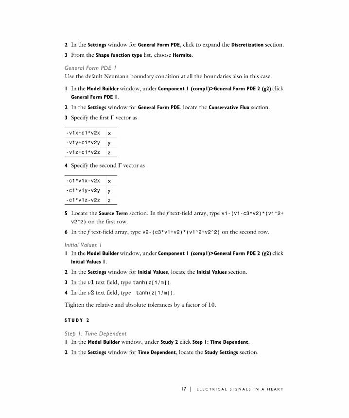
2 In the Settings window for General Form PDE, click to expand the Discretization section.

3 From the Shape function type list, choose Hermite.

General Form PDE 1Use the default Neumann boundary condition at all the boundaries also in this case.

1 In the Model Builder window, under Component 1 (comp1)>General Form PDE 2 (g2) click General Form PDE 1.

2 In the Settings window for General Form PDE, locate the Conservative Flux section.

3 Specify the first Γ vector as

4 Specify the second Γ vector as

5 Locate the Source Term section. In the f text-field array, type v1-(v1-c3*v2)*(v1^2+v2^2) on the first row.

6 In the f text-field array, type v2-(c3*v1+v2)*(v1^2+v2^2) on the second row.

Initial Values 11 In the Model Builder window, under Component 1 (comp1)>General Form PDE 2 (g2) click

Initial Values 1.

2 In the Settings window for Initial Values, locate the Initial Values section.

3 In the v1 text field, type tanh(z[1/m]).

4 In the v2 text field, type -tanh(z[1/m]).

Tighten the relative and absolute tolerances by a factor of 10.

S T U D Y 2

Step 1: Time Dependent1 In the Model Builder window, under Study 2 click Step 1: Time Dependent.

2 In the Settings window for Time Dependent, locate the Study Settings section.

-v1x+c1*v2x x

-v1y+c1*v2y y

-v1z+c1*v2z z

-c1*v1x-v2x x

-c1*v1y-v2y y

-c1*v1z-v2z z


3 In the Times text field, type range(0,5,75).

4 From the Tolerance list, choose User controlled.

5 In the Relative tolerance text field, type 0.001.

6 In the Study toolbar, click Show Default Solver.

Solution 2 (sol2)1 In the Model Builder window, expand the Solution 2 (sol2) node, then click Time-

Dependent Solver 1.

2 In the Settings window for Time-Dependent Solver, click to expand the Absolute Tolerance section.

3 From the Tolerance method list, choose Manual.

4 In the Absolute tolerance text field, type 0.0001.

5 In the Study toolbar, click Compute.

R E S U L T S

Follow the instructions to create plots given in Figure 3.

Study 2/Solution 2 (sol2)In the Model Builder window, under Results>Data Sets right-click Study 2/Solution 2 (sol2) and choose Selection.

Selection1 In the Model Builder window, under Results>Data Sets>Study 2/Solution 2 (sol2) click

Selection.


3 From the Geometric entity level list, choose Boundary.

4 From the Selection list, choose Explicit 1.

3D Plot Group 41 In the Home toolbar, click Add Plot Group and choose 3D Plot Group.


3 From the Data set list, choose Study 2/Solution 2 (sol2).

4 Locate the Plot Settings section. Clear the Plot data set edges check box.

Surface 11 Right-click 3D Plot Group 4 and choose Surface.


2 In the Settings window for Surface, click Replace Expression in the upper-right corner of the Expression section. From the menu, choose Component 1>General Form PDE 2>v1 - Dependent variable v1.


3D Plot Group 41 In the Model Builder window, under Results click 3D Plot Group 4.


3 From the Time (s) list, choose 45.



electrical signals in a heart - université du littoral

Documents