elasticities of substitution - economics:...

Elasticities of Substitution

R. Robert RussellUniversity of California, Riverside

[email protected]

Draft (October 2017)

Abstract

This draft chapter, prepared for inclusion in the (prospective) Handbookof Production Economics, Vol. 1 (Theory), edited by Subash Ray, RobertChambers, and Subal Kumbhakar, lays out the theoretical foundation ofthe measurement of the degree of substitutability among inputs utilized ina production process. It proceeds from the well-settled (Hicksian) notionof this measure for two inputs (typically labor and capital) to the morechallenging conceptualization for technologies with more than two inputs(most notably, Allen-Uzawa and Morishima elasticities). Dual elastici-ties of substitution (also called elasticities of complementary) and grosselasticities of substitution (measuring substitutability for non-homothetictechnologies taking account of output changes) are also covered. Also an-alyzed are functional representations of two-input technologies with con-stant elasticity of substitution (CES) and of n-input technologies withconstant and identical elasticities for all pairs of inputs. Finally, the chap-ter explores the relationship between elasticity values and the compara-tive statics of factor income shares and the relationships between certainelasticity identities and separability conditions rationalizing consistent ag-gregation of subsets of inputs.

1

Chapter 4

Elasticities of Substitution

R. Robert Russell

4.1 Introduction.

In his classic book on the Theory of Wages, the Oxford University economistJohn R. Hicks [1932] introduced two concepts that persist to this day asimportant components of both microeconomic and macroeconomic analysis:(1) elasticity of substitution1 and (2) input neutrality (alternatively, inputbias) of technological change. Each of these constructs is fundamental to theanalysis of changing factor income shares as an economy (or other productionunit) expands (or, for that matter, contracts). This chapter focuses on thefirst of these concepts; Chapter 5 covers the second.

As noted by Blackorby and Russell [1989, p. 882] in their discussion of theelasticity of substitution, “Hicks’ key insight was to note that [in a two-factoreconomy] the effect of changes in the capital/labor ratio (or the factor priceratio) on the distribution of income (for a given output) can be completelycharacterized by a scalar measure of curvature of the isoquant.”2 This mea-

1The concept was independently formulated by Cambridge University economist JoanRobinson [1933] in her comparably classic book on The Economics of Imperfect Compe-tition. Abba Lerner [1933] and A. C. Pigou [1934] also contributed to the understandingof the concept at its genesis.

2While the use of the word “curvature” in this quote conveys the appropriate intuition,

1

2 CHAPTER 4. ELASTICITIES OF SUBSTITUTION

sure, the (two-input) elasticity of substitution, is a logarithmic derivative ofthe input-quantity ratio with respect to the technical rate of substitution be-tween the two inputs, holding output constant. The elasticity of substitutionand its relationship to the comparative statics of income shares is expositedin Section 4.2, where the famous SMAC (Arrow, Chenery, Minhaus, andSolow [1961]) theorem on the functional characterization of constancy of theelasticity of substitution (CES) is also discussed.

Generalization of the elasticity of substitution to allow for more than twoinputs began with suggestions by Hicks and Allen [1934]. One suggestionwas to employ the constructions defining the original Hicksian notion for anytwo inputs, holding the other input quantities fixed. This idea was furtherexplored by McFadden [1963], but since then it has faded from the picture,largely because its failure to allow for optimal adjustment of other inputsmeans that it generally fails to provide information about the comparativestatics of relative income shares of any two inputs.3

The other generalization formulated by Hicks and Allen [1934]—and fur-ther analyzed by Hicks [1938], Allen [1938], and Uzawa [1962]—is now knownas the Allen elasticity of substitution (AES) or the Allen-Uzawa elasticity ofsubstitution (AUES). This elasticity is a share-weighted (constant-output)cross elasticity of demand. An alternative generalization, first formulatedby Morishima [1967] (in Japanese and unfortunately never translated intoEnglish) and independently discovered by Blackorby and Russell [1975], isa constant-output cross elasticity of demand minus a constant-output ownprice elasticity of demand.4 Blackorby and Russell [1981] named this conceptthe “Morishima elasticity of substitution” (MES) and argued that it, unlikethe AES, preserves the salient properties of the original Hicksian notion when

it is nevertheless technically incorrect, in part because curvature, formally defined, is aunit-dependent mathematical concept. See de la Grandville [1997] for a clear expositionof this point.

3As pointed out by Blackorby and Russell [1981, p. 882], “[O]nly if the two variableswere separable from all other variables would [this elasticity] provide information aboutshares; if we were to require all pairs to have this property, the production function wouldbe additive. When combined with homotheticity (an assumption maintained in all thesestudies . . . ) this implies that the production function is CES, in which case [the elasticities]are constant for all pairs of inputs.”

4The Morishima elasticity is a generalization of Robinson’s [1933] characterization ofthe two-input elasticity and for this reason is called the “Robinson elasticity of substitutionby Kuga and Murota [1972] and Kuga [1979].

4.1. INTRODUCTION. 3

the number of inputs is expanded to more than two. As these (and other)elasticity concepts are most evocatively described using dual representationsof the technology, Section 4.3 presents some useful duality constructs. Fea-tures of the AES and the MES are then explored in Section 4.4, particularlytheir relationships to the comparative statics of factor income shares andfunctional representations of the technology when the elasticities are invari-ant with respect to changes in input quantities.

The curvature of a two-input isoquant can be equivalently (and againinformally) represented by the inverse of the Hicksian elasticity, the logarith-mic derivative of the technical rate of substitution—i.e., the shadow priceratio—with respect to the quantity ratio. These concepts are dual to oneanother. Of course, in the case of only two variables, these two elasticitiesare simple inverses of one another (and have inverse implications for the cur-vature of the isoquant). With more than two inputs, however, the analogousdual concepts—duals to the Allen and Morishima elasticities—are not sim-ple inverses of one another. This dual structure, developed by Blackorby andRussell [1975, 1981], is examined in Section 4.5.2.

Stern [2010] points out that the dual Morishima elasticities do not reflectdifferential movements along an isoquant (essentially because only one inputis varied in the calculation). He proposes an elasticity, named the symmetricsymmetric elasticity of complementarity, that constrains differential changesin quantities to be contained in an isoquant. This elasticity, unlike the dualMorishima elasticity, is symmetric.5 It is presented in Section 4.5.3.

The Allen and Morishima elasticities of substitution are calculated fordifferential movements along a constant-output surface. If the technology ishomothetic, this is not a restriction, but in general the comparative-staticcalculations on, say, income shares hold only for cases where outputs areexogenous. The extension of the Allen elasticity to incorporate output effectswas broached by Mundlak [1968] and formulated in the dual (using the profitfunction) by Lau [1978]. Extensions of these results to Morishima elasticitiescan be found in Davis and Shumway [1996] and Blackorby, Primont, andRussell [2007]. In line with the latter, I refer to these concepts as grosselasticities and describe and analyze them in Section 4.6.

In a widely cited paper, Berndt and Christensen [1973] were the first to

5It is dual, not to the Morishima elasticity, but to McFadden’s [1963] shadow elasticityof substitution.


notice that identities among certain pairs of Allen elasticities are equivalentto corresponding separability restrictions on the production function. Es-sentially, a set of inputs is separable from a distinct input if the technicalrates of substitution among inputs in the set are independent of the quantityof the excluded input. Separability is a powerful concept in part because ithas implications for the possibility of consistent aggregation of inputs (ı.e.,aggregation across different types of labor inputs to form an aggregate inputin the functional representation of the technology).6 If a subset of inputs isseparable from all inputs excluded from the subset, there exists an aggre-gator over the inputs in the subset, which then is an aggregate input intothe production function. Berndt and Christensen discovered that a subset ofinputs is separable from a distinct input if and only if the Allen elasticitiesof substitution between the excluded and each of the inputs in the separablesubset are identical. Russell [1975] and Blackorby and Russell [1976, 1981]later generalized these results and extended them to comparable identityrestrictions for Morishima elasticities of substitution. These relationshipsbetween certain elasticity identities and functional structure are covered inSection 4.7.

Chapter 4.8 concludes with allusions to the extensive literature in whichthe elasticity of substitution plays a salient role.

4.2 Two-Input Elasticity of Substitution: Early

Formulations and Characterizations.

4.2.1 Definition.

Hicks was particularly interested in the substitutability between labor andcapital, and more particularly in the relative income shares of these twoinputs. Let us therefore denote the input quantity vector, in an obviousnotation, by 〈x`, xk〉 ∈ R2

+ and the (scalar) output quantity by y ∈ R+. Theproduction function, F : R2

+ → R+, is assumed to be increasing, strictly

6Separability is also a necessary condition for decentralization of an optimization prob-lem (as in, e.g., two-stage budgeting). See Blackorby, Primont, and Russell [1978] fora thorough exposition of the connection between separability and decentralized decisionmaking.

4.2. TWO-INPUT ELASTICITY OF SUBSTITUTION: EARLY FORMULATIONS AND CHARACTERIZATIONS.5

quasi-concave, and homothetic.7 For convenience, we restrict our analysis tothe interior of quantity space, R2

++, and assume that F is continuously twicedifferentiable on this space.8

Homotheticity of F implies that the technical rate of substitution betweenlabor and capita,9

trs`,k = F`(x`, xk)/Fk(x`, xk) =: TRS`,k(x`, xk),

is homogeneous of degree zero, so that

trs`,k = TRS`,k(1, xk/x`) =: t(xk/x`)

andln trs`,k = ln t(xk/x`) =: θ( ln(xk/x`)).

Owing to strict quasi-concavity of F , t is strictly monotonic, hence invertible,and we can write

xkx`

= t−1(trs`,k)

orlnxkx`

=: φ(ln trs`,k).

The (two-input) elasticity of substitution is defined as the log derivativeof the input-quantity ratio with respect to the technical rate of substitution,

σ = φ′(ln trs`,k),

or, equivalently, as the inverse of the log derivative of the technical rate ofsubstitution with respect to the input-quantity ratio,

σ =1

θ′( ln(xk/x`)).

7As we shall see in Section 3, the homotheticity assumption can be dropped when theelasticity concept is formulated in the dual.

8We could extend our analysis to all of R2+ by employing directional derivatives at the

boundary but instead leave this technical detail to the interested reader.9Subscripts on functions indicate differentiation with respect to the specified variable.

The relation, =, should be interpreted as an identity throughout this chapter i.e., asholding for all allowable values of the variables). Also, A := B means the relation definesA, and A =: B means the relation defines B.


As the production function is strictly concave, the elasticity of substitu-tion lies in the open interval, (0,∞). Relatively large values of σ indicatethat the rate at which one input can be substituted for the other is relativelyinsensitive to changes in the input ratio: in the vernacular, substitution is“relatively easy” (isoquants are “relatively flat”). Conversely, lower valuesof σ reflect “relatively difficult” substitution (and “strong curvature” of iso-quants). As σ →∞, the isoquants converge to (parallel) linear line segments(perfect substitution), and as σ → 0, the isoquants converge to Leontief(fixed proportions) isoquants.

4.2.2 Comparative Statics of Income Shares.

As shown by Hicks [1932], the value of the elasticity of substitution hasunambiguous implications for the effects of changes in relative factor pricesor in relative factor quantities on relative factor shares in a competitive (pricetaking) economy. In an obvious notation for factor prices, the share of capitalrelative to labor is s = pkxk/p`x`. In a competitive economy, where trs`,k =p`/pk,

ln s = ln(xk/x`)− ln(p`/pk)

= φ( ln(p`/pk))− ln(p`/pk) =: S(ln(p`/pk)),

= ln(xk/x`)− θ( ln(xk/x`)) =: S(ln(xk/x`)),

so that the proportional effect on relative shares of a change in the price ratiois

S ′( ln(p`/pk)) = φ′( ln(p`/pk))− 1 = σ − 1

and the proportional effect on relative shares of a change in the quantityratio is

S ′( ln(xk/x`)) = 1− θ′( ln(xk/x`)) = 1− 1

σ.

Thus, the comparative statics of functional income shares when σ is constantis encapsulated in

d S(ln(p`/pk))

d ln(p`/pk)

<=>

1 ⇐⇒ σ

<=>

1

4.2. TWO-INPUT ELASTICITY OF SUBSTITUTION: EARLY FORMULATIONS AND CHARACTERIZATIONS.7

or

d S(ln(xk/x`))

d ln(xk/x`))

<=>

1 ⇐⇒ σ

>=<

1.

4.2.3 Constant Elasticity of Substitution.

Implicit in Hicks’s analysis of substitutability is the assumption that the elas-ticity is constant for all values of the input vector. This begs the question ofthe restrictiveness of this assumption, a question that later was answered byArrow, Chenery, Minhas, and Solow [1961] (affectionately known as SMACin much of the literature). Assuming that the technology is convex and ho-mogeneous of degree one, they showed that the elasticity of substitution isconstant (independent of xk/x`) if and only if

F (x`, xk) =(α`x

ρ` + αkx

ρk

)1/ρ

, 1 ≥ ρ 6= 0, (CES2)

orF (x`, xk) = γxα` x

1−αk , γ > 0, 1 > α > 0. (CD2)

Thus, constancy of the elasticity of substitution implies that the produc-tion function must be belong to the CES family of technologies, (CES2) or(CD2).

10 Moreover, the fixed-proportions technology (Leontief [1953]) is gen-erated as a limiting case of (CES2):

limρ→−∞

(α`x

ρ` + αkx

ρk

)1/ρ

= min {α`x`, αkxk}. (L2)

Some simple calculations show that (CES2) ⇐⇒ σ = 1/(1− ρ), (CD2)⇐⇒σ = 1; and (L2) ⇐⇒ σ → 0.11

10The Cobb-Douglas production function was well known at the time of the SMACderivation, having been proposed much earlier (Cobb and Douglas [1928]). The (CES2)production function made its first appearance in Solow’s [1956] classic economic growthpaper, but the functional form had appeared much earlier in the context of utility theory:Bergson (Burk) [1936] proved that additivity of the utility function and linear Engel curves(expenditures on individual goods proportional to income for given prices) implies that theutility function belongs to the CES family. As the SMAC authors point out, the function(CES2) itself was long known in the functional-equation literature (see Hardy, Littlewood,and Polya [1934, p. 13]) as the “mean value of order ρ”.

11The SMAC theorem is easily generalized to homothetic technologies, in which case theproduction function is a monotonic transformation of (CES2) or (CD2); in the limitingcase as σ → 0 it is a monotonic transformation of (L2).


I need not bring to the attention of the reader the extent to which theCES family of production functions has been, over the years, a perennialworkhorse in both theoretical and empirical research employing productionfunctions.

4.3 Digression: Dual Representations of Multiple-

Input, Multiple-Output Technologies.

The Allen and Morishima elasticities, originally formulated by Hicks andAllen [1934] and Morishima [1967] in the (primal) context of a single-outputproduction function, are more generally and evocatively exposited in the dual(using the cost function) as first shown, respectively, by Uzawa [1962]12 andby Blackorby and Russell [1975, 1981], Kuga [1979], and Kuga and Murota[1972]. The dual approach also allows us to move seamlessly from technolo-gies with a single output to those with multiple outputs. Finally, dualitytheory is needed for the development of the dual elasticities of substitutionin Section 4.5. This section lays out the requisite duality theory.13

Denote the ordered set of inputs by N = 〈1, . . . n〉 and the ordered set ofoutputs by M = 〈1, . . .m〉. Input and output quantity vectors are denotedx ∈ Rn

+ and y ∈ Rm+ , respectively. The technology set is the set of all feasible

〈input, output〉 combinations:

T := {〈x, y〉 ∈ Rn+m+ | x can produce y}.

While the nomenclature suggests that feasibility is a purely technologicalnotion, a more expansive interpretation is possible: feasibility could incor-porate notions of institutional and political constraints, especially when weconsider entire economies as the basic production unit.

An input requirement set for a fixed output vector y is

L(y) := {x ∈ Rn+ | 〈x, y〉 ∈ T}.

12Because the Allen elasticities are now typically exposited in the dual, they are oftencalled the “Allen-Uzawa elasticities,” and we resort to that nomenclature on occasion aswell. Uzawa’s approach was later extended by Blackorby and Russell [1975, 1981].

13Thorough expositions of duality theory can be found in, e.g., Blackorby, Primont, andRussell [1978], Chambers [1988], Cornes [1992], Diewert [1974, 1982], Fare and Primont[1995], Fuss and McFadden [1978], and Russell [1997].

4.3. DIGRESSION: DUAL REPRESENTATIONS OFMULTIPLE-INPUT, MULTIPLE-OUTPUT TECHNOLOGIES.9

We assume throughout that, for all y ∈ Rm+ , L(y) is closed and strictly convex

(relative to Rn+)14 and satisfies strong input disposability

L(y) = L(y) + Rn+ ∀ y ∈ Rm

+ ,

output monotonicity,15

y > y ⇒ L(y) ⊂ L(y),

and “no free lunch”,y 6= 0(m) ⇒ 0(n) /∈ L(y).

The (input) distance (gauge) function, a mapping from16

Q := {〈x, y〉 ∈ Rn+m+ | y 6= 0(m) ∧ x 6= 0(n) ∧ L(y) 6= ∅}

into the positive real line (where 0(n) is the null vector of Rn+), is defined by

D(x, y) := max {λ | x/λ ∈ L(y)}.

Under the above assumptions, D is well defined on this restricted domainand satisfies homogeneity of degree one, positive monotonicity, concavity, andcontinuity in x, and negative monotonicity in y. (See, e.g., Fare and Primont[1995] for proofs of these properties and most of the duality results thatfollow.17) Assume, in addition, that D is continuously twice differentiable inx. The distance function is a representation of the technology, since (underour assumptions)

〈x, y〉 ∈ T ⇐⇒ D(x, y) ≥ 1.

In the single-output case (m = 1), where the technology can be repre-sented by a production function, F : Rn

+ → R+, D(x, F (x)) = 1 and the

14These assumptions are stronger than needed for much of the conceptual developmentthat follows, but in the interest of simplicity I maintain them throughout.

15Vector notation: y ≥ y if yj ≥ yj for all j; y > y if yj ≥ yj for all j and y 6= y; andy � y if yj > yj for all j.

16We restrict the domain of the distance function to assure that it is globally welldefined. An alternative approach (e.g., Fare and Primont [1995]) is to define D on theentire non-negative (n + m)-dimensional Euclidean space and replace “max” with “sup”in the definition. See Russell [1997, footnote 12] for a comparison of these approaches.

17Whatever is not there can be found in Diewert [1974, ] or the Fuss/McFadden [1978]volume.


production function is recovered by inverting D(x, y) = 1 in y. If (and onlyif) the technology is homogeneous of degree one (constant returns to scale),

D(x, y) =F (x)

y.

The cost function, C : Rn++ × Y → R+, where

Y = {y | 〈x, y〉 ∈ Q for some x},

is defined byC(p, y) = min

x{p · x | x ∈ L(y)}

or, equivalently, by

C(y, p) = minx{p · x | D(x, y) ≥ 1}. (4.1)

Under our maintained assumptions, D is recovered from C by

D(x, y) = infp{p · x | C(p, y) ≥ 1}, (4.2)

and C has the same properties in p as D has in x. This establishes theduality between the distance and the cost function. On the other hand, Cis positively monotonic in y. We also assume that C is twice continuouslydifferentiable in p.

By Shephard’s Lemma (application of the envelope theorem to (4.1), the(vector-valued, constant-output) input demand function, δ : Rn

++×Y → Rn+,

is generated by first-order differentiation of the cost function:18

δ(p, y) = ∇pC(p, y).

Of course, δ is homogeneous of degree zero in p. The (normalized) shadow-price vector, ρ : Q → R+, is obtained by applying the envelope theorem to(4.2):

ρ(x, y) = ∇xD(x, y). (4.3)

As is apparent from the re-writing of (4.2) (using homogeneity of C in p) as

D(x, y) = infp/c

{pc· x | C(p/c, y) ≥ 1

}= inf

p/c

{pc· x | C(p, y) ≥ c

},

18∇pC(p, y) := 〈∂C(p, y)/∂p1, . . . , ∂C(p, y)/∂pn〉.

4.4. ALLEN AND MORISHIMA ELASTICITIES OF SUBSTITUTION.11

where c can be interpreted as (minimal) expenditure (to produce output y)and the vector ρ(x, y) in (4.3) can be interpreted as shadow prices normalizedby minimal cost.19 In other words, under the assumption of cost-minimizingbehavior,

ρ(δ(p, y), y) =p

C(p, y).

Clearly, ρ is homogeneous of degree zero in x.

4.4 Allen and Morishima Elasticities of Sub-

stitution.

4.4.1 Allen Elasticities of Substitution (AES).

The Allen elasticity of substitution between inputs i and j, is given by

σAij(p, y) : =C(p, y)Cij(p, y)

Ci(p, y)Cj(p, y)(4.4)

=εij(p, y)

sj(p, y), (4.5)

where the subscripts on the cost function C indicate differentiation withrespect to the indicated variable(s);

εij(p, y) :=∂ ln δi(p, y)

∂ ln pj=pjCij(p, y)

Ci(p, y).

is the (constant-output) elasticity of demand for input i with respect to achange in the price of input j; and

sj(p, y) =pjδj(p, y)

C(p, y)=pjCj(p, y)

C(p, y)

is the cost share of input j. Thus, the Allen elasticity is simply a share-weighted cross (i 6= j) or own (i = j) demand elasticity. It collapses to theHicksian elasticity when n = 2.

19See Fare and Grosskopf [1994] and Russell [1997] for analyses of the distance functionand associated shadow prices.


4.4.2 Morishima Elasticities of Substitution (MES).

To define the Morishima elasticities, let pi be the (n− 1)-dimensional vectorof price ratios with pi in the denominator. Zero-degree homogeneity of δ inp allows us to write

δ(pi, y) := δ(p, y).

The Morishima elasticity of substitution of input i for input j is defineddirectly as

σMij (p, y) :=∂ ln

(δi(p

i, y) / δj(pi, y)

)∂ ln(pj/pi)

. (4.6)

Note that any variation in a single component of pi, say pj′/pi, holdingother components (j 6= j′) constant, must be entirely manifested in variationin pj′ alone. Hence, for all pairs 〈i, j〉,

∂δi(pi, y)

∂(pj/pi)=∂δi(p, y)

∂pj

1

pi.

Using this fact, along with Shephard’s Lemma, the MES can be re-writtenin the dual as

σMij (p, y) = pj

(Cij(p, y)

Ci(p, y)− Cjj(p, y)

Cj(p, y)

)(4.7)

= εij(p, y)− εjj(p, y). (4.8)

Thus, the MES is simply the difference between the appropriate (constant-output) cross price elasticity of demand and the (constant-output) own elas-ticity of demand for the input associated with the axis along which the priceratio is being varied.

The Morishima elasticity, unlike the Allen elasticity, is non-symmetric,since the value depends on the normalization adopted in (4.6)—that is, onthe coordinate direction in which the prices are varied to change the priceratio, pj/pi

20 Of course, if there are only two inputs, there is no differencebetween changing pi and changing pj, and the MES, like the AES, collapsesto the standard Hicksian elasticity. But in the general n-input case, the

20See Blackorby and Russell [1975, 1981, 1989] for a discussion of this asymmetry, which(as pointed out by Stern [2011]) was recognized much earlier by Pigou [1934] in his analysisof Robinson’s [1933] less-formal characterization of this elasticity concept.


interactions between these two inputs is dependent on whether it is one orthe other that is varied.21

4.4.3 AES and MES and the Comparative Statics ofIncome Shares.

If σAij(p, y) > 0 (that is, if increasing the jth price increases the optimalquantity of input i), we say that inputs i and j are Allen-Uzawa substitutes;if σAij(p, y) < 0, they are Allen-Uzawa complements. Similarly, if σMij (p, y) > 0(that is, if increasing the jth price increases the optimal quantity of input irelative to the optimal quantity of input j), we say that input j is a Morishimasubstitute for input i; if σMij (p, y) < 0, input j is a Morishima complementto input i. As the Morishima elasticity of substitution is non-symmetric, sois the taxonomy of Morishima substitutes and complements.22

The conceptual foundations of Allen-Uzawa and Morishima taxonomiesof substitutes and complements are, of course, quite different. The Allen-Uzawa taxonomy classifies a pair of inputs as substitutes (complements) ifan increase in the price of one causes an increase (decrease) in the quan-tity demanded of the other. This is the standard textbook definition of netsubstitutes (and complements). The Morishima concept, on the other hand,classifies a pair of inputs as substitutes (complements) if an increase in theprice of one causes the quantity of the other to increase (decrease) relativeto the quantity of the input for which price has changed. For this reason, theMorishima taxonomy leans more toward substitutability (since the theoret-ically necessary decrease in the denominator of the quantity ratio in (4.6)(owing to εjj(p, y) < 0) helps the ratio to decline when the price of the inputin the denominator increases).

Put differently, if two inputs are substitutes according to the Allen-Uzawacriterion, theoretically they must be substitutes according to the Morishimacriterion, but if two inputs are complements according to the Allen-Uzawa

21“Own” Morishima elasticities are identically equal to zero and hence uninteresting, asone might expect to be the case for a sensible elasticity of substitution.

22These notions are referred to as “p-substitutes” and “p-complements” in much ofthe literature (see Stern [2011] and the papers cited there), as distinguished from “q-substitutes” and “q-complements”, which I call dual substitutes and complements in Sec-tion 4.5.


criterion, they can be either complements or substitutes according to theMorishima criterion. This relationship can be seen algebraically from (4.5)and (4.8) . If i and j are Allen-Uzawa substitutes, in which case εij(p, y) > 0,concavity of the cost function (and hence negative semi-definiteness of thecorresponding Hessian) implies that εij(p, y) − εjj(p, y) > 0, so that j is aMorishima substitute for i. Similar algebra establishes that two inputs canbe Morishima substitutes when they are Allen-Uzawa complements.

Note that, for i 6= j,

∂ ln si(p, y)

∂ ln pj= εij(p, y)− sj(p, y) = sj(p, y)(σAij(p, y)− 1),

so that an increase in pj increases the absolute cost share of input i if andonly if σAij(p, y) > 1; that is, if and only if inputs i and j are sufficientlystrong net substitutes. Thus, the Allen-Uzawa elasticities provide immediatequalitative comparative-static information about the effect of price changeson absolute shares. To obtain quantitative comparative-static information,one needs to know the share of the jth input as well as the Allen-Uzawaelasticity of substitution.

The Morishima elasticities immediately yield both qualitative and quan-titative information about the effect of price changes on relative input shares:

∂ ln(si(pi, y)/sj(p

i, y))

∂ ln(pj/pi)= εij(p, y)− εjj(p, y)− 1 = σMij (p, y)− 1,

where (with the use of zero-degree homogeneity of si in p) si(pi, y) := si(p, y)

for all i. Thus, an increase in pj increases the share of input i relative toinput j if and only if

σMij (p, y) > 1;

that is, if and only if inputs i and j are sufficiently substitutable in the senseof Morishima. Moreover, the degree of departure of the Morishima elasticityfrom unity provides immediate quantitative information about the effect onthe relative factor shares.


4.4.4 Constancy of the Allen and Morishima Elastici-ties.

In addition to his dual reformulation of the elasticity proposed by Hicks andAllen [1934], Uzawa [1962] also extended the SMAC theorem on constancyof the elasticity of substitution to encompass more than two inputs. Heconjectured (p. 293) that the “production function which extends the Arrow-Chenery-Minhaus-Solow function to the n-factor case may be the followingtype:”

F (x) =

(∑i∈N

αi xρi

)1/ρ

, αi > 0 ∀ i, 1 ≥ ρ 6= 0. (CES)

This structure does indeed yield a constant Allen-Uzawa elasticity, σ = 1/(1−ρ), for all pairs of inputs and moreover converges to

F (x) = α∏i∈N

xβii , α > 0, βi > 0 ∀ i, (CD)

with σ = 1 as ρ → ∞. Moreover, Uzawa shows that this structure is neces-sary as well as sufficient for constancy of the Allen-Uzawa elasticities, but itturns out not to be necessary for the elasticities to be identical for all pairsof inputs.

Uzawa went on to establish necessary (as well as sufficient) conditions forconstancy and uniformity of the AES for a PLH production function. Toexplicate these conditions, consider a partition of the set of inputs into msubsets, N = {N1, . . . , NS}, with ns inputs in subset s for each s. Uzawashowed that the AES are constant and identical if and only if, for somepartion N , the (PLH) production function is given by

F (x) =S∏s=1

F s(xs)βs , βs > 0 ∀ s andS∑s=1

βs = 1, (4.9)

where, for all s,

F s(xs) =

( ∑i∈Ns

αixρsi

)1/ρs

, 0 6= ρs < 1, αi > 0 ∀ i ∈ N s. (4.10)

That is, the production function can be written as a Cobb-Douglas functionof CES aggregator functions. Note that the structure (4.9)–(4.10) collapses


to the (CES) case when S = 1 and to the (CD) case when |N s| = 1 for alls. Moreover, when n = 2, (4.9) collapses to (CD2) and (4.10) collapses to(CES2).

23

Analogous results for constancy and uniformity of the Morishima elas-ticities were established by Blackorby and Russell [1975] and Kuga [1979](generalizing the three-input case proved by Murota [1977]). Again main-taining positive linear homogeneity of the production function, the MES areconstant if and only if the production function takes the form (CES) or (CD)above.

Blackorby and Russell [1989, p. 888] point to the contrast between theserepresentations for the AES and the MES to support their view that thelatter is the natural generalization of the Hicks elasticity to encompass morethan two inputs: if equation (CES) “is the CES production function, thenthe MES—and not the AES—is the elasticity of substitution.”

Using standard duality theory, constancy of the elasticity of substitutioncan also be characterized in terms of the structure of the cost and distancefunctions. For PLH production functions, the Morishima elasticities are glob-ally constant and identical if and only if the cost function takes the form24

23McFadden [1963] showed that his direct elasticites of substitution are constant andidentical if and only if

F (x) =

(S∑s=1

αsFs(xs)

)1/ρ

, 0 6= ρ < 1/n∗, 0 ≤ ρ < 1/n∗, αs > 0 ∀ s,

or

F (x) = α0

S∏s=1

F s(xs)αs/n∗, αs > 0 ∀ s, and n∗ = max

s{ns}

where

F s(xs) =

ns∏i=1

xi, s = 1, . . . ,m;

that is, if and only if the production function can be written as a CES or Cobb-Douglasfunction of (specific) Cobb-Douglas aggregator functions.

24Note the “self-duality” of this structure, a concept formulated by Houthakker [1965]in the context of dual consumer preferences: the cost-function structure in prices mirrorsthe CES/Cobb-Douglas structure of the production function in input quantities.


C(p, y) = y

(n∑i=1

αi pρi

)1/ρ

, αi = α1/(1−ρ)i ∀i, ρ = ρ/(ρ− 1), (4.11)

or

C(p, y) = yn∏i=1

αipβii , αi = ααi

i ∀ i. (4.12)

The distance function dual to (4.11) and (4.12), formally derived using(4.2), has the following alternative images:

D(x, y) = y−1(

n∑i=1

αixρi

)1/ρ

(4.13)

or

D(x, y) = y−1αn∏i=1

xαii . (4.14)

Obviously, setting D(x, y) = 1 in (4.13) and (4.14) and inverting in y yieldsthe explicit production function (CES) and (CD).

These dual structures, necessary and sufficient for constancy of the MES,are easily modified to encompass the cases where the production functionis homogeneous but does not satisfy constant returns to scale: virtually thesame proof goes through if we simply replace y by y1/α where α =

∑i αi in

(4.11)–(4.14). The results are similarly extended to homothetic technologiesif we replace y with Γ(y) in (4.11)–(4.14), where Γ is an increasing function.In fact, this structure also suffices when there are multiple outputs, in whichcase Γ is a mapping from Rm

+ into R+, increasing in each output quantity.Intuitively these simple extensions of the basic result reflect the fact thatall of the structure implied by constancy of the elasticity of substitution isimbedded in the “shape” (or “curvature”) of an isoquant, and as long asthere is no change in its shape as we move from one isoquant to another, thebasic structure is preserved.25 The next subsection examines the possibilitieswhen the shape of the isoquant does change when outputs change—i.e., whenthe technology is not homothetic.

25I am unaware of similar explorations of possible generalizations of the results on con-stancy of the Allen-Uzawa elasticities, but intuition suggests that similar results would gothrough there as well.


4.4.5 Non-Homothetic Technologies.

Blackorby and Russell [1975, 1981] generalized the representation result forMES to encompass the case of non-homothetic technologies. Their proof firstcharacterizes the constancy of the MES in terms of the structure of the thecost function. In particular, the MES are constant if and only if the costfunction has the following structure:

C(p, y) = Γ(y)

(n∑i=1

αi(y) pρi

)1/ρ

, 0 6= ρ ≤ 1, (4.15)

or

C(p, y) = Γ(y)n∏i=1

pβii , βi > 0 ∀ i,n∑i=1

βi = 1, (4.16)

where, denoting the range of F byR(F ), Γ : R(F )→ R++, and αi : R(F )→Rn

++, i = 1, . . . , n, are increasing functions.

Thus, the basic CES/Cobb-Douglas structure is preserved when we ex-pand the set of allowable technologies to be non-homothetic. An importantdifference, however, is the dependence on output y of the “distribution coef-ficients,” αi(y), i = 1, . . . , n in the CES structure in (4.15).26 This additionalflexibility allows the isoquants to “bend” differently for different output vec-tors while keeping constant the curvature of the isoquant.

The distance function dual to (4.15) is

D(y, p) = Γ(y)−1(

n∑i=1

αi(u)−1xρi

)1/ρ

, ρ =ρ

ρ− 1. (4.17)

Owing to the dependence of the distribution coefficients, αi(y), i = 1, . . . n,on y the explicit production function cannot be derived in closed form in thecase of a single output. In the Cobb-Douglas case, however, the dual distancefunction is

D(x, y) = Γ(y)−1αn∏i=1

xαii , (4.18)

26Blackorby and Russell [1981] proved that the dependence on y of the correspondingcoefficients, βi, i = 1, . . . n, in (4.16) leads to a violation of positive monotonicity of thecost function in y. Thus, generalization to non-homothetic technologies does not expandthe Cobb-Douglas technologies consistent with constancy of the MES.

4.5. DUAL ELASTICITIES OF SUBSTITUTION. 19

which, in the case of a single output can be set equal to one and inverted iny to obtain the explicit production function:

y = Γ−1(α

n∏i=1

xαii

).

As pointed out by Blackorby and Russell [1981], if the cost structure isgiven by (4.15)–(4.16), the Allen-Uzawa elasticities are constant and equal tothe Morishima elasticities. As far as I know, however, necessary structuralconditions for constancy of the Allen-Uzawa elasticities have not been workedout, though one might expect some variation on (4.15)–(4.16).

4.5 Dual Elasticities of Substitution.

4.5.1 Two-Input Elasticity of Substitution Redux.

Let us return briefly to the discussion of the two-variable elasticity of sub-stitution in Section 4.2, where the elasticity is defined as the log deriva-tive of the quantity ratio with respect to the technical rate of substitution:σ = φ′(ln trs`,k). The inverse of φ′, with image σd := θ′(xk/x`), is the logderivative of a technical rate of substitution with respect to a quantity ratio.This is also an elasticity, one that is dual to σ. In contrast to the (direct)elasticity of substitution σ, large values of σd reflect “difficult” substitution,or strong complementarity, whereas low values reflect “easy” substitution,or weak complementarity. Following the lead of Sato and Koizumi [1973],several papers refer to this concept as an elasticity of complementarity.27 Inwhat follows, I use the terms “dual elasticity of substitution” and “elasticityof complementarity” interchangeably.28

Of course, in the two-input case σ and σd convey the same informationabout the curvature of the isoquant and the degree of substitutability (orcomplementarity) between the two inputs. In the remainder of this section,I extend this dual concept to technologies with more than two inputs, par-alleling the development of Allen and Morishima (direct) elasticities in the

27See Bertoletti [2005], Kim [2000], and Stern [2011].28Yet another possible assignation is “shadow elasticity of substitution,” since this dual

concept is formulated in terms of shadow prices.


previous section. The development is facilitated by the use of duality theory,since the trs`,k can be interpreted as the relative shadow price of inputs `and k and in fact is equal to the market price ratio, p`/pk, under conditionsof competitive market pricing.

4.5.2 Dual Morishima and Allen Elasticities of Substi-tution.

The dual Morishima elasticity of substitution (Blackorby and Russell [1975,1981]) is given by

σDMij (x, y) : =∂ ln

(ρi(x

i, y) / ρj(xi, y)

)∂ ln(xj/xi)

(4.19)

= xj

(Dij(x, y)

Di(x, y)− Djj(x, y)

Dj(x, y)

)(4.20)

= εDij (x, y)− εDjj(x, y), (4.21)

where xi is the (n− 1)-dimensional vector of input quantity ratios with xi inthe denominator and

εDij (x, y) =∂ ln ρi(x, y)

∂ lnxj

is the (constant-output) elasticity of the shadow price of input i with respectto changes in the quantity of input j.

Analogously, Blackorby and Russell [1981] proposed the Allen elasticityof complementarity (alternatively, the dual Allen elasticity of substitution):

σDAij (x, y) =D(x, y)Dij(x, y)

Di(x, y)Dj(x, y)(4.22)

=εDij (x, y)

sDj (x, y), (4.23)

wheresDj (x, y) = ρj(x, y) · xj

is the cost share of input j (assuming cost-minimizing behavior).

If σDAij (p, y) < 0 (that is, if increasing the jth quantity decreases theshadow price of input i), we say that inputs i and j are Allen-Uzawa dual


substitutes; if σDAij (p, y) > 0, they are Allen-Uzawa dual complements. Sim-ilarly, if σDMij (p, y) < 0 (that is, if increasing the jth quantity increases theshadow price of input i relative to the shadow price of input j), we say thatinput j is a dual Morishima substitute for input i; if σDMij (p, y) > 0, input jis a dual Morishima complement to input i.

Recall from Subsection 4.5.1 that in the two-input case the elasticities ofsubstitution and complementarity are simple inverses of one another. This isclearly not the case when n > 2.29 Interestingly, since the distance function isconcave in x, and hence εDjj(x, y) in (4.21) is non-positive, the Morishima elas-ticity leans more toward dual complementarity than does the Allen elasticity(in sharp contrast to the primal taxonomy in Subsection 4.4.3). Similarly, iftwo inputs are dual Allen-Uzawa complements, they must be dual Morishimacomplements, whereas two inputs can be dual Allen-Uzawa substitutes butdual Morishima complements.

There exist, of course, dual comparative-static results linking factor costshares and elasticities of complementarity.30 Consider first the effect of quan-tity changes on absolute shares (for i 6= j):

∂ ln sDi (x, y)

∂ lnxj= εDij (x, y) = σDAij (x, y) sD(x, y),

so that an increase in xj increases the absolute share of input i if and onlyif εDij (x, y) > 0 or, equivalently, σDAij (x, y) > 0; that is, if and only if inputsi and j are dual Allen-Uzawa complements. Thus, the dual elasticities pro-vide immediate qualitative comparative-static information about the effect ofquantity changes on (absolute) shares. To obtain quantitative comparative-static information, one needs to know the share of the jth input as well asthe Allen-Uzawa elasticity of complementarity. Of course, the (constant-output) elasticity derived from the distance function εDij (x, y) yields the same(qualitative and quantitative) comparative-static information.

29Of course, the Allen and Morishima elasticities of complementarity are idential whenn = 2, as is the case with Allen and Morishima elasticities of substitution.

30While shadow prices and dual elasticities are well defined even if the input require-ment sets are not convex, the comparative statics of income shares using these elasticitiesrequires convexity (as well, of course, as price-taking, cost-minimizing behavior), whichimplies concavity of the distance function in x. By way of contrast, convexity of inputrequirement sets is not required for the comparative statics of income shares using dualelasticities, since the cost function is necessarily concave in prices. See Russell [1997] fora discussion of these issues.


Comparative-static information about relative income shares in the faceof quantity changes can be extracted from the Morishima elasticity. As theshare functions, si, i = 1, . . . n, are homogeneous of degree zero in quantities,we can re-write their images as si(x

i, y) := si(x, y). We then obtain

∂ ln(si(x

i, y)/sj(xi, y)

)∂ ln(xj/xi)

= εDMij (x, y)− εDMjj (x, y)− 1 = σDMij (x, y)− 1.

Thus, an increase in xj increases the share of input i relative to input j ifand only if

σDMij (x, y) > 1;

that is, if and only if inputs i and j are sufficiently complementary in termsof the dual Morishima elasticity of complementarity. Moreover, the degree ofdeparture from unity provides immediate quantitative information about theeffect on the relative factor share. Thus, the dual Morishima elasticities pro-vide immediate quantitative and qualitative comparative-static informationabout the effect of quantity changes on relative shares.

As pointed out by Blackorby and Russell [1981, p.153], constancy of thedual Morishima elasticities of substitution entails precisely the same restric-tions on the production technology as does constancy of the MES elasticities.This is because the required structure of the cost function and the distancefunction is self dual, as can be seen by inspection of (4.11)-(4.12) and (4.17)–(4.18).

4.5.3 Symmetric Elasticity of Complementarity.

Stern [2010] points out that the dual Morishima elasticity does not reflectthe curvature of the isoquant. While the log derivative in (4.21) holds outputquantities y constant in assessing the effect on the shadow-price ratio of achange in the quantity ratio—changing only the jth quantity—it does notmaintain D(y, x) = 1. Consequently, the direction of the differential changein the quantity ratio is not consistent with containment in the y-isoquant.

Stern defines the symmetric elasticity of complementary as follows:

σSECij (x, y) =∂ ln

(ρi(x

i, y) / ρj(xi, y)

)∂ ln(xj/xi)

∣∣∣∣∣D(x,y)=1


=Ψ(x, y)

Γ(x, y)

where

Ψ(x, y) = −Dii(x, y)

Di(x, y)2+ 2

Dij(x, y)

Di(x, y)Dj(x, y)− Djj(x, y)

Dj(x, y)2

andΓ(x, y) = 1/Di(x, y)xi + 1/Dj(x, y)xj.

This elasticity is symmetric, reflecting the required (differential) move-ment along the isoquant. Moreover, it can be expressed as a share-weightedaverage of the Dual Morishima elasticities (Stern [2010]),

σSEC(x, y) =si(x, y)

si(x, y) + sj(x, y)σDMij (x, y) +

sj(x, y)

si(x, y) + sj(x, y)σDMji (x, y),

(4.24)or the Dual Allen elasticities (Stern [2011]),

σSEC(x, y) =si(x, y)

si(x, y) + sj(x, y)σDAij (x, y) +

sj(x, y)

si(x, y) + sj(x, y)σDAji (x, y).

(4.25)

The asymmetric elasticity of complementarity is dual to the shadow elas-ticity of substitution (McFadden’s [1963] and Mundlak [1968]), which is de-rived by evaluating the derivative of a quantity ratio with respect to a priceratio along a constant-cost frontier:

σSESij (p, y) =∂ ln

(Ci(p, y) / Cj(p, y)

)∂ ln(pj/pi)

∣∣∣∣∣C(p,y)=y

= Ψ(p, y)/Γ(p, y)

where

Ψ(p, y) = −Cii(p, y)

Ci(p, y)2+ 2

Cij(p, y)

Ci(p, y)Cj(p, y)− Cjj(p, y)

Dj(p, y)2

andΓ(p, y) = 1/Ci(p, y)pi + 1/Dj(p, y)pj.

As shown by Chambers [1988] and Stern [2011], respectively, the shadowelasticity of substitution can be written as share-weighted averages of Mor-ishima or Allen elasticities, as in the relationships between for dual elasticitiesof complementarity (4.24) and (4.25).


4.6 Gross Elasticities of Substitution.

The (primal and dual) Allen and Morishima elasticities of substitution areformulated in terms of constant-output demand functions. Their immediateusefulness in studies of the comparative statics of factor incomes is limited tofirms that are output constrained or to firms with homothetic technologies(in which case the elasticities are independent of output quantities). Thislimitation prompted the formulation of elasticities of substitution that in-corporate the effects of optimal output adjustments as input prices change.Following Blackorby, Primont, and Russell [2007], I refer to these measure-ment concepts as gross elasticities of substitution, contrasting them to thestandard Allen and Morishima elasticities, which assess net input quantitychange—that is, changes that abstract from the effects of output changes.

The gross analogue of the Allen elasticity, first formulated by Mundlak[1968] using primal production theory methods, was formulated in the dualby Lau [1978] and referred to by Bertoletti [2001, 2005] as the Hotelling-Lauelasticity in his resurrection of this concept. The gross analogue of the Mor-ishima elasticity was proposed by Davis and Shumway [1996] and contrastedwith the Hotelling-Lau elasticity by Blackorby, Primont, and Russell [2007]and Syrquin and Hollender [1982].31 Both of these gross elasticities are mostevocatively expressed in terms of the profit function (and in fact are formu-lated by simply substituting the profit function for the cost function in theAllen elasticity).

Let r ∈ Rn++ be the vector of output prices, indexed by k, ` = 1, . . . ,m.

The profit function, Π : Rm++ ×Rm

++, is defined by

Π(p, r) = maxx,y{r · y − p · x | 〈x, y〉 ∈ T}

= r · φ(p, r)− p · ζ(p, r),

where φ and ζ are the (vector-valued) input-demand and output-supply func-tions, respectively. The profit function is nondecreasing in r, nonincreasingin p, and convex, jointly continuous, and homogeneous of degree one in 〈r, p〉.We assume in addition that it is twice continuously differentiable in all prices.The vector of supply functions and the vector of input demand functions are

31See also Hicks [1970] Sato and Koizumi [1973], and Stern [2011] for discussions of theseissues.

4.6. GROSS ELASTICITIES OF SUBSTITUTION. 25

derived from the profit function using the envelope theorem—often termedHotelling’s Lemma in this context:

φk(p, r) = Πk(p, r) ∀ k

andζi(p, r) = Πi(p, r) ∀ i,

where subscripts on the profit function Π indicate differentiation with respectto the indicated output or input price.

The extension of the Allen elasticity to encompass output-quantity changes,as formulated by Lau [1978]—the Hotelling-Lau elasticity (HLES)—is given,for inputs i and j, by

σHLij (p, r) =Π(p, r) Πij(p, r)

Πi(p, r) Πj(p, r)=

Π(p, r)

pjxj

∂ lnφi(p, r)

∂ ln pj.

Blackorby, Primont, and Russell [2007] demonstrate that the HLES in-herits the inadequacies of the AES, from which it is constructed by analogy.They summarize their evaluation as follows (page 206): The HLES “is nota logarithmic derivative of a quantity ratio with respect to a price ratio—allowing output to change, and it does not provide comparative static contentabout relative factor incomes. In fact it is not even a generalization of theAUES in any meaningful sense, since it does not reduce to the latter underthe assumption of homotheticity.”

Blackorby, Primont, and Russell go on to construct a gross version of theMES that rectifies the problems with the HLES. Note that the optimal inputratio can be written as

ln

(φi(p, r)

φj(p, r)

)= ln

(−Πi(p, r)

−Πj(p, r)

)= ln

(Πi(p, r)

Πj(p, r)

), (4.26)

where the second term is an application of Hotelling’s Lemma. To differen-titate the ratio in (4.26) with respect to the log of pi/pj, note that, usinghomogeneity of degree one of Π in all prices,

Π(p, r) = pjΠj(p−j/pj, r/pj), (4.27)

where p−j is the (n−1)-dimensional vector of price ratios with pj purged fromp. Similarly, owing to homogeneity of degree zero of the demand functions,

φi(p, r) = φji (p−j/pj, r/pj) ∀i.


Application of Hotelling’s Lemma to (4.27) yields the Morishima grosselasticity of substitution:

σMG(p, r) =∂[ ln(φji (p

−j/pj, r/pj)/ lnφjj(p−j/pj, r/pj)]

∂ ln(pi/pj)(4.28)

= pj

(Πij(p, y)

Πj(p, r)− Πjj(p, r)

Πj(p, y)

). (4.29)

= ε∗ij(p, r)− ε∗jj(p, r), (4.30)

where ε∗ij(p, r) is the (gross) cross elasticity of demand for input i with respectto the jth price and ε∗jj(p, r) is the own (gross) price elasticity of demand forinput j. Thus, analogously to the MES the MGES is simply the differencebetween the appropriate (gross) cross elasticity of input demand and the(gross) own elasticity of the input associated with the jth axis, along whichthe price ratio is being varied.

By construction, the MGES is a derivative of an optimal input-quantityratio with respect to the relevant input price ratio when outputs as well asinputs are allowed to adjust. This elasticity, moreover, provides immediateinformation about the comparative statics of factor income shares. Definethe relative shares of inputs i and j:

sij(p, r) =pi φi(p, r)

pj φj(p, r)

or, in terms of price ratios,

sij(p−j/pj, r/pj) =

pi φi(p−j/pj, r/pj)

pj φj(p−j/pj, r/pj).

Some tedious but straightforward calculations yield

∂sij(p−j/pj, r/pj)

∂ ln(pi/pj)= 1− σMG

ij (pj, r).

That is, an increase in the price of input i relative to the price of input j(actually, holding pj fixed) increases the share of input i relative to input jif and only if σMG

ij (pj, r) < 1. Thus, the Morishima gross elasticity, unlikethe Hotelling-Lau elasticity, yields immediate (qualitative and quantitative)comparative static information about the effect of changes in relative input

4.7. ELASTICITIES OF SUBSTITUTION AND SEPARABILITY. 27

prices on the relative factor income shares. As shown by Blackorby, Primontand Russell [2007], the MGES reduces to the MES when the technology ishomothetic, whereas the Hicks-Lau elasticity does not collapse to the Allenelasticity under this restriction.

4.7 Elasticities of Substitution and Separa-

bility.

Technological separability—independence of technical rates of substitution ofa subset of pairs of inputs or outputs from the quantities of inputs or outputsnot belonging to this subset—is a powerful restriction rationalizing the exis-tence of aggregate input or output quantities and the decentralization of op-timization problems (e.g., output-constrained cost minimization).32 Applica-tion of the concept to dual representations of the technology—independenceof a set of dual marginal rates of substitution (or complementarity) fromprice levels of inputs or outputs not in the set—have dual implications for(price) aggregation and decentralization.33

As was first noticed by Berndt and Christensen [1973], certain identity re-strictions on the Allen elasticities of substitution are equivalent, under somestrong regularity conditions (principally homotheticity), to some correspond-ing separability restrictions on the technology. Russell [1975] and Blackorbyand Russell [1976] generalized these results for the AES and then extendedthem to encompass the Morishima elasticites in Blackorby and Russell [1981].The requisite technological restrictions take the form of separability condi-tions for the dual cost function (or, equivalently, the distance function).

32The concept was independently conceived by Leontief [1947a, 1947b] and Sono [1945,1961]. See Blackorby, Primont, and Russell [1978] for a comprehensive development of theconcept and its applications and for citations to the literature extending the Leontief-Soloconcept.

33In fact, the concept is abstract: it can be applied to any (multiple variable) function.


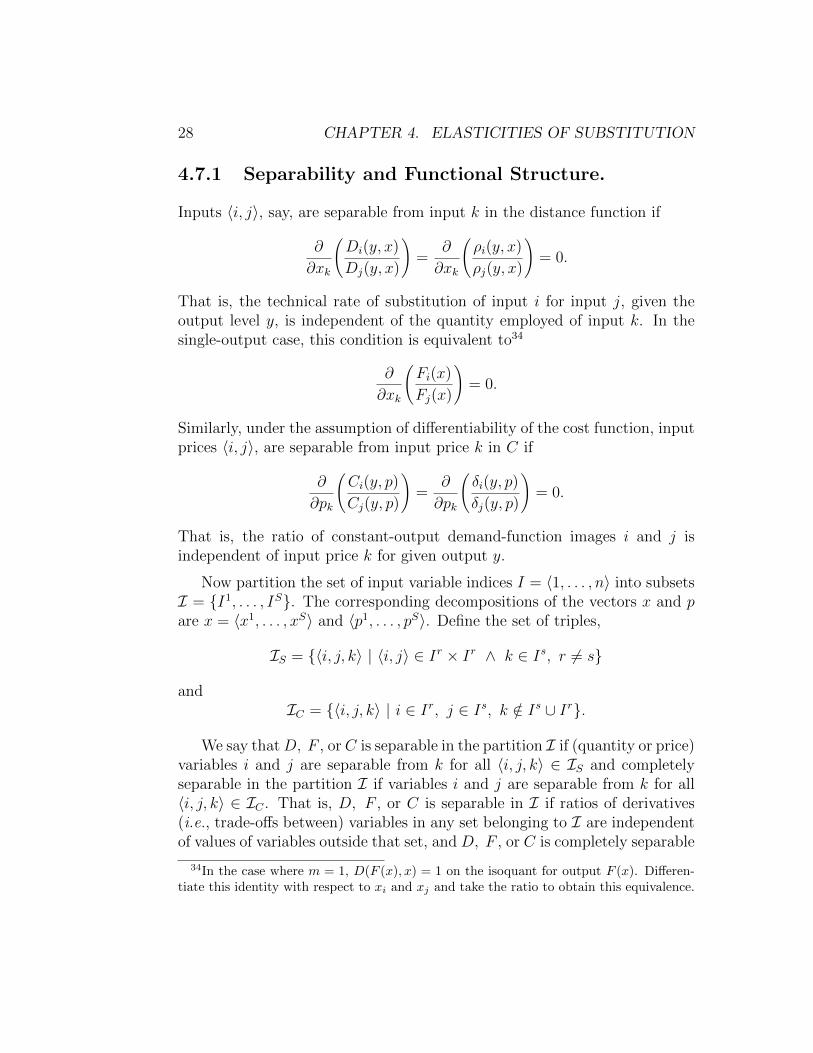
4.7.1 Separability and Functional Structure.

Inputs 〈i, j〉, say, are separable from input k in the distance function if

∂

∂xk

(Di(y, x)

Dj(y, x)

)=

∂

∂xk

(ρi(y, x)

ρj(y, x)

)= 0.

That is, the technical rate of substitution of input i for input j, given theoutput level y, is independent of the quantity employed of input k. In thesingle-output case, this condition is equivalent to34

∂

∂xk

(Fi(x)

Fj(x)

)= 0.

Similarly, under the assumption of differentiability of the cost function, inputprices 〈i, j〉, are separable from input price k in C if

∂

∂pk

(Ci(y, p)

Cj(y, p)

)=

∂

∂pk

(δi(y, p)

δj(y, p)

)= 0.

That is, the ratio of constant-output demand-function images i and j isindependent of input price k for given output y.

Now partition the set of input variable indices I = 〈1, . . . , n〉 into subsetsI = {I1, . . . , IS}. The corresponding decompositions of the vectors x and pare x = 〈x1, . . . , xS〉 and 〈p1, . . . , pS〉. Define the set of triples,

IS = {〈i, j, k〉 | 〈i, j〉 ∈ Ir × Ir ∧ k ∈ Is, r 6= s}

andIC = {〈i, j, k〉 | i ∈ Ir, j ∈ Is, k /∈ Is ∪ Ir}.

We say thatD, F , or C is separable in the partition I if (quantity or price)variables i and j are separable from k for all 〈i, j, k〉 ∈ IS and completelyseparable in the partition I if variables i and j are separable from k for all〈i, j, k〉 ∈ IC . That is, D, F , or C is separable in I if ratios of derivatives(i.e., trade-offs between) variables in any set belonging to I are independentof values of variables outside that set, and D, F , or C is completely separable

34In the case where m = 1, D(F (x), x) = 1 on the isoquant for output F (x). Differen-tiate this identity with respect to xi and xj and take the ratio to obtain this equivalence.


in I if ratios of derivatives between any two variables in I are independentof values of variables outside the sets containing the variables in the ratio.

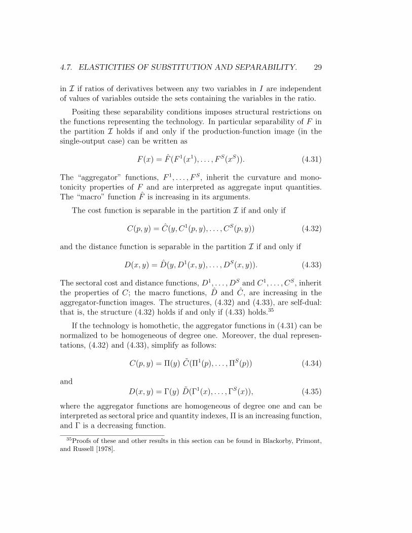
Positing these separability conditions imposes structural restrictions onthe functions representing the technology. In particular separability of F inthe partition I holds if and only if the production-function image (in thesingle-output case) can be written as

F (x) = F (F 1(x1), . . . , F S(xS)). (4.31)

The “aggregator” functions, F 1, . . . , F S, inherit the curvature and mono-tonicity properties of F and are interpreted as aggregate input quantities.The “macro” function F is increasing in its arguments.

The cost function is separable in the partition I if and only if

C(p, y) = C(y, C1(p, y), . . . , CS(p, y)) (4.32)

and the distance function is separable in the partition I if and only if

D(x, y) = D(y,D1(x, y), . . . , DS(x, y)). (4.33)

The sectoral cost and distance functions, D1, . . . , DS and C1, . . . , CS, inheritthe properties of C; the macro functions, D and C, are increasing in theaggregator-function images. The structures, (4.32) and (4.33), are self-dual:that is, the structure (4.32) holds if and only if (4.33) holds.35

If the technology is homothetic, the aggregator functions in (4.31) can benormalized to be homogeneous of degree one. Moreover, the dual represen-tations, (4.32) and (4.33), simplify as follows:

C(p, y) = Π(y) C(Π1(p), . . . ,ΠS(p)) (4.34)

and

D(x, y) = Γ(y) D(Γ1(x), . . . ,ΓS(x)), (4.35)

where the aggregator functions are homogeneous of degree one and can beinterpreted as sectoral price and quantity indexes, Π is an increasing function,and Γ is a decreasing function.

35Proofs of these and other results in this section can be found in Blackorby, Primont,and Russell [1978].


Finally, if the production function satisfies first-degree homogeneity, (4.34)and (4.35) simplify to

C(p, y) = y C(Π1(p), . . . ,ΠS(p)) (4.36)

andD(x, y) = y−1D(Γ1(x), . . . ,ΓS(x)). (4.37)

Note that, on the frontier, D(x, y) = 1 and inversion of (4.37) in y yields theproduction function (4.31).

We say that D, F , or C is completely separable in the partition I if(quantity or price) variables i and j are separable from k for all 〈i, j, k〉 ∈ ICand completely separable in the partition I if variables i and j are separablefrom k for all 〈i, j, k〉 ∈ IC .

Assume that the partition of the price and quantity variables I containsmore than two groups (S > 2).36 Then the (symmetrically dual) cost and dis-tance functions have the following images if and only if they satisfy completeseparability in the partition I:37

C(p, y) = C

(y,

S∑s=1

Cs(ps, y)

)(4.38)

= Γ(y) C

(y,

S∑s=1

Cs(ps, y)ρ(y))1/ρ(y)

, 0 6= ρ(y) ≤ 1, (4.39)

or

Γ(y)S∏s=1

Cs(ps, y)βs(y), β(y) > 0 ∀ s,

S∑s=1

βs(y) = 1, (4.40)

and

D(x, y) = D

(y,

S∑s=1

Γs(xs, y)

)(4.41)

36Don’t ask. Or if you can’t resist, I refer you to Section 4.6 of Blackorby, Primont, andRussell [1978] on “Sono independence” and additivity in a binary partition.

37Analogously to the case (4.11), ρ(y) = ρ(y)/(ρ(y)− 1

).


= Γ(y)−1 D

(y,

S∑s=1

Γs(xs, y)ρ(y))1/ρ(y)

, 0 6= ρ(y) ≤ 1, (4.42)

or

Γ(y)−1S∏s=1

Γs(xs, y)βs(y) βs(y) > 0 ∀ s,

S∑s=1

βs(y) = 1. (4.43)

Thus, complete separability results in a dual structure for the cost and dis-tance functions that is CES in the aggregator-function images, C1(p1, y), . . . ,CS(pS, y) and D1(x1, y), . . . , DS(pS, y). These aggregator function imagescannot be interpreted, however, as sectoral price and quantity indexes, sincethey depend on the value of the output vector as well as input-specific pricesand quantities. If, however, we conjoin complete separability and the as-sumption of homotheticity of the technology, the above structure simplifiesto

C(p, y) = Γ(y)

(S∑s=1

Πs(ps)ρ)1/ρ

, 0 6= ρ ≤ 1, (4.44)

or

Γ(y)S∏s=1

Πs(ps)βs , βs > 0 ∀ s,

S∑s=1

βs = 1, (4.45)

and

D(x, y) = Γ(y)−1(

S∑s=1

Λs(xs)ρ)1/ρ

, 0 6= ρ ≤ 1, (4.46)

or

Γ(y)−1S∏s=1

Λs(xs)βs , βs > 0 ∀ s,

S∑s=1

βs = 1. (4.47)

The functions, Πs(ps) and Γs(xs), s = 1, . . . , S, satisfy the salient (mono-tonicity and homogeneity) properties of price and quantity indexes, respec-tively.


If S = 1 in (4.46) and (4.47), inversion of D(x, y) = 1 yields the produc-tion function,

y = F (x) = Γ

([S∑s=1

Λs(xs)ρ]1/ρ)

, 0 6= ρ ≤ 1,

or

Γ

(S∏s=1

Λs(xs)βs), βs > 0 ∀ s,

S∑s=1

βs = 1.

If, in addition, the production function is homogeneous of degree one, Γ(y) =y and

F (x) =

[S∑s=1

Λs(xs)ρ]1/ρ

, 0 6= ρ ≤ 1,

orS∏s=1

Λs(xs)βs , βs > 0 ∀ s,

S∑s=1

βs = 1.

4.7.2 Elasticity Identities and Functional Structure.

Berndt and Christensen [1973] were the first to notice a relationship betweenfunctional structure and certain restrictions on the values of (Allen) elas-ticities of substitution. Maintaining linear homogeneity of a single-outputproduction function and n > 2, they showed that

σDMki (p, y) = σDMkj (p, y) ∀〈i, j, k〉 ∈ IS

if and only if F is separable in the partition I. This result was generalizedby Diewert [1974], Russell [1975], and Blackorby and Russell [1976], andthe latter results were extended to Morishima elasticities by Blackorby andRussell [1981]. These results can be summarized as follows:

The following conditions are equivalent (under the maintained assumptionthat n > 2):

4.8. CONCLUDING REMARKS. 33

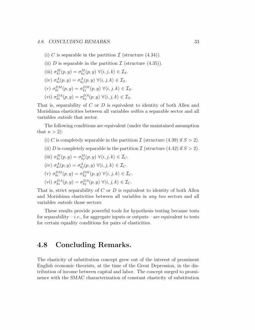
(i) C is separable in the partition I (structure (4.34)).

(ii) D is separable in the partition I (structure (4.35)).

(iii) σMki (p, y) = σMkj (p, y) ∀〈i, j, k〉 ∈ IS.(iv) σAki(p, y) = σAkj(p, y) ∀〈i, j, k〉 ∈ IS.(v) σDMki (p, y) = σDMkj (p, y) ∀〈i, j, k〉 ∈ IS.(vi) σDAki (p, y) = σDAkj (p, y) ∀〈i, j, k〉 ∈ IS.

That is, separability of C or D is equivalent to identity of both Allen andMorishima elasticities between all variables within a separable sector and allvariables outside that sector.

The following conditions are equivalent (under the maintained assumptionthat n > 2):

(i) C is completely separable in the partition I (structure (4.39) if S > 2).

(ii)D is completely separable in the partition I (structure (4.42) if S > 2).

(iii) σMki (p, y) = σMkj (p, y) ∀〈i, j, k〉 ∈ IC .(iv) σAki(p, y) = σAkj(p, y) ∀〈i, j, k〉 ∈ IC .(v) σDMki (p, y) = σDMkj (p, y) ∀〈i, j, k〉 ∈ IC .(vi) σDAki (p, y) = σDAkj (p, y) ∀〈i, j, k〉 ∈ IC .

That is, strict separability of C or D is equivalent to identity of both Allenand Morishima elasticities between all variables in any two sectors and allvariables outside those sectors.

These results provide powerful tools for hypothesis testing because testsfor separability—i.e., for aggregate inputs or outputs—are equivalent to testsfor certain equality conditions for pairs of elasticities.

4.8 Concluding Remarks.

The elasticity of substitution concept grew out of the interest of prominentEnglish economic theorists, at the time of the Great Depression, in the dis-tribution of income between capital and labor. The concept surged to promi-nence with the SMAC characterization of constant elasticity of substitution


production functions and the emergence of modern growth theory in the1960s. The elasticity of substitution between labor and capital turns out tobe fundamental to many theoretical aspects of economic growth, includingthe possibility of perpetual growth or decline, the growth of per capita in-come, the speed of convergence to an equilibrium growth path. The elasticityof substitution is especially salient in the insightful analysis of the growthprocess by Klump and de la Grandville [2000]. See Chirinko [2008] for adiscussion of these issues and references to the relevant literature.

Much of the earlier growth theory featured the Cobb-Douglas productionfunction, but particularly as accumulating empirical evidence has indicatedthat the (aggregate) elasticity of substitution is significantly less than one(see Chirinko [2008]), the CES has gained prominence. Although the CEShas only one more parameter than the Cobb-Douglas, its greater flexibilityseems to be seems to be more attuned to the evidence.

The focus of the foregoing exposition has been on the elasticity of sub-stitution between (or among) inputs, but the concept is equally relevant tooutput substitution. That is, for each of the elasticities defined above, one canformulate a corresponding (primal or dual) output elasticity of substitution—a characterization of the curvature of the output possibility curve (or sur-face).38

The elasticity of substitution also shows up in utility theory, where itreflects the ease of substitution between consumer goods (and characterizesthe curvature of indifference surfaces). The CES function made its first ap-pearance in utility theory when Burk (Bergson) [1936] showed that additivityof the utility function and linearity of Engel curves implies that the utilityfunction belongs to the CES family, referred to as the “Bergson family” inconsumer theory. The elasticity of substitution in intertemporal utility func-tions plays an important role in macroeconomic theory (Hall [1988] and inoptimal growth theory (Cass [1965], and Koopmans [1965]). Finally, the CESutility function has proved useful in the study of optimal product diversityin the context of monopolistic competition (Dixit and Stiglitz [1977]).

Consistently with the theme of this volume, the chapter has focused pri-marily on the theoretical development of the measurement of subsitutability:primal and dual characterizations and their close relationships to separable

38See, e.g., the analysis of the substitutability between a “good” and a “bad” output(in this case, electricity and sulphur dioxide) in Fare, Grosskopf, Noh, and Weber [2005].


sectors of a production or utility function. The taxonomy for n-variable elas-ticities implicit in the discussions in Sections 4.4—4.5 and 4.6 dichotomizeselasticity-of-substitution concepts along the following lines: partial vs. ra-tio elasticities (Allen vs. Morishima elasticities), direct vs. dual elasticities(quantities vs. (shadow) prices as “endogenous” variables), and net vs. grosselasticities (fixed output [or technological homotheticity] vs. variable out-put). Other elasticity-of-substitution concepts have been proposed, but I seethem as variations on these themes.39

References.Allen, R. G. D. [1938], Mathematical Analysis for Economists, London:

Macmillan.

Allen, R. G. D., and J. R. Hicks [1934], “A Reconsideration of the Theory ofValue, II,” Economica 1, N.S. 196–219.

Arrow, K. J., H. P. Chenery, B. S. Minhaus, and R. M. Solow (SMAC)[1961], “Capital-Labor Substitution and Economic Efficiency,” Review ofEconomics and Statistics 63: 225–250.

Berndt, E. R., and L. Christensen [1973], “The Internal Structure of Func-tional Relationships: Separability, Substitution, and Aggregation,” Reviewof Economic Studies 40: 403–410.

Bertoletti, P. [2001], “The Allen/Uzawa Elasticity of Substitution as a Mea-sure of Gross Input Substitutability, ” Rivista Italiana Degli Economisti6: 87–94.

Bertoletti, P. [2005], “Elasticities of Substitution and Complementarity ASynthesis,” Journal of Productivity Analysis 24:183–196.

Blackorby, C., and R. R. Russell [1975], “The Partial Elasticity of Substitu-tion,” Discussion Paper No. 75-1, Department of Economics, Universityof California, San Diego.

39This may be an unfair oversimplification: Stern [2011], building on Mundlak [1968],proposes a related but somewhat different and more comprehensive taxonomy of the elas-ticities. (Nevertheless, I’m reminded of a (private) comment made by a well-known socialchoice theorist back in the heyday of research in his area: “The problem with social choicetheory is that there are more axioms than there are ideas.” Well, maybe at some pointwe reached the point where there are more elasticity-of-substitution concepts than thereare ideas.)


Blackorby, C., and R. R. Russell [1976], “Functional Structure and the AllenPartial Elasticities of Substitution: An Application of Duality Theory,”Review of Economic Studies 43: 285–292.

Blackorby, C., and R. R. Russell [1981], “The Morishima Elasticity of Sub-stitution: Symmetry, Constancy, Separability, and Its Relationship to theHicks and Allen Elasticities,” Review of Economic Studies 48: 147–158.

Blackorby, C., and R. R. Russell [1989], “Will the Real Elasticity of Substitu-tion Please Stand Up? A Comparison of the Allen/Uzawa and MorishimaElasticities,” American Economic Review 79: 882–888.

Blackorby, C., D/ Primont, and R. R. Russell [1978], Duality, Separability,and Functional Structure: Theory and Economic Applications, New York:North-Holland.

Blackorby, C., D/ Primont, and R. R. Russell [2007], “The Morishima GrossElasticity of Substitution,” Journal of Productivity Analysis 28: 203–208.

Burk (Bergson), A. [1936], “Real Income, Expenditure Proportionality, andFrisch’s ‘New Methods of Measuring Marginal Utility’,” Review of Eco-nomic Studies 4: 33–52.

Cass, D. [1965], “Optimum Growth in an Aggregative Model of Capital Ac-cumulation,” Review of Economic Studies 32: 233–240.

Chambers, R. [1988], Applied Production Analysis, Cambridge UniversityPress, Cambridge.

Chirinko, R. S. [2008], “σ: the Long and Short of It,” Journal of Macroeco-nomics 30: 671–686.

Cobb, C. W., and P. H. Douglas [1928], “A Theory of Production,” AmericanEconomic Review 18: 23–34.

Cornes, R. [1992], Duality and Modern Economics, Cambridge: CambridgeUniversity Press.

Davis G.C, and C. R. Shumway [1996], “To Tell the Truth about Interpretingthe Morishima Elasticity of Substitution,” Canadian Journal of Agricul-tural Economics 44: 173–182.

de la Grandville, O. [1997], “Curvature and the Elasticity of Substitution:Straightening It Out,” Journal of Economics 66: 23–34.


Diewert, W. E. [1974], “Applications of Duality Theory,” in Frontiers ofQuantitative Economics , Vol. 2, edited by M. Intriligator and D. Kendrick,Amsterdam: North-Holland.

Diewert, W. E. [1982], “Duality Approaches to Microeconomic Theory,” inHandbook of Mathematical Economics, Vol. II, edited by K. Arrow andM. Intriligator, New York: North-Holland.

Dixit, A. K., and J. E. Stiglitz [1977], “Monopolistic Competition and Opti-mum Product Diversity,” American Economic Review 67: 297–308.

Fare, R., S. Grosskopf, D-W Noh, and W. Weber (2005), “Characteristics ofa Polluting Technology: Theory and Practice,” Journal of Econometrics126: 469–492.

Fare, R., and D. Primont [1995], Multi-Output Production and Duality The-ory: Theory and Applications, Boston: Kluwer Academic Press.

Fuss, M., and D. McFadden (eds.) [1978], Production Economics; A DualApproach to Theory and Applications , Amsterdam: North-Holland.

Hall, R. E. [1988], “Intertemporal Substitution in Consumption,” Journal ofPolitical Economy 96: 339–357.

Hardy, G. H., J. E. Littlewood, and G. Polya [1934], Inequalities, CambridgeUniversity Press, Cambridge.

Hicks, J. R. [1932], The Theory of Wages, MacMillan Press.

Hicks, J. R. [1970], “Elasticity of Substitution Again: Substitutes and Com-plements,” Oxford Economic Papers 22: 289–296.

Hicks, J. R., and R. G. D. Allen [1934], “A Reconsideration of the Theory ofValue, Part II,” Economica 1, N.S. 196–219.

Houthakker, H,. S [1965], “A Note on Self-Dual Preferences,” Econometrica33: 797–801.

Kim, H. Y. [2000], “The Antonelli versus Hicks Elasticity of Complementarityand Inverse Input Demand Systems,” Australian Economic Papers 39: 245-261.

Klump, R., and O. de la Grandville [2000], “Economic Growth and the Elas-ticity of Substitution: Two Theorems and Some Suggestions, AmericanEconomic Review 90:282–291.


Koopmans, T. C. [1965], “On the Concept of Optimal Economic Growth,”in The Economic Approach to Development Planning, Chicago: RandMcNally.

Kuga, K. [1979], On the Symmetry of Robinson Elasticities of Substitution:the General Case” Review of Economic Studies 46: 527–531.

Kuga, K., and T. Murota [1972], “A Note on Definition of Elasticity ofSubstitution,” Macroeconomica 24: 285–290.

Lau, L. [1978], “Applications of Profit Functions,” in M. Fuss and D. Mc-Fadden (eds.), Production Economics: A Dual Approach to Theory andApplications, Amsterdam: North-Holland, 133–216.

Leontief, W. W. [1953], “Domestic Production and Foreign Trade: TheAmerican Capital Position Re-examined,” Proceedings of the AmericanPhilosophical Society 97: 331–349.

Leontief, W. W. [1947a], “A Note on the Interrelation of Subsets of Indepen-dent Variables of a Continuous Function with Continuous First Deriva-tives,” Bulletin of the American Mathematical Society 53: 343–350.

Leontief, W. W. [1947b], “Introduction to a Theory of the Internal Structureof Functional Relationships,” sl Econometrica 15: 361–373.

Lerner A.P. [1933], “Notes on the Elasticity of Substitution II: the Diagram-matical Representation,” Review of Economic Studies 1: 68–70.

McFadden, D. [1963], “Constant Elasticity of Substitution Production Func-tions,” Review of Economic Studies 30: 73–83.

Morishima, M. [1967], “A Few Suggestions on the Theory of Elasticity” (inJapanese), Keizai Hyoron (Economic Review) 16: 144–150.

Mundlak, Y. [1968], “Elasticities of Substitution and the Theory of DerivedDemand,” Review of Economic Studies 35: 225–236.

Murota, T. [1977], “On the Symmetry of Robinson Elasticities of Substitu-tion: A Three-Factor Case,” Review of Economic Studies 42:79–85.

Pigou A.C. [1934], “The Elasticity of Substitution,” Economic Journal 44:23–241.

Robinson, J. [1933], Economics of Imperfect Competition, London: MacMil-lan.


Russell, R. R. [1976], “Functional Separability and Partial Elasticities ofSubstitution,” Review of Economic Studies 42: 79–85.

Russell, R. R. [1997], “Distance Functions in Consumer and Producer The-ory,” Essay 1 in Index Number Theory: Essays in Honor of Sten Malmquist,Boston: Kluwer Academic Publishers, 7–90 .

Sato, R., and T. Koizumi [1973], “On the Elasticities of Substitution andComplementarity,” Oxford Economic Papers 25: 44–56.

Solow, R. M. [1956], “A Contribution to the Theory of Economic Growth,”Quarterly Journal of Economics 65: 65–94.

Sono, M. [1961], “The Effect of Price Changes on the Demand and Supplyof Separable Goods,” International Economic Review 2: 239–271.

Stern, D. I. [2010], “Derivation of the Hicks, or Direct, Elasticity of Substitu-tion from the Input Distance Function,” Economic Letters 108: 349–351.

Stern D. I. [2011], “Elasticities of Substitution and Complementarity,” Jour-nal of Productivity Analysis 36: 79-89.

Syrquin, M, and G. Hollender [1982], “Elasticities of Substitution and Com-plementarity: the General Case,” Oxford Economic Papers 34: 515–519.

Uzawa, H. [1962], “Production Functions with Constant Elasticities of Sub-stitution,” Review of Economic Studies 29: 291–299.

elasticities of substitution - economics:...

Documents