Elasticities and theInverse Hyperbolic Sine Transformation∗

Marc F. Bellemare†

Casey J. Wichman‡

February 24, 2019

Abstract

Applied econometricians frequently apply the inverse hyperbolicsine (or arcsinh) transformation to a variable because it approximatesthe natural logarithm of that variable and allows retaining zero-valuedobservations. We provide derivations of elasticities in common appli-cations of the inverse hyperbolic sine transformation and show empir-ically that the difference in elasticities driven by ad hoc transforma-tions can be substantial. We conclude by offering practical guidancefor applied researchers.

Keywords: Elasticities, Elasticity, Inverse Hyperbolic Sine, arcsinhJEL Classification Codes: C1, C5Word Count: 4,279

∗We are grateful to James Fenske and three anonymous reviewers for their commentsand suggestions. We also thank Jeff Bloem, Dave Giles, Seema Jayachandran, JasonKerwin, David McKenzie, Steve Miller, and Joseph Ritter for comments on an earlierversion of this paper. All remaining errors are ours.†Northrop Professor, Department of Applied Economics, University of Minnesota, 1994

Buford Avenue, Saint Paul, MN 55108, mbellema@umn.edu‡Fellow, Resources for the Future, 1616 P Street NW, Suite 600, Washington, DC

20036, wichman@rff.org.

1

ELASTICITIES AND THE INVERSE HYPERBOLIC SINETRANSFORMATION

Abstract

Applied econometricians frequently apply the inverse hyperbolicsine (or arcsinh) transformation to a variable because it approximatesthe natural logarithm of that variable and allows retaining zero-valuedobservations. We provide derivations of elasticities in common appli-cations of the inverse hyperbolic sine transformation and show empir-ically that the difference in elasticities driven by ad hoc transforma-tions can be substantial. We conclude by offering practical guidancefor applied researchers.

Keywords: Elasticities, Elasticity, Inverse Hyperbolic Sine, arcsinhJEL Classification Codes: C1, C5Word Count: 4,279

2

1 Introduction

Applied econometricians often transform variables to make the interpretation

of empirical results easier, to approximate a normal distribution, to reduce

heteroskedasticity, or to reduce the effect of outliers. Taking the logarithm

of a variable has long been a popular such transformation.

One problem with taking the logarithm of a variable is that it does not

allow retaining zero-valued observations because ln(0) is undefined. But eco-

nomic data often include meaningful zero-valued observations, and applied

econometricians are typically loath to drop those observations for which the

logarithm is undefined. Consequently, researchers have often resorted to ad

hoc means of accounting for this when taking the natural logarithm of a vari-

able, such as adding 1 to the variable prior to its transformation (MaCurdy

and Pencavel, 1986).

In recent years, the inverse hyperbolic sine (or arcsinh) transformation has

grown in popularity among applied econometricians because (i) it is similar

to a logarithm, and (ii) it allows retaining zero-valued (and even negative-

valued) observations (Burbidge et al., 1988; MacKinnon and Magee, 1990;

Pence, 2006).1

For a random variable x, taking the inverse hyperbolic sine transformation

1As Ravallion (forthcoming) notes, in cases where a concave log-like transformationof negative data is necessary, the inverse hyperbolic sine transformation has undesirableproperties, viz. it is convex over negative values. Given that, and because the inversehyperbolic sine transformation is largely used with nonnegative variables (e.g., earnings),we focus in this paper only on cases where the variable to which the inverse hyperbolicsine transformation is applied is nonnegative.

3

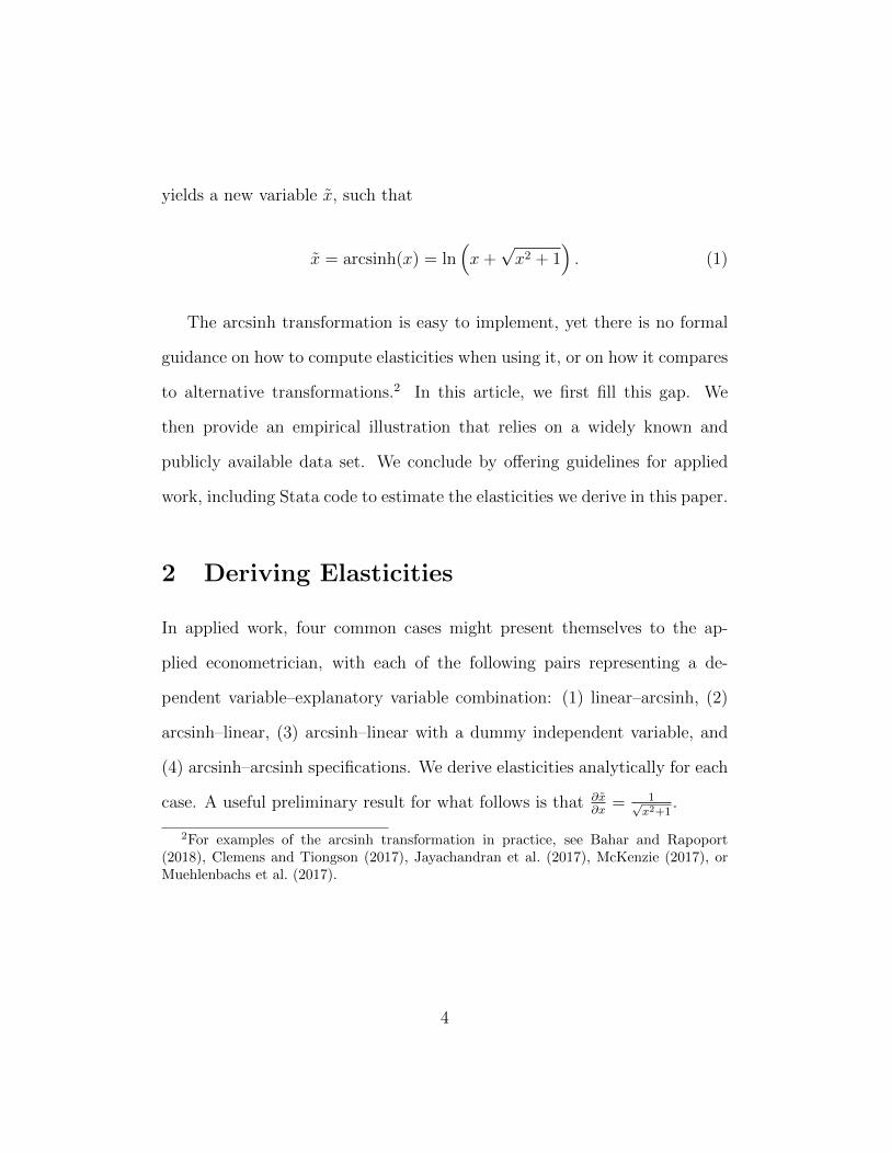
yields a new variable x, such that

x = arcsinh(x) = ln(x+√x2 + 1

). (1)

The arcsinh transformation is easy to implement, yet there is no formal

guidance on how to compute elasticities when using it, or on how it compares

to alternative transformations.2 In this article, we first fill this gap. We

then provide an empirical illustration that relies on a widely known and

publicly available data set. We conclude by offering guidelines for applied

work, including Stata code to estimate the elasticities we derive in this paper.

2 Deriving Elasticities

In applied work, four common cases might present themselves to the ap-

plied econometrician, with each of the following pairs representing a de-

pendent variable–explanatory variable combination: (1) linear–arcsinh, (2)

arcsinh–linear, (3) arcsinh–linear with a dummy independent variable, and

(4) arcsinh–arcsinh specifications. We derive elasticities analytically for each

case. A useful preliminary result for what follows is that ∂x∂x

= 1√x2+1

.

2For examples of the arcsinh transformation in practice, see Bahar and Rapoport(2018), Clemens and Tiongson (2017), Jayachandran et al. (2017), McKenzie (2017), orMuehlenbachs et al. (2017).

4

2.1 Linear–arcsinh Specification

Consider the following estimable equation

y = α + βx+ ε. (2)

In this case, computing ξyx = ∂y∂x· xy

after estimating the previous equation is

relatively straightforward, since ∂y∂x

= β√x2+1

, and so

ξyx =β

y

x√x2 + 1

. (3)

Because limx→∞x√x2+1

= 1, for large values of x, ξyx ≈ βy.3

2.2 arcsinh–Linear Specification

Now, consider an estimable equation of the form

y = α + βx+ ε (4)

where x is a continuous variable. In this case, to recover y from the left-hand

side of the equation of interest after estimating the previous equation, one

has to apply the hyperbolic sine transformation—that is, the inverse of the

3We discuss what we mean by “large values of x” in sub-section 2.5.

5

inverse hyperbolic sine, or sinh—on both sides, so that

y = sinh(α + βx+ ε). (5)

In this case, to recover ξyx = ∂y∂x· xy, we need to multiply x

yby ∂y

∂x= β cosh(α+

βx+ ε) to get

ξyx = β cosh(α + βx+ ε) · xy, (6)

which can be rewritten as

ξyx = β cosh(arcsinh(y)) · xy

= βx ·√y2 + 1

y. (7)

In this case, because limy→∞

√y2+1

y= 1, for large values of y, ξyx ≈ βx.

2.3 arcsinh–Linear Specification with Dummy Inde-

pendent Variables

Dummy variables pose a different set of problems for calculating elasticities,

and this problem is not unique to arcsinh–linear econometric specifications.

Standard log-linear specifications also suffer from this problem (Halvorsen

and Palmquist, 1980; Kennedy, 1981). Consider the estimable equation

y = α + βd+ ε (8)

6

where d is a dichotomous variable taking on only values of zero or one.

The quantity ∂y/∂d is undefined because dichotomous variables only change

discretely. Following the arguments of Halvorsen and Palmquist (1980),

Kennedy (1981), and Giles (1982) for semilogarithmic regression equations

with dummy variables, we derive the analogous proportional effect for the

arcsinh transformation, which we denote P .

To derive P , the percentage change in y associated with a change from

d = 0 to d = 1, we first apply the sinh transformation to both sides, such

that

sinh(y) = y = sinh(α + βd+ ε). (9)

After estimating Eq. 8, P is then defined as

ˆP

100=y(d = 1)− y(d = 0)

y(d = 0)=

sinh(α + β + ε)− sinh(α + ε)

sinh(α + ε)

=sinh(α + β + ε)

sinh(α + ε)− 1

(10)

Researchers often adopt the arcsinh transformation to approximate a log-

arithm and interpret coefficients as they would for a logarithmic equation. In

this case, one can approximate semi-elasticities as shown by Halvorsen and

Palmquist (1980), Kennedy (1981), and Giles (1982) by exponentiating both

sides of Eq. 8 and noting that

exp(y) = y +√y2 + 1 ≈ 2y for large y.

7

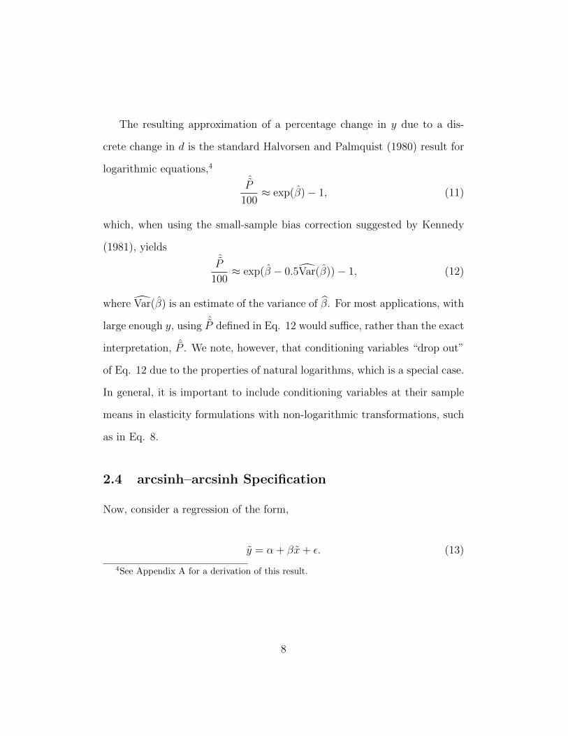
The resulting approximation of a percentage change in y due to a dis-

crete change in d is the standard Halvorsen and Palmquist (1980) result for

logarithmic equations,4

ˆP

100≈ exp(β)− 1, (11)

which, when using the small-sample bias correction suggested by Kennedy

(1981), yieldsˆP

100≈ exp(β − 0.5Var(β))− 1, (12)

where Var(β) is an estimate of the variance of β. For most applications, with

large enough y, using ˆP defined in Eq. 12 would suffice, rather than the exact

interpretation, ˆP . We note, however, that conditioning variables “drop out”

of Eq. 12 due to the properties of natural logarithms, which is a special case.

In general, it is important to include conditioning variables at their sample

means in elasticity formulations with non-logarithmic transformations, such

as in Eq. 8.

2.4 arcsinh–arcsinh Specification

Now, consider a regression of the form,

y = α + βx+ ε. (13)

4See Appendix A for a derivation of this result.

8

In this last case, in order to recover y from the left-hand side of the equa-

tion of interest after estimating the previous equation, one has to apply the

hyperbolic sine transformation on both sides, so that

y = sinh(α + βx+ ε). (14)

In this case, ∂y∂x

= β cosh(α+βarcsinh(x)+ε)√x2+1

, so that

ξyx =β cosh(α + βarcsinh(x) + ε)√

x2 + 1· xy

. (15)

Because the argument of the cosh function is equal to y, we can rewrite this

last equation as

ξyx =β cosh(arcsinh(y))√

x2 + 1· xy

= β ·√y2 + 1

y· x√

x2 + 1. (16)

Because limx→∞x√x2+1

= 1 and limy→∞

√y2+1

y= 1, for large values of x and

y, ξyx ≈ β.

2.5 Caveats

In the literature, the elasticities just derived are interpreted as the elasticities

one would obtain from equivalent specifications with logarithmic transforma-

tions, but this only holds for large enough average values of x, y, or both.

This begs the question of how large is large enough. We suggest applied

9

econometricians use approximate elasticities for values of x or y no less than

10. Although this value seems arbitrary, we suggest it because values greater

than 10 reduce approximation error to less than half of a percent. Obviously,

greater thresholds will yield greater accuracy.

Indeed, starting from the equation y = α + βx + ε, wherein ξyx = βxy

,

multiplying y by k > 0 will return a coefficient on x equal to βk, and the

elasticity ξyx will be such that ∂y∂x· xy

= βkxyk

, so that ξyx = βxy

. Likewise, mul-

tiplying x by k will change the coefficient but leave the elasticity unaffected.

In this linear–linear case, rescaling y or x does not change the elasticity.

When an arcsinh transformation is involved, however, Monte Carlo sim-

ulations show that ξyx becomes more stable k increases. Specifically, we

have generated a data set containing 1, 000 observations on three variables:

x ∼ N(10, 2), e ∼ N(0, 2), and y, which is such that

ky = 5 + 0.5kx+ e (17)

The results of those simulations are shown for values of k equal to 1, 5, 10,

50, 100, 1,000, and 10,000 respectively for the linear–linear, linear–arcsinh,

arcsinh–linear, and arcsinh–arcsinh cases in Table 1. As k gets larger, the

elasticities rapidly become more stable. For k > 10, there is virtually no

discernable change in the elasticity estimates as k increases.

Lastly, recall that applied econometricians often adopt the arcsinh trans-

formation to deal with variables with zero-valued observations, and the pres-

10

ence of such observations at low (i.e., zero) values of x or y may result in

biased elasticity estimates. In these cases, researchers should calculate elas-

ticities using their exact formulations derived in equations 3, 7, and 16. But

because all three elasticities are undefined when y = 0, we suggest the fol-

lowing. Defining y = 1N

∑Ni=1 yi, one workaround when y = 0 is to multiply

by xy

instead of by xy, i.e., to report the elasticity at the means of x and y

instead of one of the mean elasticities we derive above.

3 Empirical illustration

We illustrate common uses of the inverse-hyperbolic sine transformation us-

ing data from Dehejia and Wahba (1999), who evaluated LaLonde’s (1986)

canonical design-replication experiment for the National Supported Work

(NSW) demonstration.

In that experiment, disadvantaged workers were randomly assigned either

to the NSW program, wherein they were given counseling and work experi-

ence, or to the control group, wherein they received neither of those things.

We use the Dehejia and Wahba (1999) subset of LaLonde’s (1986) original

data.

The outcome of interest is post-treatment annual earnings, Earnings78.

Because this application is for illustrative purposes, we focus on estimating

the treatment effect of the NSW program controlling for pre-treatment earn-

ings only. The inverse hyperbolic sine transformation of earnings is poten-

11

tially attractive because earnings data tends to be right-skewed and there is a

nontrivial number of true zeros in the data. As shown in Table 1, Earnings78

has 45 and 92 zero-valued observations respectively for the treatment and

control groups, with 111 and 178 zero-valued pre-treatment earnings obser-

vations respectively for the treatment and control groups.

We estimate four simple specifications that capture each of the cases de-

scribed above, as well as two models with the oft-used ln(x+1) transformation

for comparison. Results are presented in Table 2.5

In column (1), we see that the NSW job-training program increased post-

treatment earnings of the treated group by $1,750 per year relative to the

control group. This estimate is illustrative of the estimate in Dehejia and

Wahba (1999) Table 3, panel B, row 1. We calculate a semi-elasticity by

dividing the treatment coefficient by the sample mean of the dependent vari-

able to show that NSW increased earnings of treated individuals by approxi-

mately 33%. We also calculate the earnings elasticity between pre- and post-

treatment earnings, which shows that as pre-treatment earnings increase by

10%, we observe a 4.3% increase in post-treatment earnings. This elasticity

does not have a meaningful economic interpretation, although it is useful for

comparing elasticity calculations.

In column (2), we transform pre-treatment earnings using the arcsinh

5Before interpreting our results, we reiterate that this empirical exercise is intended toillustrate how ad hoc transformations can lead to changes in elasticity interpretations. Weinclude several goodness-of-fit statistics for the interested reader, although choosing thespecification that fits best is not the purpose of the illustration.

12

transformation. This adjustment reduces the earnings elasticity from 0.043 to

0.026, a nearly 40 percent reduction. This is a drastic change for a seemingly

innocuous transformation of an independent variable, likely due to having

reduced the influence of outliers (e.g., very high earners on average) as a

result of the inverse hyperbolic sine transformation. The coefficient on NSW,

however, remains stable, suggesting that the arcsinh transformation of a

control variable does not affect causal interpretation of treatment variables

and can improve the fit of the model.

In columns (3) and (4), we repeat this analysis for arcsinh transformation

of an independent variable: post-treatment earnings. Here, we see notable

deviations from the linear–arcsinh case. Focusing on the earnings elasticity,

we find a similar pattern as in columns (1) and (2): applying the arcsinh

transformation to post-treatment earnings reduces the elasticity estimate by

a factor of two. These elasticities, overall, are substantially larger than that

of the linear case. This illustration shows that a transformation of the de-

pendent variable can have a drastic effect on elasticity estimates.

We also present in columns (3) and (4) semi-elasticity estimates of NSW

on earnings calculated both by exact methods (P ) and by the logarithmic ap-

proximation (P ). Results suggest that NSW increased earnings by 158–188

percent. These results highlight the danger of interpreting coefficient esti-

mates directly as semi-elasticities for large coefficients on dummy variables

in arcsinh–linear regression equations. In both columns, P is approximately

25 percentage points larger than P . This difference stems almost entirely

13

from the small-sample adjustment in P . Because earnings are large in our

application, the difference in P and P before the small-sample adjustment is

trivial, suggesting the simpler logarithmic approximation performs well.

Finally, in columns (5) and (6), we repeat the previous analysis but substi-

tute the ln(x+ 1) transformation for the arcsinh transformation. Our results

for ξ(Earnings78,Earnings75) are largely analogous to the arcsinh case. This

similarity suggests that common transformations of dependent and indepen-

dent variables with a large proportion of zeros and outliers can have substan-

tial implications for elasticity estimates. For semi-elasticities, we find that

transforming dependent variables by logarithms produces percentage changes

about 15–20 percentage points smaller than arcsinh transformations (shown

in columns (3) and (4)) in our application.

We do not take a stand on whether the effect of the NSW program pre-

sented in this sequence of results is the true effect of job-training programs

on earnings; that is not the point of this paper. Rather, we show that under

seemingly innocuous, oft-used transformations of dependent and independent

variables, we can produce wildly different elasticity estimates even within a

randomized design. We view this simple analysis as a cautionary warning

to applied econometricians about using ad hoc transformations to deal with

zero-valued observations and to facilitate easy interpretation of empirical re-

sults.

14

4 Summary and Concluding Remarks

We have first derived exact elasticities in cases where an applied econome-

trician applies the increasingly popular inverse hyperbolic sine (or arcsinh)

transformation to a variable, characterizing elasticities for the cases where

the arcsinh transformation is applied to (i) an explanatory variable of in-

terest, (ii) the dependent variable with a continuous explanatory variable of

interest, (iii) the dependent variable with a dichotomous explanatory vari-

able of interest, and (iv) both the dependent variable and the explanatory

variable of interest.

After discussing some of the caveats of our approach, we have derived

those elasticities for a well-known application, which has provided a caution-

ary tale regarding the use of ad hoc transformations of variables when dealing

with zero-valued observations.

We conclude with the following guidelines for applied researchers who

wish to use the inverse hyperbolic sine transformation in their own work to

obtain elasticities:

1. One needs to be careful when interpreting inverse hyperbolic sine co-

efficients as semi-elasticities. In most cases, the researcher will need

to transform those coefficients in the manner derived above prior to

interpreting them as percentage changes. In our empirical example, in-

terpreting β on NSW as a semi-elasticity in an arcsinh–linear equation

understates the correct percentage effect by 40 percent.

15

2. Standard logarithmic adjustments for semi-elasticities in arcsinh–linear

equations with dummy variables can be used with little error for de-

pendent variables with untransformed means roughly greater than 10.

3. Applying the inverse hyperbolic sine transformation to an explanatory

variable of interest appears somewhat harmless, but it can change elas-

ticities relative to the linear-linear model substantially.

4. For cases where the applied researcher is dealing with data that contain

too many zero-valued observations, it is probably better to model the

data-generating process explicitly, e.g., using a Tobit or zero-inflated

Poisson or negative binomial model.6 Unfortunately, there is no way

to know what “too many” means in this context and so as a rule of

thumb, we submit that if the data has more than one third zero-valued

observations, it is perhaps best to explicitly model selection out of zero

and into the positive domain.

5. It is easy to obtain a more stable elasticity estimate by multiplying the

variable to which the arcsinh transformation is applied by a constant

k > 1. As k increases, the approximation error of the elasticity esti-

6In developing countries, for example, many agricultural producers do not use chemicalfertilizer, preferring instead to use organic fertilizer. In such cases, it is not uncommon tohave a data set where roughly half of the observations report using no chemical fertilizer,and those observations are coded as zeros. In such cases, the applied econometrician caneither explicitly model the data-generating process—say, by estimating a type II Tobitwhere the first stage looks at whether a producer uses chemical fertilizer and the secondstage looks at how much chemical fertilizer the same producer uses conditional on usingit in the first place.

16

mate is reduced. So for example, one can get more stable estimates by

taking the arcsinh of a price in dollars rather than of the same price in

thousands of dollars.

6. As with other elasticity estimates that rely on nonlinear combinations

of coefficients and data, standard errors should be obtained using the

delta method.

7. In Appendix B, we present Stata code that calculates elasticities in the

cases presented in sections 2.1 to 2.4.

Overall, the inverse hyperbolic sine function can be a useful tool for econo-

metricians using variables with extreme values and true zeros. For large

positive values, arcsinh can generally be treated like a natural logarithm.

Future research might consider small-sample adjustments in the elasticity

formulations we have presented here.

17

References

Angrist, Joshua D. and Jorn-Steffen Pischke, Mostly Harmless Econo-metrics: An Empiricist’s Companion, Princeton university press, 2008.

Bahar, Dany and Hillel Rapoport, “Migration, Knowledge Diffusion,and the Comparative Advantage of Nations,” Economic Journal, 2018,128 (July), F273–F305.

Burbidge, John B., Lonnie Magee, and A. Leslie Robb, “Alterna-tive transformations to handle extreme values of the dependent variable,”Journal of the American Statistical Association, 1988, 83 (401), 123–127.

Clemens, Michael A. and Erwin R. Tiongson, “Split Decisions: House-hold Finance When a Policy Discontinuity Allocates Overseas Work,” Re-view of Economics and Statistics, 2017, 99 (3), 531–543.

Dehejia, Rajeev H. and Sadek Wahba, “Causal effects in nonexperimen-tal studies: Reevaluating the evaluation of training programs,” Journal ofthe American Statistical Association, 1999, 94 (448), 1053–1062.

Giles, David E.A., “The interpretation of dummy variables in semilog-arithmic equations: Unbiased estimation,” Economics Letters, 1982, 1-2(10), 77–79.

Halvorsen, Robert and Raymond Palmquist, “The interpretation ofdummy variables in semilogarithmic equations,” American Economic Re-view, 1980, 70 (3), 474–75.

Jayachandran, Seema, Joost de Laat, Eric F. Lambin, Charlotte Y.Stanton, Robin Audy, and Nancy E. Thomas, “Cash for Carbon: ARandomized Trial of Payments for Ecosystem Services to Reduce Defor-estation,” Science, 2017, 21 (6348), 267–273.

Kennedy, Peter E., “Estimation with correctly interpreted dummy vari-ables in semilogarithmic equations,” American Economic Review, 1981, 71(4).

LaLonde, Robert J., “Evaluating the econometric evaluations of train-ing programs with experimental data,” American Economic Review, 1986,pp. 604–620.

18

MacKinnon, James G. and Lonnie Magee, “Transforming the depen-dent variable in regression models,” International Economic Review, 1990,pp. 315–339.

MaCurdy, Thomas E. and John H. Pencavel, “Testing between com-peting models of wage and employment determination in unionized mar-kets,” Journal of Political Economy, 1986, 94 (3, Part 2), S3–S39.

McKenzie, David, “Identifying and Spurring High-Growth Entrepreneur-ship: Experimental Evidence from a Business Plan Competition,” Ameri-can Economic Review, 2017, 107 (8), 2278–2307.

Muehlenbachs, Lucija, Stefan Staubli, and Ziyan Chu, “The Acci-dent Externality from Trucking,” Technical Report, National Bureau ofEconomic Research 2017.

Pence, Karen M., “The role of wealth transformations: An applicationto estimating the effect of tax incentives on saving,” The B.E. Journal ofEconomic Analysis & Policy, 2006, 5 (1).

Ravallion, Martin, “A Concave Log-Like Transformation Allowing Non-Positive Values,” Economics Letters, forthcoming.

19

Table 1: Simulation results for arbitrarily scaling dependent and in-dependent variables by a constant k ≥ 1

Empirical specification

Linear-linear Linear-arcsinh arcsinh-linear arcsinh-arcsinh

Values of k :1 0.476063 0.433217 0.500552 0.4603905 0.476063 0.432082 0.501383 0.46008110 0.476063 0.432046 0.501410 0.46007150 0.476063 0.432034 0.501419 0.460068100 0.476063 0.432034 0.501419 0.4600681000 0.476063 0.432033 0.501419 0.46006810,000 0.476063 0.432034 0.501419 0.460068

Notes: This table presents elasticity estimates from different empirical specifications basedon a simulated data set where x ∼ N(10, 2), e ∼ N(0, 2), and ky = 5 + 0.5kx+ e for variousvalues of k.

20

Table 2: Summary statistics of Dehejia andWahba (1999) NSW data

Treatment Group Control Group

Mean SD Mean SDEarnings78 6349.1 7867.4 4554.8 5483.8Earnings75 1532.1 3219.3 1266.9 3103.0Observations 185 260Earnings78 = 0 45 92Earnings75 = 0 111 178

Notes: This table presents summary statistics for the Dehejiaand Wahba (1999) sample of LaLonde’s (1986) original data.Only earnings data and treatment indicators are used in thisanalysis.

21

Tab

le3:

Illu

stra

tion

ofco

mm

onin

vers

e-hyp

erb

olic

sine

tran

sfor

mat

ions

and

elas

tici

ties

usi

ng

dat

afr

omD

ehej

iaan

dW

ahba

(199

9)

Earn

ings 7

8arc

sin

h(E

arn

ings 7

8)

ln(E

arn

ings 7

8+

1)

(1)

(2)

(3)

(4)

(5)

(6)

NS

W1750.2∗∗∗

1694.3∗∗∗

1.0

56∗∗

1.0

34∗∗

0.9

82∗∗

0.9

60∗∗

(632.1

)(6

33.9

)(0

.416)

(0.4

17)

(0.3

86)

(0.3

87)

Ear

nin

gs75

0.1

67∗

0.0

00112∗

0.0

00105∗

(0.0

990)

(0.0

000651)

(0.0

000604)

arcs

inh

(Ear

nin

gs75)

135.5∗

0.0

705

(76.8

6)

(0.0

506)

ln(E

arn

ings

75

+1)

0.0

722

(0.0

510)

Con

stan

t4343.6∗∗∗

4197.8∗∗∗

5.8

03∗∗∗

5.7

59∗∗∗

5.3

65∗∗∗

5.3

23∗∗∗

(426.1

)(4

54.7

)(0

.280)

(0.2

99)

(0.2

60)

(0.2

78)

Ob

s445

445

445

445

445

445

Ad

j.R

20.0

197

0.0

203

0.0

173

0.0

150

0.0

174

0.0

152

AIC

9088.6

9088.4

2567.3

2568.4

2500.7

2501.8

BIC

9100.9

9100.7

2579.6

2580.7

2513.0

2514.0

Log

-lik

elih

ood

-4541.3

-4541.2

-1280.7

-1281.2

-1247.4

-1247.9

Calculated

(semi-)elasticities:

ξ(E

arn

ings

78,

NS

W)

0.3

30

0.3

20

(0.1

19)

(0.1

20)

ξ(E

arn

ings

78,

Ear

nin

gs75)

0.0

433

0.0

256

0.1

55

0.0

705

0.1

44

0.0

722

(0.0

257)

(0.0

145)

(0.0

896)

(0.0

506)

(0.0

831)

(0.0

510)

P(E

arn

ings

78,

NS

W)/

100

1.6

38

1.5

78

1.4

77

1.4

24

(1.0

96)

(1.0

76)

(0.9

55)

(0.9

38)

P(E

arn

ings

78,

NS

W)/

100

1.8

76

1.8

13

(1.1

95)

(1.1

74)

Note

s:T

his

tab

lep

rese

nts

illu

stra

tive

regre

ssio

nre

sult

su

sin

gd

ata

from

the

evalu

ati

on

of

the

Nati

on

al

Su

pp

ort

edW

ork

exp

erim

ent

by

Deh

ejia

an

dW

ahb

a(1

999)

an

dre

pro

du

ced

inT

ab

le3.3

.3of

An

gri

stan

dP

isch

ke

(2008).

Data

are

ob

tain

edfr

om

https://economics.mit.edu/faculty/angrist/data1/mhe/dehejia

(Last

Acc

esse

d:

Ju

ne

1,

2018).

NS

Wis

ad

um

my

vari

ab

lesi

gn

ifyin

gass

ign

men

tto

the

ran

dom

ized

trea

tmen

tgro

up

.E

arn

ings 7

8an

dE

arn

ings 7

5are

an

nu

al

earn

ings

(in

dollars

)fo

r1978

an

d1975,

resp

ecti

vel

y.A

ll(s

emi-

)ela

stic

itie

sare

calc

ula

ted

at

the

sam

ple

mea

n.

22

Appendix A

Consider the modelarcsinh(y) = α + βd+ ε (A.1)

To approximate P , the percentage change in y due to a change in the dummyvariable d, we exponentiate both sides of Eq. A.1 after estimation,

exp(arcsinh(y)) = y +√

(y2 + 1) ≈ 2y = exp(α + βx+ ε) (A.2)

where the approximation holds for large y.We then define the percentage change in y due to a discrete change in d,

P

100=y(d = 1)− y(d = 0)

y(d = 0)

=12

exp(α + βx+ ε)− 12

exp(α + ε)12

exp(α + ε)= exp(β)− 1.

(A.3)

A.1

Appendix B

This section we presents Stata code to estimate the elasticities discussed inthis paper for the simple case where there are only two variables: the depen-dent variable y, and the explanatory variable of interest x. Before anythingelse, the following preliminary lines of code are necessary:

egen xbar = mean(x)

egen ybar = mean(y)

gen ihs_x = asinh(x)

gen ihs_y = asinh(y)

where xbar and ybar are respectively the means of the explanatory vari-able of interest and of the dependent variable, ihs_x denotes the inversehyperbolic sine transformation x, and ihs_y denotes the inverse hyperbolicsine transformation y.

Turning to elasticities, recall that for the standard case, the elasticity canbe estimated as follows:

reg y x

nlcom _b[x]*xbar/ybar

Similarly, for the linear-arcsinh case, the elasticity can be estimated asfollows:

reg y ihs_x

nlcom (_b[ihs_x]*xbar)/(ybar*sqrt(xbar^2+1))

Likewise, the elasticity for the arcsinh-linear case can be estimated asfollows:

reg ihs_y x

nlcom _b[x]*xbar*((sqrt(ybar^2+1))/ybar)

Finally, the elasticity for the arcsinh-arcsinh case can be estimated asfollows:

A.2

reg ihs_y ihs_x

nlcom (_b[ihs_x]*xbar*(sqrt(ybar^2+1)))/(ybar*sqrt(xbar^2+1))

In all case, Stata estimates the standard errors using the delta method.

A.3