Eindhoven University of Technology

MASTER

Elastic recoil detection analysis with He Ions : simulations and applications to materialsanalysis

Jaegers, Lucien

Award date:1994

Link to publication

DisclaimerThis document contains a student thesis (bachelor's or master's), as authored by a student at Eindhoven University of Technology. Studenttheses are made available in the TU/e repository upon obtaining the required degree. The grade received is not published on the documentas presented in the repository. The required complexity or quality of research of student theses may vary by program, and the requiredminimum study period may vary in duration.

General rightsCopyright and moral rights for the publications made accessible in the public portal are retained by the authors and/or other copyright ownersand it is a condition of accessing publications that users recognise and abide by the legal requirements associated with these rights.

• Users may download and print one copy of any publication from the public portal for the purpose of private study or research. • You may not further distribute the material or use it for any profit-making activity or commercial gain

,---------1 Lill-/ 00a

Master of Science Thesis

Elastic Recoil Detection Analysis With He Ions simulations and applications to

materials analysis

Lucien Jaegers

VDF/NK 94-15

Cyclotron Laboratory Eindhoven University of Technology P.O. box 513 5600 MB Eindhoven The Netherlands

Prof. dr. M.J.A. de Voigt Dr. L.J. van Ijzendoorn

SUMMARY

At the Eindhoven University of Technology Cyclotron Laboratory analysis of light elements in a heavy matrix, e.g. BxCyNzH or oxynitride layers on silicon, is performed. Experiments are carried out with the ion beam analysis technique Elastic Recoil Detection using a beam of high energetic (10-15 MeV) a particles (o:-ERD). Contrary to RBS, where the energy of the backscattered incident particles is measured, ERD measures the energies of ions recoiled from the target sample.

In order to significantly improve interpretation of the measured spectra software has been written which allows rigorously simulation of ERD spectra.

The most essential requirement for ERD to succeed is discrimination between the scat­tered and recoiled particles. In case of a-ERD this can be achieved by applying a detector with a thin sensitive layer. ~E-E ERD and PSD ERD are based on this principle.

The feasibility of ~E-E ERD and PSD ERD with respect to analysis of thin (~100 nm) and thick (~1 µm) layers on a silicon substrate using a beam of 14.6 MeV a particles has been studied.

The most accurate determination of the composition of a deposited layer or depth profiles of a certain element in this layer is achieved when full recoil separation is possible, which means that the elastically recoiled contributions of an element can be separated from each other, from the contribution of the low energetic a particles and from the contributions due to inelastic recoiling processes. The possibility to generate conditional energy spectra in case of ~E-E ERD makes its recoil separation capabilities more powerfull than those of PSD ERD. For ~E-E ERD the maximum thickness of a BxCyNz layer at which full recoil separation is possible is ~2.2· 1018 at·cm-2 at </> = 40° and the depth resolution is ~30 nm. In case of PSD ERD the maximum layer thickness hardly depends on the recoiling angle </>and is ~0.9·1018 at·cm-2 and the depth resolution is ~100 nm. Depth resolution can be improved by applying a slit in front of the detection system, reducing kinematic spread.

The ERD measurements show the presence of an element dependent energy calibration for the detectors used. In order to obtain proper depth profiles energy calibration of the detectors has to be carried out for each individual element of interest present in the layer.

Analysis of the layers can be improved by using a thicker, ~10 /tm, Si detector in order. to stop all recoiled B, C, N and 0 ions. In this case the maximum thickness of a BxCyNz layer will be ~0.9·1018 at·cm-2. The depth resolution will improve since only one detector is necessary to carry out the measurement, limiting the detector resolution to ~so keV.

Contents

1 INTRODUCTION

2 ERD THEORY 2.1 Basic concept . . . . . . . . . . . .

2.1.1 Binary collision kinematics . 2.1.2 Cross sections . 2.1.3 Stopping power . . . .

2.2 a-ERD versus HI-ERD .... 2.3 Element analysis with a-ERD

2.3.1 Introduction . 2.3.2 ~E-E ERD 2.3.3 PSD ERD . .

3 ERD SPECTRUM SIMULATION 3.1 RUMP, a description ..... . 3.2 Simulated spectrum calculation 3.3 Changes to RUMP 3.4 New commands

3.4.l Xptype. 3.4.2 Recoil . 3.4.3 Scion . .

3.5 Simulation of oxynitride HI-ERD spectra .

4 EXPERIMENTS 4.1 Introduction . 4.2 Hydrogen . . . 4.3 ~E-E ERD . .

4.3.1 Method 4.3.2 ~E-E ERD measurements on a BxNyllz layer on Si 4.3.3 ~E-E ERD measurements on a CxNyHz layer on Si

4.4 PSD ERD .......................... . 4.4.1 method ....................... . 4.4.2 PSD ERD measurements on a CxNyHz layer on Si .

11

1

2 2 2 4 5 6 6 6 7 8

9 9

10 13 15 15 16 17 17

20 20 20 22 22 24 37 43 43 45

4.4.3 Results . . . . . . . . . 4.4.4 Conclusions . . . . . .

4.5 ~E-E ERD versus PSD ERD

5 ERDA WITH a PARTICLES FOR MATERIALS ANALYSIS 5.1 Conclusions .... 5.2 Recommendations . . . . . . . . . . . . . . . . . . . . . . . . . .

A Stopping power and resonance cross section table generation A.l RES5 .. A.2 STOPP ............ .

B Names of stopping power tables

C Rutherford recoiling cross section

D Rutherford scattering cross section

111

46 46 48

50 50 53

58 58 59

60

62

63

Chapter 1

INTRODUCTION

Light elements (Z < 10) are often present in coatings or thin deposited layers which are applied in a variety of industrial applications. Examples are BxCyNz coatings, of which certain compositions are presumed to have a low friction and deformation coefficient or silicon oxynitrides which are used as a dielectricum in silicon technology.

The ion beam analysis technique Elastic Recoil Detection, ERD, is exquisite for detec­tion of such light elements in a heavy matrix.

Its theoretical foundation will be explained in chapter two. ERD experiments can be carried out with relatively heavy projectiles like Si or Cu or with light projectiles like e.g. a particles. The most essential requirement for ERD to succeed is discrimination between the scattered and recoiled particles. Normally heavy ions are used as a projectile and discrimination between those heavy projectiles and light recoils is often achieved by using a stopper foil. All scattered beam particles will be stopped in this foil, but the relatively light recoiled particles will pass through. In case of ERD with light projectiles, e.g. a particles, the light scattered beam particles and the relatively heavy recoiled particles can be discriminated by using a detector with a thin sensitive layer. This solution exists in two different configurations which will be described shortly at the end of chapter two.

In order to interpret the measured ERD spectra software for simulation has been de­veloped. A description of the spectrum simulation calculation and different software com­mands will be given in chapter three, which ends with some examples of ERD spectra together with the corresponding simulations.

In chapter four the two different configurations used to carry out ERD experiments with a beam of a particles will be explained and compared. For each configuration some experiments will be described.

Finally, the last chapter contains some conclusions about the configurations and meth­ods used and recommendations for further investigation.

1

Chapter 2

ERD THEORY

ERD is an ion beam analysis technique, developed during the last decade, which is based on detection of recoiled target atoms. In this chapter the general theory of ERD, which will be needed in order to interpret and simulate measured spectra, will be explained. ERD carried out with heavy ions and with a particles is compared and finally different configurations used to discriminate between scattered and recoiled particles in case of a-ERD are described. Contrary to Rutherford Backscattering Spectrometry ERD is well suited for detection of light elements in a heavy matrix. The main reason for this difference is caused by binary collision kinematic properties.

2.1 Basic concept

2.1.1 Binary collision kinematics

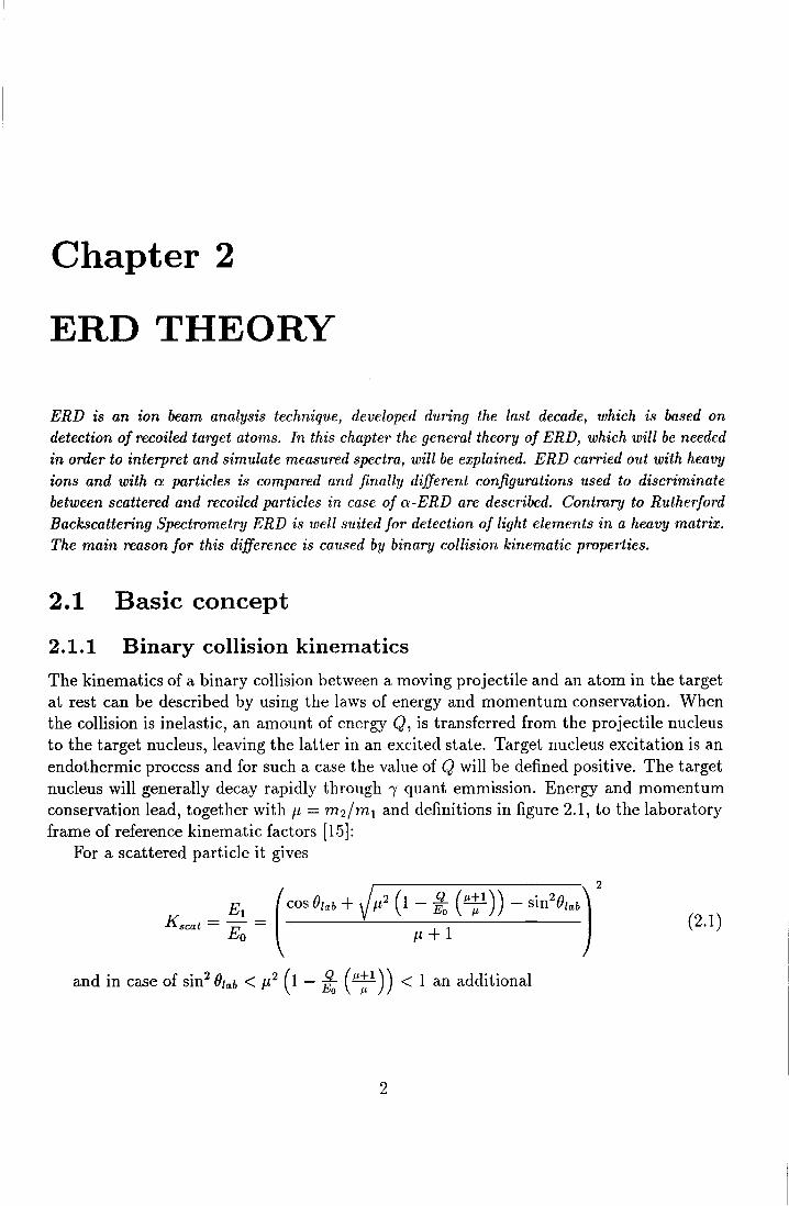
The kinematics of a binary collision between a moving projectile and an atom in the target at rest can be described by using the laws of energy and momentum conservation. When the collision is inelastic, an amount of energy Q, is transferred from the projectile nucleus to the target nucleus, leaving the latter in an excited state. Target nucleus excitation is an endothermic process and for such a case the value of Q will be defined positive. The target nucleus will generally decay rapidly through r quant emmission. Energy and momentum conservation lead, together withµ= m2/m1 and definitions in figure 2.1, to the laboratory frame of reference kinematic factors [15]:

For a scattered particle it gives

Kscat = Et = (cos 01ab + J µ2 ( 1 - £ ( ~)) - sin

2

01ab)

2

Eo µ + 1 (2.1)

and in case of sin2 01ab < µ 2 ( 1 - 2o (µ~l)) < 1 an additional

2

\

\

Figure 2.1: Laboratory frame of reference binary collision geometry.

E1 Kscat = - =

Ea (

cos B1ab - J µ2 ( 1 - fa ( 17")) - sin

201ab)

2

µ+l (2.2)

For the recoiled particles the kinematic factor equals

E2 µ 2 ( Krec = -E = 2 COS </>lab 1 ± 0 (µ + 1) )

2

1 (µ + 1) Q µEo cos2 </>1ab

(2.3)

In case of RBS or ERD with a beam of relatively heavy particles, interaction only takes place through the Coulomb force. Such binary collisions are called elastic and characterized by a Q value equal to zero. Its kinematic factors can be easily obtained by substitution of Q = 0 in formulae 2.1- 2.3.

The binary collision kinematic properties cause ERD to be better suited for detection of light elements in a heavy matrix compared to RBS. This can be illustrated with a simulated RBS spectrum and an ERD spectrum of a sample consisting of a thin BN layer on a silicon substrate, which are shown in figure 2.2. The RBS spectrum is a simulation with (} equal to 170° and a beam of 2 MeV a particles. The ERD spectrum is a simulation with 14.6 Me V a particles at an angle ef> = 30°. Complete separation between scattered and recoiled particles is assumed, therefore only recoiled particles appear in the ERD spectrum.

In the RBS spectrum the contributions of B and N are superimposed on the high silicon contribution. The advantage of ERD is that due to the kinematics the recoils emerge separated from the contribution of the substrate constituent, which improves the statistics of the measurement.

3

RBS cx-ERD

Energy (MeV) Energy (MeV) 300.2 0.4 0.6 0.8 1.0 1.2 1.4

1.0 2 4 6 8 10

B

l Si N B

25 0.8

'O 'O

~ 20 a> >= 0.6

'O 'O

-~ 15 a>

.!::! c c ~ 10

E 0.4 ....

0 0 z z

5 0.2

0 0.0 100 200 300 400 500 600 700 200 400 600 800 1000

Channel Channel

Figure 2.2: A RBS and a-ERD spectrum of a BN layer on a Si substrate.

2.1.2 Cross sections

The probability that a target atom will be recoiled in a certain solid angle df! is given by the recoiling cross section du. The same holds for scattered particles. In order to be able to quantitatively analyse an ERD spectrum the cross sections have to be known. When a projectile interacts with a target atom through the Coulomb force the recoiling cross section will be given by (refer to appendix C):

[du ] lab df! ( </J1ab) rec

(2.4)

with Z1 and Z2 representing the projectile and target atom nuclear charge respectively. The cross sections of the scattered particle can be found in appendix D.

When an ERD experiment is being carried out with a beam of high energetic (10-15 MeV) a particles the nuclear force will overwhelme the Coulomb interaction. In this case nuclear scattering will take place, which leads to a cross section deviating strongly from the Rutherford cross section.

In case of a particles this non-Rutherford behaviour will show for recoiled target atoms at an angle </J when the projectile's laboratory energy exceeds Enr, which is given by [10]:

E - 1.107 Z2 . 1 + (cos <P1abr1 (µ + 1) [MeV]

nr - A2113 ln (271/Z2) µ (2.5)

with A2 the target's atomic weight. The cross sections for both recoiled and scattered particles will depend strongly on both

the energy and the angle of recoiling or scattering respectively.

4

2.1.3 Stopping power

Another important quantity whose magnitude has to be known for good spectrum inter­pretation and simulation is the stopping power. This quantity is defined as the amount of energy a moving particle loses per unit length when travelling through a target and thereby interacting with its electrons and nuclei.

The stopping power, S, has been theoretically derived by Bethe (1930) and the non­relativistic approximation equals:

(2.6)

where 1 refers to the moving ion, being either a beam particle or a recoiled particle, and 2 to the target material. p2 denotes the target's density and I the mean excitation energy of its electrons (~10Z2 eV). Often the stopping cross section, c, is used, which is defined as:

s 2 c - N [MeV ·m] (2. 7)

with N the target atomic density. When the material is made up of more than one element, e.g. AxBy the total stopping cross section is related to the individual stopping cross sections through Bragg's rule:

tot XcA + YcB [ 2] c = MeV ·m x+y

(2.8)

Stopping powers are measured for protons and a particles [5], but in case of ERD stopping powers of heavier ions are necessary for proper spectrum simulation. Because theoretical models used for heavy ion stopping power calculation are not accurate enough, those data have to be obtained through application of Ziegler's semi-empirical data and scaling formulae [ 4].

When an ion moves through a layer with an initial energy Ei(O), its energy at depth t can be calculated with

(2.9)

or, when the stopping power is assumed to be constant and equal to the value at the initial energy, the energy is given by

(2.10)

which is called the surface approximation. The energy loss in a target is not equal for each particle due to the statistical nature of

the scattering process. This causes the energy distribution of a monoenergetic beam passing through an amount of matter to exhibit a gaussian broadening, called energy straggling. According to the Bohr theory the energy spread equals 8Es = J2rr-1 ln2 ·JNtZ2Z1 e2c01

,

with Z1 denoting the nuclear charge of the moving ion and Z2 the nuclear charge of the target atom [2].

5

2.2 a-ERD versus HI-ERD

ERD can be carried out with a beam of heavy ions, HI, like e.g. Si or with relatively light ions like e.g. a particles. Essential for ERD analysis is the discrimination between the scattered particles and recoiled particles. The major difference between HI-ERD and a-ERD is the way this discrimination takes place.

In a HI-ERD experiment the heavy scattered beam particles are often discriminated from the recoiled particles by making use of a stopper foil exploiting the difference in stopping power between the scattered and recoiled particles. The heavy scattered particles will be fully stopped in the absorber foil though the relatively light recoils will pass through. This discrimination method is rather simple and effective, but a disadvantage is the large amount of energy straggling the recoiled particles will suffer from when having travelled through the absorber foil.

In an a-ERD experiment the scattered particles and the recoils can be discriminated by exploiting their stopping power difference through application of a silicon detector with a thin sensitive layer.

The a-ERD experiments are usually carried out with a beam energy in the range of 10 - 15 MeV. These high energies lead to nuclear scattering thus a cross section which strongly depends on both the recoiling angle </> and the energy of the beam particles. The presence of these non-Rutherford cross sections provides the possibility to be sensitive for one element by making use of one of its resonance peaks with a high cross section [11]. The existence of the angular dependence of the cross section can be exploited in a more sophisticated way when e.g. a deposited layer consists of two different elements, A and B where the concentration of element A is much higher than the concentration of element B. The angle of measurement can then be chosen such that the cross section of element B is much higher than the cross section of element A, improving the detection of element B.

Compared to ERD with heavy ions a-ERD is presumed to have two advantages namely less radiation damage and a larger probing depth [6].

2.3 Element analysis with a-ERD

2.3.1 Introduction

In an a-ERD experiment the scattered and recoiled particles can be discriminated by making use of their stopping power difference. The energy deposition of a particles in a thin sensitive layer is much smaller than that of "heavy" particles like boron or carbon (refer to formula 2.6). This feature can be used to discriminate between scattered a particles and recoils.

6

2.3.2 ~E-E ERD

The most simple configuration for discrimination is using only one thin detector. This so­called ~E detector must be thick enough in order to stop all the recoils. A drawback is the huge contribution of scattered a particles which still deposit a maximum amount of energy in e.g. a 4.2 µm Si detector equal to 1.35 MeV. This results in a measurement which consists of about 98% of forwardly scattered particles. Suppression of this contribution can be achieved with the following method. During the measurement it is possible to only measure particles which deposit more energy in the ~E detector than a certain threshold. In case of a 4.2 µm Si detector this threshold equals about 1.2 MeV. In this way the contribution of the high energetic a particles, which deposit a small amount of energy in the ~E detector, can be highly suppressed, but pile-up caused by the a particles will still be present.

By putting a thick so-called E detector immediately after the ~E detector a large amount of the contribution, caused by the a particles, can be suppressed. Both signals of the ~E and E detector, which are practically coincident, are measured and stored consecutively, "in list-mode".

After the experiment the contribution of all particles which have caused a non-zero signal in the E detector, ergo the high energetic a particles, can be removed from the spectrum of the ~E detector. In case of a 4.2 µm ~E detector the maximum amount of deposited energy of a particles will decrease to approximately 1.25 Me V because a particles with an energy higher than 1.25 MeV will reach the E detector and will therefore be suppressed.

Using higher beam energies such that the recoils will no longer be stopped in the ~E detector can lead to the possibility to discriminate between different recoils having equal energy. The ratio of energies deposited by two different recoils with identical energy in a thin ~E detector is approximately equal to 2·(zt/z2 )

3 (refer to formula 2.6). In fact, each element has its own unique relationship between the deposited energy in

the ~E and in the E detector, which is visualised in figure 2.3. The usage of higher energetic beam particles will relatively improve a contribution

suppression because the maximum amount of energy deposited by the a particles in the ~E detector will remain constant though the total recoil energy will increase proportional to the beam energy. The advantage of the threshold on the ~E detector is that the spectrum of the E detector shows no large contribution of forwardly scattered a particles which ranges up to approximately E1 MeV, but instead this a contribution will only be present at very low energies, approximately up to 0.5 Me V, which improves the qualitative interpretation of the recoil contributions in the E detector spectrum.

Reconstruction of the full energy spectrum, consisting of the sum of the energy de­posited in the ~E and E detector, requires proper energy calibration of both detectors. Problems with ~E detector calibration will be discussed in chapter 4.

When the contributions of different recoiled elements appear separated in the spectrum of the ~E detector individual depth profiles can be obtained. This is achieved by selecting the contribution of one recoil in the ~E detector. After this a conditional E detector spec-

7

7,....,...,r-T""T ..................................... ~,...,...,r-T""T .................................... ~,....,...,,..,....,....

6

4

I ;

."'' .'

1'N ./·-·-·-·-·-·-·-·-·-·-·

,,,-------/ ----

/ ---

2 3 4 EE {MeV)

5 6 7

Figure 2.3: Remaining energy deposited in the E detector versus energy deposited in a 4.2 µm ~E detector for various ions.

trum containing counts which are in the selected ~E spectrum interval is generated. This spectrum shows a contribution belonging to the recoiled particles as well as a contribution which belongs to the background. By selecting the recoil contribution in both the ~E and E detector spectrum the full energy spectrum can be constructed.

2.3.3 PSD ERD

Difference in stopping power causes the a particle range to be about a decade larger than a typical C, Nor 0 range. When applying a semiconductor detector with low bias voltage the sensitive, so-called depletion layer, will be thin, but thick enough in order to stop all the recoiled particles. Yet high energetic a particles will pass through this layer and deposit an amount of energy in the neutral zone beyond this depletion layer. Both a particles and recoils will lose a certain amount of their energy through electron-hole pair creation.

Charge carriers created in the depletion layer will be collected quickly, but the charge present in the neutral zone, due to a particles, will be collected through the rather slow process of diffusion. This leads to a longer charge collection time for a particles compared to recoils. The collected charge is amplified by a preamplifier in combination with a main amplifier. The pulse shape corresponding to a high energetic a particle will be less sharpe than one corresponding to a recoiled particle. Scattered and recoiled particles can be separated by analyzing their pulse shapes with an electronic circuit.

Basically the use of a thin depletion zone with PSD ERD is equivalent to the use of a thin ~E detector with the additional advantage that the thickness of the thin sensitive layer can be varied with the applied bias voltage.

8

Chapter 3

ERD SPECTRUM SIMULATION

Interpretation of data obtained from an ERD experiment can be significantly improved with spec­trum simulation, especially when overlap of the contributions of different recoiled elements occurs. RUMP, a spectrum simulation software package, is already being used worldwide. It is designed to simulate RBS spectra and supports the simulation of ERD spectra to a limited extent, with at most two different elements which are recoiled. Its source code has been modified in order to simulate ERD spectra with an unlimited amount of recoiling elements using any kind of beam particle which includes non-Rutherford cross sections for ERD with a particles. In this chapter the spectrum calculation part of the old RUMP version will be explained as well as the changes which were necessary to make full ERD spectrum simulation possible. Some new commands which are necessary to make ERD spectrum simulations are described and finally this chapter ends with two examples of measured ERD spectra together with their simulation.

3.1 RUMP, a description

RUMP is a software package for spectrum simulation. It considers samples to be made up of a finite number of layers. In order to be able to quickly generate a proper spectrum simulation the layers are divided into thin sublayers. The surface approximation is used to calculate the energy loss of an ion in a particular su blayer [1]. The stopping powers are derived from Ziegler's semi-empirical constants and Rutherford cross sections are used to calculate each element's contribution, though non-Rutherford cross section usage is possible, in which case a cross section table containing the proper non-Rutherford cross sections will have to be loaded.

RUMP has been especially developed for RBS spectrum simulation but it is also capable of ERD spectrum simulation, yet in a limited way. Only HI-ERD spectra with Ruther­ford cross sections can be simulated and moreover, these spectra can contain at most the contributions of no more than two different recoiled elements.

9

Energy

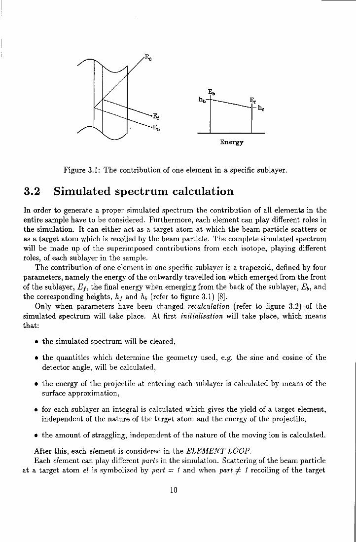
Figure 3.1: The contribution of one element in a specific sub layer.

3.2 Simulated spectrum calculation

In order to generate a proper simulated spectrum the contribution of all elements in the entire sample have to be considered. Furthermore, each element can play different roles in the simulation. It can either act as a target atom at which the beam particle scatters or as a target atom which is recoiled by the beam particle. The complete simulated spectrum will be made up of the superimposed contributions from each isotope, playing different roles, of each sublayer in the sample.

The contribution of one element in one specific sublayer is a trapezoid, defined by four parameters, namely the energy of the outwardly travelled ion which emerged from the front of the sublayer, Eh the final energy when emerging from the back of the sublayer, Eb, and the corresponding heights, h f and hb (refer to figure 3.1) [8].

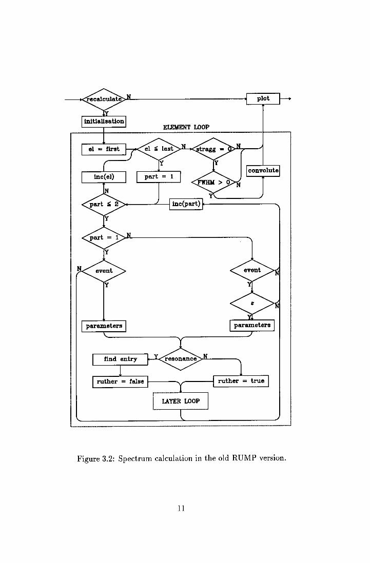
Only when parameters have been changed recalculation (refer to figure 3.2) of the simulated spectrum will take place. At first initialisation will take place, which means that:

• the simulated spectrum will be cleared,

• the quantities which determine the geometry used, e.g. the sine and cosine of the detector angle, will be calculated,

• the energy of the projectile at entering each sublayer is calculated by means of the surface approximation,

• for each sublayer an integral is calculated which gives the yield of a target element, independent of the nature of the target atom and the energy of the projectile,

• the amount of straggling, independent of the nature of the moving ion is calculated.

After this, each element is considered in the ELEA1ENT LOOP. Each element can play different parts in the simulation. Scattering of the beam particle

at a target atom el is symbolized by part = 1 and when part # 1 recoiling of the target

10

plot

initialisation ELEMENT LOOP

el = first

convolute inc(el) 1

~--.-L-----1 inc(part) 11----------...

parameters

find entry

ruther = false i----- ------i ruther = true

[ _______ , __ ....... __ ~_YE_R_LO_OP-·----· __ __.

Figure 3.2: Spectrum calculation in the old RUMP version.

11

LAYER LOOP

lay = top

inc(lay)

add

convolute

I L

Rutherford u low energy I ------------ -------------------------·

Figure 3.3: The layer loop.

atom el is considered. In both cases event symbolizes a check whether the event can take place at all. E.g. in case of recoiling it checks whether the detector angle </>is smaller than 90°. Furthermore, in case of recoil calculation RUMP checks whether the stopping power of the element is present in the currently loaded stopping power table,€. Finally, parameters necessary for calculation of the elements contribution, like the kinematic factor and the energy independent factor of the Rutherford cross section are calculated. The existence of the proper resonance cross section table is checked. If it is present the required entry is looked for and the boolean ruther is set false, otherwise ruther is set true.

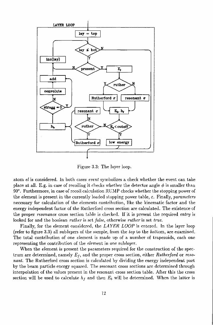
Finally, for the element considered, the LA YER LOOP is entered. In the layer loop (refer to figure 3.3) all sublayers of the sample, from the top to the bottom, are examined. The total contribution of one element is made up of a number of trapezoids, each one representing the contribution of the element in one sublayer.

When the element is present the parameters required for the construction of the spec­trum are determined, namely Ef, and the proper cross section, either Rutherford or reso­nant. The Rutherford cross section is calculated by dividing the energy independent part by the beam particle energy squared. The resonant cross sections are determined through interpolation of the values present in the resonant cross section table. After this the cross section will be used to calculate h f and then Eb will be determined. When the latter is

12

lower than cutoff, which equals 100 ke V, the stopping powers used to determine Eb will not be accurate enough. In that case a low energy spectrum construction routine is called. In all other cases the the proper cross section will be calculated, which will be used for determination of hb. Only when straggling should be taken into account, the contribution will be convoluted with a gaussian with width equal to the sum of both the straggling magnitude and the detector resolution. Finally, the contribution of the element is added to the spectrum.

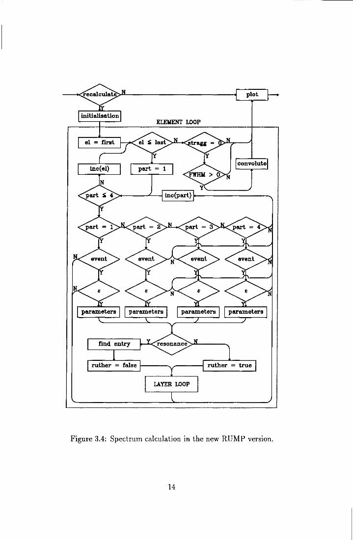
When all elements are considered and straggling should not be taken into account a non-zero detector resolution FW H M > 0 will result in convolving the spectrum with a gaussian of width equal to FWHM. The last step is plotting the spectrum on the standard output device.

3.3 Changes to RUMP

In order to allow rigorous ERD simulation the following modifications of the RUMP source code have to be implemented:

• Selecting the ions which are displayed following the calculation i.e. either recoils or scattered particles or both. This is necessary to e.g. implement simulation of a-ERD or HI-ERD with a magnetospectrograph. Selection of the type of spectrum to be calculated can be done with the command SIM XPTYpe which will be described in subsection 3.4.1. Furthermore, the source code has to be modified in order to calculate the different spectra. Figure 3.4 shows the changed spectrum calculation part. The part loop has been extended and the roles of the different parts have been changed. Part = 1 now represents scattered particles withµ < 1, part = 2 calculates the contribution of scattered particles with a kinematic factor given in formula 2.1, in which case the cross section deviates from the normal Rutherford scattering cross section (refer to appendix D), whilst part = 3 represents the scattered particles with µ > 1 and a kinematic factor given in formula 2.2. The contribution of recoiled particles is being calculated in part 4.

• Implementation of loading stopping powers when they are necessary for simulation but not available. This has to be done in a separate routine which loads those tables. When during simulation stopping powers are needed and not present, the new RUMP version automatically attempts loading them. This implies that fixed names for tables which contain data for certain elements have been defined, these names are given in appendix B. Because of the diversity of experimental conditions a tool to generate such stopping power tables, STOPP, is present. A short description of STOPP can be found in appendix A.

• Implementation of the ability to simulate non-Rutherford recoiling, which takes place in case of a-ERD. RUMP already is able to simulate non-Rutherford scattering, using tables containing scattering cross sections which can be obtained from literature. In

13

plot

initialisation ELEMENT LOOP

el = first

inc(el) convolute

~----"'------! inc{part) ...---------......

find entry

ruther = false i-----.... ___ __, ruther = true

LAYER LOOP I .______. , .............................................. -~ J

___________ !_ ____ , ....... - ........ __ ..... __

Figure 3.4: Spectrum calculation in the new RUMP version.

14

order to maintain compatibility with the existing RUMP version, the recoiling cross sections will be derived from the scattering cross sections of the same collision. Tables containing non-Rutherford scattering cross sections can be generated by RES5, which is described in appendix A.

• Simulation of straggling in both the stopper foil and the sample. With the already existing, limited ERD spectrum simulation routine it was not possible to take strag­gling of the recoiled particles into account. In the new version not only straggling in the sample, but also in the stopper foil, especially useful for HI-ERD simulation, has been implemented. The magnitude of straggling is calculated according to the Bohr theory. RUMP actually calculates VIBs which is proportional to the pathlength. When a stopper foil is used, the amount of straggling due to this foil will be simply added to the current amount of straggling, caused by the sublayers of the sample. The change has been made in the layer loop.

• Introduction of the scaling of the stopping power of a moving ion. The stopping powers of ions heavier than He, derived from Ziegler's semi-empirical data can deviate up to 20% from their actual stopping power. Therefore simulations do not always fit the experimental data.

The stopping power of a moving ion depends on the state of both the ion and the matter it moves through. Scaling of the stopping power of the target matter could already be performed by RUMP with the SCale command. In the new RUMP version a new command has been implemented, SIM SCION, which allows scaling the stopping power of the moving ion. SIM SCION will be described in subsection 3.4.3.

Furthermore, after loading a new stopping power table by means of the LOAD com­mand scaling through both the SCale and the SCION command will be maintained.

3.4 New commands

In order to be able to use the modified RUMP version a few commands, which will be explained below, have been implemented.

3.4.1 Xptype

In order to be able to simulate e.g. spectra obtained through a-ERD experiments or HI­ERD experiments with a magnetospectrograph the particles to be displayed, either scat­tered or recoiled or both, have to be choosen.

15

This can be done by entering the SIM command XPTYpe [n]. Three options are available:

0 Spectrum simulation with only scattered particles,

1 Spectrum simulation with only recoiled particles,

2 Complete spectrum simulation with both scattered as well as recoiled particles.

The XPTYpe 0 mode is exquisite for RBS simulation and equivalent to the previous RUMP version in both speed and appearance. Contributions of merely the recoiled sample constituents appear in XPTYpe 1 mode, which is suited for ERD simulation. Finally, the XPTYpe 2 mode provides a spectrum with both scattered and recoiled particles.

RBS and ERD experiments are usually carried out with different beam particles and energies. Therefore it is useful to have separate stopping power tables for RBS and ERD.

In case of RBS there is only one table which is named rbsbeam.dat and automatically loaded when XPTYpe 0 is specified. This table should contain stopping power data for three often used beam particles for RBS experiments. In most cases this table will replace atom3.dat, the commonly used table containing stopping powers for hydrogen, deuterium and helium.

In case of ERD the stopping power table with data for three often used beam particles is named erdabeam.dat and automatically loaded when XPTYpe 1 is specified. Further­more, tables exist with stopping power data for sets of three elements. The names of the tables are given in appendix B. During ERD simulation these stopping power tables will be automatically loaded when necessary.

3.4.2 Recoil

RUMP originally has been designed for one purpose, rapid RBS spectrum simulation using Rutherford cross sections. Though at a later stage, non-Rutherford scattering has been implemented. Because non-Rutherford cross sections are given in the literature as a func­tion of the beam energy for a fixed scattering angle, RUMP uses tables, labeled by this scattering angle, containing those cross sections.

Now also simulation of resonant recoiling has been implemented. In order to maintain compatibility with the existing RUMP version the resonant recoiling cross sections will be derived from the resonant scattering cross sections of the same event, which are available in the literature. This has two consequences:

• RUMP has to know the proper scattering angle () belonging to the requested recoil angle </> in order to be able to look for the right resonant scattering cross section table. Furthermore this scattering cross section has to be transformed into the recoiling cross section, which requires a geometrical conversion factor. This conversion factor is equal to:

16

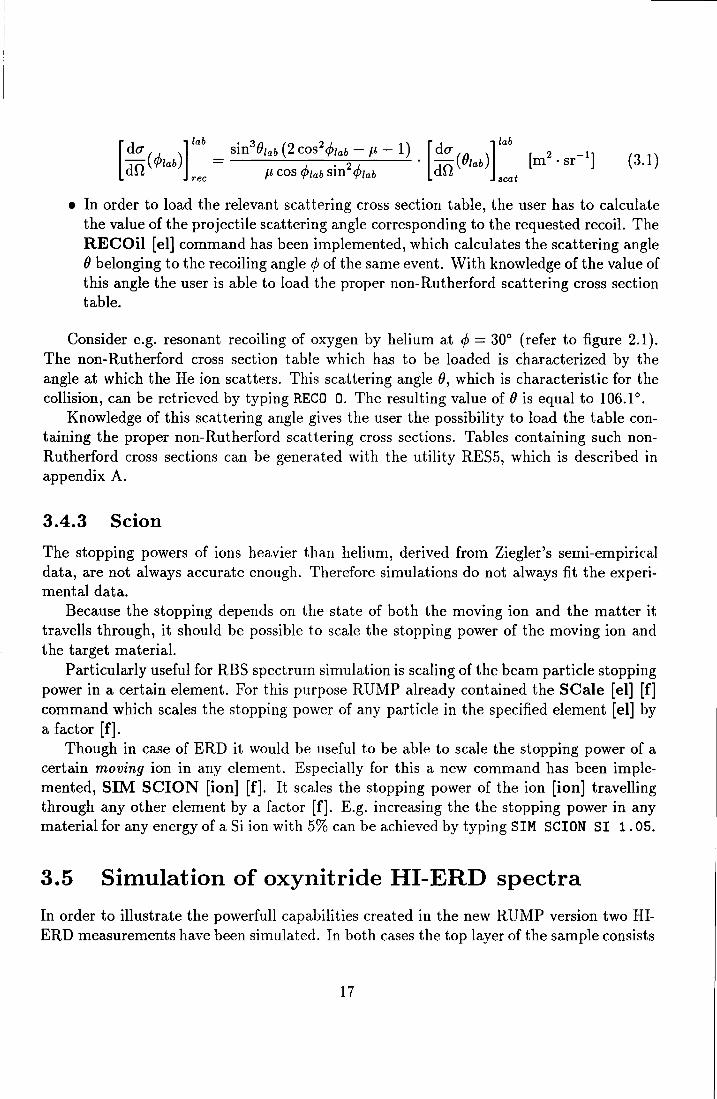
[d0"(</>1ab)llab = sin301ab(2cos2</>~ab2-µ-l). [du(01ab)llab [m2·sr-1] (3.1) an µ cos </>lab sm </>1ab an t rec sea

• In order to load the relevant scattering cross section table, the user has to calculate the value of the projectile scattering angle corresponding to the requested recoil. The RECOil [el] command has been implemented, which calculates the scattering angle 0 belonging to the recoiling angle </> of the same event. With knowledge of the value of this angle the user is able to load the proper non-Rutherford scattering cross section table.

Consider e.g. resonant recoiling of oxygen by helium at </> = 30° (refer to figure 2.1). The non-Rutherford cross section table which has to be loaded is characterized by the angle at which the He ion scatters. This scattering angle 0, which is characteristic for the collision, can be retrieved by typing RECO 0. The resulting value of 0 is equal to 106.1°.

Knowledge of this scattering angle gives the user the possibility to load the table con­taining the proper non-Rutherford scattering cross sections. Tables containing such non­Rutherford cross sections can be generated with the utility RES5, which is described in appendix A.

3.4.3 Scion

The stopping powers of ions heavier than helium, derived from Ziegler's semi-empirical data, are not always accurate enough. Therefore simulations do not always fit the experi­mental data.

Because the stopping depends on the state of both the moving ion and the matter it travells through, it should be possible to scale the stopping power of the moving ion and the target material.

Particularly useful for RBS spectrum simulation is scaling of the beam particle stopping power in a certain element. For this purpose RUMP already contained the SCale [el] [f] command which scales the stopping power of any particle in the specified element [ el] by a factor [ f].

Though in case of ERD it would be useful to be able to scale the stopping power of a certain moving ion in any element. Especially for this a new command has been imple­mented, SIM SCION [ion] [f]. It scales the stopping power of the ion [ion] travelling through any other element by a factor [f]. E.g. increasing the the stopping power in any material for any energy of a Si ion with 5% can be achieved by typing SIM SCION SI 1. 05.

3.5 Simulation of oxynitride HI-ERD spectra

In order to illustrate the powerfull capabilities created in the new RUMP version two HI­ERD measurements have been simulated. In both cases the top layer of the sample consists

17

2 3 6

5 ·· · · ·· e][J>eriment -theory

"U

.~ 4 H >-"U

.§ 3 0 E L... 2 0 z

0 ... ·~·.- ~

100 200

Energy (MeV) 4

0

300

5

400 Channel

6

N

500

7 8

600 700

Figure 3.5: HI-ERD spectrum of a silicon oxynitride film on Si.

of a silicon oxynitride mixture containing hydrogen [7]. The bulk material is silicon and in the second sample the top layer and bulk are separated by a thermally grown Si02 layer.

Figure 3.5 shows the measured ERD spectrum of the first sample together with the RUMP simulation. This recoil spectrum is measured using a 30 Me V 28Si ion beam at an angle of </> = 36°. During the experiment a 9 µm mylar stopper foil was used to stop the scattered Si beam particles. According to the simulation the top layer consists of 300· 1015 atoms·cm-2 Si3 N i.s01.3H0.6 • The simulation has been performed with a detector resolution of 100 ke V and straggling equal to 10 times the Bohr straggling. Stopping power scaling was not necessary for proper fitting because the oxynitride layer was very thin. During the simulation different stopping power tables have been loaded and Rutherford cross sections have been used to calculate the contribution of the recoiled ions.

The sharp peak is caused by a small amount of hydrogen in the oxynitride layer. Kine­matically, oxygen has a higher energy than nitrogen but difference in stopping of nitrogen and oxygen in the absorption foil causes them to be reversed on the energy axis. Note the slope of the high energy side of both the nitrogen and oxygen contribution which is caused by straggling in the stopper foil.

The measurements on the second sample have been carried out at a recoil angle</>= 34° with a 30 Me V 28Si beam. Again a mylar stopper foil has been used to discriminate between the scattered and recoiled particles.

The results of this measurement together with the simulation are shown in figure 3.6.

18

....... =--' H = = = = :: ::

one calibration

II 0

600 Channel

:s 6 G)

>= '1:1

N r ~2

800 0

200

element dependent calibration

H

0 N

0

400 600 800 Channel

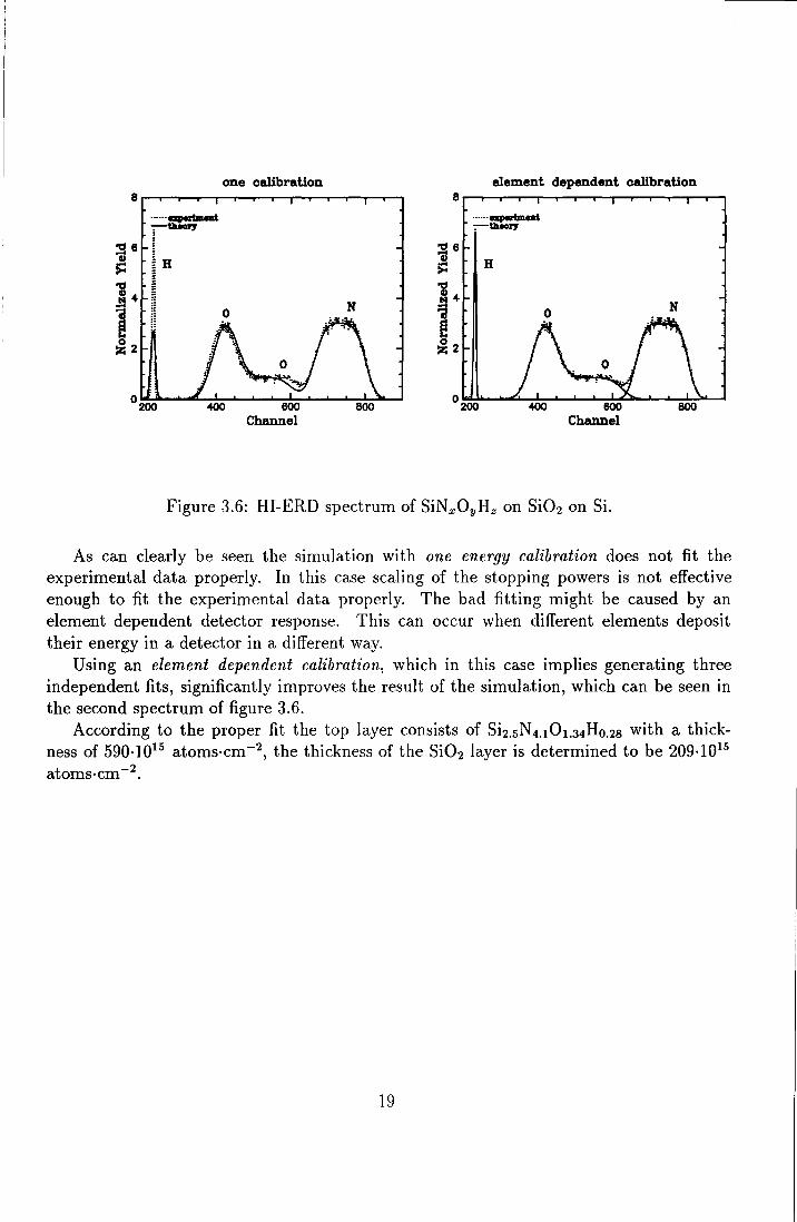
Figure 3.6: HI-ERD spectrum of SiNxOyHz on Si02 on Si.

As can clearly be seen the simulation with one energy calibration does not fit the experimental data properly. In this case scaling of the stopping powers is not effective enough to fit the experimental data properly. The bad fitting might be caused by an element dependent detector response. This can occur when different elements deposit their energy in a detector in a different way.

Using an element dependent calibration, which in this case implies generating three independent fits, significantly improves the result of the simulation, which can be seen in the second spectrum of figure 3.6.

According to the proper fit the top layer consists of Si2.5N4.1 Oi.34H0.28 with a thick­ness of 590· 1015 atoms·cm-2, the thickness of the Si02 layer is determined to be 209· 1015

atoms·cm-2.

19

Chapter 4

EXPERIMENTS

The feasibility of .6.E-E ERD and pulse shape discrimination (PSD) ERD using a projec­tiles has been investigated by carrying out experiments on thin (-;::::, 100 nm) Bx Ny Hz layers and thick (-;:::,J µm) CxNyHz layers on a silicon substrate. These measurements have been used to compare the methods of both .6.E-E ERD and PSD ERD.

The .6.E-E measurements on the BxNyHz layer on silicon have also been used to deter­mine the effective boron cross section as a function of the recoiling angle </>.

Both samples have also been investigated with simultaneous conventional ERD and RBS measurements, with a beam of 4 Me Va particles and a stopper foil in front of the ERD detector, to determine the amount of hydrogen in the layers.

Furthermore, simulation of the RBS measurements provide an estimate of the thickness of the BxNyHz and CxNyHz layer on Si.

4.1 Introduction

All ERD measurements have been carried out with the geometry shown in figure 4.1. In case of .6.E-E ERD the detector is a combination of a 4.2 µm .6.E surface barrier detector with a thick E Si PIPS detector behind it. For the PSD ERD experiments a Si PIPS detector is used and in a conventional ERD experiment the detector consists of a thin stopper foil with a Si PIPS detector behind it.

Both samples contained nitrogen, so in order to have a high cross section for nitrogen recoiling the beam energy used during the experiments was 14.6 MeV. The angle between the incident beam of a particles and the normal of the sample, 01 , is 75°. During the experiments the recoil angle </> can be varied by repositioning the detector. The pressure in the scattering chamber is held at 10-3 Pa.

4.2 Hydrogen

In order to determine the amount of hydrogen in the BxNyHz and CxNyHz layer on Si conventional ERD and RBS measurements have been carried out simultaneously using a

20

incident

a beam

sample

....

detector

0 . ...

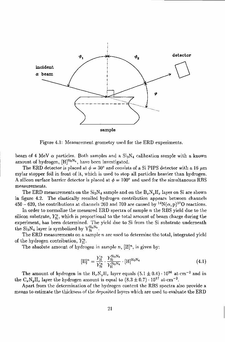
Figure 4.1: Measurement geometry used for the ERD experiments.

beam of 4 MeV a particles. Both samples and a Si3N4 calibration sample with a known amount of hydrogen, [H]Si3N4, have been investigated.

The ERD detector is placed at</>= 30° and consists of a Si PIPS detector with a 16 µm mylar stopper foil in front of it, which is used to stop all particles heavier than hydrogen. A silicon surface barrier detector is placed at </> = 100° and used for the simultaneous RBS measurements.

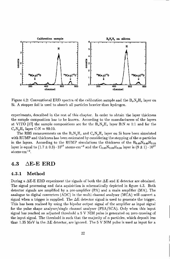
The ERD measurements on the Si3 N4 sample and on the BxNyHz layer on Si are shown in figure 4.2. The elastically recoiled hydrogen contribution appears between channels 450 - 620, the contributions at channels 260 and 700 are caused by 14N (a, p) 17 0 reactions.

In order to normalize the measured ERD spectra of sample n the RBS yield due to the silicon substrate, YSi, which is proportional to the total amount of beam charge during the experiment, has been determined. The yield due to Si from the Si substrate underneath the SbN4 layer is symbolized by Y~j3N4 •

The ERD measurements on a sample n are used to determine the total, integrated yield of the hydrogen contribution, Yi!.

The absolute amount of hydrogen in sample n, [H]n, is given by:

y;n y:;Si3N4 [H]n = _!!_ . Si. . [H]SiJN4 (4.1)

'.l"n ,7S13N4 Igj IH

The amount of hydrogen in the BxNyIIz layer equals (5.1±0.4) · 1016 at·cm-2 and in the CxNyHz layer the hydrogen amount is equal to (8.3 ± 0.7) · 1017 at·cm-2

.

Apart from the determination of the hydrogen content the RBS spectra also provide a means to estimate the thickness of the deposited layers which are used to evaluate the ERD

21

3

!'J ~2 0 ()

Calibration sample

H

o.__..-..-......:i..-.....-...---_._--........ ~......_. 200 400 600 800

channel

'.BzN,Hs on silicon 5,.........,,.........-...._,._,..._. __________ ...._~

5

!'J ~3 0 ()

2

1'N(cx,p)110

.i.

H

Figure 4.2: Conventional ERD spectra of the calibration sample and the BxNyHz layer on Si. A stopper foil is used to absorb all particles heavier than hydrogen.

experiments, described in the rest of this chapter. In order to obtain the layer thickness the sample composition has to be known. According to the manufacturers of the layers at VITO [17] the sample compositions are for the BxNyHz layer B:N::::::: 1:1 and for the CxNyHz layer C:N::::::: 90:10.

The RBS measurements on the BxNyHz and CxNyHz layer on Si have been simulated with RUMP and thickness has been estimated by considering the stopping of the a particles in the layers. According to the RUMP simulations the thickness of the B0 .49No.49H0 .03

layer is equal to (1.7 ± 0.3) · 1017 atoms·cm-2 and the C0.83N0 .09H0.08 layer is (9 ± 1) · 1017

atoms·cm-2•

4.3 LiE-E ERD

4.3.1 Method

During a ~E-E ERD experiment the signals of both the ~E and E detector are obtained. The signal processing and data aquisistion is schematically depicted in figure 4.3. Both detector signals are amplified by a pre-amplifier (PA) and a main amplifier (MA). The analogue to digital converters (ADC) in the multi channel analyser (MCA) will convert a signal when a trigger is supplied. The ~E detector signal is used to generate the trigger. This has been realised by using the bipolar output signal of the amplifier as input signal for the pulse shape analyser/single channel analyser (PSA/SCA). Only when this input signal has reached an adjusted threshold a ,5 V NIM pulse is generated on zero crossing of the input signal. The threshold is such that the majority of a particles, which deposit less than 1.35 Me V in the ~E detector, are ignored. The 5 V NIM pulse is used as input for a

22

data server

PHYBUS

VME BUS

PHYLAN

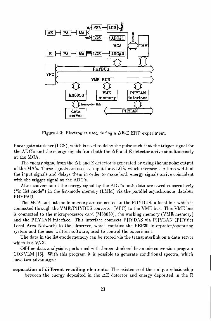
Figure 4.3: Electronics used during a ~E-E ERD experiment.

linear gate stretcher (LGS), which is used to delay the pulse such that the trigger signal for the ADC's and the energy signals from both the ~E and E detector arrive simultaneously at the MCA.

The energy signal from the ~E and E detector is generated by using the unipolar output of the MA's. These signals are used as input for a LGS, which increase the time-width of the input signals and delays them in order to make both energy signals arrive coincident with the trigger signal at the ADC's.

After conversion of the energy signal by the ADC's both data are saved consecutively ("in list mode") in the list-mode memory (LMM) via the parallel asynchronous databus PHYPAD.

The MCA and list-mode memory are connected to the PHYBUS, a local bus which is connected through the VME/PHYBUS converter (VPC) to the VME bus. This VME bus is connected to the microprocessor card (l'v168030), the working memory (VME memory) and the PHYLAN interface. This interface connects PIIYDAS via PHYLAN (PHY sics Local Area Network) to the fileserver, which contains the PEP30 interpreter/operating system and the user written software, used to control the experiment.

The data in the list-mode memory can be stored via the transputerlink on a data server which is a VAX.

Off-line data analysis is performed with Jeroen Jonkers' list-mode conversion program CONVLM [16]. With this program it is possible to generate conditional spectra, which have two advantages:

separation of different recoiling elements: The existence of the unique relationship between the energy deposited in the ~E detector and energy deposited in the E

23

AE detector E detector 400

JOO 300

!J !J § 200 B § 200 0 ()

0 ()

B 100 N 100

0500 1000 1500 2000 2500 3000 3500 00 2000 3000 4000 channel channel

Figure 4.4: ~E and E detector spectra of BxNyHz on Si at </> = 30°.

detector for each element provides the possibility to separate the contributions of different recoiling elements even when they have equal energies. This separation can be achieved by generation of conditional spectra.

separation of recoiling elements from the a contribution: Contributions of recoiled elements can appear superimposed on a background, caused by e.g. the forwardly scattered a particles. With generation of conditional spectra the recoil contribution can be separated from this background.

In order to obtain depth profiles of a recoiling element the spectrum of yield versus the total energy of the recoil has to be known. The total energy of a recoiled ion is equal to the sum of the energy deposited in the ~E detector and the energy deposited in the E detector. This total energy can only be calculated when both detectors are calibrated properly.

4.3.2 ~E-E ERD measurements on a BxNyHz layer on Si

In order to be able to compare the performance of ~E-E ERD for layers with different thicknesses, a sample consisting of a thin (~100 nm) BxNyHz layer on a silicon substrate has been investigated at recoil angles </> ranging from 30° to 50°. These measurements will be compared to the ~E-E ERD measurements on the thick (~l µm) CxNyHz layer on silicon, which will be described in subsection 4.3.3.

24

Recoil separation with the ~E-E telescope

For a recoil angle </> = 30° the ~E and E detector spectra are shown in figure 4.4. The ~E detector spectrum clearly shows the elastically B and N and inelastically recoiled N* contributions on a background. This background can be caused by different effects:

• pile-up due to two or more a particles entering the ~E detector simultaneously and depositing enough energy to generate a trigger.

• carbon ions recoiled from the slits of the beam guiding system which are scattered at the target or target holder. Their maximum total energy would be ~10 MeV. But all carbon ions in the energy range of 5.5 - 8.2 Me V deposit ( 5.1 ± 0.1) Me V in the thin ~E detector and should appear between the boron and nitrogen contribution, causing a distinct peak, yet such a peak is clearly absent in the ~E detector spectrum. Therefore the contribution of carbon recoils is unlikely to cause the background in the ~E detector spectrum.

• silicon recoils from the substrate. At the interface their energy would be 4.9 MeV, but according to the RUMP simulation the final energy would be 3.0 MeV, which means that it should appear left from the boron contribution.

• electronic noise caused by the detector or electronic circuit.

In the ~E detector spectrum the boron contribution appears left from the nitrogen contribution. The energy of boron ions from the surface (8.93 MeV) is higher than the energy of nitrogen ions from the surface (7.56 MeV), but the stopping power of boron being lower than the nitrogen stopping power causes boron to deposit less energy in the ~E detector compared to nitrogen. Between the boron and nitrogen peak the contribution due to the first excited state of the 14N nucleus (Q = 2.3129 MeV) is also visible. The high contribution at channel 500 - 1000 is caused by low energetic a particles (Ea ~ 1.35 MeV) which are scattered from deep in the target.

In the E detector spectrum the boron peak is visible on a background. This background is caused by pile-up due to high energetic a particles which enter the ~E detector coin­cidently with a particle, either a low energetic a particle or a recoil, which will generate a trigger for the ADC's. The channel at which the high energy edge of the background appears corresponds, according to the calibration in equation 4.4, to the maximum energy an a particle can deposit in the E detector. The contribution of the background due to a particles can be reduced by increasing the threshold on the ~E detector such that no a particle will be able to generate a trigger for the ADC.

The contribution due to the recoiled nitrogen ions from the surface, which pass through the ~E detector, cannot be seen in the E detector spectrum, because it overlaps with the high contribution of forwardly scattered a particles at channel 0 - 400, which were able to generate a trigger in the ~E detector.

Fortunately it is possible to separate the contributions of the recoiled elements from the background by generation of conditional spectra.

25

boron nitrogen 80 80

50 ex 50 N

40 us- l°J3+nB+l°J3•

40

• • §30 .... ~JO

0 0 () ()

20 20

10 10

00 1000 1500 500 1000 1500 2000 channel channel

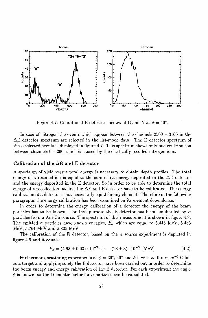
Figure 4.5: Conditional E detector spectra of B and N at </> = 30°.

In case of boron all events which appear between the channels 1500 - 2200 in the ~E detector spectrum are selected in the list-mode data and the E detector spectrum of these selected events is displayed in figure 4.5. This spectrum shows three peaks. The contribution between channel 800 - 1300, caused by the elastically recoiled 10B and 11 B ions, together with inelastically recoiled 10B*, whose first excited state has a Q value equal to 0.7183 MeV, resulting in an energy of 8.53 MeV, therefore overlapping with the 11 B contribution of 8.57 MeV.

The contribution of the inelastically recoiled boron 11 B** nuclei, between channel 200 -700, is caused by the second excited state which has a Q value equal to 4.4451 MeV. This contribution was not separately visible in the ~E detector spectrum because it overlapped with the elastically recoiled 10B and 11 B ions. The contribution appearing between the channels 0 - 300 is due to the background in the ~E detector spectrum.

In case of nitrogen the events which appear between the channels 2700 - 3300 in the ~E detector spectrum are selected in the list-mode data. The E detector spectrum of these selected events is displayed in figure 4.5. This spectrum shows two contributions. Between channels 100 - 500 the elastically recoiled nitrogen contribution appears and at channels lower than 100 a small contribution due to the background in the ~E detector spectrum is visible.

~E and E detector spectra have been recorded at 11 recoiling angles between 30° and 50° in order to calibrate the ~E detector and determine the angular dependence of the effective boron recoiling cross section. By varying the recoiling angle </> the kinematic factor and therefore the energies of the different recoiling elements change. This can be illustrated with e.g. spectra measured at </> = 40°, which are given in figure 4.6.

The ~E detector spectrum shows the B and N contributions on a background. The energy of a boron recoil from the surface of the BxNyHz layer is equal to 6.98 MeV. With

26

AE detector E detector 200 200

150 150

N

.!! B .!! ~ 100 ~ 100 0 0 0 0 B

50 50

0500 1000 00

Figure 4.6: ~E and E detector spectra of BxNyHz on Si at <P = 40°.

figure 2.3 it follows that the energy deposited in the ~E detector should be approximately equal to the deposited energy at <P = 30° and compared to the ~E detector spectrum at 30°, shown in figure 4.4, the boron peak indeed appears at the same channel interval.

Nitrogen recoils emerging from the surface of the layer have a total energy equal to 5.92 MeV and, as can be deduced from figure 2.3, the energy deposited in the ~E detector should be less than the amount deposited at 30°. When comparing both ~E detector spectra, shown in figures 4.4 and 4.6, the top of the nitrogen contribution has indeed shifted about 100 channels to 2850. The contribution of the first excited state of 14N has vanished from the ~E detector spectrum because of its low recoiling cross section at <P = 40°. The high contribution between channels 500 - 800 is ca11sed by low energetic a particles which are scattered from deep in the target.

In the E detector spectrum, shown in figure 4.6, the boron peak is visible on a small background. Similar to the spectra at 30° it is possible to separate the contributions of the recoiled elements from the background by generation of conditional spectra.

In case of boron all events which appear between the channels 1600 - 2000 in the ~E detector spectrum are selected in the list-mode data. The E detector spectrum of these selected events is displayed in figure 4. 7. This spectrum surprisingly shows three peaks. The contribution between channel 550 - 800, caused by the elastically recoiled 10B and 11 B ions, together with the inelastically recoiled 10B nuclei. The inelastically recoiled boron, 11B*, between channel 300 - 550, caused by the first excited state of the 11B nucleus (Q = 2.1247 MeV) and 11 B**, between channel 0 - 200, caused by the second excited state of the 11 B nucleus. These contributions were not separately visible in the ~E detector spectrum because they overlapped with the elastically recoiled 10B and 11 B ions. A fraction of the contribution appearing between the channels 0 - 200 will be due to the background in the ~E detector spectrum.

27

boron nitrogen 60 200

10s+nB+1°B• 50

150 40

!J !J § 30 § 100 0 0 () ()

20 50

10

1000 250 300

Figure 4.7: Conditional E detector spectra of Band Nat <P = 40°.

In case of nitrogen the events which appear between the channels 2500 - 3100 in the ~E detector spectrum are selected in the list-mode data. The E detector spectrum of these selected events is displayed in figure 4. 7. This spectrum shows only one contribution between channels 0 - 200 which is caused by the elastically recoiled nitrogen ions.

Calibration of the ~E and E detector

A spectrum of yield versus total energy is necessary to obtain depth profiles. The total energy of a recoiled ion is equal to the sum of its energy deposited in the ~E detector and the energy deposited in the E detector. So in order to be able to determine the total energy of a recoiled ion, at first the ~E and E detector have to be calibrated. The energy calibration of a detector is not necessarily equal for any element. Therefore in the following paragraphs the energy calibration has been examined on its element dependence.

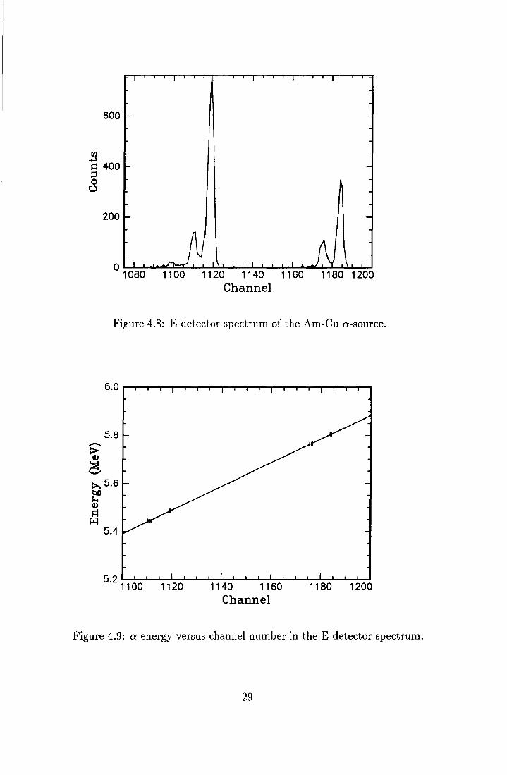
In order to determine the energy calibration of a detector the energy of the beam particles has to be known. For that purpose the E detector has been bombarded by a particles from a Am-Cu source. The spectrum of this measurement is shown in figure 4.8. The emitted a particles have known energies, Ea which are equal to 5.443 MeV, 5.486 MeV, 5.764 MeV and 5.805 MeV.

The calibration of the E detector, based on the a source experiment is depicted in figure 4.9 and it equals:

Ea= (4.93 ± 0.03) · 10-3 ·eh - (28 ± 3) · 10-3 [MeV] ( 4.2)

Furthermore, scattering experiments at <P = 30°, 40° and 50° with a 10 mg·cm-2 C foil as a target and applying solely the E detector have been carried out in order to determine the beam energy and energy calibration of the E detector. For each experiment the angle <P is known, so the kinematic factor for a particles can be calculated.

28

fll ...,

600

r:: 400 ::s 0 u

200

0 1080 1100 1120 1140 1160 1180 1200

........... > Q)

~ ...._..

Channel

Figure 4.8: E detector spectrum of the Am-Cu a-source.

5.8

:;:.... 5.6 bll J.i Q)

r:: ~

5.4

5.2 ___ .........,.........,........., ______________ __...._

11 00 11 20 11 40 11 60 1180 1 200

Channel

Figure 4.9: a energy versus channel number in the E detector spectrum.

29

0.95

0.90

.i J0.85

0.80

0.75

0·10

2300 2400 2500 2600 2700 2800 Channel

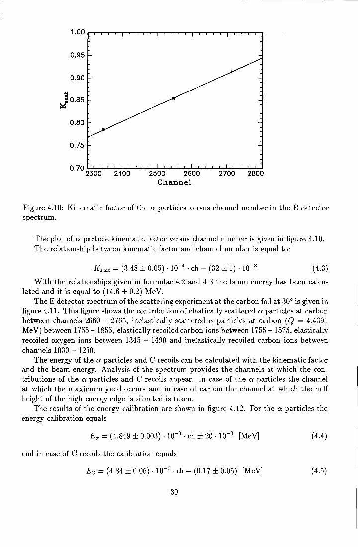
Figure 4.10: Kinematic factor of the a particles versus channel number in the E detector spectrum.

The plot of a particle kinematic factor versus channel number is given in figure 4.10. The relationship between kinematic factor and channel number is equal to:

I<scat = (3.48 ± 0.05). 10-4• eh - (32 ± 1). 10-3 ( 4.3)

With the relationships given in formulae 4.2 and 4.3 the beam energy has been calcu­lated and it is equal to (14.6 ± 0.2) MeV.

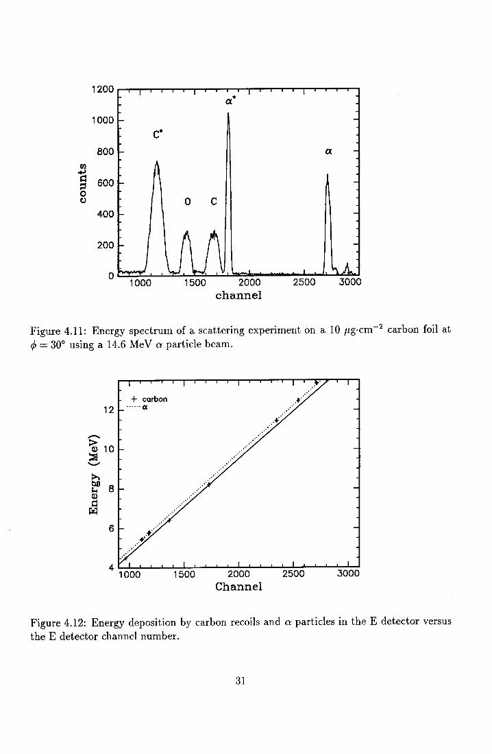
The E detector spectrum of the scattering experiment at the carbon foil at 30° is given in figure 4.11. This figure shows the contribution of elastically scattered a particles at carbon between channels 2660 - 2765, inelastically scattered a particles at carbon ( Q = 4.4391 MeV) between 1755 - 1855, elastically recoiled carbon ions between 1755 - 1575, elastically recoiled oxygen ions between 1345 - 1490 and inelastically recoiled carbon ions between channels 1030 - 1270.

The energy of the a particles and C recoils can be calculated with the kinematic factor and the beam energy. Analysis of the spectrum provides the channels at which the con­tributions of the a particles and C recoils appear. In case of the a particles the channel at which the maximum yield occurs and in case of carbon the channel at which the half height of the high energy edge is situated is taken.

The results of the energy calibration are shown in figure 4.12. For the a particles the energy calibration equals

Ea = ( 4.849 ± 0.003) · 10-3 ·eh± 20 · 10-3 [MeV] ( 4.4)

and in case of C recoils the calibration equals

Ee = (4.84 ± 0.06) · 10-3 ·eh - (0.17 ± 0.05) [MeV] ( 4.5)

30

1200 • ex

1000 c·

800 ex

l1l ~ ~ 600 = 0 t> 0 c

400

200

0 1000 1500 2000 2500 3000

channel

Figure 4.11: Energy spectrum of a scattering experiment on a 10 µg·cm- 2 carbon foil at <P = 30° using a 14.6 MeV a particle beam.

+ carbon 12 ······a

6

4 1000 1500 2000

Channel 2500 3000

Figure 4.12: Energy deposition by carbon recoils and a particles in the E detector versus the E detector channel number.

31

So for both elements the energy calibration differs by an offset of (0.17 ± 0.05) MeV. So apparently an element dependent energy calibration is required for proper analysis of ERD measurements.

The origin of an offset can be explained with various effects [3]:

Dead layer The Si PIPS detector has a 50 nm Si dead layer. In this dead layer the a particles and the recoiled carbon ions loose energy which will not be collected. The effect of the dead layer can be understood when scattered a ions and recoiled carbon ions of the same energy are considered. The stopping power of the high energetic a particles is lower than the stopping power of the carbon ions. Therefore a particles will deposit less energy in the dead layer compared to carbon ions. This would result in a particles depositing more energy in the sensitive depletion layer compared to carbon recoils, so the a particles would generate a higher pulse than the carbon recoils, which implies that the difference in offset between the a particles and carbon recoils would be negative. The E detector calibration, shown in figure 4.12 clearly shows that the difference in offset is positive. Therefore the dead layer does not explain the observed difference in offset.

Difference in energy loss mechanism The relatively heavy carbon recoils tend to loose their energy in a different way than the light a particles. As the velocity of the ion decreases, nuclear collisions become more important. The contribution of nuclear col­lisions increases with the effective charge and is therefore most significant for heavy ions. This effect also results in a negative offset difference between a particles and carbon ions and therefore does not explain the observed offset difference.

Charge creation and collection The collection of the created charge carriers may de­pend on the ion's mass and nuclear charge. Different effects can play a role:

• While moving through matter a "heavy" ion (e.g. C, N or 0) creates a denser plasma compared with a light ion (e.g. He) with equal energy. The probability of recombination with an impurity increases with decreasing plasma density, which implies that the collected charge would be less for a light particle compared to a heavy particle. This might explain the difference in offset.

• The mean excitation energy for a collected electron-hole pair decreases with increasing plasma density, which implies that a heavy ion would create more electron-hole pairs, compared to a light ion. This might also explain the differ­ence in offset.

• In case of a very dense plasma, charge collection deteriorates because of the screening of the charge carriers inside the plasma. This would result in more collected charge, i.e. a higher pulse, for a lighter particle and therefore does not explain the observed offset difference.

Calibration of the ~E detector is more difficult, because the high beam energy causes almost no recoiled ion to stop in this thin detector. For calibration of the ~E detector,

32

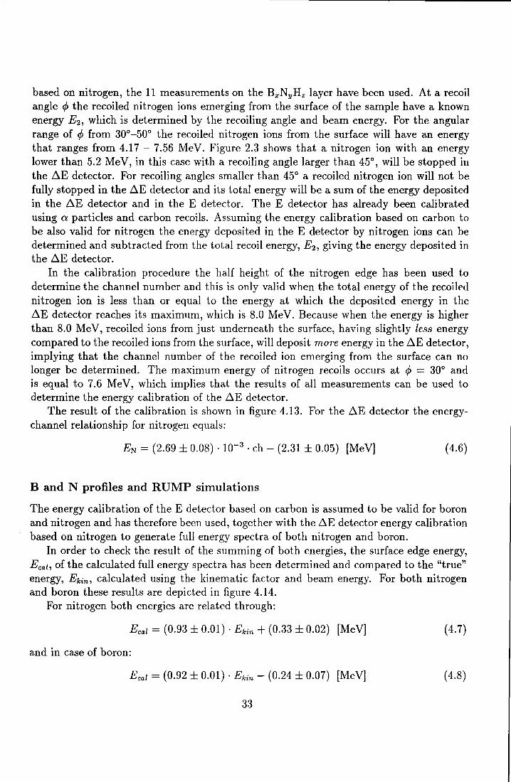
based on nitrogen, the 11 measurements on the BxNyHz layer have been used. At a recoil angle </> the recoiled nitrogen ions emerging from the surface of the sample have a known energy E 2 , which is determined by the recoiling angle and beam energy. For the angular range of </> from 30°-50° the recoiled nitrogen ions from the surface will have an energy that ranges from 4.17 - 7.56 MeV. Figure 2.3 shows that a nitrogen ion with an energy lower than 5.2 MeV, in this case with a recoiling angle larger than 45°, will be stopped in the ~E detector. For recoiling angles smaller than 45° a recoiled nitrogen ion will not be fully stopped in the ~E detector and its total energy will be a sum of the energy deposited in the ~E detector and in the E detector. The E detector has already been calibrated using a particles and carbon recoils. Assuming the energy calibration based on carbon to be also valid for nitrogen the energy deposited in the E detector by nitrogen ions can be determined and subtracted from the total recoil energy, E2 , giving the energy deposited in the ~E detector.

In the calibration procedure the half height of the nitrogen edge has been used to determine the channel number and this is only valid when the total energy of the recoiled nitrogen ion is less than or equal to the energy at which the deposited energy in the ~E detector reaches its maximum, which is 8.0 MeV. Because when the energy is higher than 8.0 Me V, recoiled ions from just underneath the surface, having slightly less energy compared to the recoiled ions from the surface, will deposit more energy in the ~E detector, implying that the channel number of the recoiled ion emerging from the surface can no longer be determined. The maximum energy of nitrogen recoils occurs at </> = 30° and is equal to 7.6 MeV, which implies that the results of all measurements can be used to determine the energy calibration of the ~E detector.

The result of the calibration is shown in figure 4.13. For the ~E detector the energy­channel relationship for nitrogen equals:

EN = (2.69 ± 0.08) · 10-3 ·eh - (2.31 ± 0.05) [MeV] (4.6)

B and N profiles and RUMP simulations

The energy calibration of the E detector based on carbon is assumed to be valid for boron and nitrogen and has therefore been used, together with the ~E detector energy calibration based on nitrogen to generate full energy spectra of both nitrogen and boron.

In order to check the result of the summing of both energies, the surface edge energy, Eca/, of the calculated full energy spectra has been determined and compared to the "true" energy, Ekin, calculated using the kinematic factor and beam energy. For both nitrogen and boron these results are depicted in figure 4.14.

For nitrogen both energies are related through:

Ecal = (0.93 ± 0.01) ·Ekin+ (0.33 ± 0.02) [MeV] (4.7)

and in case of boron:

Ecal = (0.92 ± 0.01) ·Ekin - (0.24 ± 0.07) [MeV] (4.8)

33

5.5 -~ ::!! .......... l>...5.0

~ Q)

~ ~

4.5

4·0

2400 2500 2600 2700 2800 2900 3000 3100

Channel

Figure 4.13: Energy deposited in the ~E detector by nitrogen versus the channel number.

a ......... --.--.-........., ......... -.-........ .,......,-.-........ ..,......_...--.--.-........., ......... ---.-.,......,....,

7

5

-nitrogen ······boron

.· 5

. .r

6 7 Ekin {MeV)

.. ·I"

... t

8 9

Figure 4.14: Boron and nitrogen energy according to the calibrations, EcaZ, versus nitrogen energy calculated with the kinematic factor and beam energy, Ekin·

34

Energy (MeV)

0_35

.----e ..... o __ e ..... 5 __ 1 ..... 0_.....,.....,1._5 __ e,....o__,

O.JO

¥ 0.25

~ "O 0.20

-~ "'6 0.15

E ~ 0.10

0.05

.. .. • + + +

. . .. +++++ +

+ ..... • • ........

...

0.00 ...... _.....,..__ _ __,,, _____ _,...._ .......

550 800 850 700 750 800 Channel

Energy (MeV)

0_5 ___ 5..,..5 __ e.,...o __ ...,e._5 __ 1_.0 __ 1_.5__,

"O "'ii

0.4

~ 0.3 "O Q)

-~ "'6 E 0.2 ... 0 z

0.1

0.0 p..llll.lllWL\IDlllLL:......,...--""T""---J.11..IL...J.......4 500 550 800 850 700 750

Channel

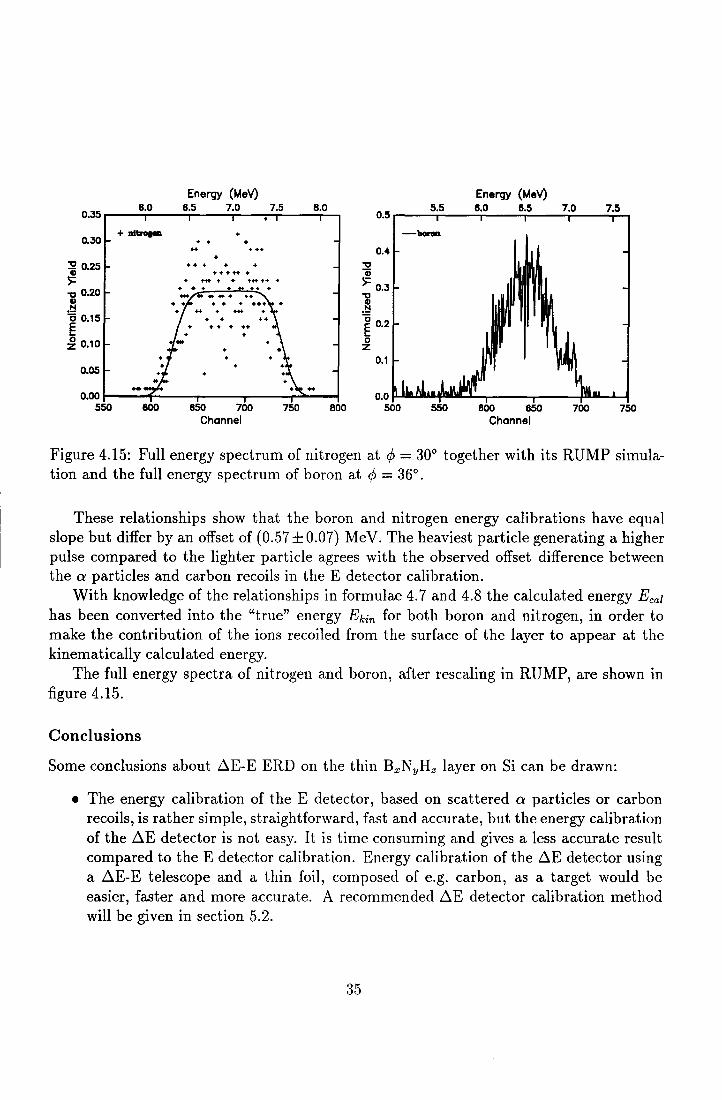
Figure 4.15: Full energy spectrum of nitrogen at <P = 30° together with its RUMP simula­tion and the full energy spectrum of boron at <P = 36°.

These relationships show that the boron and nitrogen energy calibrations have equal slope but differ by an offset of (0.57 ± 0.07) MeV. The heaviest particle generating a higher pulse compared to the lighter particle agrees with the observed offset difference between the a particles and carbon recoils in the E detector calibration.

With knowledge of the relationships in formulae 4. 7 and 4.8 the calculated energy Ecal

has been converted into the "true" energy Ekin for both boron and nitrogen, in order to make the contribution of the ions recoiled from the surface of the layer to appear at the kinematically calculated energy.

The full energy spectra of nitrogen and boron, after rescaling in RUMP, are shown in figure 4.15.

Conclusions

Some conclusions about ~E-E ERD on the thin BxNyHz layer on Si can be drawn:

• The energy calibration of the E detector, based on scattered a particles or carbon recoils, is rather simple, straightforward, fast and accnrate, but the energy calibration of the ~E detector is not easy. It is time consuming and gives a less accurate result compared to the E detector calibration. Energy calibration of the ~E detector using a ~E-E telescope and a thin foil, composed of e.g. carbon, as a target would be easier, faster and more accurate. A recommended ~E detector calibration method will be given in section 5.2.

35

5.....,...._.......,.....,.....,....., ..................................................................................... .....

']' 4 .......................................... + .......................................................... ·

§3 ..c:i ~2 -

030 32 34 36 38

rp 0

40 42 44

Figure 4.16: Angular dependence of the effective boron recoiling cross section, the dotted line is not based on a model but only added to guide the eye.

• The sample has a thickness such that the contributions of the different elements can be separated and the ~E-E telescope has proven to be a powerful tool to determine the individual depth profiles.

• The appearance of an element dependent energy calibration induces the need to generate an energy calibration for each element present in the sample in order to be able to obtain a depth profile for it.

• In the specific case of boron, depth profiling is complicated due to interplay of 10B, 11B and 10B* in the profile. However the total amount of boron (1015 at·cm-2) in the layer can be determined once the area is used an the effective boron recoiling cross section is measured.

Boron cross section

In order to be able to analyse BxCyNz layers on silicon the boron recoiling cross section has to be known. The recoiling cross section of boron recoiled by 14.6 MeV a particles for <P in the range of 30°-44° is not available in the literature and therefore the ~E-E measurements have been used to determine the angular dependence of this cross section.

The total amount of counts in the nitrogen or boron peak in the conditional E detector spectrum is proportional to both the element's concentration and recoiling cross section. According to Giorginis and Misaelides [12], who invesigated the same sample using ( a,p) reactions, the B:N ratio equals (1.016 ± 0.005):(0.984 ± 0.005). The effective boron re­coiling cross section can be obtained by comparing the total yield of boron and nitrogen. In case of boron this total yield is caused by elastically recoiled 10B and 11 B nuclei to-

36

AE detector 1000 ........ .,...,.,.....,,....,.....,..........,....,....T'""T""T""T'".......,....,.....,..........,....,....T'""T"",....,

800 c

1 800

0 u 400

200 N

0 0.._~~soo~........,~,~oooL..J..........._~,5~0~0..;c:i~2~000~~25,i-100

channel

E detector

150

50

1000 2000 3000 channel

Figure 4.17: ~E and E detector spectra of CxNyHz on Si at</>= 35°.

gether with inelastically recoiled 100 ions (Q = 0.7183 MeV). The angular dependence of the effective recoiling cross section of a natural existing 100 + 11 0 mixture is shown in figure 4.16.

4.3.3 ~E-E ERD measurements on a CxN yHz layer on Si

In order to compare the performance of ~E-E ERD for thin and thick layers a sample consisting of a thick (~1 µm) CxNyHz layer on a silicon substrate has been investigated with ~E-E ERD. The experiments have been carried out using a 14.6 MeV a particle beam because the sample contains a small amount of nitrogen and for this energy at </> = 42° the nitrogen recoiling cross section reaches a maximum.

Recoil separation with the ~E-E telescope

For the recoil angle </> = 35° the ~E and E detector spectra are given in figure 4.17. The energy deposition of carbon recoils in the ~E detector is less than that of nitrogen recoils in spite of the fact that the carbon recoils have a higher energy than the nitrogen recoils. This effect is caused by the differences in stopping power for carbon and nitrogen in analogy with the previous discussion for boron and nitrogen.

In order to be able to generate individual depth profiles for carbon and nitrogen the contributions of both elements have to be separated with the ~E-E system by generation of conditional spectra.

It is clear that the contributions of carbon and nitrogen do not appear fully separated in the ~E detector spectrum. The overlap is caused by the thickness of the investigated layer,

37

carbon nitrogen 200 30

25 150

20

!J In .... § 100 § 15 0 0 0 0

10 50

5

400 600 1000 0

100 channel

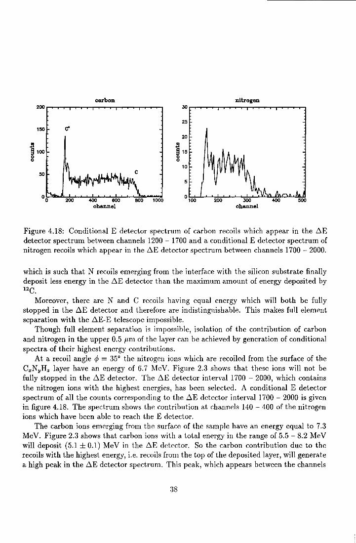
Figure 4.18: Conditional E detector spectrum of carbon recoils which appear in the ~E detector spectrum between channels 1200 - 1700 and a conditional E detector spectrum of nitrogen recoils which appear in the ~E detector spectrum between channels 1700 - 2000.

which is such that N recoils emerging from the interface with the silicon substrate finally deposit less energy in the ~E detector than the maximum amount of energy deposited by 12c.

Moreover, there are N and C recoils having equal energy which will both be fully stopped in the ~E detector and therefore are indistinguishable. This makes full element separation with the ~E-E telescope impossible.

Though full element separation is impossible, isolation of the contribution of carbon and nitrogen in the upper 0.5 µm of the layer can be achieved by generation of conditional spectra of their highest energy contributions.

At a recoil angle </> = 35° the nitrogen ions which are recoiled from the surface of the CxNyHz layer have an energy of 6.7 MeV. Figure 2.3 shows that these ions will not be fully stopped in the ~E detector. The ~E detector interval 1700 - 2000, which contains the nitrogen ions with the highest energies, has been selected. A conditional E detector spectrum of all the counts corresponding to the ~E detector interval 1700 - 2000 is given in figure 4.18. The spectrum shows the contribution at channels 140 - 400 of the nitrogen ions which have been able to reach the E detector.

The carbon ions emerging from the surface of the sample have an energy equal to 7.3 MeV. Figure 2.3 shows that carbon ions with a total energy in the range of 5.5 - 8.2 MeV will deposit (5.1±0.1) MeV in the ~E detector. So the carbon contribution due to the recoils with the highest energy, i.e. recoils from the top of the deposited layer, will generate a high peak in the ~E detector spectrum. This peak, which appears between the channels

38

+ carbon ...... ex

12

6

1500 2000 2500 Channel

3000

Figure 4.19: Energy of the scattered a particles and the recoiled carbon ions versus the channel number of the E detector spectrum.

1200 and 1700 in the ~E detector, has been selected. A conditional E detector spectrum of these selected counts is shown in figure 4.18. The contribution consists of two parts. Elastically recoiled carbon ions which deposit up to ~2.2 MeV in E detector and appear at channels lower than 800 and inelastically recoiled carbon ions (Q = 4.4391 MeV), which have an energy up to ~4.9 MeV. A small amount of them appears in the selected ~E detector spectrum interval. These inelastically recoiled carbon ions deposit ~150 keV or less in the E detector and appear at channels 140 - 200.

In case of a thick (~1 µm) CxNyHz layer on silicon the contributions of carbon and nitrogen can not be fully separated by using an incident 14.6 Me V a particle beam and applying a ~E-E telescope. Therefore a depth profile of carbon and nitrogen for the total layer can not be reconstructed, but only for the upper ~0.5 µm a depth profile can be obtained.

Energy calibration of the ~E and E detector

In order to obtain depth profiles the full energy spectrum has to be constructed. This requires the possibility to determine the the total energy of a recoiled particle. For that purpose both the ~E and E detector have been calibrated.

Assuming the beam energy to be (14.6 ± 0.2) MeV energy calibration of the E detector can be performed using scattering experiments on a thin carbon foil at the angles </> = 29.6°, 34.6°, 39.6°, 44.6°, 49.6° and 54.6°. A plot of the total energy versus the channel

39

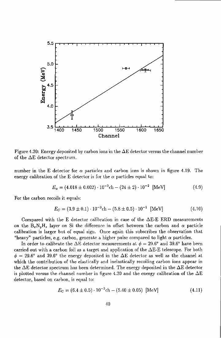
5.0

~4.5 bO J.i Q)

~ r:i::I

4.0

3·5

1400 1450 1500 1550 1600 1650

Channel

Figure 4.20: Energy deposited by carbon ions in the ~E detector versus the channel number of the ~E detector spectrum.

number in the E detector for a particles and carbon ions is shown in figure 4.19. The energy calibration of the E detector is for the a particles equal to:

Ea= (4.018 ± 0.002) · 10-3ch - (24 ± 2) · 10-2 [MeV] ( 4.9)

For the carbon recoils it equals:

Ee= (3.9 ± 0.1) · 10-3ch- (5.8 ± 0.5) · 10-1 [MeV] (4.10)

Compared with the E detector calibration in case of the ~E-E ERD measurements on the BxNyHz layer on Si the difference in offset between the carbon and a particle calibration is larger but of equal sign. Once again this subscribes the observation that "heavy" particles, e.g. carbon, generate a higher pulse compared to light a particles.

In order to calibrate the ~E detector measurements at <P = 29.6° and 39.6° have been carried out with a carbon foil as a target and application of the ~E-E telescope. For both <P = 29.6° and 39.6° the energy deposited in the ~E detector as well as the channel at which the contribution of the elastically and inelastically recoiling carbon ions appear in the ~E detector spectrum has been determined. The energy deposited in the ~E detector is plotted versus the channel number in figure 4.20 and the energy calibration of the ~E detector, based on carbon, is equal to:

Ee = (6.4 ± 0.5) · 10-3 ch - (5.40 ± 0.05) [MeV] ( 4.11)

40

8.0

-carbon .tlf 7.5 ······nitrogen

>7.0 __ ,.· Cl)

::!! .......... 6.5

i ~ 6.0

5.5

5.0 5 6 7 8 9

Ekin {MeV)

Figure 4.21: Total energy of carbon and nitrogen according to the energy calibration of the ~E and E detector, Ecal, versus the energy calculated with the kinematic factor and beam energy, Ekin.

Profiles

With the energy calibration of both ~E and E detector it is possible to reconstruct the total energy spectrum for carbon and nitrogen, which is necessary to obtain a depth profile for both elements. In order to check the energy calibrations of the ~E and E detector for carbon and nitrogen, the sum of the energy deposited in the ~E detector and in the E detector, Eca/, has been compared to the energy obtained through calculation of the kinematic factor and beam energy, Ekin· For carbon and nitrogen the results are depicted in figure 4.21.

In case of carbon the relationship equals:

Ecal = (0.87 ± 0.05) ·Ekin+ (0.5 ± 0.1) [MeV] (4.12)

and for nitrogen it is:

Ecal = (0.90 ± 0.05) ·Ekin+ (1.8 ± 0.2) [MeV] (4.13)

The difference in offset between the "heavy" nitrogen recoil and the "light" carbon recoil is similar to the previously observed offset difference in the BxNyHz on Si measurements.

The CxNyHz layer on Si has a thickness such that the recoiled carbon and nitrogen ions can not be separated fully with a ~E-E telescope with a 4.2 µm thick ~E detector. But

41

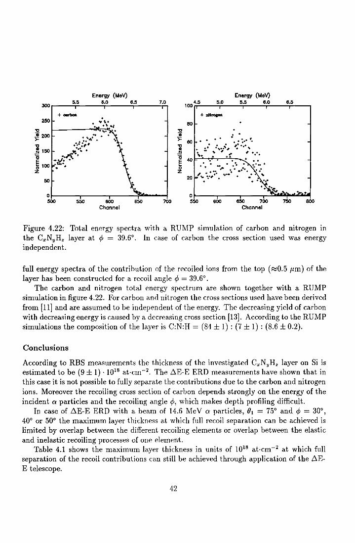
Energy (MeV) 7.0 J00.--~---.5.s,__~~-8._o~~~8-.5~~~--

250

"'C

~ 200

"'C

.~ 150 "6 E 100 0 z

50

+ OU'1lon

...... +

• .. ... + • + •••• ..•. ;.,...,. ...

~ .. ·~·· -~· .. ·'*· .. .

01--~~-.-~~~..-~~_;:;!ii!CA_.,--f

500 550 800 Channel

850 700

"'C "ii >= "'C CD . ~ "6 E ..... 0 z

Energy (MeV)

1004.5 5.0 5.5 8.0 8.5

+ Dltro&m

80

. . . . . ... ~·· "· 80 . . . . ,. .. + + . •• .. ·'\.·•"., . . '\ • .. '\ , .,. ..... '\+ .. • ..

40 . . . .. . . . . . ..... . . .. . . . .• •• + ....... . .· , + ....

20 '\i. .... ,· '\ .. ... +

0 550 800 850 700 750 800

Channel

Figure 4.22: Total energy spectra with a RUMP simulation of carbon and nitrogen in the CxNyHz layer at cp = 39.6°. In case of carbon the cross section used was energy independent.

full energy spectra of the contribution of the recoiled ions from the top ( ~0.5 µm) of the layer has been constructed for a recoil angle cp = 39.6°.

The carbon and nitrogen total energy spectrum are shown together with a RUMP simulation in figure 4.22. For carbon and nitrogen the cross sections used have been derived from [11] and are assumed to be independent of the energy. The decreasing yield of carbon with decreasing energy is caused by a decreasing cross section [13]. According to the RUMP simulations the composition of the layer is C:N:H = (84 ± 1): (7 ± 1): (8.6 ± 0.2).

Conclusions

According to RBS measurements the thickness of the investigated CxNyHz layer on Si is estimated to be (9±1) · 1018 at·cm-2

. The ~E-E ERD measurements have shown that in this case it is not possible to fully separate the contributions due to the carbon and nitrogen ions. Moreover the recoiling cross section of carbon depends strongly on the energy of the incident a particles and the recoiling angle cp, which makes depth profiling difficult.

In case of ~E-E ERD with a beam of 14.6 MeV a particles, 01 = 75° and cp = 30°, 40° or 50° the maximum layer thickness at which full recoil separation can be achieved is limited by overlap between the different recoiling elements or overlap between the elastic and inelastic recoiling processes of one element.

Table 4.1 shows the maximum layer thickness in units of 1018 at·cm-2 at which full separation of the recoil contributions can still be achieved through application of the ~E­E telescope.

42

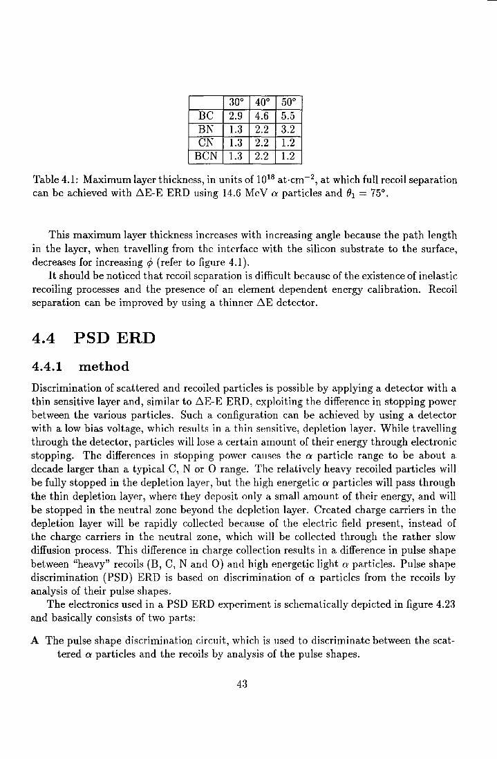
30° 40° 50° BC 2.9 4.6 5.5 BN 1.3 2.2 3.2 CN 1.3 2.2 1.2

BCN 1.3 2.2 1.2

Table 4.1: Maximum layer thickness, in units of 1018 at·cm-2 , at which full recoil separation can be achieved with ~E-E ERD using 14.6 Mc V a particles and ()1 = 75°.

This maximum layer thickness increases with increasing angle because the path length in the layer, when travelling from the interface with the silicon substrate to the surface, decreases for increasing </> (refer to figure 4.1).

It should be noticed that recoil separation is difficult because of the existence of inelastic recoiling processes and the presence of an element dependent energy calibration. Recoil separation can be improved by using a thinner ~E detector.

4.4 PSD ERD

4.4.1 method

Discrimination of scattered and recoiled particles is possible by applying a detector with a thin sensitive layer and, similar to ~E-E ERD, exploiting the difference in stopping power between the various particles. Such a configuration can be achieved by using a detector with a low bias voltage, which results in a thin sensitive, depletion layer. While travelling through the detector, particles will lose a certain amount of their energy through electronic stopping. The differences in stopping power causes the a particle range to be about a decade larger than a typical C, N or 0 range. The relatively heavy recoiled particles will be fully stopped in the depletion layer, but the high energetic a particles will pass through the thin depletion layer, where they deposit only a small amount of their energy, and will be stopped in the neutral zone beyond the depletion layer. Created charge carriers in the depletion layer will be rapidly collected because of the electric field present, instead of the charge carriers in the neutral zone, which will be collected through the rather slow diffusion process. This difference in charge collection results in a difference in pulse shape between "heavy" recoils (B, C, N and 0) and high energetic light a particles. Pulse shape discrimination (PSD) ERD is based on discrimination of a particles from the recoils by analysis of their pulse shapes.

The electronics used in a PSD ERD experiment is schematically depicted in figure 4.23 and basically consists of two parts:

A The pulse shape discrimination circuit, which is used to discriminate between the scat­tered a particles and the recoils by analysis of the pulse shapes.

43

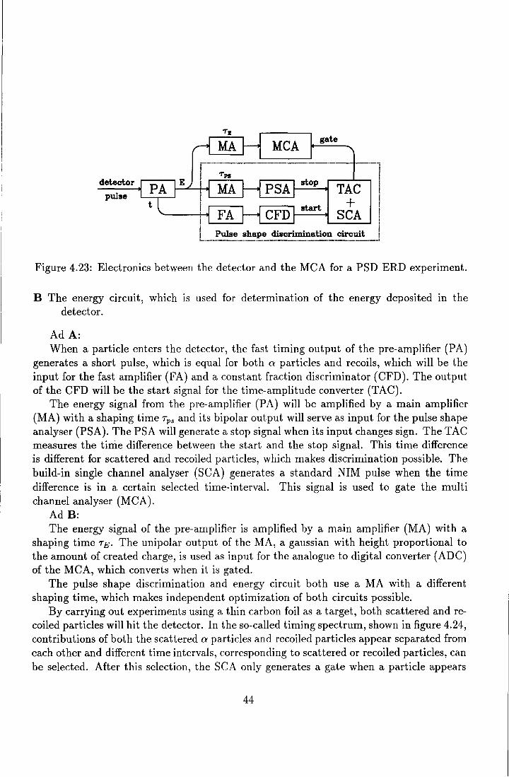
T1

MA MCA gate

r··-·· .. ···~:--·--·--·--·--·--·--·--·--·--·--·--· detector .--P-A----.i-E"""'-­

pulse t

MA

FA

....---'-----. PSA

stop

start CFD--

TAC +

SCA Pulse shape discrimination circuit

Figure 4.23: Electronics between the detector and the MCA for a PSD ERD experiment.

B The energy circuit, which is used for determination of the energy deposited in the detector.

Ad A: When a particle enters the detector, the fast timing output of the pre-amplifier (PA)

generates a short pulse, which is equal for both a particles and recoils, which will be the input for the fast amplifier (FA) and a constant fraction discriminator (CFD). The output of the CFD will be the start signal for the time-amplitude converter (TAC).

The energy signal from the pre-amplifier (PA) will be amplified by a main amplifier (MA) with a shaping time Tps and its bipolar output will serve as input for the pulse shape analyser (PSA). The PSA will generate a stop signal when its input changes sign. The TAC measures the time difference between the start and the stop signal. This time difference is different for scattered and recoiled particles, which makes discrimination possible. The build-in single channel analyser (SCA) generates a standard NIM pulse when the time difference is in a certain selected time-interval. This signal is used to gate the multi channel analyser (MCA).

AdB: The energy signal of the pre-amplifier is amplified by a main amplifier (MA) with a

shaping time TE. The unipolar output of the MA, a gaussian with height proportional to the amount of created charge, is used as input for the analogue to digital converter (ADC) of the MCA, which converts when it is gated.

The pulse shape discrimination and energy circuit both use a MA with a different shaping time, which makes independent optimization of both circuits possible.

By carrying out experiments using a thin carbon foil as a target, both scattered and re­coiled particles will hit the detector. In the so-called timing spectrum, shown in figure 4.24, contributions of both the scattered a particles and recoiled particles appear separated from each other and different time intervals, corresponding to scattered or recoiled particles, can be selected. After this selection, the SCA only generates a gate when a particle appears

44

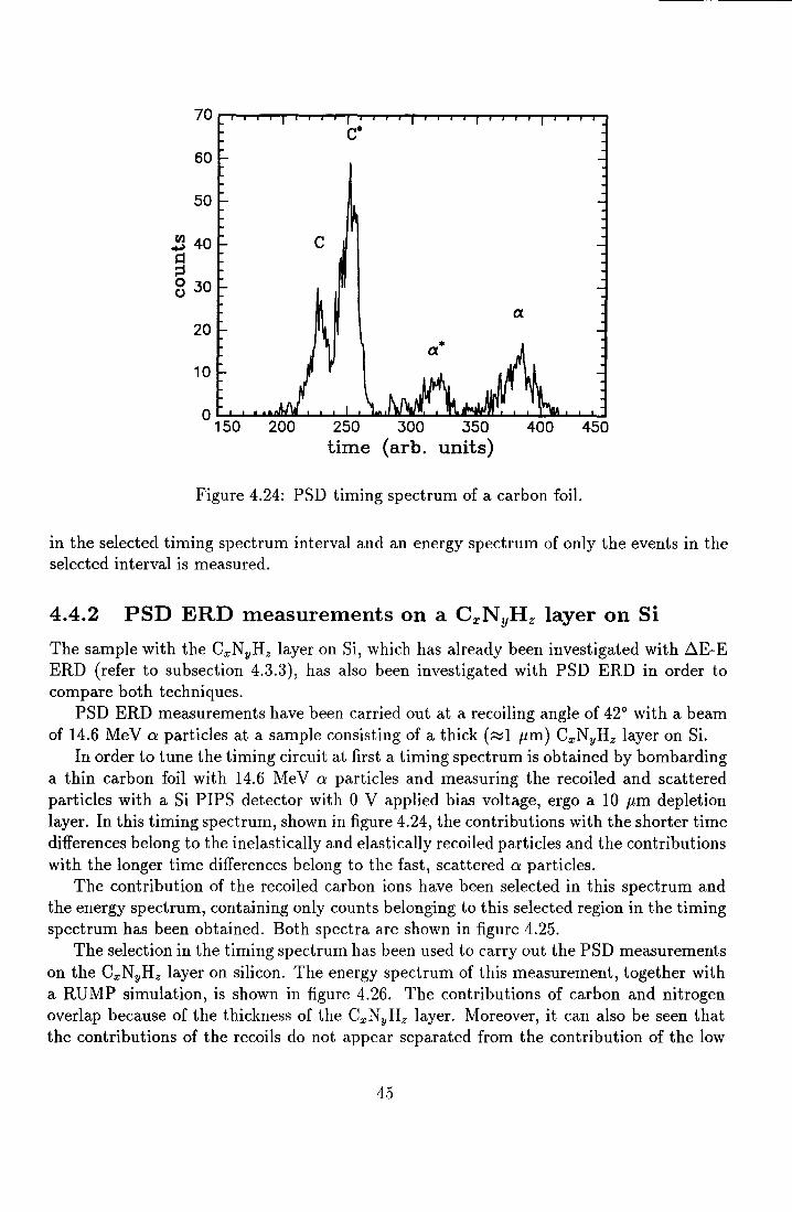
70 c·

60

50

.!1 40 c ~ ::s 0 30 0

20

10

0150 200 250 300 350 400 450

time (arb. units)

Figure 4.24: PSD timing spectrum of a carbon foil.

in the selected timing spectrum interval and an energy spectrum of only the events in the selected interval is measured.

4.4.2 PSD ERD measurements on a CxN yHz layer on Si

The sample with the CxNyHz layer on Si, which has already been investigated with ~E-E ERD (refer to subsection 4.3.3), has also been investigated with PSD ERD in order to compare both techniques.

PSD ERD measurements have been carried out at a recoiling angle of 42° with a beam of 14.6 MeV a particles at a sample consisting of a thick (~1 µm) CxNyHz layer on Si.

In order to tune the timing circuit at first a timing spectrum is obtained by bombarding a thin carbon foil with 14.6 MeV a particles and measuring the recoiled and scattered particles with a Si PIPS detector with 0 V applied bias voltage, ergo a 10 µm depletion layer. In this timing spectrum, shown in figure 4.24, the contributions with the shorter time differences belong to the inelastically and elastically recoiled particles and the contributions with the longer time differences belong to the fast, scattered a particles.

The contribution of the recoiled carbon ions have been selected in this spectrum and the energy spectrum, containing only counts belonging to this selected region in the timing spectrum has been obtained. Both spectra are shown in figure 4.25.

The selection in the timing spectrum has been used to carry out the PSD measurements on the CxNyHz layer on silicon. The energy spectrum of this measurement, together with a RUMP simulation, is shown in figure 4.26. The contributions of carbon and nitrogen overlap because of the thickness of the CxNyHz layer. Moreover, it can also be seen that the contributions of the recoils do not appear separated from the contribution of the low

45

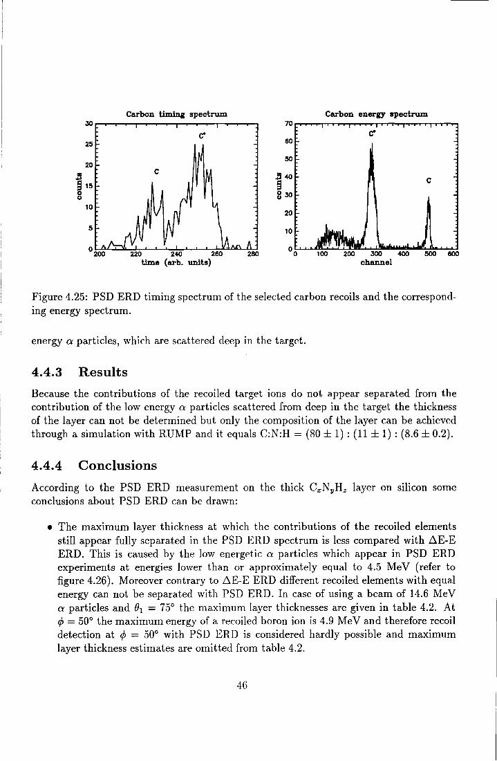
Carbon tiining spectru.In 30 ......... ---.-......... .......-....-........ ---.---.--..-.......-........., ........... --.

25

20

!l ~ 15 g

10

5

Carbon energy spectru.In 70 ........ ...,..,...,....,....,....,....,....,.. ........ ...,..,...,....,....,....,....,....,..,........,...,..,.....,...,.. .....

60

50

c

20

10

100 200 300 400 500 600 channel

Figure 4.25: PSD ERD timing spectrum of the selected carbon recoils and the correspond­ing energy spectrum.

energy a particles, which are scattered deep in the target.

4.4.3 Results

Because the contributions of the recoiled target ions do not appear separated from the contribution of the low energy a particles scattered from deep in the target the thickness of the layer can not be determined but only the composition of the layer can be achieved through a simulation with RUMP and it equals C:N:H = (80 ± 1) : (11 ± 1) : (8.6 ± 0.2).

4.4.4 Conclusions

According to the PSD ERD measurement on the thick CxNyHz layer on silicon some conclusions about PSD ERD can be drawn:

• The maximum layer thickness at which the contributions of the recoiled elements still appear fully separated in the PSD ERD spectrum is less compared with ~E-E ERD. This is caused by the low energetic a particles which appear in PSD ERD experiments at energies lower than or approximately equal to 4.5 MeV (refer to figure 4.26). Moreover contrary to ~E-E ERD different recoiled elements with equal energy can not be separated with PSD ERD. In case of using a beam of 14.6 MeV a particles and ()1 = 75° the maximum layer thicknesses are given in table 4.2. At </> = 50° the maximum energy of a recoiled boron ion is 4.9 Me V and therefore recoil detection at </> = 50° with PSD ERD is considered hardly possible and maximum layer thickness estimates are omitted from table 4.2.

46

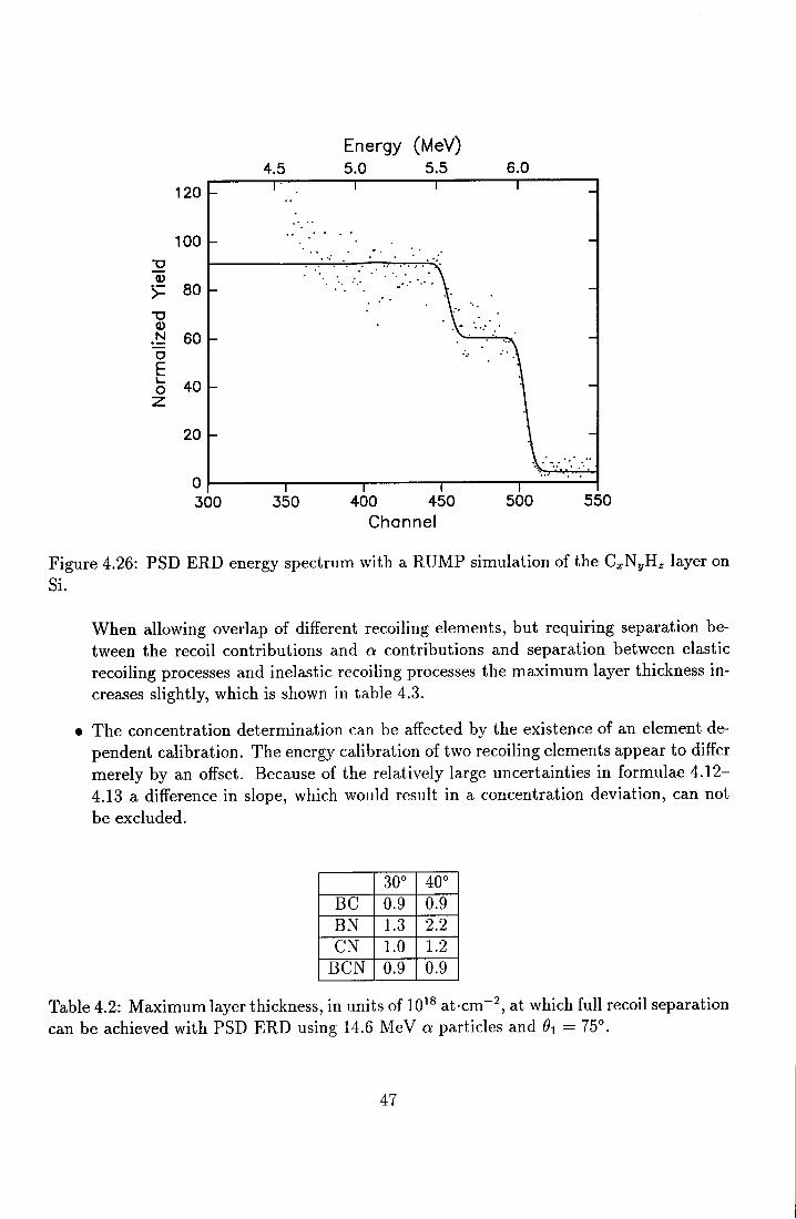
4.5

120

100 "O Q)

>= 80

"O Q) N 60 ·-0 E L.. 40 0 z

20

0 300 350

Energy (MeV) 5.0 5.5

.... ..... . . .. . ·. •,• .·

.·

400 450 Channel

6.0

500

.. . . ·

550

Figure 4.26: PSD ERD energy spectrum with a RUMP simulation of the CxNyHz layer on Si.

When allowing overlap of different recoiling elements, but requiring separation be­tween the recoil contributions and a contributions and separation between elastic recoiling processes and inelastic recoiling processes the maximum layer thickness in­creases slightly, which is shown in table 4.3.

• The concentration determination can be affected by the existence of an element de­pendent calibration. The energy calibration of two recoiling elements appear to differ merely by an offset. Because of the relatively large uncertainties in formulae 4.12-4.13 a difference in slope, which would result in a concentration deviation, can not be excluded.

30° 40° BC 0.9 0.9 BN 1.3 2.2 CN 1.0 1.2

BCN 0.9 0.9

Table 4.2: Maximum layer thickness, in units of 1018 at·cm-2, at which full recoil separation

can be achieved with PSD ERD using 14.6 MeV a particles and 01 = 75°.

47

30° 40° BC 2.9 4.6 BN 1.3 2.2 CN 1.3 2.2

BCN 1.3 2.2

Table 4.3: Maximum layer thickness, in units of 1018 at·cm-2 , at which depth profiling with PSD ERD using 14.6 MeV a particles and 01 = 75° is still possible.

• The discrimination of recoils from the scattered particles is based on selection of the recoil contribution in the timing spectrum of a carbon foil. This selected interval does not necessarily have to correspond with the interval at which the recoiled elements from the thick layer appear because:

- elements of interest other than carbon are present in the layer. These elements need not generate a pulse equal to that of carbon.

- carbon recoils from the thick layer may have energies such that they appear outside the selected interval in the timing spectrum.

4.5 ~E-E ERD versus PSD ERD

According to the ~E-E ERD measurements the composition of the layer equals C:N:H = (84 ± 1) : (7 ± 1) : (8.6 ± 0.2) though in case of PSD ERD the composition is found to be equal to C:N:H = (80 ± 1): (11±1): (8.6 ± 0.2).

The results of the ~E-E ERD and PSD ERD measurements are, with respect to the composition, not equal and this difference can be caused by various effects:

Cross section deviation caused by:

• deviation of the beam energy. A difference of 100 ke V might already cause the carbon recoiling cross section to deviate ::::::40%,

• deviation of the recoil angle caused by (refer to figure 4.27):

- the beam of projectiles entering the scattering chamber with an angular deviation De,

- misplacement of the detector by D</>,

A total misplacement D</> + De ::::::: 1° might result in the carbon recoiling cross section to differ ::::::20%.

Different energy calibration for different recoiling elements which might cause the en­ergy width of one channel to be different for different recoils. The RUMP code

48

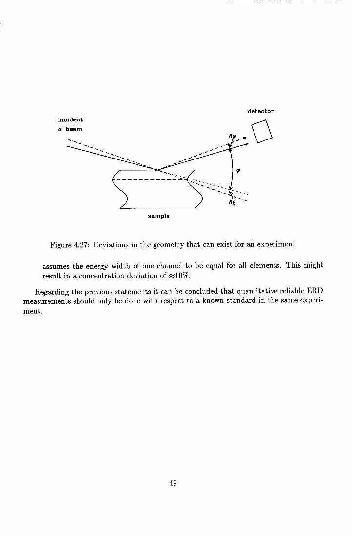
incident

a beam

sample

detector

0

Figure 4.27: Deviations in the geometry that can exist for an experiment.

assumes the energy width of one channel to be equal for all elements. This might result in a concentration deviation of ~10%.

Regarding the previous statements it can be concluded that quantitative reliable ERD measurements should only be done with respect to a known standard in the same experi­ment.

49

Chapter 5

ERDA WITH a PARTICLES FOR MATERIALS ANALYSIS conclusions and recommendations

In this chapter the performance of the two different configurations used to carry out ERD experiments with a particles are evaluated. 6-E-E ERD and PSD ERD methods are com­pared and in addition conclusions which hold for both techniques are drawn. Finally this chapter ends with recommendations for further investigation.

5.1 Conclusions

In chapter 4 ERD experiments are described and 6-E-E ERD and PSD ERD will be compared with respect to their capabilities in depth profiling and determination of the absolute amount of atoms·cm-2 of a certain element present in a layer on a silicon substrate using a beam of 14.6 MeV a particles, 01 = 75° and </> = 30°, 40° or 50°.

Highest accuracy in measurement of the composition and absolute amount of atoms·cm-2

in a layer is achieved when the contributions of the recoiled elements can be separated fully from each other, the contribution of the a particles and from the contribution of their own inelastic processes. This full separation can be achieved up to a maximum layer thickness which is different for both methods. In case of 6-E-E ERD the maximum thicknesses are given in table 5.1. In case of PSD ERD the maximum thicknesses are lower compared to 6-E-E ERD and given in table 5.2. The ability with 6-E-E ERD to separate the contribu­tions of recoiled ions through generation of conditional spectra causes the maximum layer thicknesses to be larger compared to PSD ERD.

When full recoil separation is possible the accuracy of the determined total amount of atoms·cm-2 present of a certain element is limited by the accuracy of the absolute cross section, which is :::::10%. Determination of the concentration ratio of two elements in a layer, which is proportional to the ratio of their recoiling cross section, can be done with higher accuracy for the relative recoiling cross sections when using a beam of 14.6 MeV a

50

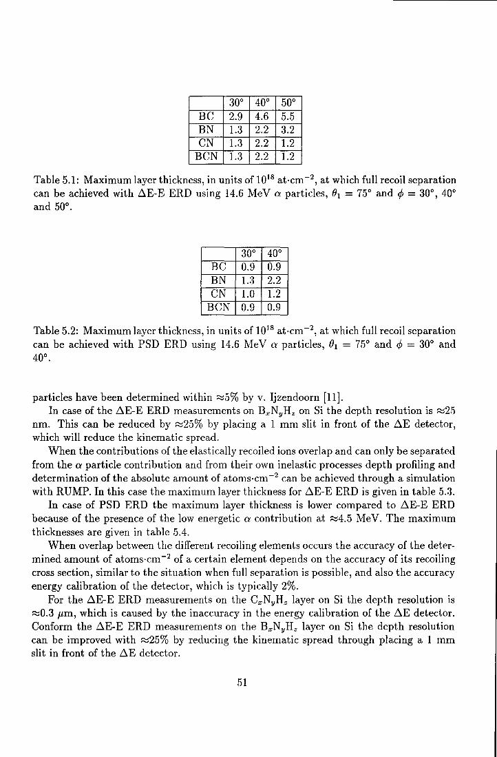
30° 40° 50° BC 2.9 4.6 5.5 BN 1.3 2.2 3.2 CN 1.3 2.2 1.2

BCN 1.3 2.2 1.2

Table 5.1: Maximum layer thickness, in units of 1018 at·cm-2 , at which full recoil separation can be achieved with ~E-E ERD using 14.6 MeV a particles, 81 = 75° and</>= 30°, 40° and 50°.

30° 40° BC 0.9 0.9 BN 1.3 2.2 CN 1.0 1.2

BCN 0.9 0.9

Table 5.2: Maximum layer thickness, in units of 1018 at·cm-2 , at which full recoil separation can be achieved with PSD ERD using 14.6 MeV a particles, 81 = 75° and </> = 30° and 40°.

particles have been determined within ~5% by v. ljzendoorn [11]. In case of the ~E-E ERD measurements on BxNyHz on Si the depth resolution is ~25

nm. This can be reduced by ~25% by placing a 1 mm slit in front of the ~E detector, which will reduce the kinematic spread.

When the contributions of the elastically recoiled ions overlap and can only be separated from the a particle contribution and from their own inelastic processes depth profiling and determination of the absolute amount of atoms·cm-2 can be achieved through a simulation with RUMP. In this case the maximum layer thickness for ~E-E ERD is given in table 5.3.

In case of PSD ERD the maximum layer thickness is lower compared to ~E-E ERD because of the presence of the low energetic a contribution at ~4.5 MeV. The maximum thicknesses are given in table 5.4.

When overlap between the different recoiling elements occurs the accuracy of the deter­mined amount of atoms·cm-2 of a certain element depends on the accuracy of its recoiling cross section, similar to the situation when full separation is possible, and also the accuracy energy calibration of the detector, which is typically 2%.

For the ~E-E ERD measurements on the CxNyHz layer on Si the depth resolution is ~0.3 µm, which is caused by the inaccuracy in the energy calibration of the ~E detector. Conform the ~E-E ERD measurements on the BxNyIIz layer on Si the depth resolution can be improved with ~25% by reducing the kinematic spread through placing a 1 mm slit in front of the ~E detector.

51

30° 40° 50° BC 2.9 4.6 5.5 BN 1.3 2.2 3.2 CN 1.3 2.2 3.2

BCN 1.3 2.2 3.2

Table 5.3: Maximum layer thickness, in units of 1018 at·cm-2, at which depth profiles can still be obtained with ~E-E ERD using 14.6 MeV a particles, 01 = 75° and </> = 30°, 40° and 50°.

30° 40° BC 2.9 4.6 BN 1.3 2.2 CN 1.3 2.2

BCN 1.3 2.2

Table 5.4: Maximum layer thickness, in units of 1018 at·cm-2 , at which depth profiles can be still obtained with PSD ERD using 14.6 MeV a particles and 01 = 75° and</>= 30° and 40°.

During the PSD ERD measurements on the CxNyHz layer on Si a 1 mm slit has been present in front of the Si PIPS detector. In this case the depth resolution is ~100 nm and significantly better than the depth resolution achieved with the ~E-E measurements on the same sample.

Apart from depth resolution and determination of the composition of a layer other differences between ~E-E ERD and PSD ERD exist:

• The PSD ERD measurements are difficult to reproduce contrary to the ~E-E mea­surements. This is caused by the discrimination based on timing being very sensitive to minor changes of the parameters set via the electronical circuit.

• In case of PSD ERD the total energy spectrum is on-line visible, contrary to ~E­E ERD. This means that during a PSD ERD experiment it is easier to determine whether the measurement provides the expected spectrum. The absence of on-line visibility of the ~E-E ERD total energy spectrum is caused by the limitations of the present software which does not support total energy spectrum display.

• In case of PSD ERD it could be possible that the selection of recoiled particles in the timing spectrum, based on scattering on a thin foil, does not cover all particles recoiled from a thicker layer on a silicon substrate. The energy spectrum obtained

52

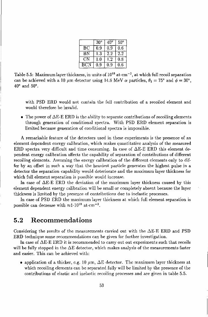
30° 40° 50° BC 0.9 0.9 0.6 BN 1.3 2.2 2.2 CN 1.0 1.2 0.8

BCN 0.9 0.9 0.6

Table 5.5: Maximum layer thickness, in units of 1018 at·cm-2 , at which full recoil separation can be achieved with a 10 µm detector using 14.6 MeV a particles, 01 = 75° and </> = 30°, 40° and 50°.

with PSD ERD would not contain the full contribution of a recoiled element and would therefore be invalid.

• The power of ~E-E ERD is the ability to separate contributions of recoiling elements through generation of conditional spectra. With PSD ERD element separation is limited because generation of conditional spectra is impossible.

A remarkable feature of the detectors used in these experiments is the presence of an element dependent energy calibration, which makes quantitative analysis of the measured ERD spectra very difficult and time consuming. In case of ~E-E ERD this element de­pendent energy calibration affects the capability of separation of contributions of different recoiling elements. Assuming the energy calibration of the different elements only to dif­fer by an offset in such a way that the heaviest particle generates the highest pulse in a detector the separation capability would deteriorate and the maximum layer thickness for which full element separation is possible would increase.

In case of ~E-E ERD the deviation of the maximum layer thickness caused by this element dependent energy calibration will be small or completely absent because the layer thickness is limited by the presence of contributions due to inelastic processes.

In case of PSD ERD the maximum layer thickness at which full element separation is possible can decrease with ~1·1018 at·cm-2 .

5.2 Recommendations

Considering the results of the measurements carried out with the ~E-E ERD and PSD ERD technique some recommendations can be given for further investigation.

In case of ~E-E ERD it is recommended to carry out out experiments such that recoils will be fully stopped in the ~E detector, which makes analysis of the measurements faster and easier. This can be achieved with:

• application of a thicker, e.g. 10 µm, ~E detector. The maximum layer thickness at which recoiling elements can be separated fully will be limited by the presence of the contributions of elastic and inelastic recoiling processes and are given in table 5.5.

53

60° BC 0.6 BN 1.8 CN 0.9

BCN 0.6

Table 5.6: Maximum layer thickness, in units of 1018 at·cm-2 , at which full element separa­tion can still be achieved with a ~E-E ERD detector using 14.6 MeV a particles, (Ji = 75° and </> = 60°.

30° BC 0.1 BN 0.5 CN 0.2

BCN 0.1

Table 5. 7: Maximum layer thickness, in units of 1018 at·cm-2 , at which full element sepa­ration can still be achieved with a ~E-E ERD detector using 5 Me V a particles, 01 = 75° and </> = 30°.

• measuring at larger recoiling angles. A huge asset is the energies of the inelastic recoiling of 11 B, 12 C or 14N being lower than or equal to ~1.5 Me V when </> ~ 60°. But the energy of the recoils decreases and a drawback is the decreasing maximum layer thickness at which the recoil contributions can be separated from each other. For the case of using a 14.6 MeV a particle beam, 01 = 75° and</>= 60° the maximum layer thicknesses are given in table 5.6.

• measuring with lower beam energies. Full stopping of boron, carbon and nitrogen at </> = 30° can be achieved by using a beam of 5 Me V a particles. At these low energies the maximum layer thickness at which the contributions of the different recoiling elements still appear separate from each other decreases dramatically, which can be seen in table 5. 7.

Of all possibilities the application of a 10 µm ~E detector is the best. Compared to the current ~E-E telescope the maximum layer thickness at which full recoil contribution separation can be achieved will deteriorate slightly, but the depth resolution will improve ~30% because the detection system consists of only one detector and therefore one detec­tor resolution. Moreover the analysis of the measured data will be less time consuming compared to the analysis of the currently obtained data.

54

For both ~E-E ERD and PSD ERD the following recommendations can be given:

• The maximum BxCyNz layer thickness at which full separation of the contributions of the recoiling elements can be achieved depends on the composition of the layer as has been discussed in section 5.1. Regarding full recoiling element contribution separation as the most ideal situation using samples with deposited layers of thickness less than the maximum thickness is highly recommended.

• The existence of an element dependent detector response makes detector energy cal­ibration for each individual element necessary for proper depth profiling. An energy calibration for element A can be performed by carrying out scattering experiments on a thin foil containing element A and measuring at different angles </> as discussed in subsection 4.3.2 and 4.3.3.

In case of using a ~E-E telescope and a beam of 14.6 MeV a particles the ~E detector can be calibrated for carbon and nitrogen by carrying out scattering experiments on a thin foil and measuring with the ~E-E telescope at different recoiling angles </>.

The following procedures can be used:

- In case of carbon measurements at </> = 38°, 44° and 48° have to be carried out. The energies deposited by the inelastically recoiled carbon ions will be respectively 2.1, 3.0 and 4.3 MeV. At </> = 38° the elastically recoiled carbon ions will deposit ~5.1 MeV in the ~E detector, so with three fast and easy measurements four points for the energy calibration will be obtained. A higher accuracy can be obtained by measuring at more angles between 38° and 48°.

- In case of nitrogen measurements at </> = 45°, 50° and 55° have to be carried out. The energies deposited by the elastically recoiled nitrogen ions will be respec­tively 5.05, 4.17 and 3.32 Me V and the energies deposited by the inelastically recoiled nitrogen ions will be respectively 3.95, 3.06 and 2.17 MeV. At these angles all nitrogen ions will stop and the energy calibration will not depend on the energy calibration of the E detector. With three measurements 6 points for the energy calibration will be obtained. A higher accuracy can be obtained by measuring at more angles between 45° and 55°.

55

Bibliography

[1] W.K. Chu, J.W. Mayer and M.A. Nicolet Backscattering Spectrometry Academic Press (1978)

[2] L.C. Feldman and J.W. Mayer Fundamentals on Surface and Thin Film Analysis Elsevier Science Publishing B.V., The Netherlands (1986)

[3] Glenn F. Knoll Radiation detection and measurement Wiley (1989)

[4] J. F. Ziegler, J. P. Biersack, and U. Littmark The stopping and range of ions in solids, Volume 1 Pergamon Press (1985)

[5] J. F. Ziegler Helium Stopping Powers and Ranges in All Elements, Volume 4 Pergamon Press (1977)

[6] H.A. Rijken Detection methods for depth profiling of light elements using high energy alpha

particles PhD Thesis, Eindhoven University of Technology (1993)

[7] W.M. Arnold Bik Elastic Recoil Detection and Hydrogen Chemistry in Silicon Oxynitrides Faculteit Natuur- en Sterrenkunde, Rijksuniversiteit te Utrecht (1992)

56

[8] Lawrence R. Doolittle Algorithms for the rapid simulation of Rutherford backscattering spectra Nuclear Instruments and Methods B9, p344 (1985)

[9] Lawrence R. Doolittle High Energy Backscattering Analysis Using RUMP Conference Proceedings, Heavy Ion Beams. Materials Research Society (1990)

(10] Michael Bozoian Deviations from Rutherford backscattering for Z = 1, 2 projectiles Nuclear Instruments and Methods B58, p.127 - 131 (1991)

[11] L.J. van ljzendoorn, H.A. Rijken, S.S. Klein and M.J.A. de Voigt Elastic Recoil Detection of Light elements (C,N,0} with high energy

{10 - 15 Me VJ He beams Applied Surface Science 70/71, p.58 (1993)

(12] G. Giorginis and P. Misaelides Characterization of boron nitride thin films using (a,p} nuclear reactions ECAART Conference proceedings (1993), to be published.

(13] Carter, Mitchell and Davis Elastic Scattering of Alpha Particles by c1 2 in the Bombarding Energy Range 10 to 19 MeV Phys. Rev. 133, p. 1421 (1964)

[14] Mitchell, Carter and Davis Inelastic Scattering of 6- to 19-1\fe V Alpha Particles from Carbon* Phys. Rev. 133, p. 1434 (1964)

[15] P.W.L. van Dijk Analysis of Light Elements in Thin Films using High Energy Ion Scattering Techniques Master of Science Thesis, Eindhoven University of Technology (1992)

(16] Jeroen Jonkers Multi Parameter Ion Scattering Techniques Master of Science Thesis, Eindhoven University of Technology (1993)

[17] E. Dekempeneer Private communications

57

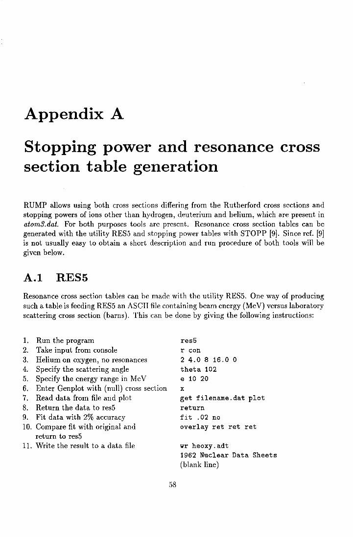
Appendix A

Stopping power and resonance cross section table generation

RUMP allows using both cross sections differing from the Rutherford cross sections and stopping powers of ions other than hydrogen, deuterium and helium, which are present in atom3.dat. For both purposes tools are present. Resonance cross section tables can be generated with the utility RESS and stopping power tables with STOPP [9). Since ref. [9) is not usually easy to obtain a short description and run procedure of both tools will be given below.

A.1 RES5

Resonance cross section tables can be made with the utility RESS. One way of producing such a table is feeding RESS an ASCII file containing beam energy (Me V) versus laboratory scattering cross section (barns). This can be done by giving the following instructions:

1. Run the program 2. Take input from console 3. Helium on oxygen, no resonances 4. Specify the scattering angle S. Specify the energy range in Me V 6. Enter Genplot with (null) cross section 7. Read data from file and plot 8. Return the data to resS 9. Fit data with 2% accuracy 10. Compare fit with original and

return to resS 11. Write the result to a data file

S8

res5 r con 2 4.0 8 16.0 0 theta 102 e 10 20 x get filename.dat plot return fit .02 no overlay ret ret ret

wr heoxy.adt 1962 Nuclear Data Sheets (blank line)

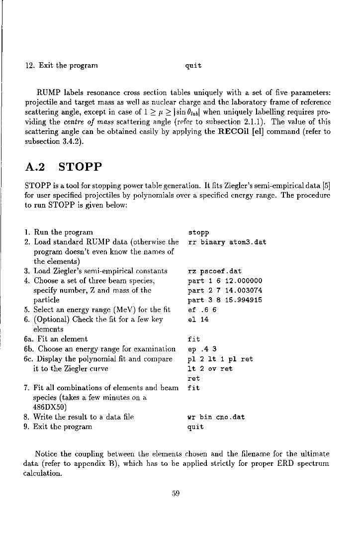
12. Exit the program quit

RUMP labels resonance cross section tables uniquely with a set of five parameters: projectile and target mass as well as nuclear charge and the laboratory frame of reference scattering angle, except in case of 1 ~ µ ~ I sin 01abl when uniquely labelling requires pro­viding the centre of mass scattering angle (refer to subsection 2.1.1). The value of this scattering angle can be obtained easily by applying the RECOil [el] command (refer to subsection 3.4.2).

A.2 STOPP STOPP is a tool for stopping power table generation. It fits Ziegler's semi-empirical data [5] for user specified projectiles by polynomials over a specified energy range. The procedure to run STOPP is given below:

1. Run the program 2. Load standard RUMP data (otherwise the

program doesn't even know the names of the elements)

3. Load Ziegler's semi-empirical constants 4. Choose a set of three beam species,

specify number, Z and mass of the particle

5. Select an energy range (Me V) for the fit 6. (Optional) Check the fit for a few key

elements 6a. Fit an element 6b. Choose an energy range for examination 6c. Display the polynomial fit and compare

it to the Ziegler curve

7. Fit all combinations of elements and beam species (takes a few minutes on a 486DX50)

8. Write the result to a data file 9. Exit the program

stopp rr binary atorn3.dat

rz pscoef.dat part 1 6 12.000000 part 2 7 14.003074 part 3 8 15.994915 ef .6 6 el 14

fit ep .4 3 pl 2 lt 1 pl ret lt 2 ov ret ret fit

wr bin cno.dat quit

Notice the coupling between the elements chosen and the filename for the ultimate data (refer to appendix B), which has to be applied strictly for proper ERD spectrum calculation.

59

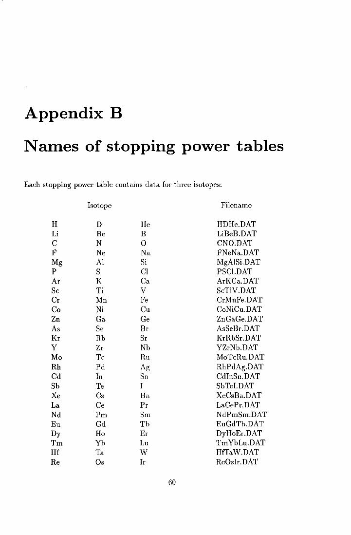
Appendix B

Names of stopping power tables

Each stopping power table contains data for three isotopes:

Isotope Filename

H D He HDHe.DAT Li Be B LiBeB.DAT c N 0 ONO.DAT F Ne Na FNeNa.DAT Mg Al Si MgAlSi.DAT p s Cl PSCl.DAT Ar K Ca ArKCa.DAT Sc Ti v ScTiV.DAT Cr Mn Fe CrMnFe.DAT Co Ni Cu CoNiCu.DAT Zn Ga Ge ZnGaGe.DAT As Se Br AsSeBr.DAT Kr Rb Sr KrRbSr.DAT y Zr Nb YZrNb.DAT Mo Tc Ru MoTcRu.DAT Rh Pd Ag RhPdAg.DAT Cd In Sn CdlnSn.DAT Sb Te I Sb Tel.DAT Xe Cs Ba XeCsBa.DAT La Ce Pr LaCePr.DAT Nd Pm Sm NdPmSm.DAT Eu Gd Tb EuGdTb.DAT Dy Ho Er DyHoEr.DAT Tm Yb Lu TmYbLu.DAT Hf Ta w HfTaW.DAT Re Os lr ReOslr.DAT

60

Pt Au Hg PtAuHg.DAT TI Pb Bi TIPbBi.DAT Po At Rn PoAtRn.DAT Fr Ra Ac FrRaAc.DAT Th Pa u ThPaU.DAT

61

Appendix C

Rutherford recoiling cross section

The cross section for elastic recoiling can easily be derived from the centre of mass Ruther­ford scattering cross section. The amount of particles recoiling in a certain solid angle df2rec equals the amount of scattered particles in the corresponding solid angle df2scat:

[ d ] lab [ d l c.m. d~ ( <P1ab) sin <fa1abd<fatab = d~ ( Bc.m.) sin Bc.m.dBc.m.

rec scat The relationship

leads to

ergo

and

0 c.m. = 7r - 2<fa1ab

sin Oc.m. = 2 sin <P1ab cos <P1ab

dOc.m. = _ 2 d<fatab

. (Oc.m.) sm -2- = cos <P1ab

(C.l)

(C.2)

(C.3)

(C.4)

(C.5)

The centre of mass energy is related to the laboratory frame of reference energy through

µ+l Etab = Ecm-­

µ

The centre of mass Rutherford scattering cross section equals:

(C.6)

[ da ( Bc.m.)] c.m. = ( Z1 Z2e2 ) 2 1 [m. sr-1] (C. 7) df! scat 167rt:oEc.m. sin4

( ~)

Substition of formulae C.3- C. 7 into formula C. l leads to the laboratory frame of reference Rutherford recoiling cross section given in formula 2.4

62

Appendix D

Rutherford scattering cross section

In case of an elastic binary collision the centre of mass frame of reference Rutherford scattering cross section is given by:

[dO" (() )] c.m. = ( Z1Z2e

2 )

2 _1_

df! c.m. scat l 67rloEc.m. sin 4 ( fJc..t·) [m · sr-1

] (D.l)

The laboratorium frame of reference Rutherford scattering cross sections can easily be derived by application of basic highschool mathematics.

In the centre of mass frame of reference the amount of scattered particles in a cer­tain solid angle d!1~~7:i equals in the amount of scattered particles in the corresponding laboratory frame of reference solid angle df!~~~t:

[d l c.m. [d l lab d~(Oc.m.) sinOc.m.dOc.m. = d~(()lab) sin01abd01ab

scat scat

(D.2)

Transformation of the centre of mass frame of reference scattering cross section into the laboratory frame of reference scattering cross section merely requires the analytic re­lationship between ()lab and Oc.m. which is given by [2]:

() µsin Oc.m. tan lab = ----­

µCOS Oc.m. + 1

From formula D.3 cos Oc.m. can simply be derived:

() _ sin201ab COS ()lab V 2 • 2 ()

cos c.m. - - ± µ - sm lab µ µ

(D.3)

(D.4)

With this relationship the ratio of the differential scattering cross sections can easily be determined to be:

sin () c.m. d() c.m.

sin 01abd{}zab

( J1i2 - sin201ab ± cos 01ab)

2

µJ µ 2 - sin201ab

63

(D.5)

The centre of mass frame of reference scattering cross section contains the centre of mass scattering angle Oc.m.· Basic goniometry shows that

• 4 (Oc.m.) = (1- cosOc.m.)2

sm 2 2 (D.6)

Combination of the previous formulae lead to the following expression for the laboratory frame of reference scattering cross section [m·sr-1]:

(D.7)

The case with the higher of the ± and =f leads to the cross section belonging to the event with a kinematic factor given by formula 2.1. The other case leads to the scattering cross section belonging to the event with a kinematic factor given by formula 2.2

In case of events with a kinematic factor equal to formula 2.1 the laboratorium frame of reference scattering cross section can be simplified, which leads to the famous Rutherford cross section [m·sr-1]:

[du ] lab an (()lab)

scat

(D.8)

The cases with a kinematic factor given in formula 2.2 have a slightly different cross section [m·sr-1]:

64