eigen series solutions to terminal-state tracking optimal control problems and exact controllability...

a

y

in thistributedigenmatenishesd whichulae.

xact

J. Math. Anal. Appl. 313 (2006) 284–310

www.elsevier.com/locate/jma

Eigen series solutions to terminal-state trackingoptimal control problems and exact controllabilit

problems constrained by linear parabolic PDEs

L. Steven Houa, Oleg Imanuvilova, Hee-Dae Kwonb,∗,1

a Department of Mathematics, Iowa State University, Ames, IA 50011, USAb Department of Mathematics, Inha University, Incheon 402-751, South Korea

Received 4 December 2003

Available online 18 July 2005

Submitted by M.D. Gunzburger

Abstract

Terminal-state tracking optimal control problems for linear parabolic equations are studiedpaper. The control objectives are to track a desired terminal state and the control is of the distype. Explicit solution formulae for the optimal control problems are derived in the form of eseries. Pointwise-in-timeL2 norm estimates for the optimal solutions are obtained and approxicontrollability results are established. Exact controllability is shown when the target state vaon the boundary of the spatial domain. One-dimensional computational results are presenteillustrate the terminal-state tracking properties for the solutions expressed by the series form 2005 Elsevier Inc. All rights reserved.

Keywords:Terminal-state tracking; Optimal control; Parabolic equations; Eigen series; Approximate and econtrollability

* Corresponding author.E-mail addresses:[email protected] (L.S. Hou), [email protected] (O. Imanuvilov),

[email protected] (H.-D. Kwon).1 The research of this author was supported by Inha University Research Grant (INHA-32742).

0022-247X/$ – see front matter 2005 Elsevier Inc. All rights reserved.doi:10.1016/j.jmaa.2005.02.067

L.S. Hou et al. / J. Math. Anal. Appl. 313 (2006) 284–310 285

inearterval

ttudy

olic

t as-ptimalbility

int

ments

iond thee of

1. Introduction

In this paper we study terminal-state tracking optimal control problems for a lsecond order parabolic partial differential equation (PDE) defined over the time in[0, T ] ⊂ [0,∞) and on a bounded,C2 (or convex) spatial domainΩ ⊂ R

d , d = 1, 2 or 3.Let a target functionW ∈ L2(Ω) and an initial conditionw ∈ L2(Ω) be given and lef ∈ L2((0, T )×Ω) denote the distributed control. The optimal control problems we sare to minimize the terminal-state tracking functional

J (u,f ) = T

2

∫Ω

∣∣u(T ,x) − W(x)∣∣2 dx + γ

2

T∫0

∫Ω

∣∣f (t,x)∣∣2 dxdt (1.1)

or

K(u,f ) = T

2

∫Ω

∣∣u(T ,x) − W(x)∣∣2 dx + γ

2

T∫0

∫Ω

∣∣f (t,x) − F(t,x)∣∣2 dxdt (1.2)

(whereγ is a positive constant andF is a given reference function) subject to the parabPDE

ut − div[A(x)∇u

] = f, (t,x) ∈ (0, T ) × Ω, (1.3)

with the homogeneous boundary condition

u = 0, (t,x) ∈ (0, T ) × ∂Ω, (1.4)

and the initial condition

u(0,x) = w(x), x ∈ Ω. (1.5)

In (1.3), A(x) is a symmetric matrix-valued,C1(Ω) function that is uniformly positivedefinite.

Similar optimal control problems have been studied in the literature from differenpects or in different settings. For instance, in [15] the existence and regularity of an osolution was studied; in [2] the connection between optimal solutions and controllawas examined, and in [22] eigen series solutions were studied wherein the controlf wasassumed to belong to a bounded set inL2((0, T ) × Ω) (due to the boundedness constrathe tracking functional of [22] did not contain the term involvingf ). Both optimal controlproblems and controllability problems are studied in this paper. Our main achieveconcerning optimal control problems include: the introduction of anF in (1.2) that re-sults in an optimal solution that approaches the target more effectively (even fort T

and moderate parameterγ ); the derivation and justification of explicit eigen series solutformulae for optimal solutions; pointwise-in-time estimates for optimal solutions anapproximately controllability properties for the optimal solutions. A distinctive featurthis work is that the desired terminal-stateW and the admissible stateu are allowed tohave nonmatching boundary conditions, though the reference functionF need be suitablychosen in the formulation of cost functional (1.2) (the details about the choice ofF will berevealed in Section 2).

286 L.S. Hou et al. / J. Math. Anal. Appl. 313 (2006) 284–310

Theystud-value

neralweakprox-nd thehen

lemsertainl func-ntroltions

thetargetustrateulae of

ace

thodonsve

Terminal-state tracking problems are optimal control problems in their own right.are also closely related to approximate and exact controllability problems which wereied in, among others, [1–5,7–14,17–20]. As mentioned in the foregoing the boundaryfor the target stateW may be nonzero so that the parabolic problem (1.3)–(1.5) in geis not exactly controllable when the solution for (1.3)–(1.5) is defined in the standardsense (see [6]). Contributions of this paper on controllability consist of the proof of apimate controllability when the target state has an inhomogeneous boundary value aderivation of explicit series solution formulae for the exact controllability problem wthe target state vanishes on the boundary.

In Section 2 we formulate the optimal control problems and controllability probin an appropriate mathematical framework. In Section 3 we review and establish cresults concerning eigen functions expansions for both spatial and temporal–spatiations. In Section 4 we derive explicit eigen series solution formulae for the optimal coproblems. In Section 5 we derive pointwise-in-time estimates for the optimal soluand show that as the parameterγ → 0, the optimal solutions at the terminal timeT ap-proach the target stateW . In Section 6 we justify eigen series solution formulae forexact controllability problem by assuming homogeneous boundary values for thestate. In Section 7 we present some one-dimensional computational results that illthe terminal-state tracking properties for the solutions expressed by the series formSection 4.

2. Formulation of optimal control and controllability problems

Throughout we freely make use of standard Sobolev space notationsHm(Ω) andH 1

0 (Ω). We denote the norm for Sobolev spaceHm(Ω) by ‖ · ‖m. Note thatH 0(Ω) =L2(Ω) so that‖ · ‖0 is theL2(Ω) norm. We will need the temporal–spatial function sp

H 2,1((0, T ) × Ω) =

v ∈ L2(0, T ;H 2(Ω)): vt ∈ L2(0, T ;L2(Ω)

).

A temporal–spatial functionv(t,x) often will be simply written asv(t).Functional (1.1) can be written as

J (u,f ) = T

2

∥∥u(T ) − W∥∥2

0 + γ

2

T∫0

∥∥f (t)∥∥2

0 dt. (2.1)

Regarding functional (1.2) the idea for constructing the reference functionF is that wefirst choose a reference functionU(t,x) satisfyingU(T ,x) = W (i.e., U is a given paththat reachesW at timeT ) and then set

F = Ut − div[A(x)∇U

]in [0, T ] × Ω.

However,W (and thusU ) in general does not vanish on the boundary. The series meto be studied in this paper will involve eigen series expressions for reference functiF

andU . The validity of these expressions requireU to vanish on the boundary. To resolthis difficulty we choose the reference functionF = F (γ ) (which is dependent ofγ ) as fol-


eady-fornce

weak

-

lows. We first choose a one-parameter set of functionsW(γ ): γ > 0 ⊂ H 2(Ω) ∩ H 10 (Ω)

such that∥∥W(γ ) − W∥∥

0 → 0 asγ → 0. (2.2)

(If W ∈ H 2(Ω)∩H 10 (Ω), then we may simply chooseW(γ ) = W that is independent ofγ .

In general,W has an inhomogeneous boundary condition andW(γ ) approximatesW in theL2(Ω) sense.) Next, for each givenγ > 0, we choose a functionV (γ )(t,x) that satisfies

V (γ ) ∈ L2(0, T ;H 2(Ω) ∩ H 10 (Ω)

), V

(γ )t ∈ L2(0, T ;L2(Ω)

),

V (γ )(T ) = W(γ ) in Ω; (2.3)

in other words,V (γ ) is an arbitrarily chosen smooth path that reachesW(γ ) at timeT . Byvirtue of (2.2)–(2.3) we have∥∥V (γ )(T ) − W

∥∥0 → 0 asγ → 0. (2.4)

We also assume∥∥V (γ )(0)∥∥

0 C whereC > 0 is a constant independent ofγ . (2.5)

The choices of aV (γ ) that satisfies (2.3)–(2.5) are certainly nonvacuous, e.g., the ststate functionV (γ )(t, ·) = W(γ ) is a particular and convenient choice. Here we allowmore general choices of such a pathV (γ )(t, ·) than the steady-state one. The referefunctionF is now defined by

F = F (γ ) ≡ V(γ )t − div

[A(x)∇V (γ )

]in (0, T ) × Ω. (2.6)

Functional (1.2) may be written

K(u,f ) = T

2

∥∥u(T ) − W∥∥2

0 + γ

2

T∫0

∥∥f (t) − F(t)∥∥2

0 dt

= T

2

∥∥u(T ) − W∥∥2

0 + γ

2

T∫0

∥∥∥∥f (t) − d

dtV (γ )(t) − div

[A(x)∇V (γ )(t)

]∥∥∥∥2

0dt.

(2.7)

The solution to the constraint equations (1.3)–(1.5) is understood in the followingsense.

Definition 2.1. Let f ∈ L2((0, T );L2(Ω)) andw ∈ L2(Ω) be given.u is said to be a solution of (1.3)–(1.5) ifu ∈ L2((0, T );H 1

0 (Ω)), ut ∈ L2((0, T );H−1(Ω)), andu satisfies⟨ut (t), φ

⟩ + ∫Ω

[A(x)∇u(t)

] · ∇φ dx = ⟨f (t),φ

⟩ ∀φ ∈ H 10 (Ω), a.e.t ∈ (0, T ),

u(0) = w in Ω, (2.8)

where〈·,·〉 denotes the duality pairing betweenH−1(Ω) andH 10 (Ω).


from

e

ility.

f

Remark. A weak solution in the sense of Definition 2.1 belongs toC([0, T ];L2(Ω)),see [6].

An admissible element for the optimal control problem is a pair(u,f ) that satisfies theinitial boundary value problem (2.8). The precise definition is given as follow.

Definition 2.2. Let w ∈ L2(Ω) be given. A pair(u,f ) is said to be anadmissible ele-ment if u ∈ L2((0, T );H 1

0 (Ω)), ut ∈ L2((0, T );H−1(Ω)), f ∈ L2((0, T );L2(Ω)), and(u,f ) satisfies Eq. (2.8). The set of all admissible elements is denoted byVad((0, T ),w)

or simplyVad.

The optimal control problems we study can be concisely stated as:

(OP1) seek a pair(u, f ) ∈ Vad such thatJ (u, f ) = inf(u,f )∈VadJ (u,f ) where the func-tionalJ is defined by (2.1);

and

(OP2) seek a pair(u, f ) ∈ Vad such thatK(u, f ) = inf(u,f )∈VadK(u,f ) where the func-tionalK is defined by (2.7).

The existence and uniqueness of optimal solutions for (OP1) and (OP2) followclassical optimal control theories (see, e.g., [15]):

Theorem 2.3. Assume thatw ∈ L2(Ω) and W ∈ L2(Ω). Then there exists a uniqusolution (u, f ) ∈ Vad to (OP1) and to (OP2). If, in addition, w ∈ H 1

0 (Ω), then u ∈H 2,1((0, T ) × Ω).

The approximate and exact controllability problems are formulated as follows:

(AP-CON) seek a one-parameter set(uε, fε): ε > 0 ⊂ Vad such that

limε→0

∥∥uε(T ) − W∥∥

0 = 0

and

(EX-CON) seek a pair(u,f ) ∈ Vad such that

u(T ) = W in Ω.

Of course, exact controllability, whenever it holds, implies approximate controllabIn particular, ifw andW belong toH 1

0 (Ω), then the exact controllability holds.

Theorem 2.4. Assume thatw ∈ H 10 (Ω). Then(EX-CON) has a solution if and only i

W ∈ H 1(Ω).
0


o-

2.3,

t

Theundary

termsr con-igen

Proof. If (EX-CON) has a solution(u,f ), then regularity for parabolic PDEs [6, Therem 5, p. 360; Theorem 4, p. 288] impliesu ∈ H 2,1(Q) andu ∈ C([0, T ];H 1(Ω)) so thatW = u(T ) ∈ H 1(Ω). Sinceu = 0 on(0, T ) × ∂Ω , we have that

‖W‖1/2,∂Ω = limt→T −

∥∥u(T ) − u(t)∥∥

1/2,∂Ω C lim

t→T −∥∥u(T ) − u(t)

∥∥1 = 0,

where‖ · ‖1/2,∂Ω denotes the norm for the Sobolev spaceH 1/2(∂Ω). Thus,W ∈ H 10 (Ω).

Conversely, assume thatW ∈ H 10 (Ω). Let u be a function satisfying

u ∈ H 2,1((0, T ) × Ω), u = 0 on(0, T ) × ∂Ω, u|t=0 = w ∈ H 1

0 (Ω).

The existence of such au is guaranteed by the trace theorem [16, vol. II, Theoremp. 18] or by the existence and regularity results (see [6]) for the parabolic problem

ut − u = 0 in (0, T ) × Ω, u = 0 in (0, T ) × ∂Ω, u|t=0 = w.

Likewise, there exists au satisfying

˜u ∈ H 2,1((0, T ) × Ω), ˜u = 0 on(0, T ) × ∂Ω, ˜u|t=T = W ∈ H 1

0 (Ω).

We choose a functionθ = θ(t) ∈ C∞[0, T ] such that

θ(t) = 1 ∀t ∈ [0, T /3] and θ(t) = 0 ∀t ∈ [2T/3, T ],and setu = θ(t)u + [1− θ(t)] ˜u in (0, T ) × Ω . Clearly,

u ∈ H 2,1((0, T ) × Ω), u = 0 on(0, T ) × ∂Ω,

u|t=0 = w, u|t=T = W.

By definingf ≡ ut − div[A(x)∇u] ∈ L2((0, T ) × Ω) we see that(u,f ) solves the exaccontrollability problem (EX-CON). Remark. The exact controllability result of [2, Theorem 3.7] was stated imprecisely.proof of that theorem, in fact, required the target state to have the homogeneous bocondition.

3. Results concerning eigen function expansions

The main objective of this paper is to find explicit solution formulae, expressed inof eigen-function expansions, for optimal control problems (OP1) and (OP2) and fotrollability problem (EX-CON). In this section we will review some properties for the epairs and eigen function expansions.

We recall the following lemma (see [6, Theorem 1, p. 335]).

Lemma 3.1. The setΛ of all eigen values for the elliptic operator−div(A(x)∇) may bewrittenΛ = λi∞i=1 ⊂ R where

0< λ1 λ2 λ3 · · · and λi → ∞ asi → ∞.


.

337].step 3,

ns of

-

s 2

Furthermore, there exists a set of corresponding eigen functionsei∞i=1 ⊂ H 2(Ω) ∩H 1

0 (Ω) which forms an orthonormal basis ofL2(Ω) (with respect to theL2(Ω) innerproduct).

In the sequel we let(λi, ei)∞i=1 denote a set of eigen pairs as stated in Lemma 3.1

Lemma 3.2. The setei/√

λi∞i=1 forms an orthonormal basis ofH 10 (Ω) with respect to

the inner product

(u, v) → B[u,v] ≡∫Ω

A(x)∇u · ∇v dx ∀u,v ∈ H 10 (Ω). (3.1)

The setei/λi∞i=1 forms an orthonormal basis ofH 2(Ω) ∩ H 10 (Ω) with respect to the

inner product

(u, v) → B[u,v] ≡∫Ω

div[A(x)∇u

]div

[A(x)∇v

]dx ∀u,v ∈ H 2(Ω) ∩ H 1

0 (Ω).

(3.2)

Proof. The first statement of this lemma is proved in [6, Theorem 1, p. 335; step 3, p.The proof for the second statement is a verbatim repetition of [6, Theorem 1, p. 335;p. 337] with the inner productB[·,·] replaced byB[·,·] (defined in (3.2)).

Based on Lemmas 3.1 and 3.2 we may establish the following characterizatioH 1

0 (Ω).

Lemma 3.3. Assumey ∈ L2(Ω) andy = ∑∞i=1 yiei in L2(Ω). Then the following state

ments are equivalent:

(i) y ∈ H 10 (Ω);

(ii) y = ∑∞i=1 yiei in H 1

0 (Ω);(iii)

∑∞i=1 λi |yi |2 < ∞.

Proof. We first prove (i) implies (ii). But this follows from [6, Theorem 1, p. 335; stepand 3, p. 337].

We next prove (ii) implies (iii). Assumey = ∑∞i=1 yiei in H 1

0 (Ω). By Lemma 3.2 wemay writey = ∑∞

i=1 yiei/√

λi in H 10 (Ω) and

∑∞i=1 |yi |2 = B[y, y] < ∞. Comparingy =∑∞

i=1 yiei/√

λi andy = ∑∞i=1 yiei in L2(Ω) we obtainyi = √

λiyi so that∑∞

i=1 λi |yi |2 =∑∞i=1 |yi |2 < ∞.Finally, we prove (iii) implies (i). Assume that

∑∞i=1 λi |yi |2 < ∞. We note that the

definition of the eigen pairs implies

B[ei, v] = λi

∫eiv dx ∀v ∈ H 1

0 (Ω)

Ω


-

-term

so thatB[ei, ej ] = 0 if j = i andB[ei, ei] = λi . Thus,

B

[n+p∑i=n

yiei,

n+p∑j=n

yj ej

]=

n+p∑i=n

λi |yi |2

so that∑ni=1 yiei∞n=1 ⊂ H 1

0 (Ω) is a Cauchy sequence with respect to theH 10 (Ω) norm

induced by theB[·,·] inner product. Hence∑∞

i=1 yiei = y in H 10 (Ω) for somey ∈ H 1

0 (Ω).But y = ∑∞

i=1 yiei in L2(Ω) and we concludey = y ∈ H 10 (Ω).

Similar arguments yield the following characterizations ofH 2(Ω) ∩ H 10 (Ω).

Lemma 3.4. Assumey ∈ L2(Ω) andy = ∑∞i=1 yiei in L2(Ω). Then the following state

ments are equivalent:

(i) y ∈ H 2(Ω) ∩ H 10 (Ω);

(ii) y = ∑∞i=1 yiei in H 2(Ω) ∩ H 1

0 (Ω);(iii)

∑∞i=1 |λi |2|yi |2 < ∞.

The main results of this section are the two theorems below concerning term-bydifferentiations of eigen series for functions inH 2,1((0, T )×Ω)∩C([0, T ];H 1

0 (Ω)). Wefirst quote a lemma (see [21, Lemma 1.1, p. 169] and [6, Theorem 2, p. 286]):

Lemma 3.5. Assumeu ∈ L2(0, T ;L2(Ω)) andut ∈ L2(0, T ;L2(Ω)). Then

−T∫

0

φ′(t)∫Ω

u(t)v dxdt =T∫

0

φ(t)

∫Ω

ut (t)v dxdt ∀φ ∈ C∞0 (0, T ), ∀v ∈ L2(Ω).

Theorem 3.6. Assume thatu ∈ H 2,1((0, T ) × Ω), u = 0 on (0, T ) × ∂Ω and

u(t) =∞∑i=1

ui(t)ei in L2(Ω), a.e.t ∈ (0, T ).

Then

∞∑i=1

T∫0

(∣∣u′i (t)

∣∣2 + |λi |2∣∣ui(t)

∣∣2)dt = ‖ut‖2L2(0,T ;L2(Ω))

+T∫

0

B[u,u]dt < ∞, (3.3)

∞∑i=1

|λi |∣∣ui(0)

∣∣2 dt < ∞, (3.4)

ut (t) =∞∑

u′i (t)ei in L2(Ω), a.e.t ∈ (0, T ) (3.5)

i=1


and

−div[A(x)∇u(t)

] =∞∑i=1

λiui(t)ei in L2(Ω), a.e.t. (3.6)

Proof. We first note the continuous embeddingH 2,1((0, T ) × Ω) → C([0, T ];H 1(Ω))

and the boundary conditionu = 0 on (0, T ) × ∂Ω imply that u(t) ∈ H 10 (Ω) for every

t ∈ [0, T ]. By Lemma 3.3 we have

u(t) =∞∑i=1

ui(t)ei in H 10 (Ω),∀t ∈ [0, T ].

In particular, sinceu(0) ∈ H 10 (Ω), Lemma 3.3 yields (3.4).

Using theL2(Ω) orthonormality ofei we have

‖u‖2L2(0,T ;L2(Ω))

=T∫

0

∥∥u(t)∥∥2

0 dt =T∫

0

∞∑i=1

∣∣ui(t)∣∣2 dt

T∫0

∣∣uj (t)∣∣2 dt ∀j

so that eachuj ∈ L2(0, T ). Sinceut ∈ L2(0, T ;L2(Ω)), we may write

ut (t) =∞∑i=1

vi(t)ei in L2(Ω), a.e.t

and

‖ut‖2L2(0,T ;L2(Ω))

=T∫

0

∥∥ut (t)∥∥2

0 dt =T∫

0

∞∑i=1

∣∣vi(t)∣∣2 dt

T∫0

∣∣vj (t)∣∣2 dt ∀j (3.7)

so that eachvj ∈ L2(0, T ). Using Lemma 3.5 we have that

−T∫

0

φ′(t)∫Ω

u(t)ej dxdt =T∫

0

φ(t)

∫Ω

ut (t)ej dxdt

∀φ ∈ C∞0 (0, T ), j = 1,2, . . . .

Substituting series expressions foru andut into the last equation and using theL2(Ω)

orthonormality ofei we obtain

−T∫

0

φ′(t)uj (t) dt =T∫

0

φ(t)vj (t) dt ∀φ ∈ C∞0 (0, T ), j = 1,2, . . . ,

so thatvj = u′j for j = 1,2, . . . . This proves (3.5).

Sinceu(t) ∈ H 2(Ω) ∩ H 10 (Ω) for almost everyt , Lemma 3.4 implies that

u(t) =∞∑

ui(t)ei in H 2(Ω) ∩ H 10 (Ω), a.e.t

i=1


arrive

-

so that

−div[A(x)∇u(t)

] =∞∑i=1

−div[A(x)∇ui(t)ei

] =∞∑i=1

λiui(t)ei in L2(Ω), a.e.t,

i.e., (3.6) holds.From (3.6) we obtain

T∫0

B[u,u]dt =T∫

0

∥∥div[A(x)∇u(t)

]∥∥20 dt =

T∫0

∞∑i=1

|λi |2∣∣ui(t)

∣∣2 dt. (3.8)

Adding up (3.7) and (3.8) and applying the Monotone Convergence theorem weat (3.3). Theorem 3.7. Assume that the set of functionsui(t)∞i=1 ⊂ H 1(0, T ) satisfies

∞∑i=1

T∫0

(∣∣u′i (t)

∣∣2 + |λi |2∣∣ui(t)

∣∣2)dt < ∞ (3.9)

and∞∑i=1

|λi |∣∣ui(0)

∣∣2 dt < ∞. (3.10)

Then the functionu formally defined byu(t) = ∑∞i=1 ui(t)ei satisfies

u ∈ H 2,1((0, T ) × Ω), u = 0 on (0, T ) × ∂Ω,

ut (t) =∞∑i=1

u′i (t)ei in L2(Ω), a.e.t, (3.11)

and

−div[A(x)∇u(t)

] =∞∑i=1


Proof. We note that

∞∑i=1

T∫0

∣∣ui(t)∣∣2 dt 1

|λ1|2∞∑i=1

T∫0

|λi |2∣∣ui(t)

∣∣2 dt < ∞

so thatu(t) = ∑∞i=1 ui(t)ei in L2(Ω) for almost everyt ∈ (0, T ).

By assumption (3.9) we are justified to definef ∈ L2((0, T );L2(Ω)) as the series function

f =∞∑

fi(t)ei ≡∞∑[

u′i (t) + λiui(t)

]ei in L2(Ω), a.e.t ∈ (0, T ).

i=1 i=1


as a.)

It is well known thatH 1(0, T ) is continuously embedded intoC[0, T ] so thatui(0)

is well defined for eachi. Assumption (3.10) and Lemma 3.3 imply thatu|t=0 ∈ H 10 (Ω)

whereu|t=0 = ∑∞i=1 ui(0)ei .

Let u be the solution for the parabolic problem

ut − div[A(x)∇u

] = f in (0, T ) × Ω, u = 0 on(0, T ) × ∂Ω,

u|t=0 = u|t=0 (3.13)

in the sense of Definition 2.1. Regularity for parabolic PDEs impliesu ∈ H 2,1((0, T )×Ω).We writeu = ∑∞

i=1 ui (t)ei in L2(Ω) for almost everyt ∈ (0, T ). Employing Theorem 3.6we have

ut (t) =∞∑i=1

u′i (t)ei in L2(Ω), a.e.t (3.14)

and

−div[A(x)∇u(t)

] =∞∑i=1


Thus, we may write (3.13) in the series form∑∞i=1

[u′

i (t) + λiui(t)]ei = ∑∞

i=1 fi(t)ei in L2(Ω), a.e.t,∑∞i=1 ui (0) = ∑∞

i=1 ui(0)ei in L2(Ω)

so that for eachi,

ui (t) + λiui(t) = fi(t) in (0, T ), ui(0) = ui(0). (3.16)

From the definition offi we see that eachui satisfies the same equations asui . The unique-ness of the solution for the initial value problem (3.16) impliesui ≡ ui in (0, T ) for eachiso thatu(t) = u(t) in L2(Ω) for everyt . Hence,u = u ∈ H 2,1((0, T ) × Ω) andu = u = 0on (0, T ) × ∂Ω). Also, Eqs. (3.14) and (3.15) yield (3.11) and (3.12).

4. Solutions of the optimal control problems

We express all functions involved asL2(Ω)-convergent series ofei:

u(t,x) =∞∑i=1

ui(t)ei(x), f (t,x) =∞∑i=1

fi(t)ei(x), w(x) =∞∑i=1

wiei(x),

W(x) =∞∑i=1

Wiei(x), V (γ )(t,x) =∞∑i=1

V(γ )

i (t)ei(x).

We work out below an explicit formula for the optimal solution of (OP1) expressedseries of eigen functionsei. (For the existence of optimal solutions, see Theorem 2.3


-

Theorem 4.1. Assumew ∈ H 10 (Ω) and W ∈ L2(Ω). Let (u, f ) ∈ H 2,1((0, T ) × Ω) ×

L2((0, T ) × Ω) be the solution of(OP1). Then

u(t,x) =∞∑i=1

ui (t)ei(x), (4.1)

where

ui (t) = wi

(e−λi t − T e−λiT (eλi t − e−λi t )

2λiγ eλiT + T (eλiT − e−λiT )

)+ Wi

T (eλi t − e−λi t )

2λiγ eλiT + T (eλiT − e−λiT ). (4.2)

Proof. Let (u,f ) be an arbitrary admissible element, thenu ∈ H 2,1((0, T ) × Ω) ∩C([0, T ];H 1

0 (Ω)). We may writeu = ∑∞i=1 ui(t)ei andf = ∑∞

i=1 fi(t)ei in L2(Ω) foralmost everyt . Moreover, Theorem 3.6 implies

ut =∞∑i=1

u′i (t)ei in L2(Ω), a.e.t

and

−div[A(x)∇u

] =∞∑i=1

λiui(t)ei in L2(Ω), a.e.t.

Thus we may rewrite the constraint equations (2.8) as∫Ω

(∑∞j=1

[u′

j (t) + λjuj (t)]ej

)ei dx = ∫

Ω

(∑∞j=1 fj (t)ej

)ei dx, i = 1,2, . . . ,∫

Ω

(∑∞j=1 uj (0)ej

)ei = ∫

Ω

(∑∞j=1 wjej

)ei dx, i = 1,2, . . . ,

so that for eachi,

u′i (t) + λiui(t) = fi(t) in (0, T ), ui(0) = wi. (4.3)

The functionalJ also can be written in the series form

J (u,f ) = T

2

∞∑i=1

∣∣ui(T ) − Wi

∣∣2 + γ

2

∞∑i=1

T∫0

∣∣fi(t)∣∣2 dt. (4.4)

The optimal control problem (OP1) is recast into:

(OP1) minimize functional (4.4) subject to the constraints (4.3) for alli = 1,2, . . . .

Since the constraint equations are fully uncoupled for eachi, the optimal control problem ( ˜OP1) is equivalent to:

(OP1i ) for eachi = 1,2, . . . , minimizeJi (ui, fi) subject to the constraints (4.3),


y

i-

6).

with

ulaP1)

where the functionalJi (ui, fi) is defined by

Ji (ui, fi) = T

2

∣∣ui(T ) − Wi

∣∣2 + γ

2

T∫0

∣∣fi(t)∣∣2 dt.

The pair(u, f ) = (∑∞

i=1 ui (t)ei(x),∑∞

i=1 fi (t)ei(x)) is the solution for (OP1) if and onlif (ui , fi ) is the solution for(OP1i ) for everyi.

To solve the constrained minimization problem (˜OP1i ) we introduce a Lagrange multplier ξi and form the Lagrangian

Li (ui, fi, ξi) = T

2

∣∣ui(T ) − Wi

∣∣2 − ui(T )ξi(T ) + wiξi(0)

+T∫

0

(γ

2

∣∣fi(t)∣∣2 + ui(t)ξ

′i (t) − λiui(t)ξi(t) + fi(t)ξi(t)

)dt.

By taking variations of the Lagrangian with respect toξi , ui andfi , respectively, we obtainan optimality system which consists of (4.3),

ξ ′i (t) − λiξi(t) = 0 in (0, T ), ξi(T ) = T

(ui(T ) − Wi

)(4.5)

and

ξi(t) = −γfi(t) . (4.6)

We proceed to solve for(ui , fi) from the optimality system formed by (4.3), (4.5) and (4.By eliminatingξi from (4.5)–(4.6) we have

f ′i (t) − λifi(t) = 0 in (0, T ), fi(T ) = −T

γ

(ui(T ) − Wi

). (4.7)

Combining (4.7) and (4.3) we arrive at a second order ordinary differential equationinitial and terminal conditions:

u′′i (t) − λ2

i ui(t) = 0 in (0, T ),

ui(0) = wi,

u′i (T ) + λiui(T ) = −T

γ

(ui(T ) − Wi

).

(4.8)

The general solution to this differential equation is

ui(t) = C1e−λi t + C2e

λi t .

The initial and terminal conditions yield:C1 + C2 = wi,Tγe−λiT C1 + (

2λieλiT + T

γeλiT

)C2 = T

γWi.

Solving forC1 andC2 and then plugging them into the general solution we find the formfor the solutionui to (4.8) and that formula is precisely (4.2). Hence, the solution to (Ois expressed by (4.1)–(4.2).

Similarly, we may derive an explicit formula for the optimal solution of (OP2).


ries

-

Theorem 4.2. Assume thatw ∈ H 10 (Ω), W ∈ L2(Ω), W(γ ) ∈ H 2(Ω) ∩ H 1

0 (Ω), V (γ ) sat-

isfies (2.3) andF is defined by(2.6). Let (u, f ) ∈ H 2,1((0, T ) × Ω) × L2((0, T ) × Ω) bethe solution of(OP2). Then

u(t,x) =∞∑i=1

ui (t)ei(x), (4.9)

where

ui (t) = V(γ )

i (t) + [wi − V

(γ )

i (0)](

e−λi t − T e−λiT (eλi t − e−λi t )

2λiγ eλiT + T eλiT − T e−λiT

)+ [

Wi − V(γ )

i (T )] T (eλi t − e−λi t )

2λiγ eλiT + T eλiT − T e−λiT. (4.10)

Proof. As in the proof of Theorem 4.1 we may write the constraint equations as

u′i (t) + λiui(t) = fi(t) in (0, T ), ui(0) = wi (4.11)

for i = 1,2, . . . .

To simplify the notation we drop the superscript(·)(γ ) and writeV in place ofV (γ ).SinceV ∈ H 2,1((0, T ) × Ω), we are justified by Theorem 3.6 to express (2.6) in the seform

∞∑i=1

Fi(t)ei = F(t,x) = Vt − div[A(x)∇V

] =∞∑i=1

[V ′

i (t) + λiVi(t)

]ei

in L2(Ω), a.e.t, (4.12)

so that

Fi(t) = V ′i (t) + λiVi(t) a.e.t.

The functionalK also can be written in the series form

K(u,f ) = T

2

∞∑i=1

∣∣ui(T ) − Wi

∣∣2 + γ

2

∞∑i=1

T∫0

∣∣fi(t) − Fi(t)∣∣2 dt

= T

2

∞∑i=1

∣∣ui(T ) − Wi

∣∣2 + γ

2

∞∑i=1

T∫0

∣∣fi(t) − V ′i (t) − λiVi(t)

∣∣2 dt. (4.13)

The optimal control problem (OP2) is recast into:

(OP2) minimize functional (4.13) subject to the constraints (4.11) for alli = 1,2, . . . .

Since the constraint equations are fully uncoupled for eachi, the optimal control problem (OP2) is equivalent to:

(OP2i ) for eachi = 1,2, . . . , minimizeKi (ui, fi) subject to the constraints (4.11),


y

i-

4)

n with

eral

where the functionalKi (ui, fi) is defined by

Ki (ui, fi) = T

2

∣∣ui(T ) − Wi

∣∣2 + γ

2

T∫0

∣∣fi(t) − V ′i (t) − λiVi(t)

∣∣2 dt.

The pair(u, f ) = (∑∞

i=1 ui (t)ei(x),∑∞

i=1 fi (t)ei(x)) is the solution for (OP2) if and onlif (ui , fi ) is the solution for(OP2i ) for everyi.

To solve the constrained minimization problem (OP2i ) we introduce a Lagrange multplier ξi and form the Lagrangian

Li (ui, fi, ξi)

= T

2

∣∣ui(T ) − Wi

∣∣2 − ui(T )ξi(T ) + wiξi(0)

+T∫

0

(γ

2

∣∣fi(t) − V ′i (t) − λiVi(t)

∣∣2 + ui(t)ξ′i (t) − λiui(t)ξi(t) + fi(t)ξi(t)

)dt.

By taking variations of the Lagrangian with respect toξi , ui andfi , respectively, we obtainan optimality system which consists of (4.11),

ξ ′i (t) − λiξi(t) = 0 in (0, T ), ξi(T ) = T

(ui(T ) − Wi

)(4.14)

and

ξi(t) = −γ[fi(t) − V ′

i (t) − λiVi(t)]

in (0, T ). (4.15)

We proceed to solve for(ui , fi ) from the optimality system formed by (4.11), (4.1and (4.15). By eliminatingξi from (4.14)–(4.15) we have

f ′i (t) − λifi(t) = V ′′

i (t) − λ2i Vi(t) in (0, T ),

fi(T ) = V ′i (T ) + λiVi(T ) − T

γ

(ui(T ) − Wi

).

(4.16)

Combining (4.16) and (4.11) we arrive at a second order ordinary differential equatioinitial and terminal conditions:

u′′i (t) − λ2

i ui(t) = V ′′i (t) − λ2

i Vi(t) in (0, T ),

ui(0) = wi,

u′i (T ) + λiui(T ) = V ′

i (T ) + λiVi(T ) − Tγ

(ui(T ) − Wi

).

(4.17)

Evidently, Vi(t) is a particular solution of this differential equation so that the gensolution is

ui(t) = Vi(t) + C1e−λi t + C2e

λi t .

The initial and terminal conditions yield:C1 + C2 = wi − Vi(0),T e−λiT C1 + (

2λieλiT + T eλiT

)C2 = T

[Wi − Vi(T )

].

γ γ γ


for-sed

rwere

ries

-

Solving for C1 and C2 and then plugging them into the general solution we findmula (4.10) for the solutionui to (4.17). Hence, the solution to (OP2) is expresby (4.9). Remark. In order for series expressions (4.12) to be valid,V (t,x) = ∑∞

i=1 Vi(t)ei(x) mustsatisfy

∑∞i=1 |λi |2|Vi(t)|2 < ∞ for almost everyt . But then by Lemma 3.4,V (t) = V (t, ·)

must belong toH 2(Ω) ∩ H 10 (Ω). This is precisely the reason for choosingW(γ ) ∈

H 2(Ω) ∩ H 10 (Ω) that approximatesW so as to defineV andF .

Remark. As in the proof of Theorem 6.1 we may verify that the optimal solutionu givenby (4.1)–(4.2) or (4.9)–(4.10) indeed belongs toH 2,1((0, T ) × Ω) and satisfiesu = 0 on(0, T ) × ∂Ω .

5. Dynamics of the optimal control solutions

In this section we will derive pointwise-in-time estimates for‖u(t) − W‖0 (in the caseof (OP1)) or‖u(t) − V (γ )(t)‖0 (in the case of (OP2)) whereu is the optimal solution fo(OP1) or (OP2). The derivation will be based on the explicit solution formulae thatexpressed as series of eigen functionsei. We recall thatei is orthonormal inL2(Ω) sothat for any functionφ(x) = ∑∞

i=1 φiei(x) in L2(Ω) we have‖φ‖20 = ∑∞

i=1 |φi |2.

Lemma 5.1. Letλ > 0 be given. Then2λt eλt − e−λt eλT − e−λT for all t ∈ [0, T ].Proof. The right inequality follows from the fact that the functiong(t) ≡ eλt − e−λt isincreasing on[0, T ] (asg′(t) 0). The left inequality can be proved by the power seexpression for exponential functions:

eλt − e−λt =∞∑

m=0

λmtm

m! −∞∑

m=0

(−1)mλmtm

m! = 2∞∑

m=1

λ2m−1t2m−1

(2m − 1)! 2λt.

This completes the proof.Theorem 5.2. Assumew ∈ H 1

0 (Ω) and W ∈ L2(Ω). Let (u, f ) ∈ H 2,1((0, T ) × Ω) ×L2((0, T ) × Ω) be the solution of(OP1). Then∥∥u(t) − W

∥∥20 6e−2λ1t‖w‖2

0 + 3‖W‖20 ∀t ∈ [0, T ] (5.1)

and for every integern 1,∥∥u(T ) − W∥∥2

0 2γ 2‖w‖2

0

T 4+ 8γ 2

T 2sup

1in

|λi |2(1− e−2λiT )2

n∑i=1

|Wi |2

+ 2∞∑

i=n+1

|Wi |2. (5.2)

Furthermore, the optimal solutionu as a function of the parameterγ satisfies the approximate controllability propertylimγ→0 ‖u(T ) − W‖0 = 0.


ting
Proof. Let t ∈ [0, T ] be given. Using solution formulae (4.1)–(4.2) and adding/subtracterms we have:
∥∥u(t) − W∥∥2

0 =∞∑i=1

∣∣ui(t) − Wi

∣∣2=

∞∑i=1

∣∣∣∣wi

(e−λi t − T e−λiT (eλi t − e−λi t )


)

+ Wi

T (eλi t − e−λi t )

2λiγ eλiT + T (eλiT − e−λiT )− Wi

∣∣∣∣2

=∞∑i=1

wi(e

−λi t − e−λiT ) + 2λiγ eλiT + T (eλiT − e−λiT ) − T (eλi t − e−λi t )


× e−λiT wi − 2λiγ eλiT + T (eλiT − e−λiT ) − T (eλi t − e−λi t )

2λiγ eλiT + T (eλiT − e−λiT )Wi

2

.

(5.3)

Applying the inequality|∑3i=1 ai |2 3

∑3i=1 |ai |2 to (5.3) and using the relation

0 2λiγ eλiT + T (eλiT − e−λiT ) − T (eλi t − e−λi t )

2λiγ eλiT + T (eλiT − e−λiT ) 1 (see Lemma 5.1)

we obtain∥∥u(t) − W∥∥2

0 3‖w‖20 sup

1i<∞

∣∣e−λi t − e−λiT∣∣2 + 3e−2λ1T ‖w‖2

0 + 3‖W‖20

so that (5.1) holds.Using formulae (4.1)–(4.2) witht = T we have, for each integern 1,∥∥u(T ) − W

∥∥20

=∞∑i=1

∣∣ui(T ) − Wi

∣∣2=

∞∑i=1

2λiγ

2λiγ eλiT + T (eλiT − e−λiT )wi − 2λiγ eλiT

2λiγ eλiT + T (eλiT − e−λiT )Wi

2

2∞∑i=1

∣∣∣∣ 2λiγ


∣∣∣∣2|wi |2

+ 2∞∑∣∣∣∣ 2λiγ

2λiγ + T (1− e−2λiT )

∣∣∣∣2|Wi |2
i=1


).

8γ 2

T 2sup

1i<∞|λi |2

(eλiT − e−λiT )2

∞∑i=1

|wi |2 + 8γ 2

T 2sup

1in

|λi |2(1− e−2λiT )2

n∑i=1

|Wi |2

+ 2∞∑

i=n+1

|Wi |2. (5.4)

Using Lemma 5.1 we have

|λi |2(eλiT − e−λiT )2

|λi |2(2λiT )2

= 1

4T 2∀i. (5.5)

Combining (5.4) and (5.5) we arrive at (5.2).It remains to prove limγ→0 ‖u(T ) − W‖0 = 0. Let ε > 0 be given. There exists ann

such that∞∑

i=n+1

|Wi |2 <ε2

6.

Holding thisn fixed, we may choose aγ0 such that

8|γ0|2T 2

sup1in

|λi |2(1− e−2λiT )2

n∑i=1

|Wi |2 <ε2

3and

2|γ0|2‖w‖20

T 4<

ε2

3.

Thus, we obtain from (5.2) that‖u(T ) − W‖0 < ε for eachγ ∈ [0, γ0]. We may similarly derive a pointwise-in-timeL2(Ω) estimate for the solution of (OP2

Theorem 5.3. Assume thatw ∈ H 10 (Ω), W ∈ L2(Ω), W(γ ) ∈ H 2(Ω) ∩ H 1

0 (Ω), V (γ ) sat-

isfies(2.3)andF is defined by(2.6). Let (u, f ) ∈ H 2,1((0, T ) × Ω) × L2((0, T ) × Ω) bethe solution of(OP2). Then∥∥u(t) − V (γ )(t)

∥∥20 3e−2λ1t

∥∥w − V (γ )(0)∥∥2

0 + 3e−2λ1T∥∥w − V (γ )(0)

∥∥20

+ 3∥∥W − V (γ )(T )

∥∥20 ∀t ∈ [0, T ], (5.6)

and ∥∥u(T ) − V (γ )(T )∥∥2

0 2γ 2

T 4

∥∥w − V (γ )(0)∥∥2

0 + 2∥∥W − V (γ )(T )

∥∥20. (5.7)

If, in addition, hypotheses(2.2), (2.4)and (2.5) hold, then the optimal solutionu as afunction of the parameterγ satisfieslimγ→0 ‖u(T ) − W‖0 = 0.

Proof. Using solution formulae (4.9)–(4.10) and writingV in place ofV (γ ) (for notationbrevity) we obtain:∥∥u(t) − V (t)

∥∥20

=∞∑∣∣ui(t) − Vi(t)

∣∣2
i=1


lds

=∞∑i=1

[wi − Vi(0)

]e−λi t + [Wi − Vi(T )]T (eλi t − e−λi t )


+ [Vi(0) − wi]T e−λiT


(eλi t − e−λi t

)2

=∞∑i=1

[wi − Vi(0)

](e−λi t − e−λiT

) + [Wi − Vi(T )]T (eλi t − e−λi t )


+ 2λiγ eλiT + T (eλiT − e−λiT ) − T (eλi t − e−λi t )


[wi − Vi(0)

]e−λiT

2

(5.8)

so that∥∥u(t) − V (t)∥∥2

0 3∞∑i=1

[wi − Vi(0)

]2∣∣e−λi t − e−λiT∣∣2 + 3

∞∑i=1

∣∣Wi − Vi(T )∣∣2

+ 3∞∑i=1

∣∣∣∣2λiγ eλiT + T (eλiT − e−λiT ) − T (eλi t − e−λi t )


∣∣∣∣2× [

wi − Vi(0)]2

e−2λiT

3e−2λ1t∥∥w − V (0)

∥∥20 + 3

∥∥W − V (T )∥∥2

0 + 3e−2λ1T∥∥w − V (0)

∥∥20

∀t ∈ [0, T ],i.e., (5.6) holds.

Settingt = T in (5.8) and using (5.5) we have∥∥u(T ) − V (T )∥∥2

0

2∞∑i=1

∣∣∣∣ 2λiγ


∣∣∣∣2[wi − Vi(0)]2 + 2

∞∑i=1

∣∣Wi − Vi(T )∣∣2

8γ 2∥∥w − V (0)

∥∥20 sup

1i<∞|λi |2

T 2(eλiT − e−λiT )2+ 2

∥∥W − V (T )∥∥2

0

2γ 2

T 4

∥∥w − V (0)∥∥2

0 + 2∥∥W − V (T )

∥∥20.

This proves (5.7).The relation limγ→0 ‖u(T ) − W‖0 = 0 follows easily from the triangle inequality∥∥u(T ) − W

∥∥0

∥∥u(T ) − V (T )∥∥

0 + ∥∥V (T ) − W∥∥

0,

estimate (5.7) and assumption (2.2).The particular choice ofV (γ )(t) ≡ W(γ ) satisfies (2.3)–(2.5). Thus Theorem 5.3 yie

the following result.


Corollary 5.4. Assume thatw ∈ H 10 (Ω), W ∈ L2(Ω), W(γ ) ∈ H 2(Ω) ∩ H 1

0 (Ω) satisfy-ing (2.2), V (γ )(t, ·) ≡ W(γ ) andF is defined by

F = F (γ ) ≡ −div[A(x)∇W(γ )

]in (0, T ) × Ω.

Let(u, f ) = (∑∞

i=1 ui (t)ei(x),∑∞

i=1 fi (t)ei(x)) ∈ H 2,1((0, T )×Ω)×L2((0, T )×Ω) bethe solution of(OP2)given by

ui (t) = W(γ )

i + [wi − W

(γ )

i

](e−λi t − T e−λiT (eλi t − e−λi t )


)+ [

Wi − W(γ )

i

] T (eλi t − e−λi t )

2λiγ eλiT + T eλiT − T e−λiT. (5.9)

Then∥∥u(t) − W(γ )∥∥2

0 3e−2λ1t∥∥w − W(γ )

∥∥20 + 3e−2λ1T

∥∥w − W(γ )∥∥2

0 + 3∥∥W − W(γ )

∥∥20

∀t ∈ [0, T ],and ∥∥u(T ) − W(γ )

∥∥20 2γ 2

T 4

∥∥w − W(γ )∥∥2

0 + 2∥∥W − W(γ )

∥∥20.

Moreover, the optimal solutionu as a function ofγ satisfieslimγ→0 ‖u(T ) − W‖0 = 0.

WhenW ∈ H 2(Ω) ∩ H 10 (Ω) we may simply chooseW(γ ) = W andV (γ ) ≡ W . Then

Corollary 5.4 reduces to the following.

Corollary 5.5. Assume thatw ∈ H 10 (Ω), W ∈ H 2(Ω) ∩ H 1

0 (Ω), V (γ ) ≡ W and F isdefined by

F ≡ −div[A(x)∇W

]in (0, T ) × Ω.

Let(u, f ) = (∑∞

i=1 ui (t)ei(x),∑∞

i=1 fi (t)ei(x)) ∈ H 2,1((0, T )×Ω)×L2((0, T )×Ω) bethe solution of(OP2)given by

ui (t) = Wi + [wi − Wi](

e−λi t − T e−λiT (eλi t − e−λi t )


). (5.10)

Then∥∥u(t) − W∥∥2

0 2e−2λ1t‖w − W‖20 + 2e−2λ1T ‖w − W‖2

0 ∀t ∈ [0, T ]and ∥∥u(T ) − W

∥∥20 2γ 2

T 4‖w − W‖2

0.

Moreover, the optimal solutionu as a function ofγ satisfieslimγ→0 ‖u(T ) − W‖0 = 0.


onjusti-ed by

6. Solutions to the exact controllability problem

Recall that the exact controllability problem (EX-CON) is solvable ifw ∈ H 10 (Ω) and

W ∈ H 10 (Ω). Formally settingγ = 0 in (4.2) and (4.10) we expect to obtain soluti

formulae for the exact controllability problem (EX-CON). But these formulae needsfication as infinite series functions are involved. We first examine the solution obtainsettingγ = 0 in (4.2).

Theorem 6.1. Assume thatw ∈ H 10 (Ω) andW ∈ H 1

0 (Ω). Then the functions

u(t,x) =∞∑i=1

ui(t)ei(x) and f (t,x) =∞∑i=1

fi(t)ei(x),

where

ui(t) = wie−λi t − wi

e−λiT (eλi t − e−λi t )

eλiT − e−λiT+ Wi

eλi t − e−λi t

eλiT − e−λiT(6.1)

and

fi(t) = −2λiwi

e−λiT eλi t

eλiT − e−λiT+ 2λiWi

eλi t

eλiT − e−λiT, (6.2)

form a solution pair to the exact controllability problem(EX-CON).

Proof. Sinceui(0) = wi andui(T ) = Wi , we have thatu(0) = w andu(T ) = W . To showthat the pair(u,f ) is a solution to (EX-CON) we need to show thatut −div[A(x)∇u] = f

in (0, T × Ω) andu = 0 on(0, T ) × ∂Ω and we will do so by employing Theorem 3.7.We proceed to verify the assumptions of Theorem 3.7.Lemma 3.3 and the assumptionsw,W ∈ H 1

0 (Ω) imply

∞∑i=1

|λi ||wi |2 < ∞ and∞∑i=1

|λi ||Wi |2 < ∞. (6.3)

Sinceui(0) = wi , we obviously have∑∞

i=1 λi |ui(0)|2 = ∑∞i=1 λi |wi |2 < ∞.

Let CT = 1 − e−2λ1T ∈ (0,1). Then we have 2λiT 2λ1T = − ln(1 − CT ) so thate2λiT 1/(1− CT ), or equivalently,

eλiT − e−λiT CT eλiT ∀i.

From (6.1) and the last inequality we have

T∫0

|λi |2∣∣ui(t)

∣∣2 dt

3|λi |2|wi |2T∫

0

e−2λi t dt + 3|λi |2|wi |2(CT )2e4λiT

T∫0

e2λi t dt + 3|λi |2|Wi |2(CT )2e2λiT

T∫0

e2λi t dt

3|λi |2|wi |2 1 + 3|λi |2|wi |22 4λiT

· e2λiT

+ 3|λi |2|Wi |22 2λiT

· e2λiT

2λi (CT ) e 2λi (CT ) e 2λi


nclude

N).

|λi ||wi |2(

3

2+ 3

2(CT )2e2λ1T

)+ |λi ||Wi |2 3

2(CT )2. (6.4)

Combining (6.4) and (6.3) we arrive at∑∞

i=1

∫ T

0 |λi |2|ui(t)|2 dt < ∞.

Differentiation of (6.1) yields

u′i (t) = −λiwie

−λi t − λiwi

e−λiT (eλi t + e−λi t )

eλiT − e−λiT+ λiWi

eλi t + e−λi t

eλiT − e−λiT.

Note thateλi t + e−λi t 2eλi t so that estimations similar to those of (6.4) lead us to

T∫0

∣∣u′i (t)

∣∣2 dt |λi ||wi |2(

3

2+ 6

(CT )2e2λiT

)+ |λi ||Wi |2 6

(CT )2< ∞.

Thus we have verified all assumptions of Theorem 3.7. Using that theorem we cothatu ∈ H 2,1((0, T ) × Ω), u = 0 on(0, T ) × ∂Ω , and

ut (t) − div[A(x)∇u(t)

] =∞∑i=1

u′i (t)ei +

∞∑i=1

λiui(t)ei

=∞∑i=1

(−2λiwi

e−λiT eλi t

eλiT − e−λiT+ 2λiWi

eλi t

eλiT − e−λiT

)ei in L2(Ω), a.e.t.

By a comparison of the last relation with (6.2) we deducef (t) = ut (t) − div[A(x)∇u(t)]in L2(Ω) for almost everyt so thatf = ut − div[A(x)∇u] ∈ L2(0, T ;L2(Ω)).

Hence, the pair(u,f ) is indeed a solution to (EX-CON).If W ∈ H 2(Ω) ∩ H 1

0 (Ω), then by choosingV (γ ) ≡ W and settingγ = 0 in for-mula (4.10) we obtain another solution for the exact controllability problem (EX-COThe proof of the following theorem is similar to that of Theorem 6.1 and is omitted.

Theorem 6.2. Assume thatw ∈ H 10 (Ω) andW ∈ H 2(Ω) ∩ H 1

0 (Ω). Then the functions

u(t,x) =∞∑i=1

ui(t)ei(x) and f (t,x) =∞∑i=1

fi(t)ei(x),

where

ui(t) = wi

(e−λi t − e−λiT (eλi t − e−λi t )

eλiT − e−λiT

)+ Wi

(1− e−λi t + e−λiT (eλi t − e−λi t )

eλiT − e−λiT

)and

fi(t) = −2λiwi

e−λiT eλi t

eλiT − e−λiT+ λiWi

(1+ 2e−λiT eλi t

eλiT − e−λiT

),

form a solution pair to the exact controllability problem(EX-CON).


s(4.9)–

tly

h case

e case

7. One-dimensional numerical simulations

In one space dimension the eigen pairsei are well known so that optimal solutionfor (OP1) and (OP2) can be computed from series solution formulae (4.1)–(4.2) or(4.10), respectively.

The one-dimensional constraint equations are defined on the spatial intervalΩ = (0,1):

ut − uxx = f in (0, T ) × (0,1), u(t,0) = u(t,1) = 0 and u(0, x) = w(x).

The eigen pairs(λi, ei)∞i=1 are determined from

−e′′(x) = λe(x) 0 x 1, e(0) = e(1) = 0.

It is well known that

λi = (iπ)2 and ei(x) = √2 sin(iπx), i = 1,2, . . . .

Given a target functionW(x), the solution to optimal control problem (OP1) is explicigiven by (4.1)–(4.2). To find the solution to (OP2) we first need to constructW(γ ) andV (γ ) satisfying (2.2)–(2.5); we then use solution formulae (4.9)–(4.10). Note thatwi , Wi

andV(γ )

i (t) in (4.2) and (4.10) are calculated by

wi =1∫

0

w(x)ei(x) dx, Wi =1∫

0

W(x)ei(x) dx and

V(γ )

i (t) =1∫

0

V (γ )(t, x)ei(x) dx.

We consider two sets of data (the initial conditionw, the target functionW and theterminal timeT ):

Data I. T = 2, w(x) =5∑

i=1

i ei(x)/√

2, W(x) = T

5∑i=1

i ei(x)/√

2.

Data II. T = 1, w(x) =1000∑i=1

i ei(x)/√

2,

W(x) = 1=∞∑i=1

Wiei(x) in L2(Ω) whereWi =1∫

0

ei = √2

1− (−1)i

iπ.

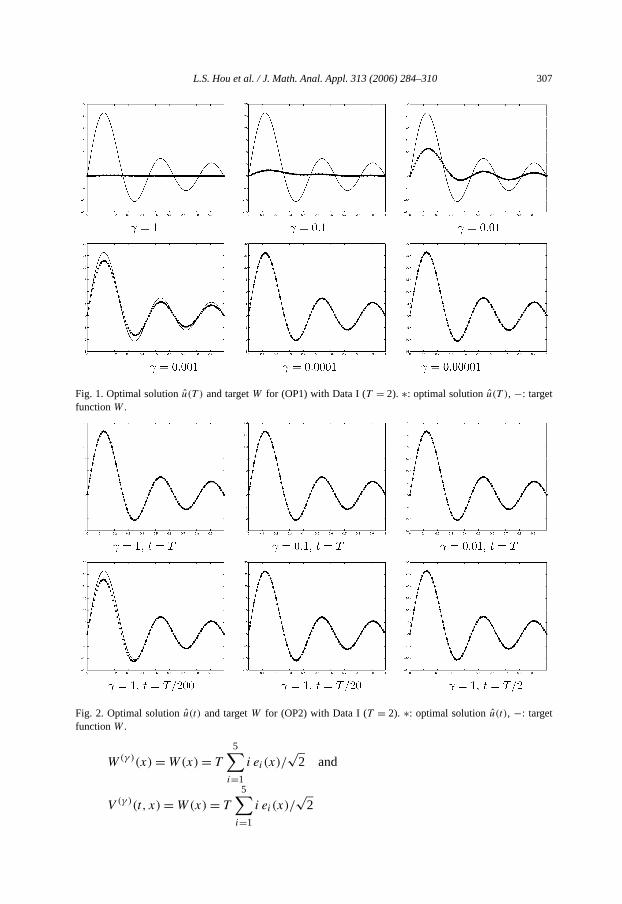
For each data set we solve (OP1) by series solution formulae (4.1)–(4.2). In eacwe vary the parameterγ and plot the optimal solutionu at the terminal timeT (the “∗”curve) versus the target functionW (the “−” curve). See Figs. 1 and 3.

For each data set we solve (OP2) by series solution formulae (4.9)–(4.10). In thof Data I, we choose


Fig. 1. Optimal solutionu(T ) and targetW for (OP1) with Data I (T = 2). ∗: optimal solutionu(T ), −: targetfunctionW .

Fig. 2. Optimal solutionu(t) and targetW for (OP2) with Data I (T = 2). ∗: optimal solutionu(t), −: targetfunctionW .

W(γ )(x) = W(x) = T

5∑i=1

i ei(x)/√

2 and

V (γ )(t, x) = W(x) = T

5∑i ei(x)/

√2

i=1


n the

d-

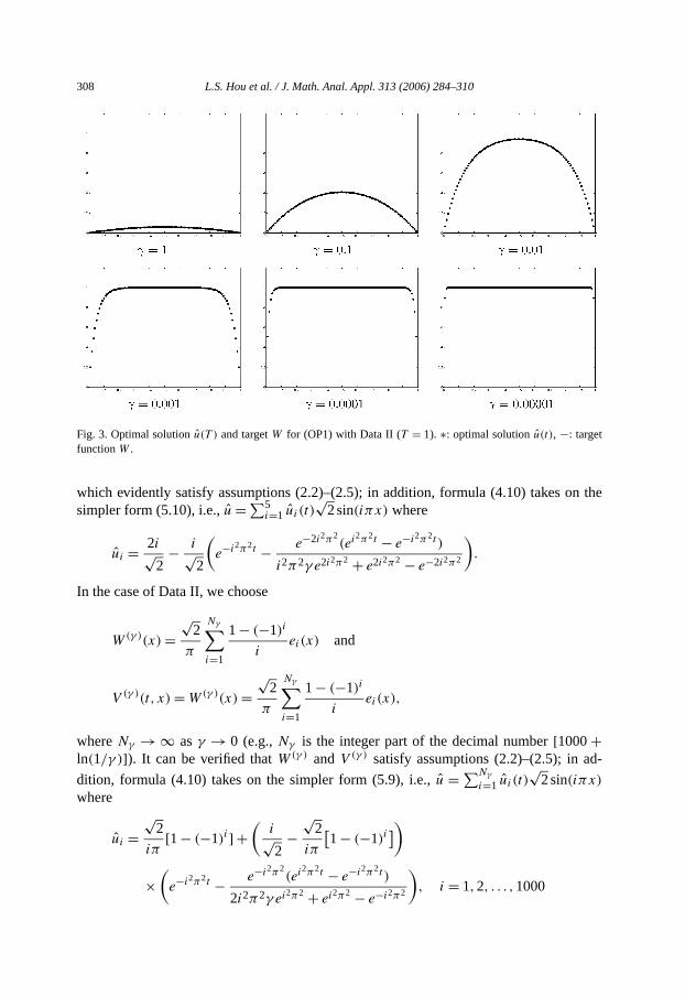
Fig. 3. Optimal solutionu(T ) and targetW for (OP1) with Data II (T = 1). ∗: optimal solutionu(t), −: targetfunctionW .

which evidently satisfy assumptions (2.2)–(2.5); in addition, formula (4.10) takes osimpler form (5.10), i.e.,u = ∑5

i=1 ui (t)√

2 sin(iπx) where

ui = 2i√2

− i√2

(e−i2π2t − e−2i2π2

(ei2π2t − e−i2π2t )

i2π2γ e2i2π2 + e2i2π2 − e−2i2π2

).

In the case of Data II, we choose

W(γ )(x) =√

2

π

Nγ∑i=1

1− (−1)i

iei(x) and

V (γ )(t, x) = W(γ )(x) =√

2

π

Nγ∑i=1

1− (−1)i

iei(x),

whereNγ → ∞ asγ → 0 (e.g.,Nγ is the integer part of the decimal number[1000+ln(1/γ )]). It can be verified thatW(γ ) andV (γ ) satisfy assumptions (2.2)–(2.5); in a

dition, formula (4.10) takes on the simpler form (5.9), i.e.,u = ∑Nγ

i=1 ui (t)√

2 sin(iπx)

where

ui =√

2

iπ[1− (−1)i] +

(i√2

−√

2

iπ

[1− (−1)i

])

×(

e−i2π2t − e−i2π2(ei2π2t − e−i2π2t )

2i2π2γ ei2π2 + ei2π2 − e−i2π2

), i = 1,2, . . . ,1000


l

case

ptimal

n

condi-state

ts andid a

atch-.4

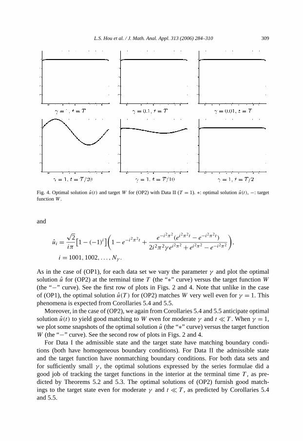
Fig. 4. Optimal solutionu(t) and targetW for (OP2) with Data II (T = 1). ∗: optimal solutionu(t), −: targetfunctionW .

and

ui =√

2

iπ

[1− (−1)i

](1− e−i2π2t + e−i2π2

(ei2π2t − e−i2π2t )

2i2π2γ ei2π2 + ei2π2 − e−i2π2

),

i = 1001,1002, . . . ,Nγ .

As in the case of (OP1), for each data set we vary the parameterγ and plot the optimasolution u for (OP2) at the terminal timeT (the “∗” curve) versus the target functionW(the “−” curve). See the first row of plots in Figs. 2 and 4. Note that unlike in theof (OP1), the optimal solutionu(T ) for (OP2) matchesW very well even forγ = 1. Thisphenomena is expected from Corollaries 5.4 and 5.5.

Moreover, in the case of (OP2), we again from Corollaries 5.4 and 5.5 anticipate osolutionu(t) to yield good matching toW even for moderateγ andt T . Whenγ = 1,we plot some snapshots of the optimal solutionu (the “∗” curve) versus the target functioW (the “−” curve). See the second row of plots in Figs. 2 and 4.

For Data I the admissible state and the target state have matching boundarytions (both have homogeneous boundary conditions). For Data II the admissibleand the target function have nonmatching boundary conditions. For both data sefor sufficiently smallγ , the optimal solutions expressed by the series formulae dgood job of tracking the target functions in the interior at the terminal timeT , as pre-dicted by Theorems 5.2 and 5.3. The optimal solutions of (OP2) furnish good mings to the target state even for moderateγ and t T , as predicted by Corollaries 5and 5.5.


–558.equa-

ear

904.

h. 19

nsion,

equa-

trol,

, Acta

, Acta

d dis-

vier–

erlin,

-Verlag,

v. 30

qua-

gress

ptimal

nction,

References

[1] L. Bal’chuk, Optimal control of systems described parabolic equations, SIAM. J. Control 7 (1969) 546[2] Y. Cao, M. Gunzburger, J. Turner, The controllability of systems governed by parabolic differential

tions, J. Math. Anal. Appl. 215 (1997) 174–189.[3] J.I. Diaz, A. Fursikov, A simple proof of the approximate controllability from the interior for nonlin

evolution problems, Appl. Math. Lett. 7 (1994) 85–87.[4] Y.V. Egorov, Some problems in the theory of optimal control, Soviet Math. 3 (1962) 1080–1084.[5] Y.V. Egorov, Some problems in the theory of optimal control, Zh. Vychisl. Mat. Mat. Fiz. 5 (1963) 887–[6] L. Evans, Partial Differential Equations, Amer. Math. Soc., Providence, RI, 1998.[7] H. Fattorini, Control in finite time of differential equations in Banach space, Comm. Pure Appl. Mat

(1966) 7–34.[8] H. Fattorini, D. Russell, Exact controllability theorems for linear parabolic equations in one space dime

Arch. Ration. Mech. Anal. 49 (1971) 272–292.[9] A. Fursikov, O. Imanuvilov, On exact boundary zero controllability of two-dimensional Navier–Stokes

tions, Acta Appl. Math. 36 (1994) 1–10.[10] A. Fursikov, O. Imanuvilov, On controllability of certain systems stimulating a fluid flow, in: Flow Con

in: IMA Vol. Math. Appl., vol. 68, Springer-Verlag, New York, 1995, pp. 149–184.[11] R. Glowinski, J.-L. Lions, Exact and approximate controllability for distributed parameter systems

Numer. (1994) 269–378.[12] R. Glowinski, J.-L. Lions, Exact and approximate controllability for distributed parameter systems

Numer. (1995) 159–333.[13] M. Gunzburger, S. Manservisi, The velocity tracking problem for Navier–Stokes flows with bounde

tributed controls, SIAM J. Control Optim. 37 (1999) 1913–1945.[14] M. Gunzburger, S. Manservisi, Analysis and approximation of the velocity tracking problem for Na

Stokes flows with distributed control, SIAM J. Numer. Anal. 37 (2000) 1481–1512.[15] J.-L. Lions, Optimal Control of Systems Governed by Partial Differential Equations, Springer-Verlag, B

1971.[16] J.-L. Lions, E. Magenes, Nonhomogeneous Boundary Value Problems and Applications, Springer

Berlin, 1972.[17] J.-L. Lions, Exact controllability, stabilization and perturbations for distributed systems, SIAM Re

(1988) 1–68.[18] D. Russell, A unified boundary controllability theory for hyperbolic and parabolic partial differential e

tions, Stud. Appl. Math. 52 (1973) 189–211.[19] D. Russell, Controllability and stabilizability theory for linear partial differential equations: Recent pro

and open questions, SIAM Rev. 20 (1978) 639–739.[20] D. Russell, Some remarks on numerical aspects of coefficient identification in elliptic systems, in: O

Control of Partial Differential Equations, Birkhäuser, Boston, MA, 1984, pp. 210–228.[21] R. Temam, Navier–Stokes Equations, Amer. Math. Soc./Chelsea, Providence, RI, 2001.[22] T. Tsachev, Optimal control of linear parabolic equation: The constrained right-hand side as control fu

Numer. Funct. Anal. Optim. 13 (1992) 369–380.

eigen series solutions to terminal-state tracking optimal control problems and exact controllability...

Documents