EHA: Terminology and basic non-parametric graphs

Sociology 229 Advanced Regression

Class 4

Copyright © 2010 by Evan Schofer

Do not copy or distribute without permission

Announcements

• Assignment 2 Due• Assignment 3 handed out

• Agenda:• Event history analysis – basic issues.

Review: Why we need EHA

• Example: Drug dosage and mortality

• Question: What are the limits of using OLS regression to model time-to-mortality?– Answer:

• Censoring: some patients don’t die• Violation of normality assumptions: outcome variable

is not normal– This also causes issues for “censored normal regression”

– Question: What about Logistic Regression?• Answer: Fails to utilize information on timing.

Motivation

• Event history analysis is more than just a “fix” for censoring and violations of normality…– EHA concepts and data structures put “dynamic”

processes at the foreground• In short, EHA helps us think about how time matters.

EHA: Overview and Terminology

• EHA is referred to as “dynamic” modeling• i.e., addresses the timing of outcomes: rates

• Dependent variable is best conceptualized as a rate of some occurrence

• Not a “level” or “amount” as in OLS regression• Think: “How fast?” “How often?”

• The “occurrence” may be something that can occur only once for each case: e.g., mortality

• Or, it may be repeatable: e.g., marriages, strategic alliances.

EHA: Types of Questions

• Some types of questions EHA can address:

• 1. Mortality: Does drug dosage reduce rates?• Does “rate” decrease with larger doses?• Also: control for race, gender, treatment options, etc

• 2. Life stage transitions: timing of marriage• Is rate affected by gender, class, religion?

• 3. Organizational mortality• Is rate affected by size, historical era, competition?

• 4. Inter-state war• Is rate affected by economic, political factors?

EHA: Overview

• EHA involves both descriptive and parametric analysis of data

• Just like regression:• Scatterplots, partialplots = descriptive• OLS model/hypothesis tests = parametric

– Descriptive analyses/plots• Allow description of the overall rate of some outcome• For all cases, or for various subgroups

– Parametric Models • Allow hypothesis testing about variables that affect

rate (and can include control variables).

EHA Terminology: States & Events

• EHA has evolved its own terminology:

• “State” = the “state of being” of a case• Conceptualized in terms of discrete phenomena• e.g., alive vs. dead

• “State space” = the set of all possible states• Can be complex: Single, married, divorced, widowed

• “Event” = Occurrence of the outcome• Also called “transition”, “failure”• Shift from “alive” to “dead”, “single” to “married”• Occurs at a specific, known point in time

Terminology: Risk & Spells

• “Risk Set” = the set of all cases capable of experiencing the event

• e.g., those “at risk” of experiencing mortality• Note: the risk often changes over time

– Shrinks as cases experience events– Or grows, if new cases enter the study

• “Spell” = A chunk of time that a case experiences, bounded by: events, and/or the start or end of the study

• As in “I’m gonna sit here for a spell…”• Sometimes called a “duration”.

States, Spells, & Events: Visually

• If we assign numeric values to states, it is easy to graph cases over time

• As they experience 1 or more spells

• Example: drug & mortality study

• States:• Alive = 0• Dead = 1

• Time = measured in months• Starting at zero, when the study begins• Ending at 60 months, when study ends (5 years).

States, Spells, & Events: Visually

• Example of mortality at month 33

1

0

0 10 20 30 40 50 60 Time (Months)

Sta

te Spell #1

Spell #2

EventEnd of Study

• Note: It takes 2 spells to describe this case– But, we may only be interested in the first spell. (Because there is no

possibility of change after transition to state = 1)

States, Spells, & Events: Visually

• Example of a patient who is cured– Doesn’t experience mortality during study

1

0

0 10 20 30 40 50 60 Time (Months)

Sta

te Spell #1

End of Study

• Note: Only 1 spell is needed– The spell indicates a consistent state (0), for the

period of time in which we have information

More Terminology: Censoring

• Note: In both cases, data runs out after month 60

• Even if the patient is still alive

• In temporal analysis, we rarely have data for all relevant time for all cases

• “Censored” = indicates the absence of data before or after a certain point in time

• As in: “data on cases is censored at 60 months”

• “Right Censored” = no data after a time point

• “Left Censored” = no data before a time point

States, Spells, & Events: Visually

• A more complex state space: marital status• 0 = single, 1 = married, 2 = divorced, 3 = widowed

• Individual history:• Married at 20, divorced at 27, remarried at 33

3

2

1

0

16 20 24 28 32 36 40 44Age (Years)

Sta

te

Spell #1Right

Censored at 45

Spell #4Spell #2 Spell #3

Measuring States and Times

• EHA, in short, is the analysis of spells• It takes into account the duration of spells, and

whether or not there was a change of state at the end

• States at start and end of spell are measured by assigning pre-defined values to a variable

• Much like logit/probit or multinomial logit

• Times at the start and end of spell must also be measured

• Time Unit = The time metric in the study• e.g., minutes, hours, days, months, years, etc

Time Clock

• Time Clock = time reference of the analysis

• Possibilities:• Duration since start of study• Chronological age of case (person, firm, country)• Duration since end of last spell

– i.e., clock is set to zero at start of each spell

• Historical time – the actual calendar date

• The choice of time-clock can radically change the analysis and meaning of results

• It is crucial to choose a clock that makes sense for the hypotheses you wish to test

Time Clocks Visually: Age

3

2

1

0

16 20 24 28 32 36 40 44Age (Years)

Sta

te

Spell #1End of StudySpell #4Spell #2 Spell #3

• EHA examines rate of transitions as a function of a person’s age

Time Clocks Visually: Duration Single from 16-20 (4 years), married from 20-27 (7 years),

divorced from 27-33 (6 yrs), remarried at 33-45 (12 yrs)

3

2

1

0

0 4 6 12 18 22 Duration (Years)

Sta

te

Spell #1

Spell #4Spell #2 Spell #3

• EHA examines rate of transitions as a function of a person’s duration in their current state

Time Clocks: General Advice

• Different time-clocks have different strengths• We’ll discuss this more…

• Chronological Age = good for processes clearly linked to age

• Biological things: fertility, mortality• Liability of newness

• Historical time = useful for examining the impact of historical change on ongoing phenomena

• E.g., effects of changing regulatory regimes on rates of strategic alliances

Moving Toward Analyses: Example

• Example: Employee retention• How long after hiring before employees quit?

• Data: Sample of 12 employees at McDonalds

• Time-Clock/Time Unit: duration of employment from time of hiring (measured in days)

• 2 Possible states:• Employed & No longer employed

• We are uninterested in subsequent hires• Therefore, we focus on initial spell, ending in quitting.

Example: Employee Retention

• Visually – red line indicates length of employment spell for each case:

0 20 40 60 80 100 120 Time (days)

Cas

es

Right Censored

Simple EHA Descriptives

• Question: What simple things can we do to describe this sample of 12 employees?

• 1. Average duration of employment• Only works if all (or nearly all) have quit• Many censored cases make “average” meaningless

– This is a fairly useful summary statistic• Gives a sense of overall speed of events• Especially useful when broken down by sub-groups• e.g., average by gender or compensation plan.

Descriptives: Average Duration

• Simply calculate the mean time-to-quitting

0 20 40 60 80 100 120 Time (days)

Cas

es

Right Censored

Average = 33.4 days

Simple EHA Descriptives

• Question: What simple things can we do to describe this sample of 12 employees?

• 2. Compute “Half Life” of employee tenure– i.e., median failure time… a better option than “mean”

• Determine time at which attrition equals 50%• Also highlights the overall turnover rate• Note: Exact value is calculable, even if there are

censored cases• Again, computing for sub-groups is useful

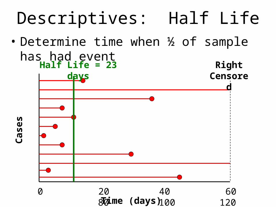
Descriptives: Half Life• Determine time when ½ of sample has had

event

0 20 40 60 80 100 120 Time (days)

Cas

es

Right Censored

Half Life = 23 days

Simple EHA Descriptives

• Question: What simple things can we do to describe this sample of 12 employees?

• 3. Tabulate (or plot) quitters in different time-periods: e.g., 1-20 days, 21-40 days, etc.

• Absolute numbers of “quitters” or “stayers”– or

• Numbers of quitters as a proportion of “stayers”• Or look at number (or proportion) who have “survived”

(i.e., not quit)

Descriptives: Tables• For each period, determine number or

proportion quitting/staying

0 20 40 60 80 100 120 Time (days)

Cas

es

Day 1-20 20-40 40-60 60-80 80-100

EHA Descriptives: TablesTime Range

Quitters:

Total #, %

# staying

1 Day 1-20 5 quit, 42% of all,

42% of remaining

7 left, 58 % of all

2 Day 21-40 2 quit, 16% of all

29% of remaining

5 left, 42% of all

3 Day 41-60 1 quit, 8% of all

20% of remaining

4 left, 33 % of all

4 Day 61-80 1 quit, 8% of all

25% of remaining

3 left, 25% of all

EHA Descriptives: Tables

• Remarks on EHA tables:

• 1. Results of tables change depending on time-ranges chosen (like a histogram)

• E.g., comparing 20-day ranges vs. 10-day ranges

• 2. % quitters vs. % quitters as a proportion of those still employed

• Absolute % can be misleading since the number of people left in the risk set tends to decrease

• A low # of quitters can actually correspond to a very high rate of quitting for those remaining in the firm

• Typically, these ratios are more socially meaningful than raw percentages.

EHA Descriptives: Plots

• We can also plot tabular information:

0

10

20

30

40

50

60

70

80

90

100

0 1 2 3 4 5

Time Period

Pe

rce

nt

% Quit (of Remaining)

% Remaining

The Survivor Function: S(t)

• A more sophisticated version of % remaining• Calculated based on continuous time (calculus), rather

than based on some arbitrary interval (e.g., day 1-20)

• Survivor Function – S(t): The probability (at time = t) of not having the event prior to time t.

• Always equal to 1 at time = 0 (when no events can have happened yet

• Decreases as more cases experience the event• When graphed, it is typically a decreasing curve• Looks a lot like % remaining

Survivor Function: S(t)

• McDonald’s Example:Survivor Function: McDonalds Employees

0

0.1

0.2

0.3

0.4

0.5

0.6

0.7

0.8

0.9

1

0 20 40 60 80 100 120

Time

S(t

)

Steep decreases indicate lots of

quitting at around 20 days

Survivor Function: S(t)

• Interpretation: The survivor function reflects the probability of surviving beyond time t

• A monotone, non-increasing function of time• Always starts at 1, decreases as cases experience

events

• Let’s try to draw some possible survivor functions

• For human mortality• For the failure of a computer hard-drive• For having a (first) baby• For large US cities having major protests in the civil

rights movement.

Survivor Ex: First Marriage

• Compare survivor for women, men:Kaplan-Meier survival estimates, by dfem

analysis time0 50 100

0.00

0.25

0.50

0.75

1.00

dfem 0

dfem 1

Survivor plot for Men

(declines later)

Survivor plot for Women

(declines earlier)

The Hazard Function: h(t)

• A more sophisticated version of # events divided by # remaining

• Hazard Function – h(t) = The probability of an event occurring at a given point in time, given that it hasn’t already occurred

• Formula:

t

tTtTttPth

t

)(lim)(

0

• Think of it as: the rate of events occurring for those at risk of experiencing the event

The Hazard Function

• Example:McDonalds Employees: Hazard Rate

0.00

0.02

0.04

0.06

0.08

0.10

0.12

0.00 10.00 20.00 30.00 40.00 50.00 60.00 70.00 80.00

Time

h(t

)

High (and wide) peaks indicate lots of quitting

The Hazard Function: h(t)

• Interpretation: The hazard function reflects the rate of events at a given point in time

• For cases that made it that far…• It reflects the “rate that risk is accumulating”

• Let’s draw some hazard functions• For human mortality• For the failure of a computer hard-drive• For having a (first) baby• For large US cities having major protests in the civil

rights movement.

Figure 3. Estimated hazard rateof entry into first marriage for entire sample

Est

ima

ted

Ha

zard

Ra

te

Age in Years12 20 30 40 50 60 70 80

12 20 30 40 50 60 70 80

0

.05

.1

.15

.2

0

.05

.1

.15

.2

Hazard Plot: First Marriage• Hazard Rate: Full Sample

Cumulative Hazard Function: H(t)

• The “cumulative” or “integrated” hazard• Use calculus to “integrate” the hazard function• Recall – An integral represents the area under the

curve of another function between 0 and t

– Hazard is a rate, like “60 miles per hour”• Integrated hazard is total distance driven…• In three hours, it would be 180 miles

– Integrated hazard functions always increase (opposite of the survivor function).

• Big increases indicates that the hazard is high

Cumulative Hazard Function: H(t)

• Example:McDonalds Employees: Integrated Hazard

0

0.2

0.4

0.6

0.8

1

1.2

1.4

1.6

1.8

0 20 40 60 80 100

Time

Inte

gra

ted

Haz

ard

Steep increases indicate peaks in

hazard rate

“Flat” areas indicate low hazard rate

The Cumulative Hazard: H(t)

• Interpretation: The cumulative hazard function reflects the total amount of risk that has accumulated at a given point in time…

• Let’s draw some integrated hazard functions• For human mortality• For the failure of a computer hard-drive• For having a (first) baby• For large US cities having major protests in the civil

rights movement.

Integrated Hazard: First Marriage

• Compare Integrated Hazard for women, men:Nelson-Aalen cumulative hazard estimates, by dfem

analysis time0 50 100

0.00

1.00

2.00

3.00

dfem 0

dfem 1

Integrated Hazard for men increases slower (and remains lower)

than women

Cumulative Hazard Example• Ex: Edelman et al. 1999: EEOC Grievance procedures

EHA Plots: Remarks

• Plotting EHA data is extremely useful• Helps you understand your data• Helps you figure out the correct time-clock• Helps you to develop arguments about dynamics• Allows you to compare different groups

– We’ll pick this up in the future.