processes

Article

Efficient Two-Step Parametrization of a Control-OrientedZero-Dimensional Polymer Electrolyte Membrane Fuel CellModel Based on Measured Stack Data

Zhang Peng Du 1,* , Christoph Steindl 2 and Stefan Jakubek 1

Citation: Du, Z.P.; Steindl, C.;

Jakubek, S. Efficient Two-Step

Parametrization of a Control-

Oriented Zero-Dimensional Polymer

Electrolyte Membrane Fuel Cell

Model Based on Measured Stack Data.

Processes 2021, 9, 713. https://

doi.org/10.3390/pr9040713

Academic Editor: Alessandro

D’ Adamo

Received: 23 March 2021

Accepted: 15 April 2021

Published: 18 April 2021

Publisher’s Note: MDPI stays neutral

with regard to jurisdictional claims in

published maps and institutional affil-

iations.

Copyright: © 2021 by the authors.

Licensee MDPI, Basel, Switzerland.

This article is an open access article

distributed under the terms and

conditions of the Creative Commons

Attribution (CC BY) license (https://

creativecommons.org/licenses/by/

4.0/).

1 Institute of Mechanics and Mechatronics, Technische Universität Wien, Getreidemarkt 9,1060 Vienna, Austria; stefan.jakubek@tuwien.ac.at

2 Institute of Powertrains and Automotive Technology, Technische Universität Wien, Getreidemarkt 9,1060 Vienna, Austria; christoph.steindl@tuwien.ac.at

* Correspondence: zhang.peng.du@tuwien.ac.at; Tel.: +43-1-58801-325540

Abstract: This paper proposes a new efficient two-step method for parametrizing control-orientedzero-dimensional physical polymer electrolyte membrane fuel cell (PEMFC) models with measuredstack data. Parametrizations of these models are computationally intensive due to the numerous un-known parameters and the typically nonlinear, stiff model properties. This work reduces an existingmodel to decrease its stiffness for accelerated numerical simulations. Subdividing the parametrizationinto two consecutive subproblems (thermodynamic and electrochemical ones) reduces the solutionspace significantly. A parameter sensitivity analysis further reduces each sub-solution space by ex-cluding non-significant parameters. The method results in an efficient parametrization process. Thetwo-step approach minimizes each sub-solution space’s dimension by two-thirds, respectively three-fourths, compared to the global one. An achieved R2 value between simulation and measurement of91% on average provides the required accuracy for control-oriented models.

Keywords: polymer electrolyte membrane fuel cell; control-oriented model; grey-box modeling;analytical differentiability; model reduction; parameter sensitivity analysis; fisher information;efficient parameterization; data-driven identification; transient operation measurement data

1. Introduction

PEMFCs are promising candidates for replacing internal combustion engines in mobileapplications. However, fuel cell (FC) driven vehicles are still far from having a significantmarket share because of various challenges. One of the challenges is to control the FCduring transient operations, especially regarding avoiding harmful operating conditions.Another one is to improve the FC system’s efficiency via optimal control. Moreover, experi-mental expenditures during development are high but are reducible by using simulationsinstead. One of the first steps towards resolving the named and other challenges is obtain-ing a proper FC model. PEMFCs are promising candidates because they offer the rapidstartup and low operating temperature required for automotive applications. However, itrequires appropriate water management to address liquid water formation. Solid oxideFCs use non-noble metal catalysts, which results in low raw material costs, but the highoperating temperature leads to thermal stress and precludes this FC for transient applica-tions. Molten carbonate FCs can reform a wide variety of fuel sources, but the long startuptime eliminates this FC for anything but continuous-power applications. Phosphoric acidFCs provide easy water management, but the low power density is not appropriate forportable applications. Alkaline FCs have the highest demonstrated operating efficiencyof any FC system, but the intolerance to carbon dioxide forces the use of carbon dioxideremoval equipment and pure oxygen and hydrogen [1].

In general, modeling approaches are distinguishable into three groups. First, black-boxmodeling means fitting an artificial model to replicate the measured input and output data

Processes 2021, 9, 713. https://doi.org/10.3390/pr9040713 https://www.mdpi.com/journal/processes

Processes 2021, 9, 713 2 of 18

correlation [2–4]. The model structure and parameters do not need to have any physicalmeaning, and extrapolation capabilities are limited. Black-box models, in general, do notreplicate internal unmeasured physical states. Second, white-box models solely describe theFC with first principles known from theory. All model parameters are physical quantities,fundamental constants, and known values. Measurement data is not needed [5–7]. Thisapproach is not feasible if not every parameter is known, which is usually the case for FCmodels. Third, grey-box models combine both approaches. They use the first principlesknown from theory and require measurement data to determine the model structure andparameters. This work does not consider black-box models because the internal states’knowledge is essential for the controller to avoid harmful operating conditions. White-boxmodels are unsuitable because many parameters are unknown. Therefore the combinationof both approaches, grey-box models, provides the needed structure and fidelity for FCcontrol. Control-oriented grey-box PEMFC models aim to have a low spatial dimension tobe numerically efficient for real-time applications [8–12]. Parametrizing grey-box PEMFCmodels is not straightforward because they are nonlinear, numerically stiff, and havenumerous unknown parameters. This work proposes an efficient two-step parametrizationmethod that drastically simplifies the optimization problem. The method subdivides theFC model into two submodels for parametrization, each yielding a lower-dimensionalsub-solution space compared to the one of the entire model.

The standard parametrization procedure determines as many parameters as possiblefrom theory, datasheets, and expert knowledge. The remaining unknown parameters haveto be obtainable by fitting measurement data. For example, McKay et al. [13] developed alumped parameter model, and they identified the tunable parameters using least squares.Unfortunately, this approach yields a high dimensional solution space for models withmany unknown parameters. The proposed multiple-step method by Xu et al. [14] estimatesthe nozzle coefficients first, and in the following step, a nonlinear least-squares algorithmidentifies the electrochemical parameters for a steady-state voltage response. Additionally,a fitted neural network describes the dependency of the electrochemical parameters on theoperating conditions. Using a neural network is suboptimal because the applicability ishighly limited to the range of the available measurement data. Müller et al. [15] conductedan approximated sensitivity analysis by varying the signals and parameters. The sensitivityanalysis’s sole purpose was to show the importance of accurate sensors for parametrization.They used specific measurements to identify parameters one by one. Curve fitting leads tothe remaining parameters. Individually estimating the parameters is not always feasiblebecause it is strongly dependent on the available measurement data and model structure.Moreover, incorporating the sensitivity analysis into the parametrization process will in-crease its efficiency, especially for large-scale problems. Goshtasbi et al. [16] approximatedthe parameter sensitivities via difference quotients. In [17], the sensitivity analysis deter-mines the most sensitive parameters for identification, and a global optimizer identifies thissubset of parameters altogether. This approach’s drawback is that a large subset still leadsto a computationally-intensive problem. In [18], the authors used the parameter sensitivityanalysis to divide the parameters into three groups. The groups contain the identifiableparameters in the low, medium, and high current regions, respectively. Unfortunately,this approach needs appropriately designed experiments. Ritzberger et al. [9] developeda PEMFC model focusing on its analytical differentiability. Existing models are usuallynot analytical differentiable but are transformable to a model with this property. Analyticdifferentiability enables an accurate and efficient calculation of the derivatives comparedto a numerical approximation and is advantageous for various control applications. Theylocally linearized the nonlinear model in multiple operating points. Their proposed pa-rameterization method optimizes each analytically linearized model for each operatingpoint dependent on the same parameter set simultaneously. In [10], they additionallyconducted a parameter sensitivity analysis based on the analytically linearized models.This approach’s disadvantage is that it is limited to data with small excitations because of

Processes 2021, 9, 713 3 of 18

the linearization. Therefore it requires specially designed experiments, which is mostly notthe case for given data.

In this work, the two-step parameterization method is demonstrated with the modeldeveloped by Ritzberger et al. [10] because of its advantageous property of analyticaldifferentiability. The model is adapted to reduce its stiffness for more efficient numeri-cal evaluations. Subdividing the model into a thermodynamic and an electrochemicalsubmodel leads to a parameterization method with two consecutive steps. In the firststep, the thermodynamic submodel, which consists of a system of first-order ordinarydifferential equations (ODEs), is parametrized. The electrochemical submodel, which doesnot have any ODEs, is parametrized in the following second step. The subdivision reducesthe solution space’s dimension for each submodel, and an analytic parameter sensitivityanalysis further reduces each parameter subset by excluding non-significant parameters. Aglobal optimizer identifies the parameter subsets by minimizing the difference betweensimulated and measured output signals [19]. An existing FC test bench delivers the mea-surement data. Compared to the available approaches, this efficient method simplifies theparametrization problem, it does not require appropriately designed experiments, and theparameter sensitivity analysis is analytically evaluable.

This paper is subsequently structured as follows: Section 2 describes the PEMFCmodel and its reduction. Section 3 presents the two-step parametrization method, explainsthe parameter sensitivity analysis, and shows the proposed method’s validation. Section 4depicts the experimental setup, and finally, Section 5 discusses the identification results.

2. Fuel Cell Model

This section briefly portrays the used PEMFC model to demonstrate the proposedtwo-step parametrization method. Additionally, this section describes the model reductionfor accelerated numerical simulations. The proposed method is, of course, not limited tothe described FC model. Any model separable into a submodel with ODEs and a submodelwithout ODEs is utilizable. The model does not have to be analytically differentiable be-cause the parameter sensitivity analysis is numerically approximable. However, numericalapproximations are less efficient and accurate evaluable than analytical solutions.

2.1. Model Description

Ritzberger et al. [10] developed the model, and it is an adapted version of the Pukrush-pan et al. [8] model. The difference is that the adapted model has the property of analyticaldifferentiability, which is the reason for its selection. This property is beneficial for variouscontrol methodologies [20,21], and parameter sensitivity analyses (Section 3.2). The modelis a zero-dimensional physical PEMFC model, and Figure 1 gives a schematic overview.It utilizes, amongst others, mass balances, linear nozzle equations, diffusion equations,electrochemical equations, and the ideal gas law [22–24]. However, it does not considerenergy balances and thus cannot model the FC temperature over time. The model treatsthe measured temperature as an input. This temperature is assumed to be the uniformtemperature for the whole FC. The model consists of a cathode, anode, membrane, andelectrochemical submodel, which are interconnected. The model equations and theirderivations are not the focus of this work. More information in this regard is availablein [10].

The cathode submodel has four mass states (oxygen mass mca,O2 , nitrogen mass mca,N2 ,vapor mass mca,vap, and liquid water mass mca,liq) and two pressure states (supply manifoldpressure pca,sm, and exit manifold pressure pca,em). The anode submodel also has four massstates (hydrogen mass man,H2 , nitrogen mass man,N2 , vapor mass man,vap, and liquid watermass man,liq) but only one pressure state (exit manifold pressure pan,em). The membranesubmodel only has the membrane water activity state am. The model inputs are the airmass flow mca,in, the hydrogen mass flow man,in, the anode supply manifold pressurepan,sm, the relative humidity of the air mass flow ϕca,in, the purging signal αpurge, the FCtemperature T, the atmospheric pressure patm, and the current I. The outputs are the

Processes 2021, 9, 713 4 of 18

cathode supply manifold pressure pca,sm, the cathode exit manifold pressure pca,em, theanode exit manifold pressure pan,em, and the voltage U. Hence, the following equationsdescribe the nonlinear FC state-space model:

xnr = fnr(xnr, u, θ) (1)

y = gnr(xnr, u, θ) (2)

Figure 1. Schematic overview of the model structure of the lumped, transient FC stack model [10].

Here, xnr = xnr(t) denotes the non-reduced state vector, u = u(t) the input vector,y = y(t) the output vector, θ ∈ R25 the parameter vector, fnr the non-reduced systemfunction, gnr the non-reduced output function, and t the time [25]. The respective vectorsare structured as follows:

xnr =

pca,smmca,O2mca,N2

mca,vapmca,liqpca,emman,H2

man,N2

man,vapman,liqpan,em

am

, u =

mca,inman,inpan,smϕca,inαpurge

Tpatm

I

, y =

pca,smpca,empan,em

U

, θ =

[Vca,sm, Vca,cm, Vca,em, . . .. . . Van,sm, Van,cm, Van,em, . . .. . . kperm, kcond, kevap, . . .. . . kca,sm,out, kca,em,in, . . .. . . kca,em,out, kan,sm,out, . . .. . . kan,em,in, kan,em,out, . . .. . . kan,leak, τm, . . .. . . ε2, Rc, Eca,act, Ean,act, . . .. . . Kca, Kan, CDca, CDan]T

(3)

V denotes the volumes, k the nozzle or mass flow coefficients, τm the water activity timeconstant, ε2 the membrane conductivity parameter, Rc the ohmic contact resistance, E

Processes 2021, 9, 713 5 of 18

the energy, K the intrinsic exchange current parameter, and CD the combined diffusioncoefficient. Compared to the model described by Ritzberger et al. [10], this one has anadditional output, the cathode exit manifold pressure pca,em. It is measured, thereforeconsidering it as a supplementary output has the advantage that it yields additional insightinto the system. Furthermore, the pressure difference between the exit manifold and theenvironment is too big to be sufficiently described by a linear nozzle equation. Hencenonlinear nozzle equations (derived from the Bernoulli equation) replace the linear ones ateach exit manifold.

2.2. Model Reduction

The model reduction goal in this work is to reduce the model’s stiffness for acceleratednumerical simulations. Lambert [26] stated that stiffness occurs when (numerical) stabilityrequirements, rather than those of accuracy, constrain the (simulation time) step length.The pressure dynamics of the model are faster by multiple orders of magnitude comparedto the mass dynamics. Thus the pressure dynamics are assumed to be steady-state at alltimes. The ODE for the cathode supply manifold pressure pca,sm results from a combinationof the ideal gas law and the mass balance

pca,sm =Rca,smTVca,sm

(mca,in − mca,sm,cm), (4)

where Rca,sm denotes the cathode supply manifold’s mass-specific gas constant, mca,sm,cm =kca,sm,out(pca,sm − pca,cm) the mass flow between the cathode supply and center manifold,kca,sm,out the cathode supply manifold’s outflow nozzle coefficient, and pca,cm the cathodecenter manifold pressure. Assuming steady-state, the ODE (4) transforms into

pca,sm =mca,in

kca,sm,out+ pca,cm. (5)

The exit manifold pressures of the cathode pca,em and anode pan,em are addressed in asimilar fashion leading to the reduced nonlinear FC state-space model given by

x = f(x, u, θ), (6)

y = g(x, u, θ). (7)

Here, f denotes the reduced system function, g the reduced output function, andx = x(t) the reduced state vector. The reduced state vector is structured as

x = [mca,O2 , mca,N2 , mca,vap, mca,liq, man,H2 , man,N2 , man,vap, man,liq, am]T, (8)

and it does not contain the three pressure states (pca,sm, pca,em, and pan,em) anymore.Theinput vector u, the output vector y, and the parameter vector θ remain unchanged. Thelongest integration step length of the reduced model, which still yields a stable solution,is about 50% longer than for the non-reduced model, leading to a roughly 36% shortersimulation time [27].

Processes 2021, 9, 713 6 of 18

3. Two-Step Parametrization Method3.1. Key Idea

The two-step parametrization method’s key idea is to subdivide the given nestedstate-space model (6) and (7) into two submodels. The nested model is separable in thefollowing way:

x = xth, f(x, u, θ) = fth(x, u, θth) (9)

y =

[yth

yel

]=

pca,smpca,empan,em

U

, g(x, u, θ) =

[gth(x, u, θth)

gel(x, u, θ)

](10)

The model’s parameter vector is divisible as well:

θ =

[θth

θel

]=

[Vca,sm, Vca,cm, Vca,em, . . .. . . Van,sm, Van,cm, Van,em, . . .

. . . kperm, kcond, kevap, . . .. . . kca,sm,out, kca,em,in, kca,em,out, . . .. . . kan,sm,out, kan,em,in, kan,em,out, . . .

. . . kan,leak, τm]T

[ε2, Rc, Eca,act, Ean,act, . . .. . . Kca, Kan, CDca, CDan]T

(11)

On the one hand, the subdivision yields the thermodynamic submodel

x = f(x, u, θth), (12)

yth = gth(x, u, θth), (13)

and on the other hand, it results in the electrochemical submodel

yel = gel(x, u, θ). (14)

The thermodynamic submodel (12) and (13) is only dependent on the thermodynamicparameter vector θth, which also holds for the system function f according to Equation (9).Therefore the electrochemical parameter vector θel does not affect the states x and thethermodynamic outputs yth, but only the electrochemical output yel. Thus the electro-chemical submodel (14) utilizes the full parameter vector θ = [θth, θel]

T. Note that thethermodynamic submodel consists of ODEs, and the electrochemical one does not. Thetwo-step parametrization method exploits the described properties.

3.2. Parameter Sensitivity Analysis

The FC model used in this work has numerous unknown parameters, which raisesthe question of whether each parameter is unambiguously identifiable. The parameteridentifiability is, in general, strongly dependent on the model structure and the availablemeasurement data. A parameter sensitivity analysis can aid in answering these questions,and the Fisher information matrix (FIM) F is well-established for conducting such analy-sis [28]. Under the assumption of Gaussian prediction errors with zero mean values andtime-independent covariances, the Cramér-Rao inequality holds [29]:

Cov(θ) F−1 (15)

The inequality says that the inverse of F is the lower bound of the parameter covari-ances. The first step for obtaining the FIM is computing the state parameter sensitivities

Processes 2021, 9, 713 7 of 18

ξi = dx/dθi, where θi for i ∈ 1, 2, . . . , nθ denotes a parameter, and nθ the number ofparameters. They are obtainable from solving the following first-order ODE:

ξi =ddt

(dxdθi

)=

ddθi

(dxdt

)=

ddθi

f(x, u, θ)

=∂f(x, u, θ)

∂xdxdθi

+∂f(x, u, θ)

∂θi

=∂f(x, u, θ)

∂xξi +

∂f(x, u, θ)

∂θi

(16)

The second step is to calculate the output parameter sensitivities ψi = dy/dθi with

ψi =∂g(x, u, θ)

∂xdxdθi

+∂g(x, u, θ)

∂θi

=∂g(x, u, θ)

∂xξi +

∂g(x, u, θ)

∂θi.

(17)

The model described by Ritzberger et al. [10] has analytic derivatives available, andthis work utilizes MATLAB R2020b’s Symbolic Math Toolbox [30] to compute them. Alloutput parameter sensitivities ψi merged into one matrix yields the output parametersensitivity matrix ψ(t) = [ψ1(t), ψ2(t), . . . , ψnθ

(t)]. The FIM is determinable with ψ(t)taken at the sample times tk for k ∈ 0, 1, . . . , nk, where nk + 1 is the number of sample in-stants. Finally, using the sampled output parameter sensitivity matrix ψ(tk), the FIM iscomputable with

F =nk

∑k=0

ψT(tk)Σ−1e ψ(tk), (18)

where Σe denotes the prediction error covariance matrix, and F ∈ Rnθ×nθ holds. Underthe assumption of a perfect model, the prediction error covariance Σe is identical to themeasurement noise covariance and thus assumed to be known.

According to the Crámer-Rao inequality (15), the inverse of the FIM is the lowerbound of the absolute parameter variances. Thus directly analyzing F would mean thatthe parameter‘s physical units and their magnitudes bias the analysis. Using the nor-malized dimensionless FIM Fnorm for a physical unit independent analysis resolves thisissue [31–33]:

Fnorm =

θ1 0 · · · 0

0 θ2. . .

......

. . . . . . 00 · · · 0 θnθ

F

θ1 0 · · · 0

0 θ2. . .

......

. . . . . . 00 · · · 0 θnθ

(19)

The identifiability of the parameters is theoretically derivable from the inverse ofFnorm. Unfortunately, this is not always feasible because the FIM is often ill-conditioned oreven singular. Using a singular value decomposition (SVD) of Fnorm resolves this issue andenables further analysis [32–34]:

Fnorm = UΣVT (20)

U denotes the matrix containing the left singular vectors, Σ = diag(σ1, σ2, . . . , σnθ) the

singular value matrix, and V the matrix containing the right singular vectors. The leftand the right singular vector matrix are identical because Fnorm is a symmetric matrix.The analysis utilizes the right singular vector matrix V = [v1, v2, . . . , vnθ

], where vl forl ∈ 1, 2, . . . , nθ denotes a singular vector corresponding to the singular value σl . Thesingular values are interpretable as the amount of information, and the correspondingsingular vectors determine the direction in the parameter space. The Euclidean norm of thevectors is 1. Thus the relative direction share of the vector component vl,i is v2

l,i [35]. Therelative direction v2

l,i multiplied with the singular value σl is the amount of information

Processes 2021, 9, 713 8 of 18

showing into the parameter θi’s direction. Summing up all the information of one parameterfrom each singular value yields the parameter’s total information

σθi =nθ

∑l=1

v2l,iσl . (21)

The parameter’s total information σθi indicates if a parameter is identifiable with thegiven model and measurement data. The most significant parameters θms are determinableby sorting the parameters according to their total information in descending order. Themost significant parameters are determined by summing up the first nθms parameters untilthe following inequality holds:

∑nθmsi=1 σθms,i

∑nθi=1 σθi

≥ γ (22)

Note that γ ∈ [0, 1] denotes the threshold and is adaptable for different purposes.This work uses γ = 0.99999. In this case, the most significant parameters θms describe≥99.999% of Fnorm, and the least significant ones θls describe ≤0.001%, which makes thelatter negligible for parametrization.

3.3. Procedure

The proposed method parametrizes the model in two consecutive main steps:

1. Thermodynamic submodel

(a) Parameter sensitivity analysis with respect to the thermodynamic parame-ters θth yields a subset with the most significant parameters θth,ms, whereθth,ms ⊆ θth holds.

(b) Parametrization with respect to the most significant parameters θth,ms yieldsthe optimized parameters θth,opt. The least significant parameters θth,ls are keptconstant at their initial values.

2. Electrochemical submodel

(a) Solve thermodynamic submodel using the optimized thermodynamic parame-ters θth,opt and store the resulting model states x for further usage.

(b) Parameter sensitivity analysis with respect to the electrochemical parame-ters θel yields a subset with the most significant parameters θel,ms, whereθel,ms ⊆ θel holds.

(c) Parametrization with respect to the most significant parameters θel,ms yieldsthe optimized parameters θel,opt. The least significant parameters θel,ls are keptconstant at their initial values.

Combining both solutions lead to the full optimized parameter vector

θopt =[θth,opt, θel,opt

]T. Assuming that the result is near the optima, the entire

model with its optimized most significant parameters θms,opt =[θth,ms,opt, θel,ms,opt

]Tcan

be further refined with iterative methods to approach the optima while the least significantparameters are kept constant θls = [θth,ls, θel,ls]

T at their initial values.The two-step parametrization method requires measurement data (according to the

model’s inputs and outputs), and a model separated into a submodel with ODEs and asubmodel without it. The optimization goal is to minimize an objective function J, whichcontains the weighted squared errors between the simulated and measured output signalsand a regularization term [19]:

J(θ) =nk

∑k=0

(y(tk, θ)− y∗(tk))TQy(y(tk, θ)− y∗(tk)) + (θ0 − θ)TQθ(θ0 − θ) (23)

Processes 2021, 9, 713 9 of 18

Here, y(tk, θ) denotes the model output at sampling instant tk for k ∈ 1, 2, . . . , nk,y∗(tk) the measured output, Qy the output weighting matrix, θ0 a plausible initial guess ofthe parameter vector, and Qθ the regularization matrix. The weighting matrix Qy takes theindividual weighting of each output and the different output magnitudes into account. Thelast term in the objective function J (23), also called regularization, penalizes the deviation ofthe parameter vector θ from its initial guess θ0 and takes the different parameter magnitudesinto account. The regularization is also beneficial if the parameters’ uncertainty differs, forexample, if the approximate values for some parameters are derivable from literature. Thegoal is to minimize the objective function J. In this case, the optimization problem is statedas follows:

θopt = arg minθ

J(θ)

with respect to

θi,min ≤ θi ≤ θi,max for i ∈ 1, 2, . . . , nθ

(24)

Solving the optimization problem yields the optimized parameter vector θopt. Foroptimal results, the parameter space has to be constrained. The parameter bounds, θi,minand θi,max, are derivable from physical considerations and expert knowledge.

First, parametrizing the thermodynamic submodel with its parameter vector θth re-duces the solution space’s dimension by 8

25 = 32% compared to the global one. With thedetermined optimized thermodynamic parameter vector θth,opt and a given input u, thestate trajectories x do not change anymore. Therefore, for the electrochemical submodel’sparametrization, the thermodynamic submodel only needs to be solved once, and theresulting states x are stored for further usage. Second, parametrizing the electrochem-ical submodel with its parameter vector θel reduces the solution space’s dimension by1725 = 68% compared to the global one. Here only the electrochemical parameters areoptimized, and the thermodynamic ones are kept constant. A parameter sensitivity anal-ysis further reduces each sub-solution space’s dimension by excluding non-significantparameters, see Section 3.4. This proceeding significantly simplifies the optimization prob-lem. The thermodynamic submodel’s parametrization solves ODEs in every iteration,and the electrochemical submodel’s parametrization does not, which makes the latterconsiderably faster.

3.4. Validation of Method

This section shows the validation of the two-step parametrization method. Simulatingthe model with a plausible initial guess of the parameter vector θ0 and using the measuredinputs u (described in Section 4 and depicted in Section 5 under parametrization data)yields the simulated model outputs y. The initial values x(t0) are obtainable by assumingsteady-state at the first sample instant. The data sequence is appropriately selected so that atsampling instant t0, the steady-state assumption holds. The simulated model outputs withadditional Gaussian noise replace the measured outputs y∗ as reference data to validatethe method. In this case, the proposed method has to deliver the used parameter θ0 onaverage if it is an unbiased estimator.

Conducting the two-step parametrization method described in Section 3 yields theparameters’ total information, shown in Figure 2a,b. Due to the floating-point arith-metic computation, the result’s accuracy depends on the used hardware [36]. There-fore, the parameters with a total information value less than the hardware accuracy (in-dicated by the yellow line) are not identifiable. The most significant thermodynamicparameters in descending order are kca,em,out, kca,sm,out, kca,em,in, kan,sm,out, Vca,cm, kcond,kan,em,in, kperm, kan,em,out, and Van,cm. The least significant ones in ascending order areVca,sm, Van,em, Van,sm, Vca,em, kevap, kan,leak, and τm. Only parametrizing the most significantthermodynamic parameters reduces the dimension of the sub-solution space by 15

25 = 60%compared to the global one. The most significant electrochemical parameters in descendingorder are Eca,act, Ean,act, ε2, Kca, Kan, and Rc. The least significant ones in ascending order

Processes 2021, 9, 713 10 of 18

are CDan, and CDca. Only parametrizing the most significant electrochemical parametersreduces the dimension of the sub-solution space by 19

25 = 76% compared to the global one.The least significant parameters are kept constant at their initial values at all times.

Processes 2021, 9, 713 10 of 19

fore, the parameters with a total information value less than the hardware accuracy (in-dicated by the yellow line) are not identifiable. The most significant thermodynamicparameters in descending order are kca,em,out, kca,sm,out, kca,em,in, kan,sm,out, Vca,cm, kcond,kan,em,in, kperm, kan,em,out, and Van,cm. The least significant ones in ascending order areVca,sm, Van,em, Van,sm, Vca,em, kevap, kan,leak, and τm. Only parametrizing the most significantthermodynamic parameters reduces the dimension of the sub-solution space by 15

25 = 60%compared to the global one. The most significant electrochemical parameters in descendingorder are Eca,act, Ean,act, ε2, Kca, Kan, and Rc. The least significant ones in ascending orderare CDan, and CDca. Only parametrizing the most significant electrochemical parametersreduces the dimension of the sub-solution space by 19

25 = 76% compared to the global one.The least significant parameters are kept constant at their initial values at all times.

Processes 2021, 1, 0 10 of 19

parameters in descending order are kca,em,out, kca,sm,out, kca,em,in, kan,sm,out, Vca,cm, kcond,kan,em,in, kperm, kan,em,out, and Van,cm. The least significant ones in ascending order are

Vca,sm, Van,em, Van,sm, Vca,em, kevap, kan,leak, and τm. Only parametrizing the most significant

thermodynamic parameters reduces the dimension of the sub-solution space by 1525 = 60%

compared to the global one. The most significant electrochemical parameters in descend-ing order are Eca,act, Ean,act, ǫ2, Kca, Kan, and Rc. The least significant ones in ascending

order are CDan, and CDca. Only parametrizing the most significant electrochemical pa-rameters reduces the dimension of the sub-solution space by 19

25 = 76% compared to the

global one. The least significant parameters are kept constant at their initial values at all

times.

10

100

1010

10

100105

0

1

2

0

1

2

0

50

Validation of Method

Parameter

Vca

,sm

Vca

,sm

Vca

,cm

Vca

,cm

Vca

,cm

Vca

,em

Vca

,em

Van

,sm

Van

,sm

Van

,cm

Van

,cm

Van

,cm

Van

,em

Van

,em

k per

m

k per

m

k per

m

k co

nd

k co

nd

k co

nd

k ev

ap

k ev

ap

k ca,

sm,o

ut

k ca,

sm,o

ut

k ca,

sm,o

ut

k ca,

em,i

n

k ca,

em,i

nk c

a,em

,in

k ca,

em,o

ut

k ca,

em,o

ut

k ca,

em,o

ut

k an

,sm

,ou

t

k an

,sm

,ou

t

k an

,sm

,ou

t

k an

,em

,in

k an

,em

,in

k an

,em

,in

k an

,em

,ou

t

k an

,em

,ou

t

k an

,em

,ou

t

k an

,lea

k

k an

,lea

k

τ m

τ mTo

tal

info

rmat

ion (a) Total information of parameters σθth,i

ǫ 2

ǫ 2ǫ 2

Rc

Rc

Rc

Eca

,act

Eca

,act

Eca

,act

Ean

,act

Ean

,act

Ean

,act

Kca

Kca

Kca

Kan

Kan

Kan

CD

ca

CD

ca

CD

an

CD

an

Hardware accuracy

(b) Total information of parameters σθel,iP

aram

eter

rela

tiv

eto

θ 0,i

Par

amet

erre

lati

ve

toθ 0

,i

(c) Distribution of parameters θth,ms,opt,i (d) Distribution of parameters θel,ms,opt,i

(e) Distribution of parameters θopt,i with single-step approach

Figure 2. Plots (a,b): Total information of thermodynamic σθth,i(obtained from Fth,norm) and electro-

chemical parameters σθel,i(obtained from Fel,norm), respectively. Plots (c,d): Relative distribution (100

independent estimations) of optimized most significant parameters of thermodynamic θth,ms,opt,i

and electrochemical submodel θel,ms,opt,i, respectively. Plot (e): Relative distribution (100 indepen-

dent estimations) of optimized parameters of entire model θopt,i with usual “single-step” approach.

θ0,i denotes true parameter value, and red + symbol indicates outliers in the box plots.

The two submodels with their most significant parameters are subject to parametriza-

tion. MATLAB R2020b’s genetic algorithm optimizer parametrizes each submodel with re-spect to the most significant parameters θms 100 times [37]. Heuristic algorithms increase

the probability of finding the global minimum in a high dimensional solution space com-pared to iterative methods. Every iteration randomly initializes the genetic algorithm op-

timizer and the Gaussian noise for the model outputs. The optimizer’s population size is

200, the generation limit is 20, and the remaining options remain unchanged. Figure 2c,dillustrate the relative distribution of the estimated parameters θms,opt. The conclusion is

that the estimated parameters are equal to the used parameters θ0 on average, validatingthe proposed method. The respective spreads of the estimates correlate with the total in-

formation. The more information exists, the smaller the spread. The correlation is not

Figure 2. Plots (a,b): Total information of thermodynamic σθth,i(obtained from Fth,norm) and electro-

chemical parameters σθel,i(obtained from Fel,norm), respectively. Plots (c,d): Relative distribution (100

independent estimations) of optimized most significant parameters of thermodynamic θth,ms,opt,i andelectrochemical submodel θel,ms,opt,i, respectively. Plot (e): Relative distribution (100 independentestimations) of optimized parameters of entire model θopt,i with usual “single-step” approach. θ0,i

denotes true parameter value, and red + symbol indicates outliers in the box plots.

The two submodels with their most significant parameters are subject to parametriza-tion. MATLAB R2020b’s genetic algorithm optimizer parametrizes each submodel withrespect to the most significant parameters θms 100 times [37]. Heuristic algorithms in-crease the probability of finding the global minimum in a high dimensional solution spacecompared to iterative methods. Every iteration randomly initializes the genetic algorithmoptimizer and the Gaussian noise for the model outputs. The optimizer’s population sizeis 200, the generation limit is 20, and the remaining options remain unchanged. Figure 2c,dillustrate the relative distribution of the estimated parameters θms,opt. The conclusion isthat the estimated parameters are equal to the used parameters θ0 on average, validatingthe proposed method. The respective spreads of the estimates correlate with the totalinformation. The more information exists, the smaller the spread. The correlation is not

Figure 2. Plots (a,b): Total information of thermodynamic σθth,i(obtained from Fth,norm) and elec-

trochemical parameters σθel,i(obtained from Fel,norm), respectively. Plots (c,d): Relative distribution

(100 independent estimations) of optimized most significant parameters of thermodynamic θth,ms,opt,iand electrochemical submodel θel,ms,opt,i, respectively. Plot (e): Relative distribution (100 independentestimations) of optimized parameters of entire model θopt,i with usual “single-step” approach. θ0,i

denotes true parameter value, and red + symbol indicates outliers in the box plots.

The two submodels with their most significant parameters are subject to parametriza-tion. MATLAB R2020b’s genetic algorithm optimizer parametrizes each submodel withrespect to the most significant parameters θms 100 times [37]. Heuristic algorithms increasethe probability of finding the global minimum in a high dimensional solution space com-pared to iterative methods. Every iteration randomly initializes the genetic algorithmoptimizer and the Gaussian noise for the model outputs. The optimizer’s population sizeis 200, the generation limit is 20, and the remaining options remain unchanged. Figure 2c,dillustrate the relative distribution of the estimated parameters θms,opt. The conclusion isthat the estimated parameters are equal to the used parameters θ0 on average, validatingthe proposed method. The respective spreads of the estimates correlate with the totalinformation. The more information exists, the smaller the spread. The correlation is notperfect but will converge to the Cramer-Ráo bound (15) by increasing the population size,the generation limit, and the number of estimations.

For comparison, Figure 2e depicts the relative distribution of the estimated parametersθopt,i with a usual “single-step” approach for the entire model. The genetic algorithmoptimizer minimizes the objective function J (23) in a single step for the entire modelwithout any further considerations. The resulting spreads of the parameters are muchhigher than those from the two-step method, which means a more complicated search forthe optima.

Processes 2021, 9, 713 11 of 18

4. Experimental Setup

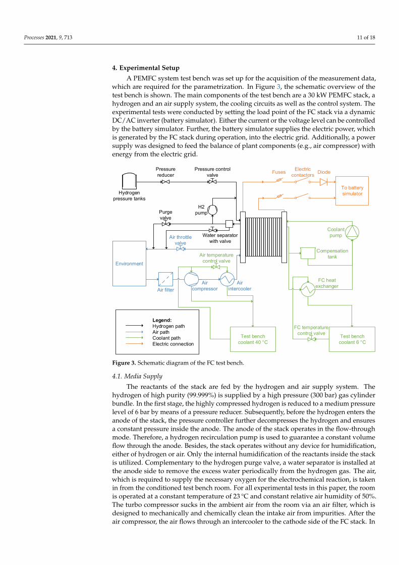
A PEMFC system test bench was set up for the acquisition of the measurement data,which are required for the parametrization. In Figure 3, the schematic overview of thetest bench is shown. The main components of the test bench are a 30 kW PEMFC stack, ahydrogen and an air supply system, the cooling circuits as well as the control system. Theexperimental tests were conducted by setting the load point of the FC stack via a dynamicDC/AC inverter (battery simulator). Either the current or the voltage level can be controlledby the battery simulator. Further, the battery simulator supplies the electric power, whichis generated by the FC stack during operation, into the electric grid. Additionally, a powersupply was designed to feed the balance of plant components (e.g., air compressor) withenergy from the electric grid.

Diode

FC temperature

control valve

FC heat

exchanger

H2

pump

Air

intercooler

Air

compressor

Coolant

pump

Electric

contactors

Compensation

tank

Hydrogen

pressure tanks

Pressure

reducer

Air filter

Fuses

To battery

simulator

Environment

Air temperature

control valve

Air throttle

valve

Water separator

with valve

Purge

valve

Pressure control

valve

Legend:

Hydrogen path

Air path

Coolant path

Electric connection

Test bench

coolant 40 °C

Test bench

coolant 6 °C

Figure 3. Schematic diagram of the FC test bench.

4.1. Media Supply

The reactants of the stack are fed by the hydrogen and air supply system. Thehydrogen of high purity (99.999%) is supplied by a high pressure (300 bar) gas cylinderbundle. In the first stage, the highly compressed hydrogen is reduced to a medium pressurelevel of 6 bar by means of a pressure reducer. Subsequently, before the hydrogen enters theanode of the stack, the pressure controller further decompresses the hydrogen and ensuresa constant pressure inside the anode. The anode of the stack operates in the flow-throughmode. Therefore, a hydrogen recirculation pump is used to guarantee a constant volumeflow through the anode. Besides, the stack operates without any device for humidification,either of hydrogen or air. Only the internal humidification of the reactants inside the stackis utilized. Complementary to the hydrogen purge valve, a water separator is installed atthe anode side to remove the excess water periodically from the hydrogen gas. The air,which is required to supply the necessary oxygen for the electrochemical reaction, is takenin from the conditioned test bench room. For all experimental tests in this paper, the roomis operated at a constant temperature of 23 °C and constant relative air humidity of 50%.The turbo compressor sucks in the ambient air from the room via an air filter, which isdesigned to mechanically and chemically clean the intake air from impurities. After theair compressor, the air flows through an intercooler to the cathode side of the FC stack. In

Processes 2021, 9, 713 12 of 18

order to vary the backpressure of the stack, an electronically controlled air throttle valve isimplemented at the process air exhaust of the FC stack.

4.2. Cooling Circuits

Two different cooling circuits of the test bench environment are used to keep the stack,the air compressor, and the air intercooler at an appropriate temperature. All the othercomponents of the system are designed so that passive cooling is sufficient for them. Thecooling circuit of the FC is thermally connected via a heat exchanger to the 6 °C coolingcircuit of the test bench environment. Moreover, in the cooling circuit of the FC stack, a de-ionized coolant is used. During the operation of the FC stack, the values of the volume flowand the speed of the coolant pump are maintained constant. The 40 °C cooling circuit of thetest bench environment is utilized to cool the air compressor and the intercooler. In order toguarantee a sufficient cooling of the components, flow control valves in the cooling circuitsof the test bench environment are integrated. The target stack coolant inlet temperature is55 °C. The air inlet temperature is kept at a value of 40 °C. The air compressor is suppliedat all times with a constant volume flow of coolant, which is sufficient for the necessarycooling demand.

4.3. Test Bench Control System

Dedicated software was developed in LabVIEW and implemented on a NI Com-pactRio to monitor and control the FC system. With this specific software, the possibilityhas been created to vary each operating parameter of the FC system in an admissible range.Furthermore, with the control system the acquisition of measurement data is realized witha sampling rate of 10 Hz. In order to provide a detailed experimental investigation, avariety of sensors (temperature, pressure, mass flow, voltage, current, and humidity) areinstalled at all relevant positions. Further details with respect to the test bench set up aregiven in [38,39].

4.4. Experimental Tests and Operating Conditions

During the experimental tests, the load point of the stack and the air mass flow, whichis controlled according to the electric current and to a constant air excess ratio of 1.5, werevaried. In order to obtain measurement data under different operating states as well asoperating conditions of the FC system, the load point was adjusted arbitrarily either bysetting the stack voltage or the stack current level in a range, in which a stable operationof the FC is still guaranteed. All other operating parameters of the FC system (targettemperatures, anode pressure setpoint, hydrogen recirculation pump speed, coolant pumpspeed) were kept constant under all load and operating conditions. The standard values ofthe constant operating parameters can be seen in Table 1. For more details regarding theexperimental tests, please refer to Section 5, in which simulated and measured data arepresented and discussed.

Table 1. Constant operating parameters and standard values of the FC system

Operating Parameter Value

Standard stack voltage range 60–120 VDCContinuous stack current 120–400 AAir compressor pressure ratio at 400 A 1.64 (closed throttle valve)Standard excess air ratio (λAir) 1.5Air inlet temperature at cathode 40 °CAnode pressure 1700 mbarH2 pump speed 4000 RPMStack coolant inlet temperature 55 °CAmbient temperature 23 °CAmbient pressure 1000 mbarRelative humidity of ambient air 50%

Processes 2021, 9, 713 13 of 18

5. Results and Discussion5.1. Results

This work proposes a validated two-step parametrization method, and it demon-strates the method by parametrizing the presented model using the measurement dataobtained from the FC test bench. The proceeding is almost identical to the one describedin Section 3.4. The differences are that the measured outputs y∗ now serve as referencedata, the optimizer’s population size is 1000, and the model gets parametrized only once.Therefore all conclusions stated there still hold. Confidentiality agreements do not allowthe publication of the numerical values of the optimized parameters. Figure 4a–d show theparametrization results. Simulating the model with the optimized parameter vector θoptand using the measured inputs u described in Section 4 yields the simulated model outputsy. The figures additionally depict the measured outputs and four model inputs as reference:the mass flow of air mca,in, the FC temperature T, the anode supply manifold pressurepan,sm, and the current I. The parameterized model achieves an R2 value of 93% on average.For validation data, the model reaches an R2 value of 91% on average (see Figure 4e–h),providing the required accuracy for control-oriented applications.

5.2. Discussion

The simulated outputs fit very well. However, the simulated pressures deviate morefrom the measurements than the voltage. The simulated anode exit manifold pressurepan,em (Figure 4c,g) has deviations, which seem to be load-dependent. During low currents,the measured pressure is higher and vice versa. A reason could be the recirculation flow.The recirculation pump runs at a constant speed and should provide a constant flow duringsteady-state. The flow is not measured and is assumed constant in the model. However,steady-state conditions are not always given, especially during purging. Measuring therecirculation flow and adding it as an input to the model could minimize the deviations.The simulated cathode pressures deviate more from the validation data (Figure 4e,f) thanfrom the parametrization data (Figure 4a,b). The maximum deviation is 5%, and a reasonmay be the inflow air temperature, which differs up to 10 °C between the two data sets. In-corporating the inflow air temperature into the model may improve the agreement betweenthe simulated and measured cathode pressures. The model’s simulated voltage response(Figure 4h) replicates the undershooting only in a moderate way for the validation data.One reason could be the underrepresented voltage undershooting in the parametrizationdata (Figure 4d). Using a data set with more often recurring voltage undershooting mayimprove the model’s behavior in this regard. Figure 2b depicts the total information ofthe electrochemical parameters σθel,i . The combined diffusion coefficients, CDca and CDan,have relatively low information. The reason is that the experiments only cover the safeoperating region. The named coefficients determine the limit current and are only wellidentifiable in the unsafe limit current region. According to Figure 2a, the supply andexit manifold volumes (Vca,sm, Vca,em, Van,sm, and Van,em) are not identifiable. The reason isthat only the pressure states needed them, which do not exist anymore. Thus the namedvolumes are not used in the reduced model at all. The named aspects only concern themodel and the experiments, but not the parametrization method itself.

A drawback of the two-step method is that by conducting separate parameter sensi-tivity analyses for the two submodels, slightly different conclusions may follow comparedto the complete model analysis. The reason is that the electrochemical model’s outputcontributes additional information on the thermodynamic parameters. However, the ad-vantage of the reduced solution space dimension compensates for this drawback. Thestated conclusions derived from the FIM only hold in a region near the initial guess ofthe parameters θ0. Hence the FIM is only a local parameter sensitivity analysis. Withanother parameter vector, the conclusions from the newly derived FIM may be different.In general, parameters could be nonsignificant if the excitation is ill-suited (e.g., CDca), it isnot relevant in the model (e.g., Vca,sm), or both. High significancies are interpretable in avice versa manner. As discussed, the parameter identifiability and the derived conclusions

Processes 2021, 9, 713 14 of 18

are strongly dependent on the available measurement data and the model structure. Withthis knowledge, remodeling or a more targeted design of the experiment is possible toimprove identifiability. From the engineering point of view, this information is utilizable todistribute engineering resources efficiently. Focusing on improving the significant parame-ter’s real-world counterparts affects the system outputs substantially more than optimizingthe less significant ones. Optimizing the latter will lead to hardly any changes in theoutput. Furthermore, more measured signals (e.g., anode and cathode outflow relativehumidity, species concentrations, recirculation flow) and more "exciting" system inputswould significantly affect the obtainable results by increasing the Fisher information of theparameters, leading to better parametrization results.

Processes 2021, 9, 713 14 of 19

Processes 2021, 1, 0 14 of 19

0.5

1

1.5

105

0.01

0.02

0.03

0.5

1

1.5

105

330

335

340

0 500 1000 1500

0.8

1

1.2

1.4

1.6105

1.7

1.8

1.9

105

0 500 1000 1500

40

60

80

200

400

600

Parametrization

Time in s

R2 = 99.9%R2 = 98.2%

Pre

ssu

rein

Pa

Mas

sfl

ow

ink

g/

s

(a) pca,sm and mca,in

R2 = 99.4%R2 = −48.2%P

ress

ure

inP

a

Tem

per

atu

rein

K

(b) pca,em and T

R2 = 75.1%

R2 = 9.33%

Pre

ssu

rein

Pa

Pre

ssu

rein

Pa

(c) pan,em and pan,sm

R2 = 98.2%R2 = 72.3%

Vo

ltag

ein

V

Cu

rren

tin

A

(d) U and I

0.5

1

1.5

105

0.01

0.02

0.03

0.5

1

1.5

105

330

335

340

0 100 200 300 400 500

0.8

1

1.2

1.4

105

1.7

1.8

1.9

105

0 100 200 300 400 500

40

60

80

200

400

600

Validation

Simulated y (1-step) Simulated y (2-step) Measured y Measured u

Time in s

R2 = 96.9%

R2 = 92.1%

Pre

ssu

rein

Pa

Mas

sfl

ow

ink

g/

s

(e) pca,sm and mca,in

R2 = 90.3%

R2 = −201%

Pre

ssu

rein

Pa

Tem

per

atu

rein

K

(f) pca,em and T

R2 = 78.5%R2 = −222%

Pre

ssu

rein

Pa

Pre

ssu

rein

Pa

(g) pan,em and pan,sm

R2 = 97.3%R2 = 82.7%

Vo

ltag

ein

V

Cu

rren

tin

A(h) U and I

Figure 4. Plots (a,e): Cathode supply manifold pressure pca,sm (blue, yellow and red), and air mass

flow mca,in (purple). Plots (b,f): Cathode exit manifold pressure pca,em (blue, yellow and red), and

FC temperature T (purple). Plots (c,g): Anode exit manifold pressure pan,em (blue, yellow and red),

and anode supply manifold pressure pan,sm (purple). Plots (d,h): Stack voltage U (blue, yellow and

red), and stack current I (purple). The plots depict parameterization and validation data, respec-

tively, and y denotes output and u input.

5.2. Discussion

The simulated outputs fit very well. However, the simulated pressures deviate more

from the measurements than the voltage. The simulated anode exit manifold pressurepan,em (Figure 4c,g) has deviations, which seem to be load-dependent. During low cur-

rents, the measured pressure is higher and vice versa. A reason could be the recirculation

flow. The recirculation pump runs at a constant speed and should provide a constantflow during steady-state. The flow is not measured and is assumed constant in the model.

However, steady-state conditions are not always given, especially during purging. Mea-suring the recirculation flow and adding it as an input to the model could minimize the

deviations. The simulated cathode pressures deviate more from the validation data (Fig-

ure 4e,f) than from the parametrization data (Figure 4a,b). The maximum deviation is 5%,and a reason may be the inflow air temperature, which differs up to 10 °C between the two

data sets. Incorporating the inflow air temperature into the model may improve the agree-

Figure 4. Plots (a,e): Cathode supply manifold pressure pca,sm (blue, yellow and red), and air massflow mca,in (purple). Plots (b,f): Cathode exit manifold pressure pca,em (blue, yellow and red), and FCtemperature T (purple). Plots (c,g): Anode exit manifold pressure pan,em (blue, yellow and red), andanode supply manifold pressure pan,sm (purple). Plots (d,h): Stack voltage U (blue, yellow and red),and stack current I (purple). The plots depict parameterization and validation data, respectively, andy denotes output and u input.

5.2. Discussion

The simulated outputs fit very well. However, the simulated pressures deviate morefrom the measurements than the voltage. The simulated anode exit manifold pressurepan,em (Figure 4c,g) has deviations, which seem to be load-dependent. During low currents,the measured pressure is higher and vice versa. A reason could be the recirculation flow.The recirculation pump runs at a constant speed and should provide a constant flow duringsteady-state. The flow is not measured and is assumed constant in the model. However,steady-state conditions are not always given, especially during purging. Measuring therecirculation flow and adding it as an input to the model could minimize the deviations.The simulated cathode pressures deviate more from the validation data (Figure 4e,f) thanfrom the parametrization data (Figure 4a,b). The maximum deviation is 5%, and a reasonmay be the inflow air temperature, which differs up to 10 °C between the two data sets. In-corporating the inflow air temperature into the model may improve the agreement betweenthe simulated and measured cathode pressures. The model’s simulated voltage response

Figure 4. Plots (a,e): Cathode supply manifold pressure pca,sm (blue, yellow and red), and air massflow mca,in (purple). Plots (b,f): Cathode exit manifold pressure pca,em (blue, yellow and red), and FCtemperature T (purple). Plots (c,g): Anode exit manifold pressure pan,em (blue, yellow and red), andanode supply manifold pressure pan,sm (purple). Plots (d,h): Stack voltage U (blue, yellow and red),and stack current I (purple). The plots depict parameterization and validation data, respectively, andy denotes output and u input.

Compared to the usual “single-step” approach, the two-step method simplifies theparametrization process significantly by reducing the solution space’s dimension. Asdepicted in Figure 2e, the parameters resulting from a single-step parametrization ofthe entire model (without any further considerations) have a much larger spread, which

Processes 2021, 9, 713 15 of 18

implicitly means a worse fit of the simulation data with the measurements. Figure 4additionally shows the simulation results with parameters obtained from the single-stepapproach. The simulations achieve an average R2 value of 33% for the parametrizationdata and −62% for the validation data, which is much worse than the proposed two-stepmethod (93% and 91%, respectively). However, increasing the optimizer’s population sizeand the number of generations the single-step approach would yield similar results asthe two-step method. By doing so, the single-step approach searches more thoroughlythrough the bigger solution space of the entire model for the optima, but at the expenseof exponentially growing computation time. Therefore, considering limited resourcesand the same optimizer options, the two-step method delivers more accurate results thanthe single-step approach, making the former superior in this case. A comparison of theproposed two-step method with methods consisting of more than two steps is, in this case,not meaningful because this work utilizes pre-existing data. Multiple-step methods [14,18]require appropriately designed experiments, which is usually not the case for pre-existingdata. If the data allows the utilization of a method with more than two steps, then themultiple-step method will likely deliver better results than the two-step method consideringsimilar resources. The fact that the two-step method does not need appropriately designedexperiments compensates for this drawback.

6. Conclusions

This paper presents an efficient two-step parametrization method for FCs. A separa-tion of the model into two submodels decreases the solution space drastically. The methodparametrizes the submodels in two consecutive steps. A parameter sensitivity analysisfurther reduces each sub-solution space, which simplifies the search for the optima. Thiswork demonstrates the efficient method by parametrizing an FC model with measurementsand illustrates the parameter sensitivity analysis’s advantages. The parameterized model’soutputs replicate the validation data excellently.

The parameter sensitivity analysis is a powerful tool to determine the parameters’identifiability with a given model and measurement data. The inverse approach is alsopromising for future research: developing a “design of experiment controller” with a givenmodel to maximize the parameter’s identifiability in real-time.

Author Contributions: Conceptualization, and methodology, Z.P.D. and S.J.; investigation, datacuration, Z.P.D. and C.S.; software and visualization, Z.P.D.; writing–original draft preparation, Z.P.D.and C.S.; writing–review and editing, supervision, and project administration, S.J. All authors haveread and agreed to the published version of the manuscript.

Funding: The research leading to these results has received funding from the Mobility of the Futureprogramme. Mobility of the Future is a research, technology and innovation funding programme ofthe Republic of Austria, Ministry of Climate Action. The Austrian Research Promotion Agency (FFG)has been authorised for the programme management (grant number 871503). The APC was fundedby TU Wien Bibliothek.

Institutional Review Board Statement: Not applicable.

Informed Consent Statement: Not applicable.

Data Availability Statement: Confidentiality agreements do not allow the publication of the datapresented in this study.

Acknowledgments: The computational results presented have been achieved, in part, using theVienna Scientific Cluster (VSC). The authors acknowledge the financial support through Open AccessFunding by TU Wien Bibliothek.

Conflicts of Interest: The authors declare no conflict of interest.

Processes 2021, 9, 713 16 of 18

AbbreviationsThe following abbreviations are used in this manuscript:

FC Fuel cellFIM Fisher information matrixODE Ordinary differential equationPEMFC Polymer electrolyte membrane fuel cellSVD Singular value decomposition

NomenclatureThe following symbols are used in this manuscript:

Subscripts0 Initialact Activationan Anodeatm Atmospherebp Backpressureca Cathodecm Center manifoldel Electrochemicalem Exit manifoldH2 Hydrogenin Inflowleak Leakageliq Liquid waterls Least significantmax Maximummin Minimumms Most significantm MembraneN2 Nitrogennorm NormalizedO2 Oxygenopt Optimizedout Outflowperm Permeabilitypurge Purgereci Recirculationsm Supply manifoldth Thermodynamicvap Vapouri Running index for parametersk Sampling instantl Running index for singular valuesSymbolsα Valve position 1Ψ Output parameter sensitivity matrix R4×nθ

ψ Output parameter sensitivity vector R4×1

Σ Singular value matrix Rnθ×nθ

Σe Prediction error covariance matrix R4×4

θ Parameter vector R25×1

θel Parameter vector of the electrochemical submodel R8×1

θth Parameter vector of the thermodynamic submodel R17×1

ξ State parameter sensitivity vector R9×1

ε2 Membrane conductivity parameter Kγ Threshold 1λAir Excess air ratio 1F Fisher information matrix Rnθ×nθ

f System function of the reduced model R9×1

fnr System function of the non-reduced model R12×1

fth System function of the thermodynamic submodel R9×1

g Output function of the reduced model R4×1

gnr Output function of the non-reduced model R4×1

gth Output function of the thermodynamic submodel R3×1

Qy Output weighting matrix R4×4

Qθ Regularization matrix R25×25

U Left singular vector matrix Rnθ×nθ

u Input vector R8×1

V Right singular vector matrix Rnθ×nθ

Processes 2021, 9, 713 17 of 18

v Right singular vector Rnθ×1

x State vector of the reduced model R9×1

xnr State vector of the non-reduced model R12×1

xth State vector of the thermodynamic submodel R9×1

y Output vector R4×1

y∗ Measured output vector R4×1

yth Output vector of the thermodynamic submodel R3×1

σ Singular valueσθi Total information of parameter θiτ Time constant sθ Parameterϕ Relative humidity 1a Water activity 1CD Combined diffusion coefficient mol/sE Energy Jgel Output function of the electrochemical submodel R1×1

I Current AJ Objective function R1×1

K Intrinsic exchange current parameter A/m2

k Nozzle or mass flow coefficient kg/(s · Pa)kcond Condensation coefficient 1/skevap Evaporation coefficient 1/(s · Pa)m Mass kgnk Number of sample instants (nk + 1) 1nθ Number of parameters 1p Pressure PaR Mass-specific gas constant J/(kg ·K)Rc Ohmic contact resistance ΩT Fuel cell temperature Kt Time sU Voltage VV Volume m3

v Right singular vector componentyel Output of the electrochemical submodel R1×1

References1. Mench, M.M. Fuel Cell Engines; John Wiley & Sons, Inc.: Hoboken, NJ, USA, 2008; pp. 1–515. [CrossRef]2. Napoli, G.; Ferraro, M.; Sergi, F.; Brunaccini, G.; Antonucci, V. Data driven models for a PEM fuel cell stack performance

prediction. Int. J. Hydrog. Energy 2013, 38, 11628–11638. [CrossRef]3. Han, I.S.; Chung, C.B. Performance prediction and analysis of a PEM fuel cell operating on pure oxygen using data-driven

models: A comparison of artificial neural network and support vector machine. Int. J. Hydrog. Energy 2016, 41, 10202–10211.[CrossRef]

4. Wang, Y.; Seo, B.; Wang, B.; Zamel, N.; Jiao, K.; Adroher, X.C. Fundamentals, materials, and machine learning of polymerelectrolyte membrane fuel cell technology. Energy AI 2020, 1, 100014. [CrossRef]

5. Qu, Z.; Aravind, P.; Boksteen, S.; Dekker, N.; Janssen, A.; Woudstra, N.; Verkooijen, A. Three-dimensional computational fluiddynamics modeling of anode-supported planar SOFC. Int. J. Hydrog. Energy 2011, 36, 10209–10220. [CrossRef]

6. Liao, Z.; Wei, L.; Dafalla, A.M.; Suo, Z.; Jiang, F. Numerical study of subfreezing temperature cold start of proton exchangemembrane fuel cells with zigzag-channeled flow field. Int. J. Heat Mass Transf. 2021, 165, 120733. [CrossRef]

7. Sayadian, S.; Ghassemi, M.; Robinson, A.J. Multi-physics simulation of transport phenomena in planar proton-conducting solidoxide fuel cell. J. Power Sources 2021, 481, 228997. [CrossRef]

8. Pukrushpan, J.T.; Stefanopoulou, A.G.; Peng, H. Control of Fuel Cell Power Systems; Advances in Industrial Control; Springer:London, UK, 2004. [CrossRef]

9. Ritzberger, D.; Hametner, C.; Jakubek, S. A Real-Time Dynamic Fuel Cell System Simulation for Model-Based Diagnostics andControl: Validation on Real Driving Data. Energies 2020, 13, 3148. [CrossRef]

10. Ritzberger, D.; Höflinger, J.; Du, Z.P.; Hametner, C.; Jakubek, S. Data-driven parameterization of polymer electrolyte membranefuel cell models via simultaneous local linear structured state space identification. Int. J. Hydrog. Energy 2021, 46, 11878–11893.[CrossRef]

11. Kunusch, C.; Puleston, P.F.; Mayosky, M.A.; Husar, A.P. Control-Oriented Modeling and Experimental Validation of a PEMFCGeneration System. IEEE Trans. Energy Convers. 2011, 26, 851–861. [CrossRef]

12. Nehrir, M.H.; Wang, C. Dynamic Modeling and Simulation of PEM Fuel Cells. In Modeling and Control of Fuel Cells: DistributedGeneration Applications; IEEE: Piscataway, NJ, USA, 2009. [CrossRef]

13. McKay, D.A.; Siegel, J.B.; Ott, W.; Stefanopoulou, A.G. Parameterization and prediction of temporal fuel cell voltage behaviorduring flooding and drying conditions. J. Power Sources 2008, 178, 207–222. [CrossRef]

14. Xu, L.; Fang, C.; Hu, J.; Cheng, S.; Li, J.; Ouyang, M.; Lehnert, W. Parameter extraction of polymer electrolyte membrane fuel cellbased on quasi-dynamic model and periphery signals. Energy 2017, 122, 675–690. [CrossRef]

Processes 2021, 9, 713 18 of 18

15. Müller, E.A.; Stefanopoulou, A.G. Analysis, Modeling, and Validation for the Thermal Dynamics of a Polymer ElectrolyteMembrane Fuel Cell System. J. Fuel Cell Sci. Technol. 2006, 3, 99–110. [CrossRef]

16. Goshtasbi, A.; Chen, J.; Waldecker, J.R.; Hirano, S.; Ersal, T. Effective Parameterization of PEM Fuel Cell Models—Part I:Sensitivity Analysis and Parameter Identifiability. J. Electrochem. Soc. 2020, 167, 044504. [CrossRef]

17. Goshtasbi, A.; Pence, B.L.; Chen, J.; DeBolt, M.A.; Wang, C.; Waldecker, J.R.; Hirano, S.; Ersal, T. Erratum: A Mathematical Modeltoward Real-Time Monitoring of Automotive PEM Fuel Cells. J. Electrochem. Soc. 2020, 167, 049002. [CrossRef]

18. Goshtasbi, A.; Chen, J.; Waldecker, J.R.; Hirano, S.; Ersal, T. Effective Parameterization of PEM Fuel Cell Models—Part II:Robust Parameter Subset Selection, Robust Optimal Experimental Design, and Multi-Step Parameter Identification Algorithm.J. Electrochem. Soc. 2020, 167, 044505. [CrossRef]

19. Nelles, O. Introduction to Optimization. In Nonlinear System Identification; Springer: Berlin/Heidelberg, Germany, 2001. [CrossRef]20. Vrlic, M.; Ritzberger, D.; Jakubek, S. Safe and Efficient Polymer Electrolyte Membrane Fuel Cell Control Using Successive

Linearization Based Model Predictive Control Validated on Real Vehicle Data. Energies 2020, 13, 5353. [CrossRef]21. Böhler, L.; Ritzberger, D.; Hametner, C.; Jakubek, S. Constrained Extended Kalman Filter Design and Application for On-Line

State Estimation of High-Order Polymer Electrolyte Membrane Fuel Cell Systems. Int. J. Hydrog. Energy 2021. [CrossRef]22. Springer, T.E.; Zawodzinski, T.A.; Gottesfeld, S. Polymer Electrolyte Fuel Cell Model. J. Electrochem. Soc. 1991, 138, 2334–2342.

[CrossRef]23. Dutta, S.; Shimpalee, S.; Van Zee, J. Numerical prediction of mass-exchange between cathode and anode channels in a PEM fuel

cell. Int. J. Heat Mass Transf. 2001, 44, 2029–2042. [CrossRef]24. Kravos, A.; Ritzberger, D.; Tavcar, G.; Hametner, C.; Jakubek, S.; Katrasnik, T. Thermodynamically consistent reduced dimen-

sionality electrochemical model for proton exchange membrane fuel cell performance modelling and control. J. Power Sources2020, 454, 227930. [CrossRef]

25. Nijmeijer, H.; van der Schaft, A. Introduction. In Nonlinear Dynamical Control Systems; Springer: New York, NY, USA, 1990.[CrossRef]

26. Lambert, J.D. Stiffness: Linear Stability Theory. In Numerical Methods for Ordinary Differential Systems: The Initial Value Problem;Wiley: New York, NY, USA, 1991.

27. Atkinson, K. Numerical Methods for Ordinary Differential Equations. In An Introduction to Numerical Analysis, 2nd ed.; JohnWiley & Sons: New York, NY, USA, 1989.

28. Ljung, L. Parameter Estimation Methods. In System Identification: Theory for the User, 2nd ed.; Prentice Hall PTR: EnglewoodCliffs, NJ, USA, 1999.

29. Cramér, H. Mathematical Methods of Statistics; Princeton University Press: Princeton, NJ, USA, 1999; Volume 9.30. MathWorks Symbolic Math Toolbox—MATLAB. Available online: https://www.mathworks.com/products/symbolic.html

(accessed on 30 January 2021).31. More, S.; van den Bosch, F.C.; Cacciato, M.; More, A.; Mo, H.; Yang, X. Cosmological constraints from a combination of galaxy

clustering and lensing—II. Fisher matrix analysis. Mon. Not. R. Astron. Soc. 2013, 430, 747–766. [CrossRef]32. Van Doren, J.F.; Douma, S.G.; Van den Hof, P.M.; Jansen, J.D.; Bosgra, O.H. Identifiability: from qualitative analysis to model

structure approximation. IFAC Proc. Vol. 2009, 42, 664–669. [CrossRef]33. Stigter, J.D.; Molenaar, J. A fast algorithm to assess local structural identifiability. Automatica 2015, 58, 118–124. [CrossRef]34. Barz, T.; Körkel, S.; Wozny, G. Nonlinear ill-posed problem analysis in model-based parameter estimation and experimental

design. Comput. Chem. Eng. 2015, 77, 24–42. [CrossRef]35. Eckert, M.; Buchsbaum, G.; Watson, A. Separability of spatiotemporal spectra of image sequences. IEEE Trans. Pattern Anal.

Mach. Intell. 1992, 14, 1210–1213. [CrossRef]36. MathWorks Floating-Point Numbers—MATLAB & Simulink. Available online: https://www.mathworks.com/help/matlab/

matlab_prog/floating-point-numbers.html (accessed on 11 April 2021).37. MathWorks Find Minimum of Function Using Genetic Algorithm—MATLAB ga. Available online: https://www.mathworks.

com/help/gads/ga.html (accessed on 15 February 2021).38. Höflinger, J.; Hofmann, P.; Geringer, B. Experimental PEM-Fuel Cell Range Extender System Operation and Parameter Influence

Analysis. SAE Tech. Pap. 2019. [CrossRef]39. Hoeflinger, J.; Hofmann, P. Air mass flow and pressure optimisation of a PEM fuel cell range extender system. Int. J. Hydrog.

Energy 2020, 45, 29246–29258. [CrossRef]