efficient simulation scheme for spiking neural
TRANSCRIPT

EFFICIENT SIMULATION SCHEME FOR SPIKING NEURAL NETWORKS
Richard R. Carrillo Sánchez
PhD Dissertation Directors:
Eduardo Ros Vidal Eva Martínez Ortigosa Francisco Pelayo Valle

Acknowledgement This work has been supported by the EU projects SpikeFORCE
(IST-2001-35271), SENSOPAC (IST-028056) and the Spanish National Grant (DPI-2004-07032).
Abstract Nearly all neuronal information processing and inter-neuronal
communication in the brain involves action potentials, or spikes, which drive the short-term synaptic dynamics of neurons, but also their long-term dynamics, via synaptic plasticity. In many brain structures, action potential activity is considered to be sparse. This sparseness of activity has been exploited to reduce the computational cost of large-scale network simulations, through the development of "event-driven" simulation schemes. However, existing event-driven simulations schemes use extremely simplified neuronal models. Here, we design, implement and evaluate critically an event-driven algorithm (EDLUT) that uses pre-calculated lookup tables to characterize synaptic and neuronal dynamics. This approach enables the use of more complex (and realistic) neuronal models or data in representing the neurons, while retaining the advantage of high-speed simulation. We demonstrate the method's application for neurons containing exponential synaptic conductances, thereby implementing shunting inhibition, a phenomenon that is critical to cellular computation. We also introduce an improved two-stage event-queue algorithm, which allows the simulations to scale efficiently to highly-connected networks with arbitrary propagation delays. Finally, the scheme readily accommodates implementation of synaptic plasticity mechanisms that depend upon spike timing, enabling future simulations to explore issues of long-term learning and adaptation in large-scale networks.

Index
Figure Index.............................................................................................I Table Index ...........................................................................................III 1 Introduction ....................................................................................1 2 Event-driven simulation based on lookup tables (EDLUT) ...........4
2.1 Introduction ............................................................................4 2.2 Simulator architecture.............................................................6 2.3 Event data structure ................................................................8 2.4 Two-stage spike handling.......................................................9 2.5 Simulation algorithm............................................................11 2.6 Synaptic plasticity ................................................................13
3 Neuron models..............................................................................16 3.1 Integrate-and-fire model with synaptic conductances ..........16
3.1.1 Lookup-table calculation and optimization ..................19 3.2 Integrate-and-fire model with electrical coupling ................25
3.2.1 Introduction ..................................................................25 3.2.2 Event-driven implementation .......................................26
3.3 Cerebellar granule cell model...............................................27 3.3.1 Introduction ..................................................................28 3.3.2 Model description.........................................................29 3.3.3 Definition of model tables ............................................31 3.3.4 Experimental results .....................................................31
3.3.4.1 Subthreshold Rhythmic Oscillations ........................33 3.3.4.2 Bursting behaviour ...................................................35 3.3.4.3 Resonance behaviour................................................37
3.3.5 Accuracy validation......................................................40 3.3.6 Conclusions ..................................................................42
3.4 Hodgkin and Huxley model..................................................42 3.4.1 Accuracy.......................................................................47
4 Simulation accuracy and speed ....................................................49 4.1 Simulation accuracy .............................................................49 4.2 Simulation speed ..................................................................54 4.3 Discussion and conclusions..................................................58
5 Neural population synchronization...............................................60 5.1 Introduction ..........................................................................60 5.2 Results ..................................................................................60
6 Cerebellum model simulation.......................................................63 6.1 Introduction ..........................................................................63 6.2 Cerebellar model...................................................................64

6.3 Neuron models......................................................................67 6.4 Cerebellum model topology .................................................67 6.5 Cerebellar Learning Rules....................................................69 6.6 Robot Platform .....................................................................73 6.7 Experimental Results............................................................76 6.8 Discussion.............................................................................86
7 Discussion and conclusions..........................................................88 8 Publication of results ....................................................................91 Bibliography .........................................................................................95

Figure Index - I -
Figure Index
Figure 2.1: Main structures of the EDLUT simulator. ..........................7 Figure 2.2: The ouput connection list...................................................10 Figure 2.3: Two-stage spike processing ...............................................11 Figure 2.4: Simulation algorithm. ........................................................13 Figure 3.1: Equivalent electrical circuit of a neuron. ...........................16 Figure 3.2: Membrane-potential evolution (synaptic model). ..............18 Figure 3.3: Synaptic-conductance updating table. ...............................20 Figure 3.4: Firing-time prediction table. ..............................................21 Figure 3.5: Membrane-potential updating table. ..................................22 Figure 3.6: Membrane potential depending on ginh coordinates...........24 Figure 3.7: Effect produced by activity through electrical coupling....26 Figure 3.8: Simplified-model obtaining process. .................................29 Figure 3.9: Synaptic activation of the modeled granule cell. ...............33 Figure 3.10: Subthreshold oscillations of the membrane potential. .....34 Figure 3.11: Simulation of subthreshold oscillations with EDLUT.....35 Figure 3.12: Simulation of bursting behaviour with EDLUT. .............36 Figure 3.13: Spike suppression.............................................................37 Figure 3.14: Resonance behaviour. ......................................................39 Figure 3.15: Accuracy comparison.......................................................41 Figure 3.16: Output-spike duplication due to discretization errors. .....44 Figure 3.17: Output-spike omission due to discretization errors. ........45 Figure 3.18: Prevention of erroneous spike omission and duplication.46 Figure 3.19: Event-driven simulation of an H&H model neuron.........48 Figure 4.1: Single-neuron simulation. ..................................................50 Figure 4.2: Simulation error depending on synaptic weights...............52 Figure 4.3: Simulation error depending on table size...........................53 Figure 4.4: Output spike trains for different table sizes. ......................54 Figure 4.5: Computation time...............................................................55 Figure 5.1: Neural-population synchronization histograms. ................62 Figure 6.1: Encoding of mossy fibers...................................................66 Figure 6.2: Cerebellum model diagram................................................68 Figure 6.3: Inferior-olive probabilistic encoding of the error. .............70 Figure 6.4: Spike Time Dependent Plasticity.......................................71 Figure 6.5: Input current to inferior olivary cells. ................................73 Figure 6.6: Experimental robot platform..............................................74 Figure 6.7: Complete hardware system. ...............................................75 Figure 6.8: Software architecture. ........................................................76

Figure Index - II -
Figure 6.9: Diagram of the arm-movement control system. ................78 Figure 6.10: Target reaching experiments............................................81 Figure 6.11: Target reaching example..................................................82 Figure 6.12: Corrective torques applied by the cerebellum..................82 Figure 6.13: Arm in the sand-pool context...........................................83 Figure 6.14: Arm trayectory when learning in different contexts. .......84 Figure 6.15: Temporal adaptation. .......................................................85

Table Index - III -
Table Index
Table 3.1: Synaptic characteristics (cerebellar granule cell). ...............19 Table 3.2: Hodgkin and Huxley (1952) model equations. ...................43 Table 4.1: Performance evaluation of different methods. ....................57 Table 6.1: Connectivity table of the cerebellar cells. ...........................68

Introduction - 1 -
1 Introduction
Most natural neurons communicate by means of individual spikes. Information is encoded and transmitted in these spikes, and nearly all of the computation is driven by these events. This includes both short-term computation (synaptic integration) and long-term adaptation (synaptic plasticity). In many brain regions, spiking activity is considered to be sparse. This, coupled with the computational cost of large-scale network simulations, has given rise to the “event-driven" simulation schemes. In these approaches, instead of iteratively calculating all the neuron variables along the time dimension, the neuronal state is only updated when a new event is received.
Various procedures have been proposed to update the neuronal state in this discontinuous way (Watts, 1994; Delorme et al, 1999; Delorme & Thorpe, 2003; Mattia and Del Giudice, 2000; Reutimann, et al, 2003). In the most widespread family of methods, the neuron's state variable (membrane potential) is updated according to a simple recurrence relation that can be described in closed form. The relation is applied upon reception of each spike and depends only upon the membrane potential following the previous spike, the time elapsed, and the nature of the input (strength, sign).
),,( ,, JtVfV ttmtm ∆= ∆− Eq. ( 1.1 )
where Vm is the membrane potential, ∆t is elapsed time (since the last spike) and J represents the effect of the input (excitatory or inhibitory weight).
This method can describe integrate-and-fire neurons and is used, for instance, in SpikeNET (Delorme et al, 1999, Delorme & Thorpe, 2003). Such algorithms can include both additive and multiplicative synapses (i.e. synaptic conductances), as well as short-term and long-term synaptic plasticity. However, the algorithms are restricted to synaptic mechanisms whose effects are instantaneous and to neuronal models which can only spike immediately upon receiving input. These

Introduction - 2 -
conditions obviously restrict the complexity (realism) of the neuronal and synaptic models that can be used.
Implementing more complex neuronal dynamics in event-driven schemes is not straightforward. As discussed by Mattia and Del Giudice (2000), incorporating more complex models requires extending the event-driven framework to handle predicted spikes that can be modified if intervening inputs are received; the authors propose one approach to this issue. However, in order to preserve the benefits of computational speed, it must, in addition, be possible to update the neuron state variable(s) discontinuously and also predict when future spikes would occur (in the absence of further input). Except for the simplest neuron models, these are non-trivial calculations, and only partial solutions to these problems exist. Makino (2003) proposed an efficient Newton-Raphson approach to predicting threshold crossings in Spike-Response Model neurons. However, the method does not help in calculating the neuron's state variables discontinuously, and has only been applied to spike-response models involving sums of exponentials or trigonometric functions. As we shall show below, it is sometimes difficult to represent neuronal models effectively in this form. A standard optimisation in high-performance code is to replace costly function evaluations with lookup tables of pre-calculated function values. This is the approach that was adopted by Reutimann et al (2003) in order to simulate the effect of large numbers of random synaptic inputs. They replaced the on-line solution of a partial differential equation with a simple consultation of a pre-calculated table.
Motivated by the need to simulate a large network of 'realistic' neurons (explained below), we decided to carry the lookup table approach to its logical extreme: to characterise all neuron dynamics off-line, enabling the event-driven simulation to proceed using only table lookups, avoiding all function evaluations. We term this method EDLUT (for Event-Driven Lookup Table). As mentioned by Reutimann et al (2003), the lookup tables required for this approach can become unmanageably large when the model complexity requires more than a handful of state variables. Although we have found no way to avoid this scaling issue, we have been able to optimise the calculation and storage of the table data such that quite rich and complex neuronal models can nevertheless be effectively simulated in this way.

Introduction - 3 -
The initial motivation for these simulations was a large-scale real-time model of the cerebellum. This structure contains very large numbers of granule cells, which are thought to be only sparsely active. An event-driven scheme would therefore offer a significant performance benefit. However, an important feature of the cellular computations of cerebellar granule cells is reported to be shunting inhibition (Mitchell & Silver, 2003), which requires non-instantaneous synaptic conductances. These cannot be readily represented in any of the event-driven schemes based upon simple recurrence relations. For this reason we chose to implement the EDLUT method. Note that non-instantaneous conductances may be important generally, not just in the cerebellum (Eckhorn et al, 1988; Eckhorn et al, 1990).
The axons of granule cells, the parallel fibres, traverse large numbers of Purkinje cells sequentially, giving rise to a continuum of propagation delays. This spread of propagation delays has long been hypothesised to underlie the precise timing abilities attributed to the cerebellum (Braitenberg & Atwood, 1958). Large divergences and arbitrary delays are features of many other brain regions, and it has been shown that propagation/synaptic delays are critical parameters in network oscillations (Brunel & Hakim, 1999). Previous implementations of event queues were not optimised for handling large synaptic divergences with arbitrary delays. Mattia & Del Giudice (2000) implemented distinct fixed-time event queues (i.e., one per delay), which, though optimally quick, would become quite cumbersome to manage when large numbers of distinct delays are required by the network topology. Reutimann et al (2003) and Makino (2003) used a single ordered event structure in which all spikes are considered independent. However, for neurons with large synaptic divergences, unnecessary operations are performed on this structure, since the arrival order of spikes emitted by a given neuron is known. We introduce a two-stage event queue that exploits this knowledge to handle efficiently large synaptic divergences with arbitrary delays.
We demonstrate our implementation of the EDLUT method for models of single-compartment neurons receiving exponential synaptic conductances (with different time constants for excitation and inhibition). In particular, we describe how to calculate and optimize the lookup tables, and the implementation of the two-stage event queue.

Event-driven simulation based on lookup tables (EDLUT) - 4 -
2 Event-driven simulation based on lookup tables (EDLUT)
2.1 Introduction
Recent research projects are modelling neural networks based on specific brain areas. Realistic neural simulators are required in order to evaluate the proposed network models. Some of these models (e.g. related with robot control or image processing (Van Rullen et al, 1998; Philipona et al, 2004) are intended to interface with the real world, requiring real-time neural simulations. This kind of experiments demands efficient software able to simulate large neural populations with moderated computational power consumption.
Traditionally, neural simulations have been based on discrete time step (synchronous) methods (Bower et al, 1998; Delorme et al, 2003). In these simulations, the state variables of each neuron are updated every time step, according to the current inputs and the previous values of these variables. The differential expressions describing the neural model dynamics are usually computed with numerical integration methods such as Euler or Runge-Kutta. The precision of the numerical integration of these variables depends on the time step discretization. Short time steps are required in order to achieve acceptable precision, which means considerable computational power consumption by each neuron. Thus, simulating large neural population with adequate precision and detailed models using these methods is not feasible in real-time.
One alternative to avoid this problem is the use of event-driven simulators (also known as discrete-event simulators). Most natural network communication is done by means of spikes (action potentials) which are short and considerably sparse in time (not very frequent) events. If the state evolution of a neuron between these spikes is deterministic or the probability of all the target states is known, the number of neural state updates could be reduced, accumulating the entire computational load in the instants in which the spikes are produced or received by a neuron (Watts, 1994; Mattia et al, 2000).

Event-driven simulation based on lookup tables (EDLUT) - 5 -
Mattia and Guidice (Mattia et al, 2000) proposed an event-driven scheme that included dynamical synapses. Reutimann et al extended this approach to include neuron models with stochastic dynamics.
Makino (Makino, 2003) developed an event-driven simulator which uses efficient numerical methods to calculate the neural states evolution from one discrete computed step to the next one. More concretely, the main contribution of this work is the development of an efficient strategy to calculate the delayed firing times that uses the linear envelopes of the state variable of the neuron to partition the simulated time. Contrary to this approach, we avoid this complex calculation by off-line characterization of the firing behaviour of the cell.
Recently, Reutimann et al (2003) proposed the use of pre-calculated lookup tables to speed up simulations to avoid on-line numerical calculations. We adopt this strategy in our event-driven simulator. In this previous approach the precalculated tables are used to store probability density distributions. In our approach, the entire cell model is computed off-line, and its behaviour is compiled into characterization tables. Since the cell model is computed off-line, we are able to simulate models of different complexities (with a constraint on the number of parameters defining cell dynamics).
The main innovation with respect to previous similar approaches (Watts, 1994; Mattia et al, 2000), is the use of characterization tables to describe the cell dynamics between input spikes. A priori, this fact removes the need for many of the simplifying assumptions necessary when the neural models are computed following simple expressions to achieve high computational efficiency.
Another important aspect, that has been included, is the synaptic temporal dynamics (i.e. the gradual injection/extraction of charge). The synaptic conductance evolution due to an input spike is not computed as an instantaneous jump, but as a gradual function. This is important in the study of neural population synchronization processes (Eckhorn et al, 1988; Eckhorn et al, 1990). The inclusion of temporal dynamics forces the implementation of a prediction and validation strategy, since the output spikes will not be coincident with the input events (variable firing delay). This introduces some more complexity in the simulation algorithm.
Event-driven simulation based on lookup tables (EDLUT) - 6 -
2.2 Simulator architecture
The EDLUT simulation scheme is based on the structures shown in Figure 2.1, simulation is initialised by defining the network and its interconnections (including latency information), giving rise to the Neuron list and Interconnection list structures. In addition, several lookup tables which completely characterise the neuronal and synaptic dynamics are calculated: i) the exponential decay of the synaptic conductances; ii) a table that can be used to predict if and when the next spike of a cell would be emitted, in the absence of further input; and iii) a table defining the membrane potential (Vm) as a function of the combination of state variables at a given point in the past (in our simulations, this table gives Vm as a function of the synaptic conductances and the membrane potential, all at the time of the last event, and the time elapsed since that last event). If different neuron types are included in the network, they will require their own characterization lookup tables with different parameters defining their specific dynamics. Each neuron in the network stores its state variables at the time of the last event, as well as the time of that event. If short or long-term synaptic dynamics are to be modelled, additional state variables are stored per neuron or per synapse.
Event-driven simulation based on lookup tables (EDLUT) - 7 -
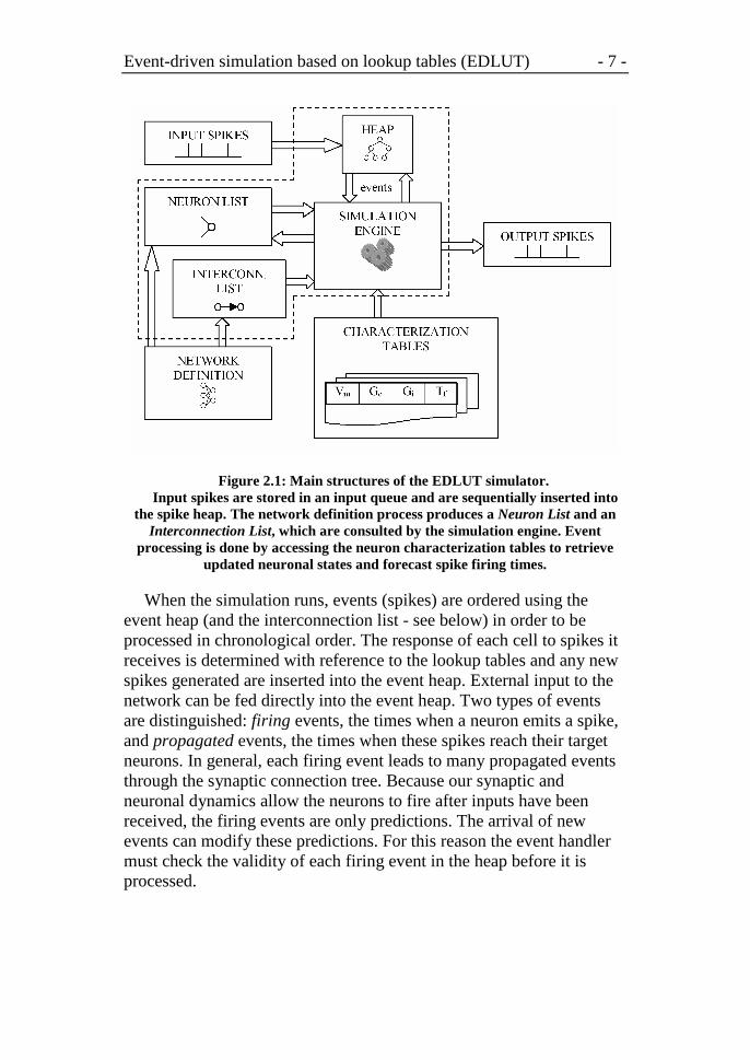
Figure 2.1: Main structures of the EDLUT simulator. Input spikes are stored in an input queue and are sequentially inserted into
the spike heap. The network definition process produces a Neuron List and an Interconnection List, which are consulted by the simulation engine. Event
processing is done by accessing the neuron characterization tables to retrieve updated neuronal states and forecast spike firing times.
When the simulation runs, events (spikes) are ordered using the event heap (and the interconnection list - see below) in order to be processed in chronological order. The response of each cell to spikes it receives is determined with reference to the lookup tables and any new spikes generated are inserted into the event heap. External input to the network can be fed directly into the event heap. Two types of events are distinguished: firing events, the times when a neuron emits a spike, and propagated events, the times when these spikes reach their target neurons. In general, each firing event leads to many propagated events through the synaptic connection tree. Because our synaptic and neuronal dynamics allow the neurons to fire after inputs have been received, the firing events are only predictions. The arrival of new events can modify these predictions. For this reason the event handler must check the validity of each firing event in the heap before it is processed.

Event-driven simulation based on lookup tables (EDLUT) - 8 -
2.3 Event data structure
Events (spikes) must be treated in chronological order in order to preserve the causality of the simulation. The event handling algorithm must therefore be capable of maintaining the temporal order of spikes. To fulfil this, a spike data structure that functions as an interface between the source neuron events and target neurons can be used.
If we need to deal with only a fixed number of neuron-connection delays, there is the possibility that a fixed structure (called a Synaptic Matrix) is used for storing synaptic delays (Mattia & Del Guidice, 2000).
In contrast, our simulations needed to support arbitrary synaptic delays. Complex data structures, such as “balanced trees”, can be used for this purpose, offering good performance for both sorted and random-order input streams. To prevent performance degradation, they optimize their structure after each insertion or deletion. However, this rebalancing process adds more complexity and additional computational overhead (Karlton et al, 1976). Insertion and deletion of elements in these structures have a computational cost of O(log(N)), where N is the number of events in the structure.
Another candidate data structure is the “skip list” (Pugh, 1990), but in this instance the cost of the worst case may not be O(log(N)) because the insertion of an input stream can produce an unbalanced structure. Consequently, the search time for a new insertion may be longer than in the balanced trees. This structure offers optimal performance in searching specific elements. However, this is not needed in our computation scheme as we only need to extract the first element, i.e., the next spike.
Finally, the “heap data structure” (priority queue) (Aho et al, 1974; Chowdhury & Kaykobad, 2001; Cormen et al, 1990) offers a stable computational cost of O(log(N)) in inserting and deleting elements. This is the best option as it does not require more memory resources than the stored data. This is because it can be implemented as an array, while the “balanced trees” and “skip lists” need further pointers or additional memory resources.

Event-driven simulation based on lookup tables (EDLUT) - 9 -
For all of these methods, the basic operation of inserting an event costs roughly O(log(N)), where N is the number of events in the event data structure. Clearly, the smaller the data structure, the less time such insertions will take. We explain in the next subsection the two-stage event handling process we have implemented in order to minimize event heap size while allowing arbitrary divergences and latencies. Compared to a method using a single event data structure, we would expect the event insertions to be O(log(c)) quicker, where c is the average divergence (connectivity).
2.4 Two-stage spike handling
The algorithm efficiency of event-driven schemes depends on the size of the event data structure, so performance will be optimal under conditions that limit load (low connectivity, low activity). However, large synaptic divergences (with many different propagation delays) are an important feature of most brain regions. Previous implementations of event-driven schemes have used a single event generation per neuron firing, (Reutimann et al, 2003; Makino, 2003). However, treating each neuron firing as a single event leads the event data structure to become larger than necessary. Since the order of spike arrival to target neurons is always known (it depends on the connection delay defined in Interconnection list), we know which event has to be processed first.
We have designed an algorithm that exploits this knowledge, by using a multi-stage spike handling process:
Each spike transmitted between two cells is represented internally by two events. The first one (the firing event) is marked with the time instant when the source neuron fires the spike. The second one (the propagated event) is marked with the time instant when the spike reaches the target neuron. Most neurons have large synaptic divergences. In these cases, when a neuron fires, the simulation scheme inserts into the event heap only one event in each stage, instead of one per output connection.
The output connection list of each neuron (which indicates its target cells) is sorted by propagation delay, see Figure 2.2. When a source neuron fires, only the event corresponding to the lowest-latency

Event-driven simulation based on lookup tables (EDLUT) - 10 -
connection is inserted into the spike heap. This event is linked to the other output spikes of this source neuron. When the first spike is processed and removed from the heap, the next event in the output connection list is inserted into the spike heap, taking into account the connection delay. Since the output connection list of each neuron is sorted by latency, the next connection carrying a spike can easily be found. This process is repeated until the last event in the list is processed. In this way, the system can handle large connection divergences efficiently.
Figure 2.2: The ouput connection list. The output connection list of each neuron is sorted by the connection delay,
so the next connection carrying a spike can easily be found.
In Figure 2.3 we compare the use of one and two-stage event handling within our simulation scheme. Even though event heap operations only represent part of the total computation time, there is a clear benefit to using the two-stage process. For divergences of up to 10000 - typical for recurrent cortical networks - a better than 2-fold improvement of total computation time is observed.

Event-driven simulation based on lookup tables (EDLUT) - 11 -
Figure 2.3: Two-stage spike processing Total computation time for processing an event (top) and size of the event
heap (bottom) for one-stage (dashed plot) and two-stage (continuous plot) as functions of synaptic divergence.
2.5 Simulation algorithm
The basic computation scheme consists of a processing loop, in each iteration of which the next event (i.e., with the shortest latency) is taken from the spike heap. This event is extracted from the spike heap structure, the target neuron variables are updated (in the neuron list structure), and, if the affected neurons generate them, new events are inserted into the spike heap. Also, if the processed event is a propagated event, the next spike from the output connection list of the neuron is inserted into the heap. This computation scheme is summarized in Figure 2.4. It should be noted that events are inserted into the heap in correct temporal sequence, but only the spike with the shortest latency is ever extracted.

Event-driven simulation based on lookup tables (EDLUT) - 12 -
As our neuronal model allows delayed firing (after inputs), the algorithm must cope with the fact that predicted firing times may be modified –or even deleted– by intervening posterior inputs.
Each neuron stores two time variables. One indicates the time the neuron was last updated. This happens upon reception of each input. As described in Figure 2.4, when a neuron is affected by an event, the time label of this neuron is updated to tsim if it is an input spike (propagated event) or to tsim+trefrac if it is an output spike (firing event), to prevent it from firing again during the refractory period. This is important because when the characterization tables are consulted the time label indicates the time that has elapsed since the last update. The other time label maintains the up-to-date firing time prediction. This is used to check the validity of events extracted from the central event heap.
Events that are superseded by intervening inputs in the neuron concerned are left in the event heap; they are discarded upon extraction. Since if they are invalid, their firing-time-prediction variable stored in the neuron does not match the current simulation time (this is checked when the event is being processed).

Event-driven simulation based on lookup tables (EDLUT) - 13 -
While tsim<tend { Extract the event with a shortest latency in the spike heap
If it is a firing event
If it is still a valid event and the neuron is not under a refractory period
Update the neuron state (e.g. Vm, gexc, ginh) to the post-firing state Prevent this neuron from firing during the refractory period by updating the neuron time label to tsim+trefrac) Predict if the source neuron will fire again with the current neuron state If the neuron will fire:
Insert a new firing event into the spike heap
Insert the propagated event with the shortest latency (looking at the output connection list)
If it is a propagated event Update the target neuron state (e.g. Vm, gexc, ginh), before the event is computed Modify the conductances (gexc, ginh) using the connection weight (Gexc,i, Ginh,i) for the new spike Update the neuron time label to tsim Predict if the target neuron will fire If it fires
Insert the firing event into the spike heap with the predicted time
Insert only the next propagated event with the next shortest latency (looking at the output connection delay table)
}
Figure 2.4: Simulation algorithm.
This pseudo-code describes the simulation engine. It processes all the events of the spike heap in chronological order.
2.6 Synaptic plasticity
We have implemented Hebbian-like (Hebb, 1949) spike-driven learning mechanisms (spike-timing-dependent plasticity, STDP). The

Event-driven simulation based on lookup tables (EDLUT) - 14 -
implementation of such leaning rules is suitable because the simulation scheme is based on the time labels of the different events. Spike-time-dependent learning rules require comparison of the times of pre-synaptic spikes (propagated events) with post-synaptic spikes (firing event). In principle, this requires the trace of the processed pre-synaptic spikes during a time interval to be kept in order for them to be accessible if post-synaptic spikes occur. Different definite expressions can be used for the learning rule (Gerstner & Kistler, 2002). The weight change function has been approximated with exponential expressions; Eq. ( 2.1 ) to accommodate the experimental results of Bi and Poo (1998). The computation of this learning rule, by means of exponential terms, facilitates its implementation in a recursive way, avoiding the need to keep track of previous spikes.
>
<=
−
0
0)(
sifea
sifeasf sb
post
sbpre
post
pre
Eq. ( 2.1 )
Where s represents the temporal delay between the post-synaptic spike and the pre-synaptic one (s=tpost-tpre). The aim function (Bi & Poo, 1998) can be calculated with Eq. ( 2.1 ) using the following parameters (apre=0.935, bpre= -0.075, apost= -0.326, bpost= -0.036). They have been approximated using the Trust-region method (Conn et al 2000).
The learning rules are applied each time a cell both receives and fires a spike. Each time a spike from cell i reaches a neuron j, the connection weight (wij) is changed according to Eq. ( 2.2 ), taking into account the time since the last action potential (AP) in the post-synaptic neuron. This time is represented by s in Eq. ( 2.1 ).
)(sfww
where
www
ijij
ijijij
=∆
∆+←
Eq. ( 2.2 )
Other post-synaptic spikes are not taken into account for the sake of simplicity, but they can be included if necessary.
Each time cell j fires a spike, the learning rule of Eq. ( 2.3 ) is applied, taking into account all the pre-synaptic spikes received in a certain interval.

Event-driven simulation based on lookup tables (EDLUT) - 15 -
∑=∆
∆+←
kkijij
ijijij
sfww
where
www
)(
Eq. ( 2.3 )
In order to avoid keeping track of all the pre-synaptic spikes during the learning window, we can rearrange the sum of Eq. ( 2.3 ), since the learning rule can be expressed in terms of exponentials; Eq. ( 2.1 ).
Each time the neuron fires a spike, the learning rule is applied in each input connection, taking into account the previous spikes received through these inputs. Therefore, each weight changes according to Eq. ( 2.4 ).
( )
+=+← ∑∑
==
N
k
sbpreij
N
kkijijij
kpreeawsfwww11
1 Eq. ( 2.4 )
Where k is iterated over all N pre-synaptic spikes from cell i received by the neuron j in a time window. This expression can be rearranged as follows:
( )( )( )( )( )( )( )Npreprepreprepre
Npreprepre
sbsbsbsbsbpreijijij
sbsbsbpreijijij
eeeawww
eeeawww
+++ +++++←
++++←...1211
21
...1
1...11 Eq. ( 2.5 )
This expression; Eq. ( 2.5 ) can be calculated recursively accumulating all the multiplicative terms in an intermediate variable Aij, as indicated in Eq. ( 2.6 ). s is the time difference between the action potential of cell j and the last pre-synaptic spike received from cell i.
sbijij
preeAA +←1 Eq. ( 2.6 )
The learning rule is applied recursively as indicated in Eq. ( 2.7 ), incorporating the last pre-synaptic spike. Note that the term Aij accumulates the effect of all previous pre-synaptic spikes.
( )ijsb
preijij
ijijij
Aeaww
where
www
pre=∆
∆+←
Eq. ( 2.7 )

Neuron models - 16 -
3 Neuron models
3.1 Integrate-and-fire model with synaptic conductances
In this model, neurons are single compartments receiving exponential excitatory and inhibitory synaptic conductances with different time constants. The basic electrical components of the neuron model are shown in Figure 2.1. The neuron is described by the following parameters: (1) membrane capacitance, Cm, (2) the reversal potentials of the synaptic conductances, Eexc and Einh, (3) the time constants of the synaptic conductances, τexc and τinh, and (4) the resting conductance and its reversal potential, grest and Erest, respectively. The membrane time constant is defined as τm = Cm/grest. The neuron state variables are the membrane potential (Vm), the excitatory conductance (gexc) and the inhibitory conductance (ginh). The synaptic conductances gexc and ginh depend on the inputs received from the excitatory and inhibitory synapses, respectively.
Figure 3.1: Equivalent electrical circuit of a neuron.

Neuron models - 17 -
gexc and ginh are the excitatory and inhibitory synaptic conductances, while grest is the resting conductance, which returns the membrane potential to its resting
state (Erest) in the absence of input stimuli.
The decision was made to model synaptic conductances as exponentials:
( ) ( )
≥⋅<
= −−0
0
,
,00 tteG
tttg
excttexc
exc τ
( ) ( )
≥⋅<
= −−0
0
,
,00 tteG
tttg
inhttinh
inh τ
Eq. ( 3.1 )
where Gexc and Ginh represent the peak individual synaptic conductances and gexc and ginh represent the total synaptic conductance of the neuron. This exponential representation has numerous advantages. Firstly, it is an effective representation of realistic synaptic conductances. Thus, the improvement in accuracy from the next most complex representation, a double-exponential function, is hardly worthwhile when considering the membrane potential waveform (See Figure 3.2).

Neuron models - 18 -
Figure 3.2: Membrane-potential evolution (synaptic model). A post-synaptic neuron receives two consecutive input spikes (top). The evolution of the synaptic conductance is the middle plot. The two EPSPs caused by the two
input spikes are shown in the bottom plot. In the solid line plots, the synaptic conductance transient is represented by a double-exponential expression (one
exponential for the rising phase, one for the decay phase). In the dashed line plot, the synaptic conductance is approximated by a single-exponential expression. The EPSPs produced with the different conductance waveforms are almost
identical.
Secondly, the exponential conductance requires only a single state variable, because different synaptic inputs can simply be summed recursively when updating the total conductance:
)()( _)(
, tgeGtg previousexctt
jexcexcikepreviousspkecurrentspi −−+= Eq. ( 3.2 )
(Gexc,j is the weight of synapse j; a similar relation holds for inhibitory synapses). Most other representations would require additional state variables and/or storage of spike time lists, so the exponential representation is particularly efficient in terms of memory usage.
In our simulations, the synaptic parameters have been chosen to represent excitatory AMPA-receptor-mediated conductances and inhibitory GABAergic conductances of cerebellar granule cells (Silver et al, 1996; Nusser et al, 1997; Tia et al, 1996; Rossi & Hamann, 1998).

Neuron models - 19 -
These are summarized in Table 3.1. Note that different synaptic connections in different cells might have quite distinct parameters: extreme examples in the cerebellum include the climbing fibre input to Purkinje cells and the mossy fibre input to unipolar brush cell synapses.
Max. Conductance (Gexc_max) nS
Time Constant (τexc) ms
Reversal potential (Eexc)
mV
Excitatory Synapse
0-7.5 0.5 0 Max.
Conductance (Ginh_max) nS
Time Constant (τinh) ms
Reversal potential (Einh)
mV
Inhibitory Synapse
0-29.8 10 -80 Table 3.1: Synaptic characteristics (cerebellar granule cell).
The first column is an estimation of the maximum cell conductance (summed over all synapses on the cell). The conductances of individual synapses (Gexc and Ginh) are not included in this table as they depend on the connection strengths
and are therefore provided through the network definition process and synaptic plasticity.
The differential equation; Eq. ( 3.3 ) describes the membrane potential evolution (for t≥t0) in terms of the excitatory and inhibitory conductances at t0, combined with the resting conductance.
( ) ( ) ( ) ( ) ( ) ( ) ( )mrestrestminhtt
inhmexctt
excm
m VEGVEetgVEetgdt
dVC inhexc −+−+−= −−−− ττ 00
00
Eq. ( 3.3 )
where the conductances gexc(t0) and ginh(t0) integrate all the contributions received through individual synapses. Each time a new spike is received, the total excitatory and inhibitory conductances are updated using Eq. ( 3.2 ). Eq. ( 3.3 ) is amenable to numerical integration. In this way, we can calculate Vm, gexc, ginh and firing time tf for given time intervals after the previous input spike. tf is the time when the membrane potential would reach the firing threshold (Vth) in the absence of further stimuli (if indeed the neuron would fire).
3.1.1 Lookup-table calculation and optimization
The expressions given in the previous subsection are used to generate the lookup tables that characterize each cell type, with each cell model requiring four tables:

Neuron models - 20 -
- Conductances: gexc(∆t) and ginh(∆t) are one-dimensional tables that contain the fractional conductance values as functions of the time ∆t elapsed since the previous spike.
- Firing time: Tf(Vm,t0,gexc,t0,ginh,t0) is a three-dimensional table representing the firing time prediction in the absence of further stimuli.
- Membrane potential: Vm(Vm,t0,gexc,t0,ginh,t0,∆t) is a four-dimensional table that stores the membrane potential as a function of the variables at the last time that the neuron state was updated and the elapsed time ∆t.
Figure 3.3, Figure 3.4 and Figure 3.5 show some examples of the contents of these tables for a model of the cerebellar granule cell with the following parameters: Cm=2pF, τexc=0.5ms, τinh=10ms, grest=0.2nS, Eexc=0V, Einh=-80mV, Erest=-70mV and Vth=-70mV.
Figure 3.3: Synaptic-conductance updating table. fg(∆t); the percentage conductance remaining after a time (∆t) has elapsed since the last spike was received. This is a lookup table for the normalised exponential function. The time constant of the excitatory synaptic conductance gexc (shown
here) was 0.5 ms and for ginh(t), 10 ms. Since the curve exhibits no abrupt changes in the time interval [0, 0.0375] seconds, only 64 values were used.

Neuron models - 21 -
Figure 3.4: Firing-time prediction table. Firing time ( tf) plotted against gexc and initial V m. tf decreases as the excitatory
conductance increases and as Vm,t0 approaches threshold. ginh = 0.

Neuron models - 22 -
Figure 3.5: Membrane-potential updating table. Membrane potential Vm(Vm,t0, gexc,t0, ginh,t0, ∆t) plotted as a function of (A) Vm,t0
and ∆t (gexc = ginh = 0); (B) Gexc,t0 and ∆t (ginh = 0, Vm,t0 = Erest = -70mV). The zoom in the ∆t axis of plot (b) highlights the fact that the membrane potential change
after receiving a spike is not instantaneous.
The sizes of the lookup tables do not significantly affect the processing speed, assuming they reside in main memory (i.e., they are too large for processor cache but small enough not be swapped to disk). However, their size and structure obviously influence the accuracy with which the neural characteristic functions are represented. The achievable table sizes (in particular the membrane potential table) are limited by memory resources. However, it is possible to optimize storage requirements by adapting the way in which their various dimensions are sampled. Such optimization can be quite effective, because some of the table functions only change rapidly over small domains. We evaluate two strategies: multi-resolution sampling and logarithmic compression along certain axes. Different approaches for the membrane potential function Vm(Vm,t0, gexc,t0, ginh,t0, ∆t), the largest table, with respect to the inhibitory conductance (ginh,t0) are illustrated in Figure 3.6. It can be seen that a logarithmic sampling strategy in the conductance dimensions is an effective choice for improving the accuracy of the representation of neural dynamics. For the following simulations we have used logarithmic sampling in the ginh and gexc dimensions of the Vm table (as illustrated in Figure 3.6 C).

Neuron models - 23 -

Neuron models - 24 -
Figure 3.6: Membrane potential depending on ginh coordinates. Each panel shows 16 Vm relaxations with different values of ginh,t0. The sampled
conductance interval is ginh,t0 ∈∈∈∈ [0,20]nS. A) Linear approach: [0,20]nS was sampled with a constant inter-sample distance. B) Multi-resolution approach: two intervals [0,0.35]nS and [0.4,20]nS with eight traces each were used. C)
Logarithmic approach: ginh,t0 was sampled logarithmically.
Storage requirements and calculation time are dominated by the largest table, that for Vm. We shall show in the next chapter that a table containing about a million data points (dimension sizes: ∆t = 64, gexc = 16, ginh = 16, Vm,to = 64) gives reasonable accuracy. In order to populate this table we solve numerically Eq. ( 3.3 ). This was done using a Runge-Kutta method with Richardson extrapolation and adaptive step size control. On a 1.8GHz Pentium computer, calculation of this table takes about 12s. The firing time table had the same dimensions for gexc, ginh, and Vm,to. As stated previously, the individual conductance lookup tables had 64 elements each.
In principle these tables could also be based upon electrophysiological recordings. Since one of the dimensions of the tables is the time, the experimenter would only need to set up the initial values of gexc, ginh and Vm and then record the membrane potential evolution following this initial condition. With our 'standard' table size, the experimenter would need to measure neuronal behaviour for 64 x 16 x 16 (Gexc, Ginh, Vm) triplets. If neural behaviour is recorded in sweeps of 0.5 seconds (at least 10 membrane time constants), only 136 minutes of recording would be required, which is feasible (see below

Neuron models - 25 -
for ways to optimize these recordings). Characterization tables of higher resolution would require longer recording times, but such tables could be built up by pooling/averaging recordings from several cells. Moreover, since the membrane potential functions are quite smooth, interpolation techniques would allow the use of smaller, easier to compile, tables.
In order to control the synaptic conductances (gexc and ginh), it would be necessary to use the dynamic clamp method (Prinz, Abbott, Marder, 2004). With this technique it is possible to replay accurately the required excitatory and inhibitory conductances. It would not be feasible to control real synaptic conductances, though prior determination of their properties would be used to design the dynamic clamp protocols. Dynamic clamp would most accurately represent synaptic conductances in small, electrically-compact neurons (such as the cerebellar granule cells modelled here). Synaptic noise might distort the recordings, in which case it could be blocked pharmacologically. Any deleterious effects of dialyasing the cell via the patch pipette could be prevented by using the perforated patch technique (Horn and Marty, 1988), which increases the lifetime of the recording and ensures that the neuron maintains its physiological characteristics.
3.2 Integrate-and-fire model with electrical coupling
3.2.1 Introduction
The electrical coupling or gap junction is a connection between certain cell-types that let different molecules and ions, pass between cells. Since it allows a direct current flow between neurons, it is usually represented as a resistor which connects them.
It is believed that electrical coupling facilitate synchronous firing of interconnected cells (Chez, 1991; Kopell and Ermentrout, 2004; Kepler et al, 1990; Traub et al, 2000; Draghun et al, 1998). These synapses characterize some extremely rapid response (through direct flow current).

Neuron models - 26 -
The gap junctions are usually of very low conductance (approximately 100 pS according to Neyton and Trautmann, 1985). Because of that we neglect sub-threshold electrical coupling. This assumption directly allows the efficient simulation of electrical synapses on an event-driven scheme. In this way, a neuron only affects other cells connected by electrical synapses when an action potential is fired. During the action potential (1.5 ms approximately) we increase the membrane potentials of the connected cells by an amount that depends on the coupling ratio (electrical connection weight). Unidirectional electrical synapses have been documented (Furshpan, 1959) therefore we implement only unidirectional coupling. Bidirectional coupling can be simulated defining two unidirectional connections.
Figure 3.7: Effect produced by activity through electrical coupling. The upper plot show the input spikes. The middle plot illustrates the membrane
potential evolution in the absence of electrical coupling. The bottom plot illustrates the spikelets produced by the electrical coupling. In fact, since the
membrane potential of the cell is closed to the firing threshold when it receives the first spike through the electrical connection, it makes the neuron fire
synchronously.
3.2.2 Event-driven implementation
In one possible implementation, when a neuron with electrical synapses fires a spike, two events are inserted into the heap:
Neuron models - 27 -
- Starting event. Indicating the initial time of electrical coupling effect. In fact, normally no delay is introduced (although it is allowed by the simulation scheme) since this kind of synapses is characterized by their rapid response. When this event is processed the simulation kernel increments the membrane potential of the target cell by an amount that depends on the connection weight.
- Ending event. Indicating the termination of the electrical coupling on the target neurons. When this event is processed the simulation kernel decrements the membrane potential of the target neuron in the amount indicated by the connection weight.
Usually an interval of 1.5ms is leaved between the starting and ending events. In this way, the effect of electrical coupling is a very fast increment of the membrane potential of the target neurons during a short time interval. As commented before, the electrical coupling is driven by action potentials since we are neglecting sub-threshold electrical coupling. This implementation has been discarded because the large amount of generated ending events need to be stored on the event reordering structure since the starting event is processed, producing a computational bottleneck.
Another choice that has been tested is the inclusion of a single event that initiates a triangular spikelet on the target neuron membrane potential. In order to implement this, the neuron includes a variable that stores the instant at which the effect finishes and the current amplitude of the spikelet (defined by the strength of the coupling). When the membrane potential is updated due to other events, these variables are consulted to know if there is any spikelet still present in the neuron membrane potential and to calculate its current amplitude (the amplitude of the simulated spikelet decrements linearly. See Figure 3.7). The final membrane potential is calculated adding its current value and the current spikelet amplitude. See neural-population-synchronization section for a use of this model.
3.3 Cerebellar granule cell model

Neuron models - 28 -
3.3.1 Introduction
The cerebellum is a well structured neural system conformed by three layers: granular, molecular and Purkinje layer. The granular layer contains approximately 1011 granule cells (Kandel et al., 2000) that represent in number of neurons about half of the cells of the whole human brain. The granule cells receive their inputs through the mossy fibers. The axons of the granule cells are called parallel fibers that connect with different Purkinje cells. The granular layer represents a highly divergent structure (there are approximately 103 granule cells per mossy fiber). Therefore they seem to be responsible of building a sparse representation of the mossy fibers inputs, Marr (1969), Albus (1971), Coenen et al. (2001), and D’Angelo et al. (2005). But the dynamical properties of the cell are still under study, Magistretti et al. (2006), Armano et al. (2000), D'Angelo et al. (2005), Nieus et al. (2006), Mapelli & D'Angelo (2007), Rossi et al. (2006) and detailed cell models are being built to evaluate the functional role, D'Angelo et al. (2001) of these dynamics. The neuron models can be simulated with different simulators (NEURON, Hines & Carnevale (1997), Genesis, Bower & Beeman (1998), EDLUT, Ros et al. (2006)) at different levels of detail. However these simulations are not efficient enough to deal with large neural networks in real time. In this subsection we describe how a granule-cell model which presents major features that are considered functionally relevant (bursting, subthreshold oscillations and resonance) can be implemented using the event-driven lookup-table-based simulator (EDLUT).
After building up cell models based on characterizing lookup tables we validate the model in two ways:
- Accuracy validation. The number of samples in each dimension of the table can be critical to the accuracy of the table-based cell approach. Therefore we simulate the cell model with a classical numerical calculation method (Euler method with a very short time step) and we compare the output spike train obtained in response to different input spike trains with the results obtained using the EDLUT simulator. The comparison of the output spike trains obtained by the two methods is done using the Van Rossum distance, van Rossum (2001).
- Functional validation. Key cell features are kept. If we want to abstract a cell model that includes certain cell features that are

Neuron models - 29 -
considered relevant we also need to validate that the table-based model is able to reproduce the cell features under study.
3.3.2 Model description
A detailed Hodgkin-Huxley model, Hodgkin & Huxley (1952), of a granule cell defined in NEURON (with more than 15 differential equations describing its dynamics) was presented by D'Angelo et al. (2001) to reproduce in detail the cell dynamics and evaluate the significant variables of the model. Based on that model, Bezzi et al. (2004, Journal) presented a simple integrate and fire cell model that included dynamical properties of the granule cell. The model is based on two main variables: the membrane potential (Vx) and a gating variable that models a slow K+ current. A simple integrate and fire neuron with a threshold mechanism to generate spikes (with post-spike membrane potential repolarization) was extended to include interesting neural features such as subthreshold oscillations, Richardson et al. (2003), resonance, Izhikevich (2001) and bursting, Smith et al. (2000).
Figure 3.8: Simplified-model obtaining process.
Figure 3.8 illustrates the process from cell behaviour characterization based on neurophysiologic cell recordings to network simulations based on simplified compiled models. The simplified model described in Bezzi et al. (2004, Journal) is defined with the following equations:
synLeakActiveKslowK IIItVnVVgdt
dVC −++−= − ),()( Eq. ( 3.4 )
n
nn
dt
dn
τ∞−
= Eq. ( 3.5 )

Neuron models - 30 -
Where V and C are the neuron membrane potential and capacitance respectively while IActive and ILeak are dynamic currents of the model defined by the following expressions:
)()()()( VaVVgVmVVgI NapNaKirKActive ∞−∞− −+−= Eq. ( 3.6 )
)()( AGABAAGABALeakALeakALeak VVgVVgI −− −+−= Eq. ( 3.7 )
Finally we have complemented the model to include the cell synapses as input-driven conductances. ISyn represents the synaptic mediated current through the excitatory and inhibitory input driven conductances (gexc and ginh).
)()()()( tgVVtgVVI inhinhexcexcsyn −+−= Eq. ( 3.8 )
exc
excexc g
dt
dg
τ−= ;
inh
inhinh g
dt
dg
τ−= Eq. ( 3.9 )
Excitatory and inhibitory conductances (gexc and ginh) depend on the value of the conductances when they were updated the last time and the time passed since then. Each time a new input spike is received the conductances are set to a specific value that depends on the synaptic weight (Ginh or Gexc). Synaptic conductance dynamics are modelled as exponential functions:
( ) ( )
≥⋅<
= −−0
0
,
,00 tteG
tttg
excttexc
exc τ
( ) ( )
≥⋅<
= −−0
0
,
,00 tteG
tttg
inhttinh
inh τ
Eq. ( 3.10 )
Where t0 is the input spike arrival time and τexc and τinh are the temporal constants of the synaptic conductances.

Neuron models - 31 -
3.3.3 Definition of model tables
The neuron behaviour has been compiled into six tables. In order to use the event-driven simulator (EDLUT) the neuron state (membrane potential, synaptic conductances and other variables such as the gating variable n) need to be defined as functions of the neuron state at the instant in which it was updated the last time. Since it is an event-driven scheme the neuron state is updated each time that an event is produced (output spikes) or an input event is received (input spikes).
The model has been compiled into the following tables:
- One table of five dimensions for the membrane potential, Vm=f(∆t, gexc_0, ginh_0, n0, V0).
- One table of five dimensions for the gating variable, n=f(∆t, gexc_0, ginh_0, n0, V0).
- Two tables of two dimensions for the conductances, gexc=f(∆t, gexc_0), ginh=f(∆t, ginh_0).
- Two tables of 4 dimensions for the firing prediction , tf=f(gexc, ginh, n0, V0) and tf_end=f(gexc, ginh, n0, V0).
For each dimension we used a different number of samples (indicated into parentheses): ∆t(44), gexc0(10), ginh0(10), n0(18) and V0(30). Therefore the larger tables require 237106 samples (approximately 9.04MB). The whole cell model requires 487106 samples (19.04MB). Once the characterizing tables are compiled using Runge-Kutta method (Cartwright & Piro, 1992), numerical calculation is not required during network simulations. Then we evaluate the accuracy of the model and also validate its key features (bursting, rhythmic subthreshold oscillations and resonance).
3.3.4 Experimental results
Here we show some illustrative simulations in which the cell behaviour of the model described in NEURON is compared with the behaviour of the model compiled into tables and simulated with the EDLUT, Ros et al. (2006). The model can reproduce synaptic activation of a granule cell. Activation of 1 and 2 synapses makes

Neuron models - 32 -
subthreshold EPSPs which, in the immediately subthreshold region, become slower due to activation of persistent Na current. Activation of 3 synapses elicits a spike, which occurs with shorter delay by activating 4 synapses (Figure 3.9 A). Inhibitory synapses can reduce the EPSP and prevent firing (Figure 3.9 B). All these properties are typical of granule cells (e.g. D'Angelo et al. (2005)). If we focus on evaluating the dynamics of the cell model, we must consider: oscillatory, resonance and bursting behaviours.

Neuron models - 33 -
Figure 3.9: Synaptic activation of the modeled granule cell. A) Membrane potential evolution when receiving a spike through 1, 2, 3 or 4
excitatory synapses (conductance of each synapse 0.5nS). B) Membrane potential evolution when receiving a spike through an excitatory synapse or through an excitatory synapse and an inhibitory synapse (conductance of the excitatory
synapse 1.5nS, conductance of inhibitory synapse 0.5nS and 1.0nS).
Since the simulation results generated with EDLUT require updating the neuron state variables (retrieving their values from the LUTs) only in certain simulation instants (that is, the simulation on EDLUT jumps in time from one instant to the next one driven by input and output neural events), these instants are marked with "X" on the plots.
3.3.4.1 Subthreshold Rhythmic Oscillations
The membrane potential evolution in the absence of high input activity from other cells shows a rhythmic oscillatory behaviour (Figure 3.10). This oscillatory state makes the neuron more sensitive to input activity depending on the phase of this activity with regard to the phase of the oscillation. Moreover, the coupling of those oscillations with the spiking mechanisms constitutes the base of the resonance behaviour. As shown in Figure 3.10 this feature has been captured into the characterizing tables in which the EDLUT simulator is based and therefore both implementations (on NEURON and on EDLUT) produce equivalent subthreshold oscillatory behaviours.

Neuron models - 34 -
Figure 3.10: Subthreshold oscillations of the membrane potential. A current of 4pA current is injected during 500ms. A) Simulation with
NEURON of the simplified model Bezzi et al. (2004, Journal). B) Equivalent simulation with EDLUT represented into a behavioural lookup table.
In Figure 3.11 it is shown how with specific synaptic weights only excitatory spikes received in certain periods produce output spikes. This depends on the exact timing of these spikes with respect to the subthreshold oscillations of the membrane potential (therefore stimulus selection depending on the stimulus phase).

Neuron models - 35 -
Figure 3.11: Simulation of subthreshold oscillations with EDLUT. Subthreshold oscillations occur in response to input spike trains (neuron state
variables are updated only at times marked with a cross). A) Subthreshold oscillations of the membrane potential produced by input spike trains. B)
Selection depending on the stimulus phase: The first three doublets are received in the same phase of the membrane-potential oscillation (when the neuron is
more resistant to fire), the last three doublets are received in a phase in which the neuron is more susceptible to fire.
3.3.4.2 Bursting behaviour
The bursting behaviour of the granule cells seems to play an important role in reliably transmitting significant stimuli. The effect of short spike bursts (two or three spikes) into the target Purkinje cells is significantly higher than single spikes, Coenen et al. (2007). In Figure 3.12 it is shown how the cell model is able to produce short bursts in response to intense input activity. If a delay is introduced between excitation and inhibition spike trains, the second spike in the output doublets is specifically prevented (Figure 3.13).

Neuron models - 36 -
Figure 3.12: Simulation of bursting behaviour with EDLUT. Triplets in response to input spike trains of 95 Hz.

Neuron models - 37 -
Figure 3.13: Spike suppression. A) Simulation with EDLUT of doublets in response to 100Hz spike trains
through 3 excitatory synapses of 0.5nS. B) The second spike of each output doublet is suppressed due to the activation of the inhibitory synapse
(conductance 5.0nS) with a spike train of 100Hz delayed 1ms.
3.3.4.3 Resonance behaviour
In Figure 3.14 A it is shown how injecting oscillatory currents (4-6cos(ω)pA) that match the resonance cell frequency (10Hz) produces output spikes while injecting oscillatory input currents at other frequency (1Hz) does not produce any output spike.
Figure 3.14 B shows the maximum membrane-potential (vm) depolarization when injecting the same oscillatory currents as before. Figure 3.14 shows the output-spike bursting frequency (fspk) in response to the same input current. In Figure 3.14 D it is shown that this effect can be also observed when input spike trains of a certain frequency (resonance) produce significantly higher responses. Therefore when the input spike train tunes the inherent temporal dynamics of the cell it generates more active responses.

Neuron models - 38 -

Neuron models - 39 -
Figure 3.14: Resonance behaviour. A) Time-driven simulation of non-resonant frequency filtering. B) Time-driven
simulation showing the maximum depolarization of the membrane potential depending on the input-current frequency (action-potential generation
mechanism disabled). C) Time-driven simulation showing the output bursting frequency depending on the input-current frequency. D) Simulation with
EDLUT of input-burst selectivity depending on quiescent period.

Neuron models - 40 -
3.3.5 Accuracy validation
In this subsection we evaluate the accuracy of the model captured on lookup tables that are used in the EDLUT approach. For this purpose we run some reference simulations using intensive numerical calculation (Euler method with a very short integration time constant; 0.5µs) with the original differential equations of the simplified model Bezzi et al. (2004, Journal). After this, we perform the same simulations in the EDLUT. Finally we compare the output spike trains obtained by the two approaches calculating the van Rossum distance (van Rossum, 2001) normalized by the number of spikes (as a measure of the distance between two spike trains). In this way we measure the difference between the EDLUT output spike train and the one obtained with the original model (using intensive calculation method).
To make the accuracy evaluation more informative we use three 100Hz input spike trains (Poisson distribution with 0.8 standard deviation). The results are shown in Figure 3.15. The curve shown in Figure 3.15 A represents the Van Rossum distance (with a time constant of 10ms), between the reference output spike trains obtained using Euler integration method with a very short time step (0.5µs) and other spikes trains generated by simulations done with longer time steps. The EDLUT simulator, using the lookup tables described in previous subsection, achieves 0.184 of accuracy (normalized Van Rossum distance). Figure 3.15 B illustrates how the output spike train calculated with Euler integration method highly depends on the time step. EDLUT tables emulate the cell behaviour obtained with the Euler calculation with a short time constant (0.5µs).

Neuron models - 41 -
Figure 3.15: Accuracy comparison.

Neuron models - 42 -
A) Normalized van Rossum distance for the EDLUT output train and a simulation using Euler integration with different t ime steps. B) Output trains
produced by EDLUT and Euler simulations of 0.5µs and 0.6µs.
3.3.6 Conclusions
Since EDLUT simulator performance (computation speed) does not depend on the network size but on the network activity, this simulator is specifically appropriate for neural structures with sparse coding. This is the case of the granular layer, Smith et al. (2000). This computing performance can be exploited to address massive studies about how different input patterns or connecting weights affect the network behaviour. For instance to study different levels of inhibition provided by the Golgi cells Forti et al. (2006), Philipona & Coenen (2004) or which input codes (through the mossy fibers optimize the information transmission in this layer D'Angelo et al. (2005), Coenen et al. (2007), Bezzi et al. (2006), Bezzi et al. (2004, Meeting).
Cell dynamics are usually neglected in large-scale simulations. However specific network simulations can be addressed to evaluate the impact of the cell temporal dynamics (oscillatory, bursting and resonance) in the network behaviour, as these biological properties may represent also a computational key factor to take into account. At the input stage of the cerebellum these properties could be involved in learning as in network oscillations at theta frequency.
3.4 Hodgkin and Huxley model
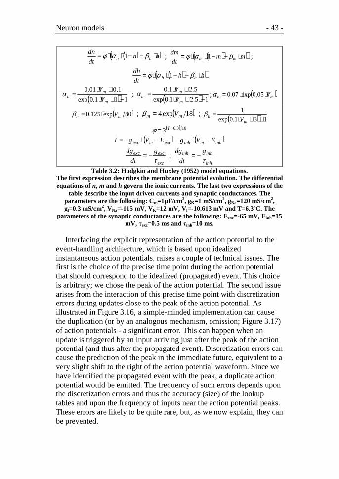
In order to further validate the simulation scheme, we have also compiled into tables the Hodgkin & Huxley model (1952) and evaluated the accuracy obtained with the proposed table-based methodology. Table 3.2 shows the differential expressions that define the neural model. We have also included expressions for synaptic conductances.
( ) ( ) ( )( ) mlmlNamNsKmKm CVVgVVhmgVVngI
dt
dV−−−⋅⋅⋅−−⋅⋅−= 34
Neuron models - 43 -
( )( )nndt
dnnn ⋅−−⋅⋅= βαφ 1 ; ( )( )mm
dt
dmmm ⋅−−⋅⋅= βαφ 1 ;
( )( )hhdt
dhhh ⋅−−⋅⋅= βαφ 1
( ) 111.0exp
1.001.0
−+⋅+⋅
=m
mn V
Vα ; ( ) 15.21.0exp
5.21.0
−+⋅+⋅
=m
mm V
Vα ; ( )mh V⋅⋅= 05.0exp07.0α
( )80exp125.0 mn V⋅=β ; ( )18exp4 mm V=β ; ( ) 131.0exp
1
++⋅=
mh V
β
( ) 103.63 −= Tφ ( ) ( )inhminhexcmexc EVgEVgI −⋅−−⋅−=
exc
excexc g
dt
dg
τ−= ;
inh
inhinh g
dt
dg
τ−=
Table 3.2: Hodgkin and Huxley (1952) model equations. The first expression describes the membrane potential evolution. The differential equations of n, m and h govern the ionic currents. The last two expressions of the
table describe the input driven currents and synaptic conductances. The parameters are the following: Cm=1µF/cm2, gK=1 mS/cm2, gNa=120 mS/cm2, gl=0.3 mS/cm2, VNa=-115 mV, VK=12 mV, Vl=-10.613 mV and T=6.3ºC. The
parameters of the synaptic conductances are the following: Eexc=-65 mV, Einh=15 mV, τexc=0.5 ms and τinh=10 ms.
Interfacing the explicit representation of the action potential to the event-handling architecture, which is based upon idealized instantaneous action potentials, raises a couple of technical issues. The first is the choice of the precise time point during the action potential that should correspond to the idealized (propagated) event. This choice is arbitrary; we chose the peak of the action potential. The second issue arises from the interaction of this precise time point with discretization errors during updates close to the peak of the action potential. As illustrated in Figure 3.16, a simple-minded implementation can cause the duplication (or by an analogous mechanism, omission; Figure 3.17) of action potentials - a significant error. This can happen when an update is triggered by an input arriving just after the peak of the action potential (and thus after the propagated event). Discretization errors can cause the prediction of the peak in the immediate future, equivalent to a very slight shift to the right of the action potential waveform. Since we have identified the propagated event with the peak, a duplicate action potential would be emitted. The frequency of such errors depends upon the discretization errors and thus the accuracy (size) of the lookup tables and upon the frequency of inputs near the action potential peaks. These errors are likely to be quite rare, but, as we now explain, they can be prevented.

Neuron models - 44 -
Figure 3.16: Output-spike duplication due to discretization errors. Discretization errors could allow an update shortly following an action
potential peak to predict the peak of the action potential in the immediate future, leading to the emission of an erroneous duplicate spike. (The errors have been
magnified for illustrative purposes.)

Neuron models - 45 -
Figure 3.17: Output-spike omission due to discretization errors. Discretization errors could allow an update shortly before an action potential
peak to set the membrane potential to a value slightly after the peak of the action potential, leading to the omission of a correct output spike.
We now describe one possible solution (which we have implemented) to this problem (see Figure 3.18). We define a "firing threshold" (θf; in practice -10mV). This is quite distinct from the physiological threshold, which is more negative. If the membrane potential exceeds θf, we consider that an action potential will be propagated under all conditions. We exploit this assumption by always predicting a propagated event if the membrane potential is greater than θf after the update, even if the "present" is after the action potential peak (in this case emission is immediate). This procedure ensures that no action potentials are omitted, leaving the problem of duplicates.
Neuron models - 46 -
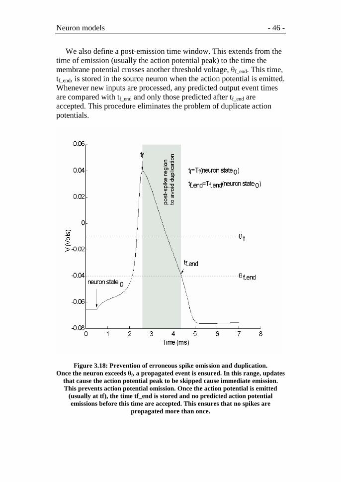
We also define a post-emission time window. This extends from the time of emission (usually the action potential peak) to the time the membrane potential crosses another threshold voltage, θf_end. This time, tf_end, is stored in the source neuron when the action potential is emitted. Whenever new inputs are processed, any predicted output event times are compared with tf_end and only those predicted after tf_end are accepted. This procedure eliminates the problem of duplicate action potentials.
Figure 3.18: Prevention of erroneous spike omission and duplication. Once the neuron exceeds θf, a propagated event is ensured. In this range, updates
that cause the action potential peak to be skipped cause immediate emission. This prevents action potential omission. Once the action potential is emitted
(usually at tf), the time tf_end is stored and no predicted action potential emissions before this time are accepted. This ensures that no spikes are
propagated more than once.

Neuron models - 47 -
In order to preserve the generality of this implementation, we chose to define these windows around the action potential peak by voltage level crossings. In this way the implementation will adapt automatically to changes of action potential waveform (possibly resulting from parameter changes). This choice entailed the construction of an additional large lookup table. Simpler implementations based upon fixed time windows could avoid this requirement. However, the cost of the extra table was easily borne.
We have compiled the model into the following tables:
- One table of seven dimensions for the membrane potential, Vm=f(∆t, gexc_0, ginh_0, n0, m0, h0, V0).
- Three tables of seven dimensions for the variables driving ionic currents, n=f(∆t, gexc_0, ginh_0, n0, m0, h0, V0), m=f(∆t, gexc_0, ginh_0, n0, m0, h0, V0), h=f(∆t, gexc_0, ginh_0, n0, m0, h0, V0).
- Two tables of two dimensions for the conductances, gexc=f(∆t, gexc_0), ginh=f(∆t, ginh_0).
- Two tables of 6 dimensions for the firing prediction , tf=f(gexc, ginh, n0, m0, h0, V0) and tf_end=f(gexc, ginh, n0, m0, h0, V0) . With θf=-0.01V and θf_end=-0.04V.
An accurate simulation of this model (as shown in Figure 3.19) requires approximately 6.15 Msamples (24.6 MB using 4-byte floating point data representation) for each seven-dimension table. We use a different number of samples for each dimension: ∆t(25), gexc_0(6), ginh_0(6), n0(8), m0(8), h0(8) and V0(14). The table calculation and compilation stage of this model requires approximately 4 minutes on a Pentium IV 1.8 Ghz.
3.4.1 Accuracy
Figure 3.19 shows an illustrative simulation of the Hodgkin and Huxley model using the table-based event-driven scheme. Note that the simulation engine is able to accurately jump from one marked instant (bottom plot) to the next one (according to either input or generated events). The membrane potential evolution shown in the bottom plot has been calculated using numerical method (continuous plot) and the

Neuron models - 48 -
marks (placed onto the continuous trace) have been calculated using the event-driven approach. We have also included the generated events using numerical calculation (vertical continuous lines) and those generated by the table-based event-driven approach (vertical dashed lines).
Figure 3.19: Event-driven simulation of an H&H model neuron. Note that in order to facilitate the comparison of the plots with the ones of other models, the variable (V) has been calculated using the following expression V=(-
Vm-Vrest)/1000 with Vrest=65 mV.
In order to evaluate the model accuracy we have adopted the same methodology described in the accuracy-and-speed section; we have simulated a single cell receiving an input spike train using numerical calculation to obtain a reference output spike train. Then, we have used the proposed table-based event-driven approach to generate another output spike train. The accuracy measurement is obtained calculating the van Rossum (2001) distance between the reference and the event-driven output spike trains. We have used a randomly generated test input spike train of average rate 300 Hz with a standard deviation of 0.7 and a uniform synaptic weight distribution in the interval [0.1,1] mS/cm2. Using the table sizes mentioned above, the van Rossum distance (with a time constant of 10 ms and the normalization mentioned in the accuracy-and-speed section) between the reference spike train and that obtained with the proposed method is 0.057 (in the same range as the Rossum distances obtained when comparing other simpler neural models, see Table 4.1). In fact, in order to obtain a
Simulation accuracy and speed - 49 -
similar accuracy using Euler numerical calculation a time step shorter than 65 µs is required.
4 Simulation accuracy and speed
To evaluate the performance of the implementation, in terms of accuracy and speed, and compare with other simulation methods, we have used the basic integrate-and-fire neuron model to make the corresponding measurements.
4.1 Simulation accuracy
An illustrative simulation is shown in Figure 4.1. A single cell with the characteristics of a cerebellar granule cell receives excitatory and inhibitory spikes (upper plots). We can see how the membrane conductances change abruptly due to the presynaptic spikes. The conductance tables emulate the excitatory AMPA-receptor-mediated and the inhibitory GABAergic synaptic inputs (the inhibitory inputs have a longer time constant). The conductance transients (excitatory and inhibitory) are also shown. The bottom plot shows a comparison between the event-driven simulation scheme, which updates the membrane potential at each input spike (these updates are marked with an x) and the results of an iterative numerical calculation (Euler method with a time step of 0.5 µs). This plot also includes the output spikes produced when the membrane potential reaches the firing threshold. The output spikes are not coincident with input events, although this is obscured by the time scale of the figure. It is important to note that the output spikes produced by the event-driven scheme are coincident with those of the Euler simulation (they superimpose in the bottom plot). Each time a neuron receives an input spike, both its membrane potential and the predicted firing time of the cell are updated. This only occurs very rarely, as the spacing of the events in the event-driven simulation illustrates.

Simulation accuracy and speed - 50 -
Figure 4.1: Single-neuron simulation. Excitatory and inhibitory spikes are indicated on the upper plots. Excitatory and
inhibitory conductance transients are plotted in the middle plots. The bottom plot is a comparison between the neural model simulated with iterative
numerical calculation (continuous trace) and the event-driven scheme, in which the membrane potential is only updated when an input spike is received (marked
with an "x").
It is difficult to estimate the appropriate size of the tables for a given accuracy. One of the goals of this simulation scheme is to be able to simulate accurately large populations of neurons, reproducing faithfully phenomena such as temporal coding and synchronization processes. Therefore, we are interested in reproducing the exact timing of the spikes emitted. In order to evaluate this, we need a way to quantify the difference between two spike trains. We used the van Rossum (2001) distance between two spike trains. This is related to the distance introduced by Victor and Purpura (1996; 1997), but is easier to calculate, with Eq. ( 4.1 ), and has a more natural physiological interpretation (van Rossum, 2001).
[ ]∫∞
−=0
22 )()(1
),( dttgtft
gfDc
tc Eq. ( 4.1 )
( ) ( ) ( )∑ −−−=M
i
ttti
ciettHtf / Eq. ( 4.2 )
In Eq. ( 4.2 ), H is the Heaviside step function (H(x)=0 if x<0 and H(x)=1 if x≥0) and M is the number of events in the spike train. In Eq. (

Simulation accuracy and speed - 51 -
4.1 ), the distance D is calculated as the integration of the difference between f and g, which are spike-driven functions with exponential terms, as indicated in Eq. ( 4.2 ). Note that the resulting distance and, indeed, its interpretation, depends upon the exponential decay constant, tc in Eq. ( 4.2 ), whose choice is arbitrary (van Rossum, 2001). We used tc = 10ms. The distance also depends upon the number of spikes in the trains. For this reason, we have chosen to report a crudely-normalised version D2(f,g)tc/M. Two trains differing only by the addition or removal of a single spike have a normalized distance of (1/2 M). Two trains differing only by the relative displacement of one spike by δt have a normalized distance of (1-exp(-|δt|/tc))/M.
In order to evaluate the accuracy of the EDLUT method and evaluate the influence of table size, we computed the neural model using iterative calculations and the EDLUT method and then calculated the distance between the output spike trains produced by the two methods.
Figure 4.2 illustrates how the accuracy of the event-driven approach depends on the synaptic weights of each spike, in an example using a Poisson input spike train. We plot as a function of synaptic weight the normalized van Rossum distance between the output spike trains calculated with the Euler method and obtained with EDLUT. Spikes with very low weights do not generate output events (either in the event-driven scheme or in the numerical computation one). Conversely, spikes with very large weights will always generate output events. Therefore, the deviation between the event-driven and the numerical approach will be low in both these cases. However, there is an interval of weights in which the errors are appreciable, because the membrane potential spends more time near threshold and small errors can cause the neuron to fire or not to fire erroneously. In general, however, a neuron will have a spread of synaptic weights and is unlikely to show such a pronounced error peak. Action potential variability in sub-threshold states is also seen in biological recordings (Stern et al, 1997), therefore a certain level of error may be affordable at a network scale.

Simulation accuracy and speed - 52 -
Figure 4.2: Simulation error depending on synaptic weights. The accuracy of the event-driven simulation depends on the weights of the
synapses, with maximal error (normalized van Rossum distance) occurring over a small interval of critical conductances. All synaptic weights were equal.
The accuracy of the event-driven scheme depends on the sampling resolution of the different axes in the tables. We varied the resolution of various parameters and quantified the normalized van Rossum distance of the spike trains produced, with respect to the 'correct' output train obtained from an iterative solution. The axes of the Vm and tf table were varied together, but the conductance lookup tables were not modified. Effective synaptic weights were drawn at random from an interval of [0.5, 2] nS, thus covering the critical interval illustrated in Figure 4.2. From Figure 4.3 we see that using a proposed initial table dimensions, the accuracy of ∆t and gexc are critical, but the accuracy of the event-driven scheme becomes more stable when table dimensions are above 1000 K samples. Therefore, we consider appropriate resolution values are the following: 16 values for gexc,t0 and ginh,t0, 64 values for ∆t and 64 values for Vm,t0. These dimensions will be used henceforth for this neuron model.

Simulation accuracy and speed - 53 -
Figure 4.3: Simulation error depending on table size. The accuracy of the event-driven approach depends on the resolution of the
different dimensions, and therefore on the table sizes. To evaluate the influence of table size on accuracy, we ran the simulations with different table sizes. For
this purpose, we chose an initial Vm table of 1000 K samples (64 values for ∆t, 16 values for gexc,t0, 16 values for ginh,t0 and 64 values for Vm,t0). We then halved the
size of individual dimensions, obtaining tables of size 500 K samples and 250 K samples from the original table of 1000 K samples. Finally, we doubled the
sampling density of individual dimensions to obtain the largest tables of 2000 K samples. For each accuracy estimation, we used an input train of 100 excitatory and 33 inhibitory spikes (which generates 26 output spikes when
simulated with iterative methods and high temporal resolution).

Simulation accuracy and speed - 54 -
Figure 4.4: Output spike trains for different table sizes. The first two plots represent the excitatory and inhibitory spikes. The E plots are the output events obtained with numerical iterative methods with different time
step resolutions (Euler method with 0.5 µs and with 2 µs). The other plots represent the outputs generated with the event-driven scheme using different table sizes: small (S) of 500 K elements, medium (M) of 1000 K elements and
large (L) of 2000 K elements. The subscripts indicate which dimension resolution has been doubled (or halved) from the Medium (M) size table.
Illustrative output spike trains for different table sizes, as well as the reference train, are shown in Figure 4.4. The spike trains obtained with the iterative method and the event-driven scheme are very similar for the large table with increased resolution in ∆t. A spurious spike difference is observed in the other simulations. Doubling the resolution in dimensions other than ∆t does not increase the accuracy significantly in this particular simulation. We can also see how the spike train obtained with the small tables is significantly different.
4.2 Simulation speed
With EDLUT, as described, the simulation time is essentially independent of the network size, depending principally on the rate of events that need to be processed. In other words, the simulation time depends on the network activity, as illustrated in Figure 4.5.

Simulation accuracy and speed - 55 -
Figure 4.5: Computation time. This figure represents the time taken to simulate 1 second of network activity on a Pentium IV (1.8 GHz) computer. Global activity represents the total number of
spikes per second in the network. The network size did not have a significant impact on the time required. The time was almost linear with respect to network
activity. The horizontal grid represents the real-time simulation limit, i.e. one second of simulation requiring one second of computation time.
The present implementation allows, for instance, the simulation of 8·104 neurons in real time with an average firing rate of 10 Hz on a 1.8 GHz Pentium IV platform. This implies the computation at a rate of 8·105 spikes/second as illustrated in Figure 4.5. Large numbers of synaptic connections of single neurons are efficiently managed by the two-stage strategy described in Figure 2.4. The size of the event queue is affordable, even in simulations with neurons with several thousands of synapses each.
The number of synapses that the simulation engine is able to handle is limited by memory resources. Each neuron requires 60 Bytes and each synapse 52 Bytes. Therefore, a simulation of 8·105 neurons consumes about 46 Mbytes and a total of 62·106 connections consumes about 3 Gbytes.

Simulation accuracy and speed - 56 -
In order to illustrate the potential of the EDLUT method we have compared the performance of this computation scheme with other methods (see Table 4.1). We have implemented three alternative strategies:
- Time-driven iterative algorithm with a fixed time step (TD-FTS). We have used the Runge-Kutta method with a fixed time step.
- Time-driven iterative algorithm with variable time step (TD-VTS). We use the Runge-Kutta method with step doubling and the Richardson extrapolation technique (Cartwright and Piro, 1992). In this case, the computational accuracy is controlled by defining the “error tolerance”. In this scheme, the iterative computations are done with time step sizes that depend on the smoothness of the function. If a calculation leads to an error estimation above the error tolerance the time step is reduced. On the other hand, if the error estimation is below this threshold the time step is doubled. This scheme is expected to be fast when only smooth changes occur in the neuronal states (between input spikes). Even though this method is time driven, its computation speed depends on the cell input in the sense that the simulation passes quickly through time intervals without input activity and when an input spike is received the computation approach reduces the time step to simulate accurately the transient behaviour of the cell. A similar simulation scheme with either global or independent variable time-step integration has been adopted in NEURON (Hines & Carnevale, 2001; Lytton and Hines, 2005).
- Pseudo-analytical approximation (PAA) method. In this case we have approximated the solution of the differential equations that govern the cell. In this way we can adopt an event-driven scheme similar to that proposed in Makino (2003) and Mattia & Del Giudice (2000), in which the neuron behaviour is described with analytical expressions. As in Makino (2003), the membrane potential is calculated with the analytical expression and the firing time is calculated using an iterative method based on Newton-Raphson. Since the differential equations defining the cell behaviour of our model have no analytical solution, we need to approximate a four-dimensional function. Even using advanced mathematical tools this represents a hard task. The accuracy of this approach depends significantly on how good this approximation is. In order to illustrate the complexity of the complete cell behaviour it is worth mentioning that the expression used was composed of 15 exponential functions.

Simulation accuracy and speed - 57 -
As shown in Table 4.1, even this complex approximation does not provide great accuracy, but we have nevertheless used it in order to estimate the computation time of this event-driven scheme.
- Event-driven based on Lookup tables (EDLUT). This is our approach, in which the transient response of the cell and the firing time of the predicted events are computed off-line and stored in lookup tables. During the simulations each neuronal state update is performed by taking the appropriate value from these supporting tables.
Normalized van Rossum
distance
Comput. time (s)
Time step (s)
56·10-5 0.061 0.286 43·10-5 0.033 0.363
Time driven with fixed time step
(TD-FTS) 34·10-5 0.017 0.462 Error
tolerance
68·10-5 0.061 0.209 18·10-5 0.032 0.275
Time driven with variable time step
(TD-VTS) 2·10-5 0.017 0.440
Pseudo analytical approximation method (PAA)
0.131 0.142
Table size (x106 samples)
1.05 0.061 0.0066 6.29 0.032 0.0074
Lookup-table-based event-driven scheme (EDLUT)
39.32 0.017 0.0085 Table 4.1: Performance evaluation of different methods.
Accuracy vs. computing time trade-off. We have focused on the computation of a single neuron with an input spike train composed of 100 seconds of excitatory
and inhibitory input spikes (average input rate 200 Hz) and 100 seconds of only excitatory input spikes (average input rate 10 Hz). Both spike trains had a standard deviation of 0.2 in the input rate and random weights (uniform
distribution) in the interval [0,0.8] nS for the excitatory inputs and [0,1] nS for the inhibitory inputs.
In order to determine the accuracy of the results, we obtained the “correct” output spike train using a time driven scheme with a very
Simulation accuracy and speed - 58 -
short time step. The accuracy of each method was then estimated by calculating the van Rossum distance (van Rossum, 2001) between the obtained result and “correct” spike train.
In all methods except the pseudo-analytical approach, the accuracy vs. computation time trade-off is managed with a single parameter (time step in TD-FTS, error tolerance in TD-VTS, and table size in EDLUT). We have chosen three values for these parameters that facilitate the comparison between different methods, i.e., values that lead to similar accuracy values. It is worth mentioning that all methods except the time-driven with fixed time step require a computation time that depends on the activity of the network.
Table 4.1 illustrates several points:
- The computing time using tables (EDLUT) of very different sizes is only slightly affected by the memory resource management units.
- The event-driven method based on analytical expressions is more than an order of magnitude slower than EDLUT (and has greater error). This is caused by the complexity of the analytical expression and the calculation of the firing time using the membrane potential expression and applying the Newton-Raphson method.
- The EDLUT method is about 50 times faster than the time-driven schemes (with an input average activity of 105 Hz).
4.3 Discussion and conclusions
A method for efficiently simulating large scale realistic neural networks has been implemented. Since most information transmission in these networks is accomplished by the so called action potentials, events which are considerably sparse and well-localized in time, it has been possible to dramatically reduce the computational load through the application of the event-driven simulation schemes.
Some complex neuronal models require the neural simulators to calculate large expressions, in order to update the neuronal state variables between these events. This requirement slows down these

Simulation accuracy and speed - 59 -
neural state updates, impeding the simulation of very active large neural populations in real-time. Moreover, neurons of some of these complex models produce firings (action potentials) some time after the arrival of the presynaptic potentials. The calculation of this delay involves the computation of expressions that sometimes are difficult to solve analytically. To deal with these problems, our simulation method makes use of precalculated lookup tables for both, fast update of the neural variables and the prediction of the firing delays, allowing efficient simulation of large populations with detailed neural models.
The proposed method efficiently splits the computational load into two different stages:
- Off-line neuronal model characterization. This preliminary stage requires a systematic numerical calculation of the cell model in different conditions, to scan its dynamics. The goal of this stage is to build up the neural characterization tables. This can be done by means of a large numerical calculation and the use of detailed neural simulators such as NEURON (Hines and Carnevale, 1997) or GENESIS (Bower and Beeman, 1998). In principle, this could even be done by compiling electrophysiological recordings (as described).
- On-line event-driven simulation. The computation of the simulation process jumps from one event to the next, updating the neuron states according to pre-calculated neuron characterization tables and efficiently managing newly produced events.
Mattia & Del Giudice (2000) used a cell model whose dynamics are defined by simple analytical expressions and Reutimann et al (2003) extended this approach by including stochastic dynamic. They avoided numerical methods by using a pre-calculated lookup tables. In this case, provided that the reordering event structure is kept of reasonable size (in those approaches large divergent connection trees may overload the spike reordering structure), the computation speed of these schemes is likely to be comparable to our approach, since the evaluation of a simple analytical expression and a lookup table consultation consume very little time.

Neural population synchronization - 60 -
5 Neural population synchronization
5.1 Introduction
There are many examples of electrical coupling between inhibitory neurons in the nervous system (Gibson et al, 1999; Long et al, 2004; Mann-Metzer and Yarom, 1999). Furthermore, electrical coupling has been proven to be an effective synchronization mechanism (Kopell et al, 2004; Kepler et al, 1990; Traub et al, 2000; Draghun et al, 1998).
Here we want to evaluate the simulation of electrical coupling within an event-driven scheme. For this purpose, we simulate a neural network of 100 cells receiving spikes at an average rate of 200 Hz with a standard deviation of 0.1 through excitatory synapses. These input spikes encode a constant bias and a random component. The cells are interconnected with inhibitory synapses and electrical coupling with an all-to-all topology. The network consists of 100 neurons with 100 input excitatory synapses (one per cell), 10000 inhibitory synapses and 10000 electrical connections. We have used neurons that intend to emulate cerebellar interneurons (Ros et al, 2005), using the following characterization parameters: membrane capacitance Cm=30 pF; time constants of the excitatory and inhibitory synapses τexc=0.5ms and τinh=2ms; resting conductance Grest=0.2 nS; excitatory and inhibitory reversal potentials Eexc=0 V and Einh=-80 mV; resting potential Erest= -70 mV; firing threshold Vth=-60 mV. This cell profile has been used to extract the characterization tables through intense numerical calculation using the SRM model (Gerstner et al, 2002) before the event driven simulation. The computing scheme processes everything in real-time (i.e. the computation time is much shorter than the simulated time; 1 second of simulation takes about 0.4 seconds). Since no numerical calculation is required during the event-driven simulation.
5.2 Results

Neural population synchronization - 61 -
In Figure 5.1 we show the obtained synchronization histograms using inhibition and electrical coupling. These results show the key phenomena obtained in detailed simulation (Kopell and Ermentrout, 2004) using a network of quadratic integrate-and-fire neurons (Latham et al, 2000); when using electrical coupling and inhibitory synapses, the synchronization was created quickly and multiple clusters of cells were not been observed (see Figure 5.1 C).
This validates our electrical coupling approach for this kind of simulations and proves event-driven simulation scheme to be an efficient tool to study this kind of processes or to apply them in neural network running in real time.

Neural population synchronization - 62 -
Figure 5.1: Neural-population synchronization histograms. A) Only electrical coupling of coefficient 0.02. B) Only inhibitory synapses Ginh=1.65nS. C) Inhibitory synapses (Ginh=1.65 nS) and electrical coupling
(coefficient of 0.02), there is no neuron firing asynchronously almost since the beginning. (The frequency is higher in A because there is no inhibition).

Cerebellum model simulation - 63 -
6 Cerebellum model simulation
6.1 Introduction
Although the cerebellum architecture has been studied for more than one hundred years (Ramón y Cajal et al., 1995; Golgi, 1967), its functional role is still an open topic. The cerebellum plays a major role in coordinated and accurate movements (Schweighofer et al., 1998a,b; Ito, 2001; Spoelstra et al., 2000; Arbib et al., 1995; Eskiizmirliler et al., 2002). It is thought to be an essential computing tissue for our daily manipulation tasks. Its regular topology has inspired many artificial neural network models in the past decades (Kettner et al., 1997; Schweighofer et al., 1998a; Medina et al., 1999) Furthermore, there are many research groups modelling in detail its cells (D'Angelo et al., 1995b; Bezzi et al., 2004; Steuber et al., 2004) in order to elucidate the specific computations that take place at each part of the cerebellum architecture.
In the robotic field there have been great advances (mainly in industrial applications). But most of the industrial robots use stiff joints and high-gain close-loop control. They are able to perform accurate trajectory-following adopting online close-loop error correction schemes. This strategy becomes possible due to the outstanding processing speed of current circuits that are able to calculate errors and deliver feedback correction signals on a millisecond time scale. On the other hand, biological systems suffer from delays in sensorimotor pathways up to several hundreds of milliseconds. This makes it impossible to apply online close-loop error correction strategies without having predictor modules able to abstract the kinematics and dynamic models of the platform. This becomes even more difficult because biological systems are based on joints with variable stiffness (agonist and antagonist muscle actuation) and low-gain control schemes. This is important because the dynamic model of the platform (for instance an arm-hand system) is likely to be significantly modified when manipulating objects of different weights. There are plenty of challenges in robotics such as the development of accurate low-gain control schemes for robotic platforms of several degrees of freedom (DOF) and non-stiff joints. The movement of stiff joints highly

Cerebellum model simulation - 64 -
facilitates control since it reduces (or even avoids) the necessity of dynamic models of the whole system. On the other hand, accurate control of stiff joints does not take advantage of the robot dynamics, wasting energy and therefore reducing the autonomy of the robot platform.
In this section, we try to emulate the learning strategy followed by biological systems to control low-gain, non-stiff robot platforms in the presence of sensorimotor pathways with delays of hundreds of milliseconds. More concretely, we study how a cerebellum model can abstract dynamics models of the robot platform in order to facilitate control by predicting and correcting errors in the motor space.
Fot this, we use a neural network modelling the cerebellum based on integrate-and-fire spiking neurons with conductance-based synapses. The neuron characteristics are derived from detailed models of the different cerebellar neurons.
The main plasticity in the cerebellar model is at the parallel fiber to Purkinje cell connections whose spike-time-dependent plasticity (STDP) is driven by the inferior olive (IO) activity, which encodes an error signal (using a novel probabilistic low-frequency model). We demonstrate the model for robot control in a target position reaching task. We evaluate the model performance relative to the dynamic model of the robot platform. Furthermore, we test how the system learns in a non-destructive way to reach different target positions (therefore abstracting a global dynamic model). To test the system's ability to self-adapt to different dynamical models, we present results in which the dynamics of the robotic platform changes significantly (friction and load carrying).
6.2 Cerebellar model
We simulated the cerebellum spiking neural model with EDLUT simulator (the event-driven simulator based on lookup tables described before; (Ros et al., 2006)) This software is particularly suited for a cerebellar model in which sparse activity is expected (Coenen et al., 2001; Schweighofer et al., 2001) in the numerous neurons of the granular layer (approximately 1011 granule cells (Kandel et al., 2000))

Cerebellum model simulation - 65 -
allowing real-time simulation of large-scale spiking neural networks. The EDLUT environment facilitates a direct interface to real robot platforms.
Lasting functional changes at a synaptic level can be driven by the coincidence of multiple signals at a single synaptic site (Brown et al., 1990). Long-term depression of the parallel fiber input to cerebellar Purkinje cells is a form of synaptic plasticity that can last from hours to days (Ito et al., 1982) and is thought to underlie several forms of associative motor learning (Mauk et al., 1998).
In the cerebellar model that we present, long-term depression (LTD) is induced by coincident activation of parallel fiber (PF) and climbing fiber (CF) synaptic inputs (see the learning-rules subsection below).
Previous modelling of cerebellar involvement in learning movement includes smooth pursuit eye movement learning of Kettner et al. (Kettner et al., 1997). In that work, the cerebellar nuclei cells were not implemented in the model, and analog units, not spiking neurons were used. Schweighofer et al. (Schweighofer et al., 1998a) proposed a model of the cerebellum focusing on the learning of the inverse dynamics of a two-link six-muscle arm model. Parallel fiber-Purkinje cell (PF-PC) LTD was biologically inspired, but long-term potention (LTP) was not and implemented as a weights normalisation process. Moreover, learning was performed over short trials only (less than 500 ms) and not continuously as in our contribution.
A few cerebellar models for eyelid conditioning have used spiking neurons (e.g. (Medina et al., 1999; HofstÄotter et al., 2002). Learning was based on spikes coincidences between neurons, but none used the same probabilistic low-frequency firing of the inferior olive in their learning rules.
We simulated the cerebellum spiking neural model (Boucheny et al., 2005; Arnold., 2001; Ros et al., 2006; Huang et al., 1998) with approximately 2100 units: 112 mossy fibers (MF), 2000 granule cells (GR) with their axons as parallel fibers (PF), 5 Golgi cells (GC), 32 inferior olive (IO) climbing fibers (CB), 32 purkinje cells (PC) and 16 deep cerebellar nuclei (DCN) cells.
Mossy fibers are implemented as leaky integrate-and-fire neurons. Their input current was determined by a radial basis function (RBF) of one of the sensory variables (target position or velocity) (Figure 6.1).

Cerebellum model simulation - 66 -
The RBF centers were evenly distributed across the sensory dimensions, and their variance were chosen to ensure small responses overlap from consecutive mossy fibers.
Figure 6.1: Encoding of mossy fibers. The analog to spikes transformation for driving the mossy fibers uses
overlapping radial basis functions (RBF). The example here makes reference to encoded joint variables (see Figure 6.9).
The inferior olive (IO) neurons synapse onto the Purkinje cells and contribute to direct the plasticity of PF-PC synapses. These neurons, however, fire at very low rates (less than 10 Hz), which appears problematic to capture the high-frequency information of the error signal of the task being learned. This apparent difficulty may be solved by their irregular firing (Kuroda et al., 2001; Schweighofer et al., 2004), which we exploit by statistically sampling the entire range of the error signal over multiple trials. This irregular firing was implemented using a Poisson model for spike generation.
Error correction is accomplished by changes in the activity of Purkinje cells that in turn influence the activity of the deep cerebellar nuclei cells (Purves et al., 2001), which afterwards is translated into analog torque correction signals for the robot.

Cerebellum model simulation - 67 -
6.3 Neuron models
To simulate the spiking neurons of this cerebellar model, we use the integrate-and-fire model with synaptic conductances described in the corresponding previous section. Modifying the neuron model parameter (Cm, τexc, τinh, grest, Eexc, Einh, Erest and Vth), different neuron types (granule cell, Purkinje cell and Golgi cell) have been characterized according to neurophysiological characterization studies (D'Angelo et al., 1995a,b; Maex et al., 1998; Barbour, 1993; Solinas et al., 2003). This neuron model is a modified version of the Spike-Response-Model (SRM) (Gerstner et al., 2002) widely used in the literature (Eckhorn et al., 1990; Schoenauer et al., 2002; Shaefer et al., 2002) to study, for example, temporal coding issues (Eckhorn et al., 2004).
In our model, the inferior olive cells transmit the error signal using probabilistic low-rate spikes. Mossy fibers carry sensorimotor signals encoded into rate coded spike trains (activity 0-100 Hz). And deep cerebellar nuclei cells provide spike trains which encode corrective motor torque signals.
6.4 Cerebellum model topology
The model reproduced the cerebellum's different functional and topological features (Andersen et al., 1992; Kandel et al., 2000): sparse coding at the parallel fibers (Coenen et al., 2001; Schweighofer et al., 2001), converging topology into Purkinje cells, Purkinje cell receiving a dedicated "teaching climbing fiber" from the inferior olive, inhibition to the granule cells from collector Golgi cells, etc. (see Table 6.1 and Figure 6.2)
Cell type Number Afferents from Efferents to
Granule 2000 4 mossy fibers 5 Golgi
32 Purkinje

Cerebellum model simulation - 68 -
Golgi 5 1000 granule 2000 granule
Purkinje 32 1500 granule
1 climbing fiber 4 DCN neurons
Table 6.1: Connectivity table of the cerebellar cells.
Figure 6.2: Cerebellum model diagram. Inputs about the movement (desired arm state and target information) are sent (upward arrow) to the two layers of mossy fibers (MF): distance to the target
and its absolute position in the experimental field (θtarg) and cartesian (dtarg) and coordinates and desired positions (θ) and speeds (‘θ) of the shoulder (s) and
elbow (e) joints along the trajectory. This information is conveyed to the two layers of granule cells (GR, 1000 neurons per layer), and to the deep cerebellar nuclei cells (DCN). Purkinje cells (PC), DCN and inferior olive neurons (IO) are
divided into 4 functional arrays, guided from the cerebellar microzones organisation, corresponding to the two commanded joints, in an agonist-
antagonist scheme. The 32 PC receive excitatory inputs from all the joints-related GR (ascending axons that maintain the cells in a state of excitability) and
from all parallel fibers PF with a probability pPC-PF = 0.8, and a learning connection from IO in a one-to-one scheme. In turn, the DCN receive two
inhibitory connections from PC of the same microzone. The teaching signal is processed by the IO cells (downward arrow top). The DCN firing rates are
interpreted as predictive positive (+) and negative (-) torque corrections (τ) for the shoulder (s) and (e) at the output of the cerebellum (downward arrow bottom). The numbers in brackets indicate the number of cells per layer.

Cerebellum model simulation - 69 -
6.5 Cerebellar Learning Rules
We have implemented learning at the parallel fibers to the Purkinje Cells connections (indicated by a ellipse in Figure 6.2) (Ito, 2001). The parallel fibers bring in the sensorimotor information and the Purkinje cells drive the cerebellum output through the deep-cerebellar-nuclei cells. The weight adaptation is driven by the activity generated by the inferior olive (IO), which encodes an error signal into a low frequency probabilistic spike train (from 0 to 10 Hz, average 1 Hz) (Kuroda et al., 2001; Schweighofer et al., 1998b).
We have modeled the inferior olive cell responses with a probabilistic Poisson process: given the error signal e(t) and a random number η(t) between 0 and 1, the cell fired a spike if e(t) > η (t), otherwise it remained silent (Boucheny et al., 2005). In this way, on one hand, a single spike reported accurately timed information regarding the instantaneous error; and on the other hand, the probabilistic spike sampling of the error ensured that the whole error region was accurately represented over trials with the cell firing at most 10 spikes per second. Hence, the error evolution is accurately sampled even at low frequency. The histogram of the inferior olive output spikes reproduces the error signal temporal trace; see Figure 6.3 for an example. This firing behavior is similar to the ones obtained in physiologial recordings (Kuroda et al., 2001).

Cerebellum model simulation - 70 -
Figure 6.3: Inferior-olive probabilistic encoding of the error. A) example of the error to be encoded. B) probabilistic firing of an inferior olive cell to the error in “A" (see text). C) mean firing rate of the cell averaged over all trials in “B". Notice that the maximum firing rate is close to 10 Hz. The smooth
curve shows the normalized input current to the cell related to the error amplitude. Notice how the cell never fires quite at the same moment relative to
the error, but encodes it nevertheless.
The long term potentiation (LTP) implemented at the parallel fiber to Purkinje cell synapses was a non-associative weight increase triggered by each granule cell spike (Eq. ( 6.1 )). The long term depression (LTD) was an associative weight decrease triggered by spikes from the inferior olive (Eq. ( 6.2 )). This model of LTD uses a temporal kernel (Figure 6.4), which correlates each spike from the inferior olive with the past activity of a granule cell (Lev-Ram et al., 2003) and shows a peak at 100 miliseconds (Kettner et al., 1997; Spoelstra et al., 2000; Raymond and Lisberger, 1998).

Cerebellum model simulation - 71 -
Figure 6.4: Spike Time Dependent Plasticity. Kernel used for granule cell (GR) and Purkinje cell (PC) synaptic long-term
depression, corresponding to the solution of a second order differential system. The kernel is convolved with the spike train of the afferent PF (all spikes emitted for t < 0). This provides a measure of past PF activity setting the eligibility of the
synapse to depression when the inferior olive (IO) neuron afferent to the PC emits a spike (t = 0).
LTP: )()( 00 tt GRαδω =∆ Eq. ( 6.1 )
LTD: ( ) ( )∫ ∞−−−=∆∀ IOt
GRIOii dttttKtw δ)(, 0 Eq. ( 6.2 )
The network maximizes learning (LTD) at synaptic sites in which the input parallel fiber delayed activity is highly correlated with the error signal from the inferior olive. Hence, this kernel produces a predictive corrective output in the network that helps the control task in the presence of significance transmission delays.
The teaching signal relies on the motor error, namely the discrepancy between the desired state of the joints at time t and the actual one. The error for each joint, respectively es and ee, is computed as the sum of the position and velocity errors, weighted by coefficients Kp = 10 and Kd = 23 (same for each joint). The signals are delayed in
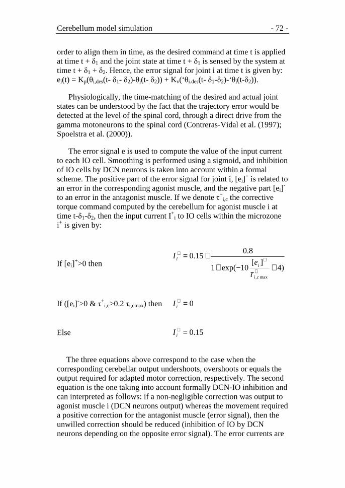
Cerebellum model simulation - 72 -
order to align them in time, as the desired command at time t is applied at time t + δ1 and the joint state at time t + δ1 is sensed by the system at time t + δ1 + δ2. Hence, the error signal for joint i at time t is given by: ei(t) = Kp(θi,des(t- δ1- δ2)-θi(t- δ2)) + Kv(‘θi.des(t- δ1-δ2)-‘θi(t-δ2)).
Physiologically, the time-matching of the desired and actual joint states can be understood by the fact that the trajectory error would be detected at the level of the spinal cord, through a direct drive from the gamma motoneurons to the spinal cord (Contreras-Vidal et al. (1997); Spoelstra et al. (2000)).
The error signal e is used to compute the value of the input current to each IO cell. Smoothing is performed using a sigmoid, and inhibition of IO cells by DCN neurons is taken into account within a formal scheme. The positive part of the error signal for joint i, [ei]
+ is related to an error in the corresponding agonist muscle, and the negative part [ei]
- to an error in the antagonist muscle. If we denote τ
+i,c the corrective
torque command computed by the cerebellum for agonist muscle i at time t-δ1-δ2, then the input current I+
i to IO cells within the microzone i+ is given by:
If [ei]+>0 then )4
][10exp(1
8.015.0
max,
+−++=
+
++
ci
ii e
I
τ
If ([ei]->0 & τ+i,c>0.2 τi,cmax) then 0=+
iI
Else 15.0=+iI
The three equations above correspond to the case when the corresponding cerebellar output undershoots, overshoots or equals the output required for adapted motor correction, respectively. The second equation is the one taking into account formally DCN-IO inhibition and can interpreted as follows: if a non-negligible correction was output to agonist muscle i (DCN neurons output) whereas the movement required a positive correction for the antagonist muscle (error signal), then the unwilled correction should be reduced (inhibition of IO by DCN neurons depending on the opposite error signal). The error currents are

Cerebellum model simulation - 73 -
normalized by esmax = 1000 and eemax = 600 for the shoulder and the elbow, respectively.
Figure 6.5: Input current to inferior olivary cells . Each olivary cell is related to the agonist muscle i and its firing is dependent on the error signal for this muscle (see text). This reflects the influence of the deep cerebellar nuclei feedback on the inferior olive together with an effector arm
system made of agonist and antagonist muscle pairs. The left side of the vertical line is for an error on the antagonist muscle, whereas the right side is for the
agonist muscle. The rule states that for an error on the antagonist muscle (left part), if the torque τ+
i,c > 0.2 τi,cmax, then the IO current I+i = 0 (bottom line),
otherwise I+i = 0.15 (top line).
6.6 Robot Platform
The robotic platform is a two-DOF arm (Figure 6.6 B). The two joints were not stiff (compliant) and the motors applied low forces. The platform allowed continuous measurements of the position of each joint. A pen or a weight could be attached to the arm's ending to change its dynamics.

Cerebellum model simulation - 74 -
Figure 6.6: Experimental robot platform. A) Representation of the arm in simulation. Each white point represents a target position (0-7) along a circle. B) Two degrees of freedom (DOF) robotic arm used
in the experiments. The motors have no gears and therefore are non-stiff low torque motors with nonlinearities difficult to control.
The control system was simulated on computer. To relieve the computer from interface computation and permit real-time communication with the robot, an FPGA-based board contained position acquisition modules and motor-driver controller circuits. The controller modules translated the motor-torque commands from the
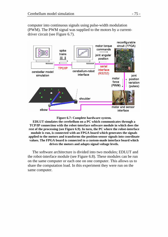
Cerebellum model simulation - 75 -
computer into continuous signals using pulse-width modulation (PWM). The PWM signal was supplied to the motors by a current-driver circuit (see Figure 6.7).
Figure 6.7: Complete hardware system. EDLUT simulates the cerebellum on a PC which communicates through a
TCP/IP connection with the robot-interface software module in which does the rest of the processing (see Figure 6.9). In turn, the PC where the robot-interface
module is run, is connected with an FPGA board which generates the signals applied to the motors and transforms the position-sensor signals into coordinate values. The FPGA board is connected to a custom-made interface board which
drives the motors and adapts signal voltage levels.
The software architecture is divided into two modules; EDLUT and the robot-interface module (see Figure 6.8). These modules can be run on the same computer or each one on one computer. This allows us to share the computation load. In this experiment they were run on the same computer.
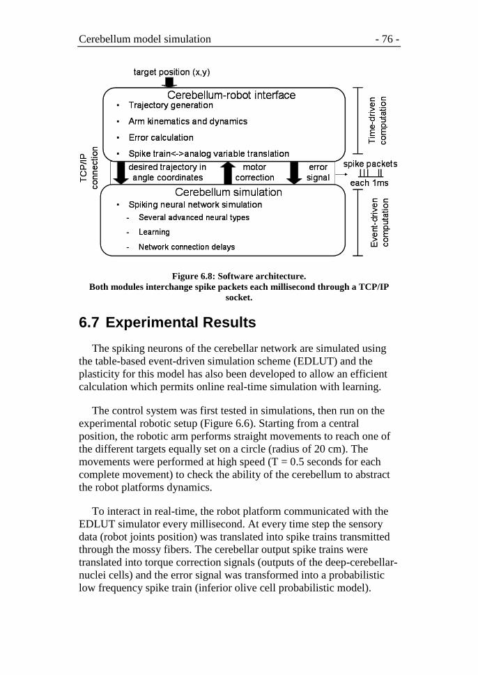
Cerebellum model simulation - 76 -
Figure 6.8: Software architecture. Both modules interchange spike packets each millisecond through a TCP/IP
socket.
6.7 Experimental Results
The spiking neurons of the cerebellar network are simulated using the table-based event-driven simulation scheme (EDLUT) and the plasticity for this model has also been developed to allow an efficient calculation which permits online real-time simulation with learning.
The control system was first tested in simulations, then run on the experimental robotic setup (Figure 6.6). Starting from a central position, the robotic arm performs straight movements to reach one of the different targets equally set on a circle (radius of 20 cm). The movements were performed at high speed (T = 0.5 seconds for each complete movement) to check the ability of the cerebellum to abstract the robot platforms dynamics.
To interact in real-time, the robot platform communicated with the EDLUT simulator every millisecond. At every time step the sensory data (robot joints position) was translated into spike trains transmitted through the mossy fibers. The cerebellar output spike trains were translated into torque correction signals (outputs of the deep-cerebellar-nuclei cells) and the error signal was transformed into a probabilistic low frequency spike train (inferior olive cell probabilistic model).
Cerebellum model simulation - 77 -
The simulations were run on a Pentium IV 2.8 GHz. There were 2100 neurons in the network for approximately 52 000 synaptic connections. During one second of simulation, the cerebellar network received an average of 395 spikes, delivered 405 output spikes, and processed 935 801 events. Under these conditions the simulator ran in real-time the full network and the input-output transformations.
Considering the duration of motor execution (T = 0.5 s) relative to the time delays in corticospinal loops (up to 300 ms), we made the assumption that each reaching movement was performed in open-loop (no high-level motor correction were applied while reaching the target). Corrective commands to compensate for dynamic perturbations were computed only by the cerebellar model.
A movement was separated in two phases:
- Open-loop movement phase: A movement lasted Tmove = 500 ms. The torque command applied to each articulation i was the sum of the cerebellar correction (τi,c) and the ith torque (τi), computed by a basic inverse dynamics model according to the desired kinematic trajectory (Figure 6.9). These two commands were sent to the limbs with a delay of δ1 = 50 ms.
- Post-movement phase: It was set to a duration of Tpost = 0.2 s. Its goal was to stop the movement of the arm, independently of its position relative to the target. The torque applied to each joint corresponds to the non delayed output of a derivative controller with a null-desired velocity: τi = Kvstopθi with Kvstop=10. The lack of delay in such a command in a human arm control model can be explained by a different motor strategy, consisting for example in a high level co-contraction command of the antagonist muscles controlling an articulation.
The architecture of the model for the generation of accurate fast arm reaching movements is illustrated in Figure 6.9. A minimum jerk model (Flash et al., 1985) was used to compute the desired smooth trajectory of the arm end-point towards the target at (OX, OY). The desired trajectory was expressed in Cartesian coordinates and transformed into joint coordinates by the inverse kinematics module. To solve the redundancy problem in the coordinates transformation, the robotic arm position was set to always be in a biological plausible posture, e.g that the angle between the two links of the limb were to remain positive.

Cerebellum model simulation - 78 -
Figure 6.9: Diagram of the arm-movement control system. The cerebellum acts as a predictive corrective module in the control loop. A
desired smooth trajectory toward the target was computed in Cartesian coordinates and transformed into joint coordinates. These desired arm states
were used at each time step to compute a crude torque command and to update the predictive corrective command of cerebellum. The cerebellum command
included information about the context of the movement. The two torques, crude and corrective torques, were summed to control the arm movement with a delay of δ1 = 50 ms. In turn, the error of the resulting trajectory was sensed at the level of the limb and sent back to the system with a delay of δ2 = 50 ms. This error was transformed to compute the cerebellum training signal by inferior olive neurons.
During the open-loop period of the movement, the torque commands sent to the joints were the sum of the output of a crude inverse dynamic controller and of the anticipative corrective cerebellar output. These torques were sent to the limb with a time delay δ1 = 50 ms.
The error in the execution of movement was computed at the level of the arm, and sent back to the system with a delay of δ2 = 50 ms. It was mainly used to determine the teaching signal conveyed by the inferior olive to the cerebellum to produce anticipative motor corrections. The error signal was composed of an angular position error and an angular velocity error for each articulation.
Finally, the cerebellar neural network received non delayed desired trajectory and movement context, and its output participated to the construction of the teaching signal with a delay of δ3 = 100 ms.

Cerebellum model simulation - 79 -
The inverse dynamics module was based on simplistic assumptions, such as mass homogeneity along the limbs and friction factor to compensate roughly for friction torques that reached 17 Ncm for the shoulder motor and 3 Ncm for the elbow. Other sources of dynamical perturbations, such as the forces exerted by the wires on the arm, were negligible compared to friction.
After defining an acceptable crude controller, we verified the repeatability of the movements and therefore of the errors of the crude controller. Indeed, the role of the cerebellum was to learn the anticipative corrections required across repeated trials of the same task. If the dynamics perturbations moving the arm to the desired paths varied too much across different trials under the same context (manipulating the same object) then no improvements could have been expected for the proposed control/correction scheme.
The model learned effectively and concurrently different target trajectories (Figure 6.10). An example shows the movement in x-y coordinates before and after learning (Figure 6.11). The cerebellum corrections build up over trials to compensate for the movement errors (Figure 6.12).

Cerebellum model simulation - 80 -

Cerebellum model simulation - 81 -
Figure 6.10: Target reaching experiments. A) Trajectory followed by the arm's ending. B) Average distance error computed over all trajectories when learning 1, 2, 3 or 4 different trajectories. C) Distance
error of the target No. 6 trajectory when learnt conjointly with 1,2, 3 or 4 different trajectories.
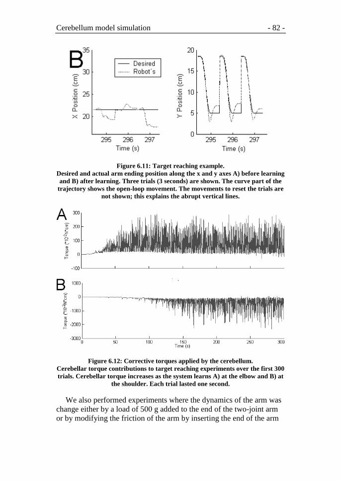
Cerebellum model simulation - 82 -
Figure 6.11: Target reaching example. Desired and actual arm ending position along the x and y axes A) before learning and B) after learning. Three trials (3 seconds) are shown. The curve part of the trajectory shows the open-loop movement. The movements to reset the trials are
not shown; this explains the abrupt vertical lines.
Figure 6.12: Corrective torques applied by the cerebellum. Cerebellar torque contributions to target reaching experiments over the first 300 trials. Cerebellar torque increases as the system learns A) at the elbow and B) at
the shoulder. Each trial lasted one second.
We also performed experiments where the dynamics of the arm was change either by a load of 500 g added to the end of the two-joint arm or by modifying the friction of the arm by inserting the end of the arm

Cerebellum model simulation - 83 -
into a sand pool (see Figure 6.13). The results of the cerebellum-driven improved trajectories are show in Figure 6.14.
Figure 6.13: Arm in the sand-pool context. The arm’s end is introduced into a sand pool to increase the friction during the movements. Note that since the arm’s end displaces the sand on the pool in each movement trial, the friction is modified between trials. This makes the learning
task more difficult.

Cerebellum model simulation - 84 -
Figure 6.14: Arm trayectory when learning in different contexts.
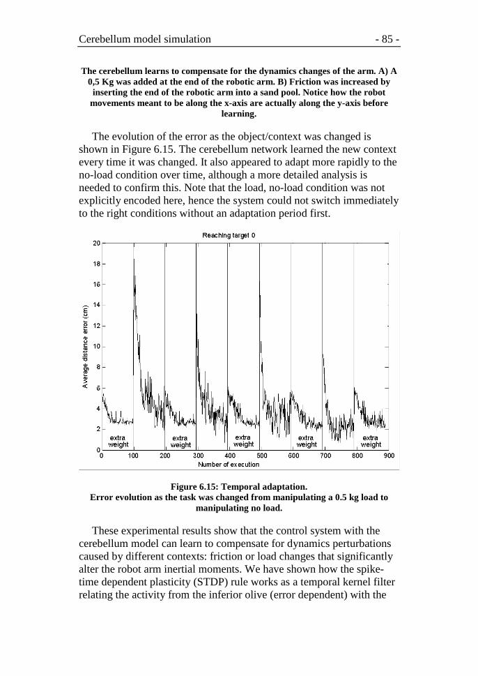
Cerebellum model simulation - 85 -
The cerebellum learns to compensate for the dynamics changes of the arm. A) A 0,5 Kg was added at the end of the robotic arm. B) Friction was increased by inserting the end of the robotic arm into a sand pool. Notice how the robot
movements meant to be along the x-axis are actually along the y-axis before learning.
The evolution of the error as the object/context was changed is shown in Figure 6.15. The cerebellum network learned the new context every time it was changed. It also appeared to adapt more rapidly to the no-load condition over time, although a more detailed analysis is needed to confirm this. Note that the load, no-load condition was not explicitly encoded here, hence the system could not switch immediately to the right conditions without an adaptation period first.
Figure 6.15: Temporal adaptation. Error evolution as the task was changed from manipulating a 0.5 kg load to
manipulating no load.
These experimental results show that the control system with the cerebellum model can learn to compensate for dynamics perturbations caused by different contexts: friction or load changes that significantly alter the robot arm inertial moments. We have shown how the spike-time dependent plasticity (STDP) rule works as a temporal kernel filter relating the activity from the inferior olive (error dependent) with the
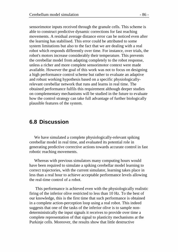
Cerebellum model simulation - 86 -
sensorimotor inputs received through the granule cells. This scheme is able to construct predictive dynamic corrections for fast reaching movements. A residual average distance error can be noticed even after the learning has stabilised. This error could be attributed to some system limitations but also to the fact that we are dealing with a real robot which responds differently over time. For instance, over trials, the robot's motors increase considerably their temperature. This prevents the cerebellar model from adapting completely to the robot response, unless a richer and more complete sensorimotor context were made available. However the goal of this work was not to focus on designing a high performance control scheme but rather to evaluate an adaptive and robust working hypothesis based on a specific physiologically-relevant cerebellar network that runs and learns in real time. The obtained performance fulfils this requirement although deeper studies on complementary mechanisms will be studied in the future to evaluate how the control strategy can take full advantage of further biologically plausible features of the system.
6.8 Discussion
We have simulated a complete physiologically-relevant spiking cerebellar model in real time, and evaluated its potential role in generating predictive corrective actions towards accurate control in fast robotic reaching movements.
Whereas with previous simulators many computing hours would have been required to simulate a spiking cerebellar model learning to correct trajectories, with the current simulator, learning takes place in less than a real hour to achieve acceptable performance levels allowing the real-time control of a robot.
This performance is achieved even with the physiologically realistic firing of the inferior olive restricted to less than 10 Hz. To the best of our knowledge, this is the first time that such performance is obtained in a complete action-perception loop using a real robot. This indeed suggests that one of the tasks of the inferior olive is to sample non-deterministically the input signals it receives to provide over time a complete representation of that signal to plasticity mechanisms at the Purkinje cells. Moreover, the results show that little destructive
Cerebellum model simulation - 87 -
interference occurred in learning the same task in different sensorimotor contexts, namely different overall target trajectories.
The robot arm we have used for the experiments has two non-stiff joints controlled with low torque motors. In order to accurately control this platform it is necessary to build a predictive dynamics model of the arm. The cerebellum network essentially fulfils this purpose.
Moreover, we implemented the delays in the sensorimotor pathways to evaluate the predictive strategy tested in this work. We implemented a STDP kernel filter that correlates the activity from the inferior olive (encoding the error using a probabilistic model) with the sensorimotor activity received through the parallel fibers. The correlation is done at the parallel fibers to Purkinje cells synaptic connections.
The experimental results show how the cerebellum-based system is able to adapt dynamically to different contexts. Future work will test sensorimotor encoding strategies to learn multiple models and context switching mechanisms to choose optimal control action with minimal delay and relearning.

Discussion and conclusions - 88 -
7 Discussion and conclusions
We have presented an event-driven network simulation scheme based on pre-calculated neural characterization tables. The use of such tables offers flexibility in the design of cell models while enabling rapid simulations of large-scale networks. The main limitation of the technique arises from the size of the tables for more complex neuronal models.
The aim of our method is to enable simulation of neural structures of reasonable size, based on cells whose characteristics cannot be described by simple analytical expressions. This is achieved by defining the neural dynamics using pre-calculated traces of their internal variables.
The proposed scheme represents a simulation tool that is intermediate between the very detailed simulators, such as NEURON (Hines and Carnevale, 1997) or GENESIS (Bower and Beeman, 1998), and the event-driven simulation schemes based on simple analytically-described cell dynamics (Delorme et al 1999, Delorme and Thorpe 2003). The proposed scheme is able to capture cell dynamics from detailed simulators and accelerate the simulation of large-scale neural structures. The approach as implemented here allows the simulation of 8•104 neurons with up to 6•107 connections in real time with an average firing rate of 10 Hz on a 1.8 GHz Pentium IV platform.
It is difficult to make a precise performance comparison between our method and previous event-driven methods, since they are based on different neuron models. Nevertheless, we have evaluated different computational strategies to illustrate the potential of our approach.
The method has been applied to simulations containing one-compartment cell models with exponential synaptic conductances (with different time constants) approximating excitatory AMPA receptor-mediated and GABAergic inhibitory synaptic inputs. The inclusion of new mechanisms, such as voltage-dependent channels is possible. However it would require the inclusion of new neural variables and thus new table dimensions. Although very complex models may eventually require lookup tables that exceed current memory capacities, we have shown how even a modest number of table dimensions can

Discussion and conclusions - 89 -
suffice to represent quite realistic neuronal models. We have also evaluated several strategies for compressing the tables in order to accommodate more complex models. Furthermore the proposed table-based methodology has been used to simulate the Hodgkin & Huxley model (1952).
The present event-driven scheme could be used for multi-compartment neuron models, although each compartment imposes a requirement for additional (one to three) dimensions in the largest lookup table. There are two ways in which multi-compartment neurons may be partially or approximately represented in this scheme. After preliminary studies, using suitable sampling schemes in order to achieve reasonable accuracy with a restricted table size, we can manage lookup tables of reasonable accuracy with more than seven dimensions. Therefore we can add two extra dimensions to enable two-compartment simulations. Quite rich cellular behaviour could be supplied by this extension. More concretely, we plan the addition of a second electrical compartment containing an inhibitory conductance. This new compartment will represent the soma of a neuron, while the original compartment (containing both excitatory and inhibitory conductances) will represent the dendrites. The somatic voltage and inhibitory conductance require two additional dimensions in the lookup table. With this model, it would be possible to separate somatic and dendritic processing, as occurs in hippocampal and cortical pyramidal cells, and implement the differential functions of somatic and dendritic inhibition (Pouille and Scanziani, 2001; Pouille and Scanziani, 2004) (note that most neurons do not receive excitation to the soma).
If individual dendrites can be active and have independent computational functions (this is currently an open question), it may be possible to approximate the dendrites and soma of a neuron as a kind of two-layer network (Poirazi et al, 2003), in which dendrites are actually represented in a manner similar to individual cells, with spikes that are routed to the soma (another cell) in the standard manner.
We have embedded spike-driven synaptic plasticity mechanisms in the event-driven simulation scheme. For this purpose, we have implemented learning rules approximated by exponential terms that can be computed recursively using an intermediate variable. Short-term dynamics (Mattia & Del Guidice, 2000) are also easy to include in the simulations. They are considered important in the support of internal

Discussion and conclusions - 90 -
stimulus representation (Amit, 1995; Amit & Brunel, 1997a; Amit & Brunel, 1997b) and learning.
Finally, we have used our method to simulate biologically-relevant neural networks. When simulating population synchronization, we have observed how the obtained results are equivalent to those used with more complex neural models and slower simulation methods. We have also simulated a complete spiking cerebellar model which effectively learns to improve the trajectory of a robotic arm in real time and different contexts.
In summary, we have implemented, optimized, and evaluated an event-driven network simulation scheme based upon prior characterization of all neuronal dynamics, allowing simulation of large networks to proceed extremely rapidly by replacing all function evaluations with table lookups. Although very complex neuronal models would require unreasonably large lookup tables, we have shown that careful optimization nevertheless permits quite rich cellular models to be used.

Publication of results - 91 -
8 Publication of results
Agís R., Carrillo R., Cañas A., del Pino B., Pelayo F.J., Entorno hardware/software para experimentación basado en micro robots, JCRA'2002: II Jornadas de computación reconfigurable y aplicaciones,Almuñecar (Granada) 18-20 Septiembre del 2002, 261-266 (ISBN: 84-699-9448-4)
Agis R., Ros E., Carrillo R., Ortigosa E.M., Pelayo F.J., Prieto A., Implementación en FPGAs de una Plataforma de Simulación de Neuronas de Pulsos, JCRA '2003: III Jornadas sobre Computación Reconfigurable y Aplicaciones, Configuración Reconfigurable FPGAs, pp.: 293-300, Madrid, 10-12 de septiembre de 2003 (ISBN: 84-600-9928-8)
Ortigosa E.M., Ortigosa P.M., Cañas A., Ros E., Carrillo R.R., Agis R., Implementación de Redes Neuronales con FPGAs para el Reconocimiento del Habla, JCRA '2003: III Jornadas sobre Computación Reconfigurable y Aplicaciones, Configuración Reconfigurable FPGAs, pp.: 301-308. Madrid, 10-12 de septiembre de 2003. (ISBN: 84-600-9928-8)
Eduardo Ros, Rodrigo Agís, Richard R. Carrillo, Eva M. Ortigosa, Francisco J. Pelayo, Alberto Prieto, Post-synaptic Time-dependent Conductances in Spiking Neurons: FPGA Implementation of a Flexible Cell Model, 7th International Work-Conference on Artificial and Natural Neural Networks, IWANN’2003: Lecture Notes in Computer Science, vol.: 2686, pp.: 145 – 152, Springer 2003. Maó, Menorca, Spain, June 3-6, 2003. (ISBN: 3-540-40211-X)
Eva M. Ortigosa, Antonio Cañas, Eduardo Ros, Richard R. Carrillo, FPGA implementation of a Perceptron-Like Neural Network for Embedded Applications, 7th International Work-Conference on Artificial and Natural Neural Networks, IWAN'2003, Lecture Notes in Computer Science, vol.: 2687, pp.: 1 – 8, Springer. Maó, Menorca, Spain, June 3-6, 2003. (ISBN: 3-540-40211-X)
Demo, From Visual Attention through to Motor Control, Mike Arnold, The Salk Institute for Biological Studies; Eduardo Ros, Rodrigo Agis, Richard Carrillo, Eva M. Orticosa University of Granada, Granada, Spain; Olivier Coenen, Sony Computer Science

Publication of results - 92 -
Laboratory, Paris; Fred Hamker, Westf. Wilhelms-Universität Münster, Germany; Chris Assad, Jet Propulsion Laboratory, California Institute of Technology, Pasadena; Marwan Jabri, Oregon Graduate Institute, Beaverton, Oregon; Terrence Sejnowski. NIPS: Neural Information Processing Systems, The Salk Institute for Biological Studies, La Jolla, USA, Tuesday, December 9-10, 2003.
O.J.M. Coenen, C. Boucheny, M. Bezzi, D. Marchal, M.P. Arnold, E. Ros, R. Carillo, E.M. Ortigosa, R. Agis, B. Barbour, A. Arleo, T. Nieus, E. D'Angelo, Adaptive spiking cerebellar models and real-time simulations, In: Society for Neuroscience Abstracts, No. 827.4, San Diego, USA. 2004
S. Mota, E. Ros, J. Díaz, E. M. Ortigosa, R. Agis, R. Carrillo, Real-time visual motion detection of overtaking cars for driving assistance using FPGAs. 14th International Conference, FPL '2004, pp. 1158-1161. Antwerp, Belgium, August 30-September 1, 2004. (ISBN: 3-540-22989-2)
Javier Díaz, Eduardo Ros, Sonia Mota, Richard Carrillo, Rodrigo Agis, Real time optical flow processing system, 14th International Conference,FPL '2204, pp 617-626. Antwerp, Belgium, August 30-September, 2004. (ISBN: 3-540-22989-2)
Agís R, Ros E, Díaz J, Mota S, Carrillo R, Ortigosa E, Pelayo F, Prieto A. Sistema de control basado en visión y propiacepción de robots con FPGA, JCRA'2004: IV Jornadas sobre Computación Reconfigurable y Aplicaciones, Configuración Reconfigurable FPGAs, pp. 667-674. Barcelona 13-15 de Septiembre, 2004 (ISBN: 84-688-7667-4)
Javier Díaz, Eduardo Ros, Sonia Mota, Eva M. Orticosa, Richard Carrillo, Rodrigo Agis, Cómputo de flujo óptico en tiempo real mediante FPGAs. JCRA'2004: IV Jornadas sobre Computación Reconfigurable y Aplicaciones, Configuración Reconfigurable FPGAs pp. 481-488, Barcelona 13-15 de Septiembre, 2004. (ISBN: 84-688-7667-4).
Antonio Martinez, Francisco Pelayo, Christian A. Morillas, Samuel Romero, Richard R. Carrillo, Begoña del Pino, Generador automático de sistemas bioinspirados de visión en hardware reconfigurable, JCRA '2004: IV Jornadas sobre Computación Reconfigurable y Aplicaciones, Configuración Reconfigurable FPGAs. pp 597-603. Barcelona 13-15 de Septiembre, 2004. (ISBN: 84-688-7667-4).

Publication of results - 93 -
R. Agis, R. Carrillo, V. Moran, A.Gonzalez, C. Morillas, F. Pelayo and J.L.Bernier, Monitoring a mobile robot using a web interface, III International conference on Multimedia and ICTs in Education (mICTE2005), pp. 1288-1293, Vol III. Caceres June 7-10th 2005. (ISBN: 84-609-5994-5)
R. Carrillo, Eduardo Ros, Eva M Ortigosa, Boris Barbour and Rodrigo Agis. Lookup Table Powered Neural Event-Driven Simulator, 8th Internacional Work Conference on Artificial Neural Networks, IWANN 2005, pp 168-175, Vilanova I la Geltrú, Barcelona, Spain, June 8-10, 2005. (ISBN-13: 978-3-540-26208-4)
Eduardo Ros, Eva M. Ortigosa, Rodrigo Agis, Richard Carrillo, Alberto Prieto and Mike Arnold. Spiking Neurons Computing Platform. 8th Internacional Work Conference on Artificial Neural Networks, IWANN 2005, pp 168-175. Vilanova I la Geltrú, Barcelona, Spain, June 8-10, 2005. (ISBN-13: 978-3-540-26208-4)
C. Boucheny, R. Carrillo, E. Ros, O. J.-M. Coenen, Real-Time Spiking Neural Network: An Adaptive Cerebellar Model. 8th Internacional Work Conference on Artificial Neural Networks, IWANN 2005, pp 136-144. Vilanova I la Geltrú, Barcelona, Spain, June 8-10, 2005. (ISBN-13: 978-3-540-26208-4)
Eduardo Ros, Richard R. Carrillo, Boris Barbour, Christian Boucheny, Olivier Coenen. Event-driven simulation of neural population synchronization facilizated by electrical coupling. IPCAT'2005: Sixth International Workshop on Information Processing in Cell and Tissues. pp 290-303, York, UK. August 30-September 1, 2005
Rodrigo Agis, Eduardo Ros, F.J.Pelayo, Richard Carrillo, Eva Ortigosa, Rafael Rodríguez, Javier Díaz, Sonia Mota. Sistema evolutivo de control de un brazo: Optimización de constantes dinámicas. Dentro del congreso español de informática (CEDI 2005), Jornadas sobre Computación Reconfigurable y Aplicaciones (JCRA 2005), pp 311-316, Granada 13-16 Septiembre, España, (ISBN:84-9732-439-0)
Eduardo Ros, Eva M. Ortigosa, Rodrigo Agís, Richard Carrillo and Mike Arnold. Real-time computing platform for spiking neurons (RT-Spike). IEEE Transactions on Neural Networks. Vol 17. p 1050-1063. July/2006
Rodrigo Agís, Javier Díaz, Eduardo Ros, Richard Carrillo, Eva. M. Ortigosa, Event-driven simulation engine for spiking neural networks on a chip, International workshop on applied

Publication of results - 94 -
reconfigurable computing (ARC2006) delft, the Netherlands, march 1-3, 2006. (Lecture Notes in Computer Science) Vol 3985. 36-45.
R. Agís, J. Díaz, E. Ros, R. Carrillo, E. M. Ortigosa, Hardware Event-driven Simulation Engine for Spiking Neural Networks, International Journal of Electronics (Taylor & Francis Group), 2006, (ISSN (Print): 0020-7217, ISSN (Online): 1362-3060) S.C.I. (2005): 0.213
J. Díaz, E. Ros, R. Carrillo y A. Prieto, Real-time system for high-image-resolution disparity, IEEE Trans. on Image Processing, 2006, (ISSN: 1057-7149), (S.C.I. (2005): 2.428)
Ros, E. Carrillo, R, Ortigosa, E. M., Barbour, B, Agís, R., Event-Driven Simulation Scheme for Spiking Neural Networks Using Lookup Tables to Characterize Neuronal Dynamics, Neural Comput. 2006 18: 2959-2993.
R.R. Carrillo, E. Ros, S. Tolu, T. Nieus, E. D'Angelo, Event-driven simulation of cerebellar granule cells, 7th International workshop on information processing in cell and tissues (IPCAT'2007), 29th-31st August 2007, Oxford, UK
R.R. Carrillo, E. Ros, C. Boucheny, O. J-M D Coenen, A cerebellum-like spiking neural network for robot control, 7th International workshop on information processing in cell and tissues (IPCAT'2007), 29th-31st August 2007, Oxford, UK

Bibliography - 95 -
Bibliography
Aho, A. V. Hopcroft, J. E. and Ullman, J. D. (1974). The design and analysis of computer algorithms. Reading, MA, Addison-Wesley.
Albus, J.S., 1971. A theory of cerebellar function, Math. Biosci 10, 25-61.
Amit, D. J. (1995). The Hebbian paradigm reintegrated: Local reverberations as internal representations. Behavioural and Brain Sciences, 18, 617-657.
Amit, D.J. and Brunel, N. (1997a). Model of global spontaneous activity and local structured (learned) delay activity during delay periods in cerebral cortex. Cerebral Cortex, 7, 237-252.
Amit, D.J. and Brunel, N. (1997b). Dynamics of a recurrent network of spiking neurons before and following learning. Network, 8, 373-404.
Andersen, B. B., Korbo, L., Pakkenberg, B., A quantitative study of the human cerebellum with unbiased stereological techniques. The Journal of comparative Neurology, Vol 326 (4), 1992, pp: 549-560.
Arbib, M.A. Schweighofer, N.,, Thach, W.T., Modeling the cerebellum: from adaptation to coordination. Motor Control and Sensory-Motor Integration: Issue and Directions, D.J. Glencross and J.P. Piek. Eds. Amsterdam, Elsevier, (1995) 1136.
Armano, S., Rossi, P., Taglietti, V., D'Angelo, E., 2000. Long-term potentiation of intrinsic excitability at the mossy fiber granule cell synapse of rat cerebellum. J Neurosci 15, 5208-5216.
Arnold, M., Feedback learning in the olivarycerebellar system, PhD Thesis, The University of Sydney, 2001.
Barbour, B. Synaptic currents evoked in Purkinje cells by stimulating individual granule cells. Neuron 11: 759-769, 1993
Bezzi, M., Nieus, T., Arleo, A., D'Angelo, E., Coenen O. J.-M. D., 2004. Information transfer at the mossy fiber granule cell synapse of the cerebellum. 34th Annual Meeting, Society for Neuroscience, San Diego, CA, USA.
Bezzi, M., Nieus, T., Arleo, A., D'Errico, A., D'Angelo E., Coenen, O. J. -M. D., 2006. Quantitative characterization of information

Bibliography - 96 -
transmission in a single neuron. The EPFL-Latsis Symposium Dynamical principles for neuroscience and intelligent biomimetic devices, Lausanne.
Bezzi, M., Nieus, T., Coenen, O. J-M, D'Angelo, E., 2004. An integrate-and-fire model of a cerebellar granule cell. Neurocomputing 58-60, 593-598.
Bi, G., and Poo, M. (1998). Synaptic modifications in cultured hippocampal neurons: dependence on spike timing, synaptic strength, and postsynaptic cell type. J. Neurosci. 18, 10464-10472.
Boucheny, C., Carrillo, R., Ros, E., Coenen, O. J-M D. (2005). Real-Time spiking neural network : an adaptive cerebellar model, Lecture Notes in Computer Science. 3512, 136-144.
Bower, J.M. and Beeman, B. (1998). The book of GENESIS. New York. Springer Verlag.
Braitenberg, V. & Atwood R.P. (1958). Morphological observations on the cerebellar cortex. J. Comp. Neurol. 109.1-33.
Brown, T. H., Kairiss, E. W., Keenan, C. L. Hebbian synapses: biophysical mechanisms and algorithms. Annu. Rev. Neurosci. 13, 1990, 475-511.
Brunel, N. and Hakim, V. (1999). Fast global oscillations in networks of integrate-and-fire neurons with low firing rates. Neural Computation, 11. 1621-1671
Cartwright, J.H.E. and Piro, O. (1992). The dynamics of Runge-Kutta methods, Int. J. Bifurcation and Chaos 2, 427-449.
Chez, C., 1991. The Cerebellum. In Principles of Neural Science (Third Edition), Edited by Kandel, E., Schwartz, J.H. and Jessel. 626-645.
Chowdhury R.A. and Kaykobad M. (2001). Sorting using heap structure. Proceedings of Int. Conf. on Comp. and Inf. Tech. Dhaka, Bangladesh, 26-30.
Coenen, O. J.-M. D., Arnold, M. P., Sejnowski, T.J., Jabri, M.A., 2001. Parallel fiber coding in the cerebellum for life-long learning. Autonomous Robots 11(3), 291-297.
Coenen, O., Bezzi, M., Arleo, A., Nieus, T., D'Errico, A., D'Angelo, E., 2007. Information theoretic quantification of neural transmission following changes in release probability. Computational and Systems Neuroscience (COSYNE 07), Salk Lake City, UTAH.

Bibliography - 97 -
Conn, A.R., Gould, N.I.M. and Toint, P.L. (2000). Trust-Region Methods. SIAM.
Contreras-Vidal, J. L., Grossberg, S., Bullock, D., 1997. A neural model of cerebellar learning for arm movement control: cortico-spino-cerebellar dynamics. Learning and memory 3(6), 475-502.
Cormen, T. H., Lierson, C. E. and Rivest, R. L. (1990). Introduction to algorithms. MIT Cambridge press, 140-152.
D’Angelo, E., Nieus, T., Maffei, A., Armano, S., Rossi, P., Taglietti, V., Fontana, A., Naldi, G., 2001. Theta-frequency bursting and resonance in cerebellar granule cells: Experimental Evidence and Modelling of a slow K+-dependent mechanism. The Journal of Neuroscience, 21(3), 759-770.
D'Angelo, E., De Filippi, G., Rossi, P., Taglietti, V., Synaptic excitation of individual rat cerebellar granule cells in situ: evidence for the role of NMDA receptors. J. Physiol. (Lond.) 482: 397413, 1995.
D'Angelo, E., Nieus, T., Bezzi, M., Arleo, A., Coenen, O. J.M.D., 2005. Modeling Synaptic Transmission and Quantifying Information Transfer in the Granular Layer of the Cerebellum. Lecture Notes in Computer Science 3512, 107-114.
Delorme, A., Gautrais, J. van Rullen, R., Thorpe, S. (1999). SpikeNET: A simulator for modelling large networks of integrate and fire neurons. In J. M. Bower (Ed.), Computational Neuroscience: Trends in research 1999, Neurocomputing, Vols. 26-27, 989-996.
Delorme, A., Thorpe, S. (2003). SpikeNET: An event-driven simulation package for modelling large networks of spiking neurons. Network: Computation in Neural Systems,14, 613-627.
Eckhorn, R., Gail, A. M., Bruns, A., Gabriel, A., Al-Shaikhli, B., Saam, M., Different types of signal coupling in the visual cortex related to neural mechanisms of associative processing and perception, IEEE Transactions on Neural Networks, vol. 15(5), 2004, 1039-1052.
Eckhorn, R.; Bauer, R.; Jordan, W.; Brosh, M.; Kruse, W.; Munk, M.; Reitböck, (1988). Coherent oscillations: A mechanism of feature linking in the visual cortex? Biol. Cyber. 60, 121-130.
Eckhorn, R.; Reitböck, H.J.; Arndt, M.; Dicke, D. (1990). Feature Linking via Synchronization among Distributed Assemblies: Simulations of Results from Cat Visual Cortex. Neural Computation, 2, 293-307.

Bibliography - 98 -
Eskiizmirliler, S., Forestier, N., Tondu, B., Darlot, C., A model of the cerebellar pathways applied to the control of a single-joint robot arm actuated by McKibben artificial muscles. Biological Cybernetics, 86, 2002 379-394.
Flash, T., Hogans, N., The Coordination of Arm Movements: An Experimentally Confirmed Mathematical Model. The Journal of Neuroscience Vol. 5, No 7. July, 1985, pp. 1688-1703.
Forti, L., Cesana, E., Mapelli, J., D'Angelo, E., 2006. Ionic echanisms of autorhythmic firing in rat cerebellar Golgi cells. Journal of Physiology 574(3), 711-729.
Gerstner, W., & Kistler, W. (2002). Spiking neuron models: Single neurons, populations, plasticity. Cambridge: Cambridge University.
Gibson, J. R., Beierlein, M., Connors, B. W., 1999. Two electrically coupled inhibitory networks. Nature 402(4), 75-79.
Golgi C., The neuron doctrine: theory and facts. In: Nobel Lectures: Physiology or Medicine, [1906], 1967, 1901-1921, 189-217. Amsterdam: Elsevier.
Graβmann, C., Anlauf, J. K.: Fast digital simulation of spiking neural networks and neuromorphic integration with SPIKELAB. International Journal of Neural Systems, 9(5). (1999) 473-478
Hebb, D.O. (1949). The organization of behaviour. Wiley, New York.
Hines, M.L. and Carnevale, N.T. (1997). The NEURON simulation environment. Neural Computation, 9, 1179-1209.
Hodgkin, A.L. & Huxley, A.F. (1952). A quantitative description of membrane current and its application to conduction and excitation in nerve. Journal of Physiology, 117, 500-544.
Hofstötter, C., Mintz, M., Verschure, P. F. M. J., Oct. 2002. The cerebellum in action: a simulation and robotics study. European Journal of Neuroscience 16 (7), 1361-1376.
Horn, R. and Marty, A. (1988). Muscarinic activation of ionic currents measured by a new whole-cell recording method. Journal of General. Physiology. 92, 145-159.
Huang, J., Jabri, M. A., Coenen, O. J.-M. D., October 1998. Models of basal ganglia and cerebellum for sensorimotor integration and predictive control in real-time robot navigation, Laboratory Report, Sydney University.

Bibliography - 99 -
Ito, M., Cerebellar long-term depression: characterization, signal transduction, and functional roles. Physiological Reviews 81(3), 2001, 1143-1195.
Ito, M., Kano, M. Long-lasting depression of parallel fiber-Purkinje cell transmission induced by conjunctive stimulation of parallel fibers and climbing fibers in the cerebellar cortex. Neurosci. Lett. 33, 1982, 253-258.
Izhikevich, E. M., 2001. Resonate-and-fire neurons. Neural Networks 14, 883-894.
Kandel, E. R., Schwartz, J. H., Jessell, T. M., 2000. Principles of Neural Science. McGraw-Hill Professional Publishing, New York.
Karlton, P.L., Fuller, S.H., Scroggs, R.E., Kaehler, E.B. (1976). Performance of height-balanced trees. In Information retrieval and language processing. Communications of ACM. 19 (1), 23-28.
Kepler, T.B., Marder, E., and Abbott, L.F., 1990. The effect of electrical coupling on the frequency of model neuronal oscillators. Science, 248, 83-85.
Kettner, R.E., Mahamud, S., Leung, H., Sittkoff, N., Houk, J.C., Peterson, B.W., Barto, A.G.,Prediction of complex two-dimensional trajectories by a cerebellar model of smooth pursuit eye movement. Journal of Neurophysiology 77(4), 1997, 2115-2130.
Koch, C., 1999. Biophysics of computation: information processing in single neurons. New York, NY: Oxford University Press.
Kopell, N. and Ermentrout, B., 2004. Chemical and electrical synapses perform complementary roles in the synchronization of interneuronal networks. Proceedings of the National Academy of Sciences of the United States of America. 101(43), 15482-15487.
Kuroda, S., Yamamoto, K., Miyamoto, H., Doya, K., Kawato, M., Statistical characteristics of climbing fiber spikes necessary for efficient cerebellar learning. Biol. Cybern., 84, (3), 2001, 183-192.
Latham, P. E., Richmond , B.J., Nelson, P. G., Nirenberg, S. ,2000. Intrinsic dynamics in neuronal networks. I. Theory. J. Neurophysiol. 83(2), 808-827.
Lev-Ram, V., Mehta, S.B., Kleinfeld, D., Tsien, R.Y., Reversing cerebellar long-term depression., Proceedings of the National Academy of Sciences 100(26), 2003, 15989-15993.

Bibliography - 100 -
Long M.A., Landisman C.E., Connors B.W., 2004. Small clusters of electrically coupled neurons generate rhythmic in the thalamic reticular nucleus. Journal of Neuroscience. 24(2),341-349.
Lytton, W.W. and Hines, M.L. (2005). Independent Variable Time-Step Integration of Individual Neurons for Network Simulations. Neural Computation, 17, 903-921.
Maex, R., De Schutter, E., Synchronization of Golgi and Granule Cell Firing in a Detailed Network Model of the Cerebellar Granule Cell Layer. The Journal of Neurophysiology Vol. 80 No. 5 November, 1998, 2521-2537.
Magistretti, J., Castelli, L., D'Angelo, E., 2006. Kinetic and functional analysis of transient, persistent, and resurgent sodium currents in rat cerebellar granule cells in situ. Journal of Physiology 573, 83-106.
Makino, T. (2003). A Discrete-Event Neural Network Simulator for General Neuron Models. Neural Computing and Applications, 11, 210-223.
Mann-Metzer, P. and Yarom, Y., 1999. Electrotonic Coupling Interacts with intrinsic properties to generate synchronized activity in cerebellar networks of inhibitory interneurons. The Journal of Neuroscience. 19(9), 3298-3306.
Mapelli, J., D'Angelo E., 2007. Synaptic inhibition determines the spatial organization of long-term synaptic plasticity at the input stage of the cerebellum. Journal of Neuroscience 27(6), 1285-1296.
Marr, D., 1969. A theory of the cerebellar cortex. Journal of Physiology 202, 437-470.
Mattia, M., & Del Giudice, P. (2000). Efficient event-driven simulation of large networks of spiking neurons and dynamical synapses. Neural Computation, 12(10), 2305-2329.
Mauk, M. D., Garcia, K. S., Medina, J. F., Steele, P. M., Does cerebellar LTD mediate motor learning? Toward a resolution without a smoking gun. Neuron 20, 1998, 359-362.
Medina, J.F., Mauk, M.D., Simulations of cerebellar motor learning: computational analysis of plasticity at the mossy fiber to deep nucleus synapse. The Journal of Neuroscience 19(16), 1999), 71407151.
Mitchell, S.J., Silver, R.A. (2003). Shunting inhibition modulates neuronal gain during synaptic excitation. Neuron, 38, 433–445.

Bibliography - 101 -
Neyton, J., and Trautmann, A.. 1985. Single-channel currents of an intercellular junction. Nature, 317, 331-335.
Nieus, T., Sola, E., Mapelli, J., Saftenku, E., Rossi, P., D'Angelo, E., 2006. Regulation of repetitive neurotransmission and firing by release probability at the input stage of cerebellum: experimental observations and theoretical predictions on the role of LTP. Journal of Neurophysiology 95, 686-699.
Nusser, Z., Cull-Candy, S., Farrant, M. (1997). Differences in synaptic GABA(A) receptor number underlie variation in GABA mini amplitude. Neuron, 19(3):697-709.
Philipona, D., Coenen, O. J.-M. D., 2004. Model of granular layer encoding of the cerebellum. Neurocomputing 58-60, 575-580
Poirazi, P., Brannon, T., Mel, B.W. (2003). Pyramidal neuron as two-layer neural network. Neuron. 37(6), 989-999.
Pouille, F., Scanziani, M. (2001). Enforcement of temporal fidelity in pyramidal cells by somatic feed-forward inhibition. Science, 293(5532), 1159-1163.
Pouille, F., Scanziani, M. (2004). Routing of spike series by dynamic circuits in the hippocampus. Nature, 429(6993), 717-723.
Prinz, A.A., Abbott, L.F., Marder, E. (2004). The dynamic clamp comes of age. Trends Neurosci. 27, 218-24.
Pugh, W. (1990). Skip lists: A probabilistic alternative to balanced trees. Communications of the ACM, 33(6), 668–676.
Purves, D., Augustine, G. J., Fitzpatrick, D., Katz, L. C., Lamantia, A., McNamara, J. O., Williams, S. M., Neuroscience (Second Edition), Sinauer Associates, Inc., 2001.
Ramón y Cajal, S., Histology of the Nervous System of Man and Vertebrates. N Swanson, LWSwanson (transl). Vols. 1, 2. New York: Oxford Univ. Press. [1909], 1995.
Raymond, J. L., Lisberger, S. G., Nov 1 1998. Neural learning rules for the vestibulo-ocular reflex. Journal of Neuroscience 18 (21), 9112-9129.
Reutimann, J., Giugliano, M., Fusi, S. (2003). Event-driven simulation of spiking neurons with stochastic dynamics. Neural Computation, 15, 811-830.

Bibliography - 102 -
Richardson, M., Brunel, N., Hakim, V., From subthreshold to firing-rate resonance. Journal of Neurophysiology 89, 2538-2554.
Ros, E., Carrillo, R. R., Ortigosa, E. M., Barbour, B., Ags. R., 2006. Event-Driven Simulation Scheme for Spiking Neural Networks Using Lookup Tables to Characterize Neuronal Dynamics. Neural Computation 18(12), 2959-2993.
Rossi, D.J., Hamann, M. (1998). Spillover-mediated transmission at inhibitory synapses promoted by high affinity alpha6 subunit GABA(A) receptors and glomerular geometry. Neuron. 20(4), 783-795.
Rossi, P., Mapelli, L., Roggeri, L., Gall, D., Kerchove d'Exaerde, A., Schiffmann, S. N., Taglietti, V., D'Angelo E., 2006. Long-lasting inhibition of constitutive inward rectifier currents in cerebellar granule cells by synaptic activation of GABAB receptors. European Journal of Neuroscience 24(2), 419-432.
Schoenauer, T., Atasoy, S., Mehrtash, N.,, Klar, H., NeuroPipe-Chip: A Digital Neuro-Processor for Spiking Neural Networks, IEEE Trans. Neural Networks, vol. 13(1), 2002, 205-213.
Schweighofer, N., Arbib, A.A., Kawato, M., Role of the cerebellum in reaching movements in humans. II. A neural model of the intermediate cerebellum. European Journal Of Neuroscience 10, 1998, 95105.
Schweighofer, N., Doya, K., Fukai, H., Chiron, J.V., Furukawa, T., Kawato, M., Chaos may enhance information transmission in the inferior olive. Proceedings of the National Academy of Sciences 101, 2004, 4655-4660.
Schweighofer, N., Doya, K., Lay, F., 2001. Unsupervised learning of granule cell sparse codes enhances cerebellar adaptive control. Neuroscience 103 (1), 35-50.
Schweighofer, N., Spoelstra, J., Arbib, M. A., Kawato, M., Role of the cerebellum in reaching movements in humans. II. A neural model of the intermediate cerebellum. European Journal of Neuroscience 10 (1), 1998, 95-105.
Shaefer, M., Schoenauer, T., Wolff, C., Hartmann, G., Klar, H., Rueckert, U., Simulation of Spiking Neural Networks architectures and implementations, Neurocomputing, vol. 48, 2002, 647-679.
Silver, R.A., Colquhoun D., Cull-Candy S.G., Edmonds B. (1996). Deactivation and desensitization of non-NMDA receptors in patches

Bibliography - 103 -
and the time course of EPSCs in rat cerebellar granule cells. J. Physiol. 493( 1), 167-173.
Smith, G. D., Cox, C.L., Sherman, S.M., Rinzel, J., 2000. Fourier analysis of sinusoidally-driven thalamocortical relay neurons and a minimal integrate-and-fire-or-burst model. Journal of Neurophysiology 83(1), 588-610.
Solinas, S., Maex, R., De Schutter, E., Synchronization of Purkinje cell pairs along the parallel fiber axis: a model, Neurocomputing 52-54, 2003, 97102.
Spoelstra, J., Schweighofer, N., Arbib, M.A., Cerebellar learning of accurate predictive control for fast-reaching movements. Biological Cybernetics 82, 2000, 321-333.
Stern, E.A., Kincaid, A.E., and Wilson, C.J. (1997). Spontaneous subthreshold membrane potential fluctuations and action potential variability of rat corticostriatal and striatal neurons in vivo. J. Neurophysiol. 77, 1697-1715.
Steuber V., De Schutter, E., Jaeger, D. Passive models of neurons in the deep cerebellar nuclei: the effect of reconstruction errors, Neurocomputing 58-60, 2004, 563-568.
Tia S, Wang JF, Kotchabhakdi N, Vicini S. (1996). Developmental changes of inhibitory synaptic currents in cerebellar granule neurons: role of GABA(A) receptor alpha 6 subunit. J Neurosci. 16(11), 3630-3640.
Traub, R. D. and Bibbig, A., 2000. A model of high-frequency ripples in the hippocampus based on synaptic coupling plus axon-axon gap junctions between pyramidal neurons. Journal of Neuroscience. 20, 2086-2093.
Van Rossum, M.C.W. (2001). A novel spike distance, Neural Computation, 13, 751-763.
Van Rullen, R., Gautrais, J., Delorme, A., Thorpe, S.: Face processing using one spike per neuron. BioSystems, 48. (1998) 229-239
Victor, J. D. and Purpura, K. P. (1996). Nature and precision of temporal coding in visual cortex: a metric-space analysis, J. Neurophysiol. 76, 1310–1326.
Victor, J. D. and Purpura, K. P. (1997). Metric-space analysis of spike trains: theory, algorithms and application, Network: Computation in Neural Systems, 8,127–164.

Bibliography - 104 -
Watts, L. (1994). Event-driven simulation of networks of spiking neurons. In J.D. Cowan, G. Tesauro, & J. Alspector (Eds.), Advances in neural information processing systems, 6, 967-934. San Mateo, CA: Morgan Kaufmann.