efficient depth buffer compression

Efficient Depth Buffer CompressionJon Hasselgren Tomas Akenine-Möller

Lund University

Abstract

Depth buffer performance is crucial to modern graphics hardware. This has led to a large number of algorithms forreducing the depth buffer bandwidth. Unfortunately, these have mostly remained documented only in the form ofpatents. Therefore, we present a survey on the design space of efficient depth buffer implementations. In addition,we describe our novel depth buffer compression algorithm, which gives very high compression ratios.

Categories and Subject Descriptors (according to ACM CCS): I.3.3 [Picture/Image Generation]: framebuffer opera-tions

1. Introduction

The depth buffer was originally invented by Ed Catmull, butfirst mentioned by Sutherland et al. [SSS74] in 1974. At thattime it was considered a naive brute force solution, but now itis the de-facto standard in essentially all commercial graph-ics hardware, primarily due to rapid increase in memory ca-pacity and low memory cost.

A naive implementation requires huge amounts of mem-ory bandwidth. Furthermore, it is not efficient to readdepth values one by one, since a wide memory bus orburst accesses can greatly increase the available memorybandwidth. Because of this, several improvements to thedepth buffer algorithm have been made. These include:the tiled depth buffer, depth caching, tile tables [MWY03],fast z-clears [Mor00], z-min culling [AMS03], z-maxculling [GKM93, Mor00], and depth buffer compres-sion [MWY03]. A schematic illustration of a modern archi-tecture implementing all these features is shown in Figure 1.

Many of the depth buffer algorithms mentioned abovehave never been thoroughly described, and only exist in tex-tual form as patents. In this paper, we attempt to remedythis by presenting a survey of the modern depth buffer archi-tecture, and the current depth compression algorithms. Thisis done in Section 2 & 3, which can be considered previouswork. In Section 4 & 5, we present our novel depth compres-sion algorithm, and thoroughly evaluate it by comparing it toour own implementations of the algorithms from Section 3.

2. Architecture Overview

A schematic overview implementing several different algo-rithms for reducing depth buffer bandwidth usage is shownin Figure 1. Next, we describe how the depth buffer collabo-rates with the other parts of a graphics hardware architecture.

Rasterizer

Tile Cache

Depth Unit

Tile Table Cache

. . . . .

Pixel Pipeline

DepthTest

Z-min / Z-max

Compress

Decompress

Random

Access M

emory

Pixel Pipeline

DepthTest

Pixel Pipeline

DepthTest

Figure 1: A modern depth buffer architecture. Only the tilecache is needed to implement tiled depth buffering. The restof the architecture is dedicated to bandwidth and perfor-mance optimizations. For a detailed description see Sec-tion 2.

The purpose of the rasterizer is to identify which pixelslie within the triangle currently being rendered. In order tomaximize memory coherency for the rest of the architecture,it is often beneficial to first identify which tiles (a collectionof n×m pixels) that overlap the triangle. When the rasterizerfinds a tile that partially overlaps the triangle, it distributesthe pixels in that tile over a number of pixel pipelines. Thepurpose of each pixel pipeline is to compute the depth andcolor of a pixel. Each pixel pipeline contains a depth testunit responsible for discarding pixels that are occluded bypreviously drawn geometry.

Tiled depth buffering in its most simple form works by let-ting the rasterizer read a complete tile of depth values fromthe depth buffer and temporarily store it in on-chip memory.The depth test in the pixel pipelines can then simply com-

Hasselgren, Akenine-Möller / Efficient Depth Buffer Compression

pare the depth value of the currently generated pixel withthe value in the locally stored tile. In order to increase over-all performance, it is often motivated to cache more than onetile of depth buffer values in on-chip memory. A costly mem-ory access can be skipped altogether if a tile already existsin the cache. The tiled architecture decrease the number ofmemory accesses, while increasing the size of each access.This is desirable since bursting makes it more efficient towrite big chunks of localized data.

There are several techniques to improve the performanceof a tiled depth buffer. A common factor for most of them isthat they require some form of “header” information for eachtile. Therefore, it is customary to use a tile table where theheader information is kept separately from the depth bufferdata. Ideally, the entire tile table is kept in on-chip memory,but it is more likely that it is stored in external memory andaccessed through a cache. The cache is then typically orga-nized in super-tiles (a tile consisting of tiles) in order to in-crease the size of each memory access to the tile table. Eachtile table entry typically contains a number of “flag” bits, andpotentially the minimum and maximum depth values of thecorresponding tile.

The maximum and minimum depth values stored in thetile table can be used as a base for different culling algo-rithms. Culling mainly comes in two forms: z-max [GKM93,Mor00] and z-min [AMS03]. Z-max culling uses a conser-vative test to detect when all pixels in a tile are guaranteed tofail the depth test. In such a case, we can discard the tile al-ready in the rasterizer stage of the pipeline, yielding higherperformance. We can also avoid reading the depth buffer,since we already know that all depth tests will fail. Similarly,Z-min culling performs a conservative test to determine if allpixels in a tile are guaranteed to pass the depth tests. If thisholds true, and the tile is entirely covered by the trianglecurrently being rendered, then we know that all depth valueswill be overwritten. Therefore we can simply clear an entryin the depth cache, and need not read the depth buffer.

The flag bits in the tile table are used primarily to flag dif-ferent modes of depth buffer compression. A modern depthbuffer architecture usually implements one or several com-pression algorithms, or compressors. A compressor will, ingeneral, try to compress the tile to a fixed bit rate, and fails ifit cannot represent the tile in the given number of bits with-out information loss. When writing a depth tile to memory,we select the compressor with the lowest bit rate, that suc-ceeds in compressing the tile. The flags in the tile table areupdated with an identifier unique to that compressor, and thecompressed data is written to memory. We must write thetile in its uncompressed form if all available compressorsfail, and it is therefore still necessary to allocate enough ex-ternal memory to hold an uncompressed depth buffer. Whena tile is read from memory, we simply read the compressoridentifier from the tile table, and decompress the data usingthe corresponding decompression algorithm.

The main reason that depth compression algorithms canfail is that the depth compression must be lossless. The com-pression occurs each time a depth tile is written to memory,which happens on a highly unpredictable basis. Lossy com-pression amplifies the error each time a tile is compressed,and this could easily make the resulting image unrecogniz-able. Hence, lossy compression must be avoided.

3. Depth Buffer Compression - State of the Art

In this section, we describe existing compression algorithms.It should be emphasized that we have extracted the informa-tion below from patents, and that there may be variations ofthe algorithms that perform better, but such knowledge usu-ally stays in the companies. However, we still believe thatthe general discussion of the algorithms is valuable.

A reasonable assumption is that each depth value is storedin 24 bits.† In general, the depth is assumed to hold afloating-point value in the range [0.0,1.0] after the projec-tion matrix has applied. For hardware implementation, 0.0 ismapped to the 24-bit integer 0, and 1.0 is mapped to 224−1.Hence, integer arithmetic can be used.

We define the term compression probability as the frac-tion of tiles that can be compressed by a given algorithm.It should be noted that the compression probability dependson the geometry being rendered, and can therefore only bedetermined experimentally.

3.1. Fast z-clears

Fast z-clears [Mor02] is a method that can be viewed as asimple form of compression algorithm. A flag combinationin the tile table entry is reserved specifically for cleared tiles.When the hardware is instructed to clear the entire depthbuffer, it will instead fill the tile table with entries that areflagged as cleared tiles. This means that the actual clearingprocess is greatly sped up, but it also has a positive effectwhen rendering geometry, since we need not read a depthtile that is flagged as cleared.

Fast z-clears is a popular compression algorithm since itgives good compression ratios and is very easy to imple-ment.

3.2. Differential Differential Pulse Code Modulation

Differential differential pulse code modulation(DDPCM) [DMFW02] is a compression scheme, whichexploits that the z-values are linearly interpolated in screenspace. This algorithm is based on computing the secondorder depth differentials as shown in Figure 2. First,first-order differentials are computed columnwise. Theprocedure is repeated once again to compute the second-order columnwise differentials. Finally, the row-order

† Generalizing to other bit rates is straightforward.


z z z z

z z z z

z z z z

z z z z

z z z z

∆y ∆y ∆y ∆y

∆y ∆y ∆y ∆y

∆y ∆y ∆y ∆y

∆y ∆y ∆y ∆y

z z z z

∆ 2∆ 2

∆ 2 ∆ 2

∆ 2 ∆ 2

∆ 2∆ 2 ∆ 2 ∆ 2

∆ 2∆ 2 ∆ 2 ∆ 2∆ 2 ∆ 2 ∆ 2

∆ 2 ∆ 2 ∆ 2 ∆ 2

∆x

∆y

z

(a) (b)

(c) (d)Figure 2: Computing the second order differentials. a) Orig-inal tile, b) First order column differentials, c) Second ordercolumn differentials, d) Second order row differentials.

differentials are computed for the two top rows, and we getthe representation shown in Figure 2d. If a tile is completelycovered by a single triangle, the second-order differentialswill be zero, due to the linear interpolation. In practice,however, the second-order differential is a number in theset {−1,0,+1} if depth values are interpolated at a higherprecision than they are stored in, which often is the case.

DeRoo et al. [DMFW02] propose a compression schemefor 8× 8 pixel tiles that use 32 bits for storing a referencevalue, 2×33 bits for x and y differentials, and 61×2 bits forstoring the second order differential of each remaining pixelin the tile. This gives a total of 220 bits per tile in the bestcase (when a tile is entirely covered by a single triangle). Areasonable assumption would be that we read 256 bits fromthe memory, which would give a 8 : 1 compression whenusing a 32-bit depth buffer. Most of the other compressionalgorithms are designed for a 24-bit depth format, so we ex-tend this format to 24 bit depth for the sake of consistency.In this case, we could sacrifice some precision by storing thedifferentials as 2× 23 bits, and get a total of 192 bits pertile, which gives the same compression ratio as for the 32 bitmode.

In the scheme described above, two bits per pixel are usedto represent the second order differential. However, we onlyneed to represent the values: {−1,0,+1}. This leaves onebit-combination that can be used to flag when the second-order differential is outside the representable range. In thatcase, we can store a fixed number of second-order differen-tials in a higher resolution, and pick the next in order eachtime an escape code occurs. This can increase the compres-sion probability somewhat at the cost of a higher bit rate.

DeRoo et al. also briefly describe an extension of theDDPCM algorithm that is capable of handling some casesof tiles containing two different planes separated by a single

z ∆x

∆y

d

d

d

d d d

d d

d

d

d d d

Figure 3: Anchor encoding of a 4× 4 tile. The depth val-ues of the z, ∆x and ∆y pixels form a plane. Compressionis achieved by using the plane as a predictor, and storingan offset, d, for each pixel. Only 5 bits are used to store theoffsets.

edge. They compute the second order differentials from twodifferent reference points, the upper left and lower left pixelsof the tile. From these two representations, one break point isdetermined along every column, such that pixels before andafter the break point belong to different planes. The breakpoints are then used to combine the two representations to asingle representation. A 24-bit version of this mode wouldrequire 24×6+2×57+8×4 = 290 bits of storage.

The biggest drawback of the suggested two plane mode isthat compression only works when the two reference pointslie in different planes. This will only be true in half of thecases, if we assume that all orientation and positioning ofthe edge separating the two plane is equally probable.

3.3. Anchor encoding

Van Dyke and Margeson [VM05] suggest a compressiontechnique quite similar to the DDPCM scheme. The ap-proach is based on 4×4 pixel tiles (although it could be gen-eralized) and is illustrated in Figure 3. First, a fixed anchorpixel, denoted z in the figure, is selected. The depth valueof the anchor pixel is always stored at full 24-bit resolution.Two more depth values, ∆x and ∆y, are stored relatively tothe depth value of the anchor pixel, each with 15 bits of res-olution. These three values form a plane, which can be usedto predict the depth values of the remaining pixels. Com-pression is achieved by storing the difference between thepredicted, and actual depth value, for the remaining pixel.The scheme uses 5 bits of resolution for each pixel, resultingin a total of 119 bits (128 with a fast clear flag and a constantstencil value for the whole tile).

The anchor encoding mode behaves quite similar to theone plane mode of the DDPCM algorithm. The extra bits ofper-pixel resolution provide for some extra numerical stabil-ity, but unfortunately do not seem to provide a significantincrease in terms of compression ratio.

3.4. Plane Encoding

The previously described algorithms use a plane to predictthe depth value of a pixel, and then correct the predictionusing additional information. Another approach is to skip


1 3

3 3

3

3

3333

3

4 4

4

4

4 4 4 4 4 4

4 4 4 4 4 4 4 4

4 4 4 4 4 4 4 4

3 33

3

3 3 3

1 1

1 1

1

1

1 1

1 1

1111

111

11

1

Figure 4: Van Hook’s plane encoding uses ID numbers andthe rasterizer to generate a mask indicating which pixels be-long to a certain triangle. The compression is done by find-ing the first pixel with a particular ID and searching a win-dow of nearby pixels, shown in gray, to compute a planerepresentation for all pixels with that ID.

the correction factors and only store parameterized predic-tion planes. This only works when the prediction planes arestored in the same resolution that is used for the interpola-tion.

Orenstein et al. [OPS∗05] present such a compressionscheme, where a single plane is stored per 4× 4 pixel tile.They use a representation on the form Z(x,y) = C0 + xCx +yCy with 40 bits of precision for each constant. A total of120 bits is needed, leaving 8 bits for a stencil value. Exactlyhow the constants are computed, is not detailed. However, itis likely that they are obtained directly from the interpola-tion unit of the rasterizer. Computing high resolution planeconstants from a set of low resolution depth values is nottrivial.

A similar scheme is suggested by Van Hook [Van03], butthey assume that the same precision (16, 24 or 32 bits) isused for storing and interpolating the depth values. The com-pression scheme can be seen as an extension of Orenstein’sscheme, since it is able to handle several planes. It requirescommunication between the rasterizer and the compressionalgorithm. A counter is maintained for every tile cache entry.The counter is incremented whenever rasterization of a newtriangle generates pixels in the tile, and each generated pixelwill be tagged with that value as an identifier, as shown inFigure 4. The counter is usually given a limited resolution (4bits is suggested) and if the counter overflows, no compres-sion can be made. When a cache entry is compressed andwritten to memory, the first pixel with a particular ID num-ber is found. This pixel is used as a reference point for theplane equation. The x and y differentials are found by search-ing the pixels in a small window around the reference point.Van Hook shows empirically that a window such as the oneshown in Figure 4 is sufficient to be able to compute planeequations in 96% of the cases that could be handled withan infinite size window (tests are only performed on a sim-ple torus scene though). The suggested compression modesstores a number of planes (2,4, or 8 with 24 bits per com-ponent) and an identifier for each pixel, indicating to which

zmin zmax{ {

Representable range Representable range

Figure 5: The depth offset scheme compresses the depthdata by storing depth values in the gray regions as offsetsrelative to either the z-min or z-max value.

plane that pixel belongs (1,2 or 3 bits depending on the num-ber of planes), resulting in compression ratios varying from6 : 1 to 2 : 1. The compression procedure will automaticallycollapse any pixel ID numbers that is not currently in use.ID numbers may go to waste as depth values are overwrittenwhen the depth test succeeds. Therefore, collapsing is im-portant in order to avoid overflow of the ID counter. Whendecompressing a tile, the ID counter is initialized to the num-ber of planes that is indicated by the compression mode.

The strength of the Van Hook scheme is that it can handlea large number of triangles overlapping a single tile, which isan important feature when working with large tiles. A draw-back is that we must also store the 4-bit ID numbers, andthe counter, in the depth tile cache. This will increase thecache size by 4/24 = 16.6%, if we use a 4-bit ID numberper pixel. Another weakness is that the depth interpolationmust be done at the same resolution as the depth values arestored in.

3.5. Depth Offset Compression

Morein and Natale’s [MN04] depth offset compressionscheme is illustrated in Figure 5. Although the patent is writ-ten in a more general fashion, the figure illustrates its pri-mary use. The depth offset compression scheme assumesthat the depth values in a tile often lie in a narrow inter-val near either the z-min value or the z-max value. We cancompress such data by storing an n-bit offset value for ev-ery depth value, where n is some pre-determined number(typically 8 or 12) of bits. The most significant bit indicateswhether the depth value is encoded as an offset relative tothe z-min or z-max value, and the remaining bits representsthe offset. The compression fails if the depth offset value ofany pixel in a tile cannot be represented without loss in thegiven number of bits.

This algorithm is particularly useful if we already storethe z-min and z-max values in the tile table for culling pur-poses. Otherwise we must store the z-min and z-max valuesin the compressed data, which increase the bit rate some-what.

Orenstein et al. [OPS∗05] also present a compression al-gorithm that is essentially a subset of Morein and Natale’salgorithm. It is intended to complement the plane encodingalgorithm described in Section 3.4, but can also be imple-mented independently. The depth value of a reference pixelis stored along with offsets for the remaining pixels in the


tile. This mode can be favorable in some cases if the z-minand z-max values are not available.

The advantage of depth offset compression is that com-pression is very inexpensive. It does not work very wellat high compression ratios, but gives excellent compressionprobabilities at low compression rates. This makes it an ex-cellent complementary algorithm to use for tiles that cannotbe handled with specialized plane compression algorithms(Sections 3.2-3.4).

4. New Compression Algorithms

In this section, we present two modes of a new compressionscheme. As most other schemes, we try to achieve compres-sion by representing each tile as number of planes and pre-dict the depth values of the pixels using these planes.

In the majority of cases, depth values are interpolated at ahigher resolution than is used for storage, and this is what weassume for our algorithm. We believe that this is an impor-tant feature, especially in the case of homogeneous rasteriz-ers where exact screen space interpolation can be difficult.Allowing higher precision interpolation allows for some ex-tra robustness.

In the following we will motivate that we only need theinteger differentials, and a one bit per pixel correction term,in order to be able to reconstruct a rasterized plane. Duringthe rasterization process, the depth value of a pixel is giventhrough linear interpolation. Given an origin (x0,y0,z0) andthe screen space differentials ( ∆z

∆x , ∆z∆x ), we can write the in-

terpolation equations as:

z(x,y) = z0 +(x− x0)∆z∆x

+(y− y0)∆z∆y

. (1)

The equation can be incrementally evaluated by steppingin the x-direction (similar for y) by computing:

z(x+1,y) = z(x,y)+∆z∆x

. (2)

We can rewrite the differential of Equation 2 as a quotientand remainder part, as shown below:

∆z∆x

=⌊

∆z∆x

⌋+

r∆x

. (3)

Equation 2 can then be stepped through incrementally byadding the quotient, b ∆z

∆xc, in each step, and by keeping trackof the accumulated remainder, r

∆x . When the accumulatedremainder exceeds one, it is propagated to the result. Whatthis amounts to in terms of compression is that we can storethe propagation of the remainder in one bit per pixel, as longas we are able find the differentials (b ∆z

∆xc,b∆z∆yc). This rea-

soning has much in common with Bresenham’s line algo-rithm.

(a) (b)Figure 6: The leftmost image shows the points used to com-pute our prediction plane. The rightmost image shows inwhat order we traverse the pixels of a tile.

3 4 5

5 6 6

8 8 9

4

7

1 1 20

2 0 0 0

0 0 -1

0 -1 0

0

1

0 -1 0

0 1 1 1

1 1 0

1 0 1

0

1

1 0 1

0

p = 0= 1= 2

p = 0= 0

= 2

∆z∆x

∆z∆x∆z∆y

Flags: contains correction term

(a) (b) (c)

∆z∆x∆z∆y

Figure 7: The different steps of the one plane compressionalgorithm, applied to a compressible example tile.

4.1. One plane mode

For our one plane mode, we assume that the entire tile iscovered by a single plane. We choose the upper left corneras a reference pixel and compute the differentials ( ∆z

∆x , ∆z∆y )

directly from the neighbors in the x- and y-directions,as shown in Figure 6a. The result will be the integerterms,(b ∆z

∆xc,b∆z∆yc), of the differentials, each with a poten-

tial correction term of one baked into it.

We then traverse the tile in the pattern shown in Figure 6b,and compute the correction terms based on either the x or ydirection differentials (y direction when traversing the left-most column, and x direction when traversing along a row).If the first non-zero correction term of a row or column isone, we flag that the corresponding differential as correct.Accordingly, if the first non-zero element is minus one, weflag that the differential contains a correction term. The flagsare sticky, and can therefore only be set once. We also per-form tests to make sure that each correction value is rep-resentable with one bit. If the test fails, the tile cannot becompressed.

After the previous step, we will have a representation likethe one shown in Figure 7b. Just as in the figure, we canget correction terms of -1 for the differentials that containan embedded correction term. Thus, we want to subtract onefrom the differential (e.g. ∆z

∆x ), and to compensate for this,we add one to all the per-pixel correction terms. Adding oneto the correction terms is trivial since they can only be -1or 0. We can just invert the last bit of the correction termsand interpret them as a one bit number. We get the correctedrepresentation of Figure 7c.

In order to optimize our format, we wish to align the size


1

2

1

10

8

7

6

7

9 8 8

7

6

5

1

-1

0

-1

0

-1

-1

3

5

7 -2

0

000

0 0

0-4-1 0

-4

-6

-1

01

-1

-1

-1

3

0

0

3

2

1

0

1

0

1

1

0

3

2

1

0

0 0

000

001

0

3

2

1

+

(a) (b)

(c)

(d)

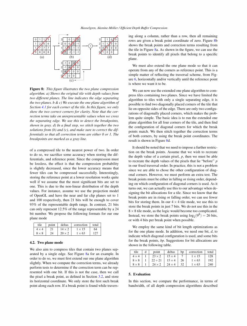
Figure 8: This figure illustrates the two plane compressionalgorithm. a) Shows the original tile with depth values fromtwo different planes. The line indicates the edge separatingthe two planes. b & c) We execute the one plane algorithm ofSection 4.1 for each corner of the tile. In this figure, we onlyshow the two correct corners for clarity. Note that the cor-rection terms take on unrepresentable values when we crossthe separating edge. We use this to detect the breakpoints,shown in gray. d) In a final step, we stitch together the twosolutions from (b) and (c), and make sure to correct the dif-ferentials so that all correction terms are either 0 or 1. Thebreakpoints are marked as a gray line.

of a compressed tile to the nearest power of two. In orderto do so, we sacrifice some accuracy when storing the dif-ferentials, and reference point. Since the compression mustbe lossless, the effect is that the compression probabilityis slightly decreased, since the lower accuracy means thatfewer tiles can be compressed successfully. Interestingly,storing the reference point at a lower resolution works quitewell if we assume that the most significant bits are set toone. This is due to the non-linear distribution of the depthvalues. For instance, assume we use the projection modelof OpenGL and have the near and far clip planes set to 1and 100 respectively, then 21 bits will be enough to cover93% of the representable depth range. In contrast, 21 bitscan only represent 12.5% of the range representable by a 24bit number. We propose the following formats for our oneplane mode

tile point deltas correction total4×4 21 14×2 1×15 648×8 24 20×2 1×63 127

4.2. Two plane mode

We also aim to compress tiles that contain two planes sep-arated by a single edge. See Figure 8a for an example. Inorder to do so, we must first extend our one plane algorithmslightly. When we compute the correction terms, we alreadyperform tests to determine if the correction term can be rep-resented with one bit. If this is not the case, then we callthe pixel a break point, as defined in Section 3.2, and storeits horizontal coordinate. We only store the first such breakpoint along each row. If a break point is found while travers-

ing along a column, rather than a row, then all remainingrows are given a break point coordinate of zero. Figure 8bshows the break points and correction terms resulting fromthe tile in Figure 8a. As shown in the figure, we can use thebreak points to identify all pixels that belong to a specificplane.

We must also extend the one plane mode so that it canoperate from any of the corners as reference point. This is asimple matter of reflecting the traversal scheme, from Fig-ure 6, horizontally and/or vertically until the reference pointis where we want it to be.

We can now use the extended one plane algorithm to com-press tiles containing two planes. Since we have limited thealgorithm to tiles with only a single separating edge, it ispossible to find two diagonally placed corners of the tile thatlie on opposite sides of the edge. There are only two configu-rations of diagonally placed corners, which makes the prob-lem quite simple. The basic idea is to run the extended oneplane algorithm for all four corners of the tile, and then findthe configuration of diagonal corners for which the breakpoints match. We then stitch together the correction termsof both corners, by using the break point coordinates. Theresult is shown in Figure 8d.

It should be noted that we need to impose a further restric-tion on the break points. Assume that we wish to recreatethe depth value of a certain pixel, p, then we must be ableto recreate the depth values of the pixels that lie “before” pin our fixed traversal order. In practice, this is not a problemsince we are able to chose the other configuration of diag-onal corners. However, we must perform an extra test. Thebreak points must be either in falling or rising order, depend-ing on which configuration of diagonal corners is used. As itturns out, we can actually use this to our advantage when de-signing the bit allocations for a tile. Since we know that thebreak points are in rising or falling order, we can use fewerbits for storing them. In our 4× 4 tile mode, we use this tostore the break points in just 7 bits. We do not use this in the8×8 tile mode, as the logic would become too complicated.Instead, we store the break points using log2(9

8) = 26 bits,or with 4 bits per break point when possible.

We employ the same kind of bit length optimizations asfor the one plane mode. In addition, we need one bit, d, toindicate which diagonal configuration is used, and some bitsfor the break points, bp. Suggestions for bit allocations areshown in the following table.

tile d point deltas bp correction total4×4 1 23×2 15×4 7 1×15 1288×8 1 22 + 21 15×4 26 1×63 1928×8 1 24×2 24×4 32 1×63 240

5. Evaluation

In this section, we compare the performance, in terms ofbandwidth, of all depth compression algorithms described


Average #Pixels Per Triangle

SponzaGame Scene 2Game Scene 1

160 x 1200.6

320 x 2402.4

640 x 4809.0

1280 x 102437.6

Average #Pixels Per Triangle160 x 120

3.0320 x 240

11.6640 x 480

45.41280 x 1024

194.1

Average #Pixels Per Triangle160 x 120

10.8320 x 240

41.6640 x 480

161.41280 x 1024

683.5

160 x 120 320 x 240 640 x 480 1280 x 10240

0.1

0.2

0.3

0.4

0.5

0.6

0.7

0.8

0.9

18 x 8 pixel tiles

Resolution

Com

pres

sion

ratio

Raw 8x8DDPCMPlane encodingDepth offset 8x8Our 8x8

160 x 120 320 x 240 640 x 480 1280 x 10240

0.1

0.2

0.3

0.4

0.5

0.6

0.7

0.8

0.9

14 x 4 pixel tiles

Resolution

Com

pres

sion

ratio

Raw 4x4AnchorPlane & depth offsetDepth offset 4x4Our 4x4

160 x 120 320 x 240 640 x 480 1280 x 10240

0.1

0.2

0.3

0.4

0.5

0.6

0.7

0.8

0.9

14x4 pixel tiles: compression relative to Raw8x8

Resolution

Com

pres

sion

ratio

Raw 4x4AnchorPlane & depth offsetDepth offset 4x4Our 4x4

Figure 9: The first row shows a summary of the benchmark scenes. The diagrams in the second row show the average compres-sion for all three scenes as a function of rendering resolution, for 4×4 and 8×8 pixel tiles. Finally, we show the depth bufferbandwidth of 4×4 tiles, relative to the bandwidth of a Raw 8x8 depth buffer. It should be noted that this diagram does not taketile table bandwidth into account.

in this paper. The tests were performed using our functionalsimulator, implementing a tiled rasterizer that traverses tri-angles a horizontal row of tiles at a time. We matched thetile size of the rasterizer to the tile size of each depth bufferimplementation in order to maximize performance for allcompression algorithms. Furthermore, we assumed a 64 bitwide memory bus, and accordingly, all our implementationsof compressors have been optimized to make the size of allmemory accesses aligned to 64 bits.

The depth buffer system in our functional simulator im-plements all features described in Section 2. We used a depthtile cache of approximately 2 kB, and full precision z-minand z-max culling. Our tests show that compression rates areonly marginally affected by the cache size.‡ Similarly, the z-min and z-max culling avoids a given fraction of the depthtile fetches, independent of compression algorithm. There-fore, it should affect all algorithms equally, and not affectthe trend of the results.

Most of the compression algorithms have two operational

‡ The efficiency of all algorithms increased slightly, and equally,with a bigger cache. We tested cache sizes of 0.5, 1, 2 and 4 kb

modes. Therefore, we have chosen this as our target. Further-more, two modes fit well into a two bit tile-table assumingwe also need to flag for uncompressed tiles and for fast zclears. It is our opinion that using fast clears makes for afair comparison of the algorithms. All algorithms can eas-ily handle cleared tiles, which means that our compressorswould be favored if this mode was excluded since they havethe lowest bit rate.

We evaluate the following compression configurations

• Raw 4x4/8x8: No compression.• DDPCM: The one and two-plane mode (not using “es-

cape codes”) of the DDPCM compression scheme fromSection 3.2, 8× 8 pixel tiles. Bit rate: 3/5 bpp (bits perpixel)

• Anchor: The anchor encoding scheme (Section 3.3), 4×4pixel tiles. Note that this is the only compression schemein the test that only uses one compression mode. One bit-combination in the tile table was left unused. Bit rate: 8bpp.

• Plane encoding: Van Hook’s plane encoding mode fromsection 3.4, 8×8 pixel tiles. Only the two and four planemodes were used, since we only allow 2 compressionmodes. This algorithm was given a slight favor in formof a 16.6% bigger depth tile cache. Bit rate: 4/7 bpp.


• Plane & depth offset: The plane (Section 3.4) and depthoffset (Section 3.5) encoding modes of Orenstein et al,4× 4 pixel tiles. Bit rate: 8/16 bpp, 8 bits for the planemode and 16 bits for the depth offset mode.

• Depth Offset 4x4/8x8: Morein and Natale’s depth offsetcompression mode from Section 3.5. We used two com-pression modes, one using 12 bit offsets, and one with 16bit offsets. Bit rate: 12/16 bits per pixel for both 4×4 and8×8 tiles.

• Our 4x4/8x8: Our compression scheme, described in Sec-tion 4. For the 8×8 tile mode, we used the 192 bit versionof the two plane mode in this evaluation. Bit rate: 4/8 bitsper pixel for 4× 4 tiles and 2/3 bits per pixel for 8× 8tiles.

Our benchmarks were performed on three differenttest scenes, depicted in Figure 9. Each test scene fea-tures an animated camera with static geometry. Further-more, we rendered each scene at four different resolutions:160×120,320×240,640×480, and 1280 × 1024 pixels.Varying the resolution is a simple way of simulating dif-ferent levels of tessellation. As can be seen in Figure 9, wecover scenes with great diversity in the average triangle area.

In the bottom half of Figure 9, we show the compressionratio of each algorithm, grouped into algorithms for 4× 4and 8×8 pixel tiles. We also present the compression of the4× 4 tile algorithms, as compared to the bandwidth of theRaw 8x8 mode. It should be noted that this relative com-parison only takes the depth buffer bandwidth into account.Thus, the bandwidth to the tile table will increase as the tilesize decrease. How much of an effect this will have on thetotal bandwidth, will depend on the format of the tile table,and on the efficiency of the culling.

For 8× 8 pixel tiles, our algorithm is the clear winneramong the algorithms supporting high resolution interpo-lation, but it cannot quite compete with Van Hook’s planeencoding algorithm. This is not very surprising consideringthat the plane encoding algorithm is favored by a slightlybigger depth tile cache, and avoids correction terms by im-posing the restriction that depth values must be interpolatedin the same resolution that is used for storage.

For 4× 4 pixel tiles, the advantages of our algorithm be-comes really clear. It is capable of bringing the two-planeflexibility that is only seen in the 8×8 tile algorithms downto 4×4 tiles, and still keeps a reasonably low bit rate. A twoplane mode for 4× 4 tiles is equal to having the flexibilityof eight planes (with some restrictions) in an 8×8 pixel tile.This shows up in the evaluation, as our 4×4 tile compressionmodes have the best compression ratio at all resolutions.

6. Conclusions

We hope that our survey of previously existing depth buffercompression schemes will provide a valuable source for thegraphics hardware community, as these algorithms have not

been presented in an academic paper before. As we haveshown, our new compression algorithm provides competi-tive compression for both 4× 4 and 8× 8 pixel tiles at var-ious resolutions. We have avoided an exhaustive evaluationof whether 4× 4 or 8× 8 tiles provide better performance,since this is a very difficult undertaking which depends onseveral other parameters. Our work here has been mostly onan algorithmic level, and therefore, we leave more detailedhardware implementations for future work. We are certainthat this is important, since such implementations may re-veal other advantages and disadvantages of the algorithms.Furthermore, we would like to examine how to best deal withdepth buffer compression of anti-aliased depth data.

AcknowledgementsWe acknowledge support from the Swedish Foundation for Strate-gic Research and Vetenskapsrådet. Thanks for Jukka Arvo and PetriNordlund of Bitboys for providing input.

References

[AMS03] AKENINE-MÖLLER T., STRÖM J.: Graphics forthe Masses: A Hardware Rasterization Architecture for MobilePhones. ACM Transactions on Graphics, 22, 3 (2003), 801–808.

[DMFW02] DEROO J., MOREIN S., FAVELA B., WRIGHT M.:Method and Apparatus for Compressing Parameter Values forPixels in a Display Frame. In US Patent 6,476,811 (2002).

[GKM93] GREENE N., KASS M., MILLER G.: Hierarchical Z-Buffer Visibility. In Proceedings of ACM SIGGRAPH 93 (Au-gust 1993), ACM Press/ACM SIGGRAPH, New York, J. Kajiya,Ed., Computer Graphics Proceedings, Annual Conference Series,ACM, pp. 231–238.

[MN04] MOREIN S., NATALE M.: System, Method, and Appa-ratus for Compression of Video Data using Offset Values. In USPatent 6,762,758 (2004).

[Mor00] MOREIN S.: ATI Radeon HyperZ Technology. In Work-shop on Graphics Hardware, Hot3D Proceedings (August 2000),ACM SIGGRAPH/Eurographics.

[Mor02] MOREIN S.: Method and Apparatus for Efficient Clear-ing of Memory. In US Patent 6,421,764 (2002).

[MWY03] MOREIN S., WRIGHT M., YEE K.: Method and appa-ratus for controlling compressed z information in a video graph-ics system. US Patent 6,636,226, 2003.

[OPS∗05] ORNSTEIN D., PELED G., SPERBER Z., COHEN E.,MALKA G.: Z-Compression Mechanism. In US Patent 6,580,427(2005).

[SSS74] SUTHERLAND E. E., SPROULL R. F., SCHUMACKER

R. A.: A characterization of ten hidden-surface algorithms. ACMComput. Surv. 6, 1 (1974), 1–55.

[Van03] VAN HOOK T.: Method and Apparatus for Compressionand Decompression of Z Data. In US Patent 6,630,933 (2003).

[VM05] VAN DYKE J., MARGESON J.: Method and Apparatusfor Managing and Accessing Depth Data in a Computer GraphicsSystem. In US Patent 6,961,057 (2005).

efficient depth buffer compression

Documents