efficient credit policies in a housing debt crisis · efficient credit policies in a housing debt...
TRANSCRIPT

73
Janice eberlyNorthwestern University
arvind KrishnamurthyStanford University
Efficient Credit Policies in a Housing Debt Crisis
ABSTRACT Consumption, income, and home prices fell simultaneously during the financial crisis, compounding recessionary conditions with liquidity constraints and mortgage distress. We develop a framework to guide govern-ment policy in response to crises in cases when government may intervene to support distressed mortgages. Our results emphasize three aspects of efficient mortgage modifications. First, when households are constrained in their bor-rowing, government resources should support household liquidity up-front. This implies modifying loans to reduce payments during the crisis rather than reducing payments over the life of the mortgage contract, such as via debt reduction. Second, while governments will not find it efficient to directly write down the debt of borrowers, in many cases it will be in the best interest of lenders to do so, because reducing debt is an effective way to reduce strategic default. Moreover, the lenders who bear the credit default risk have a direct incentive to partially write down debt and avoid a full loan loss due to default. Finally, a well-designed mortgage contract should take these considerations into account, reducing payments during recessions and reducing debt when home prices fall. We propose an automatic stabilizer mortgage contract which does both by converting mortgages into lower-rate adjustable-rate mortgages when interest rates fall during a downturn—reducing payments and lowering the present value of borrowers’ debt.
during the financial crisis and in its aftermath, those segments of the economy most exposed to the accumulation of mortgage debt have
tended to fare the worst. Whether one measures the impact by industry (construction), by geography (sand states), or by household (the most indebted), the presence of greater mortgage debt has led to weaker economic

74 Brookings Papers on Economic Activity, Fall 2014
outcomes (see, for example, Mian and Sufi 2009 and Dynan 2012). More-over, research suggests that financial crises may be more severe or may be associated with slower recoveries when accompanied by a housing col-lapse (Reinhart and Rogoff 2009; Howard, Martin, and Wilson 2011; and International Monetary Fund 2012).
These observations lead to an apparently natural macroeconomic policy prescription: restoring stronger economic growth requires reducing accu-mulated mortgage debt. In this paper, we consider this proposal in an envi-ronment where debt is indeed potentially damaging to the macroeconomy and where the government and private sector have a range of possible policy interventions. We show that while debt reduction can support eco-nomic recovery, other interventions can be more efficient. We also show that whether debt reduction is financed by the government or by lenders matters for both its efficacy and its desirability. Hence, while the intuitive appeal of debt reduction is clear, its policy efficiency is not always clear, and the argument is more nuanced than the simple intuition.
Our results emphasize three aspects of efficient mortgage modifications. First, when households are borrowing-constrained, government support should provide liquidity up-front. This implies loan modifications that reduce payments during the crisis, rather than using government resources for debt reduction that reduces payments over the life of the mortgage con-tract. The reasoning behind this result is simple and robust. Consider choos-ing among a class of government support programs, all of which transfer resources to a borrower, but which may vary in the timing of transfers. Sup-pose the objective of the program is to increase the current consumption of the borrower. For a permanent-income household, only the present dis-counted value of the government transfers matters for current consumption. But for a liquidity-constrained household, for any given present discounted value of transfers, programs that front-load transfers increase consumption by strictly more. Thus, up-front payment reduction is a more efficient use of government resources than debt reduction.
Second, while governments will not find it efficient to directly write down borrower debt, in many cases it will be in the best interest of lenders to do so. Reducing debt is effective in reducing strategic default. Lend-ers, who bear the credit default risk, have a direct incentive to partially write down debt and avoid greater loan losses due to default. In cases where there are externalities from default that will not be internalized by the lender, government policy can be effective in providing incentives or systematic structures to lenders to write down debt. Finally, a well-designed mortgage contract should take these considerations into account ex ante,

Janice eberly and arvind Krishnamurthy 75
reducing payments during recessions and reducing debt when home prices fall. We propose an automatic stabilizer mortgage contract which does both by converting mortgages into lower-rate adjustable-rate mortgages when interest rates fall during a downturn—reducing payments and lowering the value of borrowers’ debt.
We begin with a simple environment with homeowners, lenders, and a government. We start from the simplest case, namely one with perfect information where all households are liquidity constrained. We then layer on default, private information, heterogeneous default costs, endogenous provision of private mortgage modifications by lenders, and an equilibrium home price response.
Initially, homeowners may consider defaulting on their mortgages because they are liquidity constrained (that is, cash-flow constrained) or because their mortgages exceed the value of their homes (strategic default), or because both considerations may be present. The government has finite resources and maximizes utility in the planner’s problem. We initially consider a two-period model with exogenous home prices and then allow for general equilibrium feedback. We ask, “What type of intervention is most effective, taking into account the government budget constraint and the program’s effectiveness at supporting the economy?” We consider a general class of interventions that includes mortgage modifications, such as interest rate reductions, payment deferral, and term extensions, as well as mortgage refinancing and debt write-downs. We extend the model to include default with known, uncertain, and unobserved default costs, with dynamic default timing, and with lender renegotiation.
The model is abstract and simple by design, allowing us to focus on the minimum features necessary to highlight these mechanisms in the hous-ing market. It omits many interesting and potentially relevant features of the housing market and of the economy more generally. For example, we generate a “crisis period” exogenously by specifying lower income in one period to disrupt consumption smoothing by households. We could, in principle, embed our housing model in a general equilibrium frame-work that would derive lower income and generate the scope for housing policy endogenously, as in the studies done by Gauti Eggertson and Paul Krugman (2010), Robert Hall (2010), Veronica Guerrieri and Guido Lorenzoni (2011), Emmanuel Farhi and Ivan Werning (2013), and others. For example, in the work by Eggertson and Krugman, the nominal values of debt and sticky prices, along with the liquidity-constrained households that we include, cause output to be determined by demand; hence there is scope for policy to improve macroeconomic outcomes when the debt constraint

76 Brookings Papers on Economic Activity, Fall 2014
binds and the nominal interest rate is zero. Including our model in such a structure would also allow us to examine how housing policy feeds back into the macroeconomy from the housing market. While this would be an interesting route to pursue, our focus is on distinguishing between various types of housing market interventions, so the additional impact that may come from the macroeconomic feedback is left for further work.
Here the crisis period is defined by low income, which constrains con-sumption due to liquidity constraints. The household cannot borrow against future income nor against housing equity in order to smooth through the crisis. The government has a range of possible policy interventions and a limited budget; we focus on policies related to housing modifications, given the severity of the constraints and defaults experienced there. For simplicity, we begin with a case without default. The main result that comes from analyzing this case is that the need for consumption smoothing favors transfers to liquidity-constrained households during the crisis period. Optimally, such transfers will take the form of a payment deferral, granting resources to the borrower in a crisis period in return for repayment from the borrower in a noncrisis period. We then add the potential for default and show that optimal policies that concentrate transfers early in the crisis but require repayment later may lead to defaults.
These results suggest that payment deferral policies alone (which grant short-term reductions in home payments but are repaid with higher loan balances later), may generate payments that rise too quickly and gener-ate defaults, suggesting that payment forgiveness to replace or augment payment deferrals may be optimal. That is, government resources should first be spent on payment forgiveness. Once the resource allocation is exhausted, further modifications should take the form of payment deferral. We also show that “debt overhang” concerns, that is, the possibility that debt inhibits access to private credit and reduces consumption, do not change our results. Even if loan modifications such as principal reduction reduce debt overhang, liquidity constraints can be directly and more effi-ciently addressed by front-loaded policy interventions, rather than through a reduction in contracted debt.
We study the borrower’s incentive to “strategically” default in the crisis period. We find that in many cases borrowers will choose to service an underwater mortgage. They do so for two reasons. First, default involves deadweight costs which the borrower will try to avoid. Second, when borrowers can choose when to default—either during a crisis or later—they will value the option to delay default and instead continue to service an underwater mortgage. In this context, payment reduction will have a more

Janice eberly and arvind Krishnamurthy 77
beneficial effect than principal reduction in supporting consumption. We also show that payment reduction increases the incentive to delay a default and thus reduces foreclosures in a crisis.
While government resources are best spent on payment reduction, a lender may find it preferable to write down debt. Since lenders bear the credit default risk, effectively they fully write down the loan (and take back the collateral) if it defaults. Hence, renegotiating the loan, including partially writing down debt to avoid strategic default, can be in the lender’s own best interest. However, lenders also tend to delay in order to preserve the option value of waiting, since the loan may “cure” without any inter-vention. Without liquidity constraints, lenders concerned about strategic default would optimally offer a debt reduction at the end of the period (defined as just prior to default) in order to preserve option value but avoid costly default. When there are externalities from default that will not be internalized by the lender, government policy can still play a useful role, in this case by providing lender incentives to write down debt.
Summarizing, our analysis of loan modifications produces two broad results. First, with liquidity constraints, transfers to households during the crisis period weakly dominate transfers at later dates and hence are a more effective use of government resources. These initial transfers could include temporary payment reductions, such as interest rate reductions, payment deferrals, or term extensions. This result is robust to including default, vari-ous forms of deadweight costs of default, debt overhang, and the easing of credit constraints through principal reduction. Generally, any policy that transfers resources later can be replicated by an initial transfer of resources, although the converse is not true. Second, principal reductions should be offered by lenders and not by the government. Principal reductions can reduce any deadweight costs due to strategic default. This conclusion is independent of whether or not liquidity constraints are present. Lend-ers have a private incentive to write down debt since they bear losses in default, so writing down debt can increase the value of the loan to lenders. With the potential for delay, however, lenders will find it privately optimal to delay debt write-downs until just prior to default.
Allowing for endogenous price determination in the housing market reinforces these results. We embed the consumption and policy choice problem in an equilibrium model of housing, with rental housing demand augmented by households defaulting on their mortgages and moving from homeownership to rental. The key result from this section is that fore-closures by liquidity-constrained households undermine home-purchase demand and hence prices more than strategic defaults do. Any default

78 Brookings Papers on Economic Activity, Fall 2014
incurs the deadweight cost of default, so this (potentially large) cost is the same regardless of the cause of the default. However, liquidity-constrained households carry their constraint into the rental market, which constrains their housing demand and puts further downward pressure on home prices. Strategic defaulters, on the other hand, are not in liquidity distress by defi-nition and hence have greater demand for housing than do the liquidity-constrained. For a policymaker concerned about foreclosure externalities and home prices, distressed foreclosures by liquidity-constrained house-holds are more damaging.
Our results demonstrate that different types of ex post interventions in home lending solve conceptually distinct problems. For example, payment-reducing modifications, which steepen the profile of payments through payment deferrals, temporary interest rate reductions, or term extensions, address cash flow and liquidity constraints. Loan principal reductions are inefficient at addressing cash flow issues, because they backload payment reductions, but they are effective at addressing the risk of strategic defaults in the later period (though not the initial period) that lenders face.
These results on ex post modifications are suggestive of the ex ante properties of loan contracts that would ameliorate the problems that arise during a crisis with both borrowing constraints and declining home prices. Specifically, a contract should allow for lower payments when borrow-ing constraints bind and a reduction in loan obligations when home prices fall to reduce the incentive for strategic default. Such a contract fills the role of automatic stabilizers in the housing market by responding to eco-nomic conditions. An automatic stabilizer mortgage contract that includes a reset option—that is, that can be reset as a lower-adjustable-rate mort-gage during a crisis period—is consistent with the ex ante security design problem. The cyclical movement of interest rates is key to achieving the state-contingency: if the central bank reduces rates during cyclical down-turns and when home prices fall, the reset option allows mortgage borrow-ers to reduce their payments in a recession as well as their outstanding debt. This latter effect on debt reduction occurs because a reduction in contract interest rates via a reset option reduces the present value of the payment stream owed by the borrower. This present value of payments, rather than a contracted face amount of principal, is the critical variable that enters a strategic default decision. Finally, since it relies on a reset option that is quite similar to the standard refinancing option, such a contract is also near the space of existing contracts with pricing expertise and scale.
Various forms of home price insurance or indexing of contracts to home prices have been proposed (for example, see Mian and Sufi 2014) to address

Janice eberly and arvind Krishnamurthy 79
the problems posed by negative equity. These options also implement the intent to avoid strategic default in a downturn. Some contracts of this type have been implemented on a small scale, although measuring home prices at the appropriate level of aggregation and allowing for home improve-ments and maintenance incentives pose practical challenges. Indexing to interest rates, as suggested in the stabilizing contract, has the advantages of being observable and consistent and preserving monetary policy effective-ness. Contracts with this feature already exist and have been implemented and priced on a large scale. Moreover, effectively indexing contracts to interest rates makes them sensitive to a broader range of economic condi-tions than home prices alone.
The remainder of this paper is organized as follows. The next section lays out a basic two-period model in which a household takes on a mort-gage to finance both housing and nonhousing consumption. We then shock the household’s income in a crisis period and study the optimal form of transfer that smooths household consumption, showing that it takes the form of a mortgage payment deferral. In section II we introduce the pos-sibility that the household may default on the mortgage at the final period because the mortgage is underwater (a strategic default). Since payment deferral increases the incidence of strategic default, the optimal mortgage modification includes more crisis-period payment reduction and less defer-ral. In section III, we study the case where the borrower may strategically default in the crisis period as well as the final period. We find that borrowers may delay defaulting in a crisis period because the option to delay is valu-able. In this context, our earlier results concerning the merits of payment reduction over principal reduction are strengthened. In section IV, we study the lender’s incentives to modify mortgages. We show that lenders, unlike the government, will find it efficient to reduce mortgage principal, but only just before the borrower defaults. In section V, we consider the question of why there were so few modifications in practice during the recession, and show that one reason may be adverse selection. With the possibility of pri-vate information, lenders will be concerned that a given modification will only attract types of borrowers that cause them to make negative profits. We show that this consideration can cause the modification market to break down. In section VI, we embed our model in a simple housing market equilibrium and show that the merits of spending government resources on payment reduction rather than principal reduction are strengthened by general equilibrium considerations. In section VII, we turn to the ex ante contract design problem and suggest that a mortgage contract that gives the borrower the right to reset the mortgage rate into a variable-rate

80 Brookings Papers on Economic Activity, Fall 2014
mortgage goes some way toward implementing the optimal contract. Section VIII concludes.
I. Basic Model
Households derive utility from housing and other consumption goods according to the consumption aggregate, Ct:
( ) ( )≡ ( )α −α(1) ,1C c ct th
t
where cht is consumption of housing services and ct is consumption of non-
housing goods. The household maximizes linear utility over two periods
= +(2) ,1 2U C C
where we have set the discount factor to 1, since it plays no role in the analysis.
At date 0, that is, a date just prior to date 1, the household purchases a home and takes out a mortgage loan. At the date 0 planning date, the household expects to receive income of y at both dates. For now, there is no uncertainty. Income is allocated to nonhousing consumption and to pay-ing interest on a mortgage loan to finance housing consumption. A home of size ch costs P0 and is worth P2 at date 2. In the basic model, P2 is non-stochastic. (Later we will introduce home price and income uncertainty; for now, we take these as given and known to the household.) The home price P0 satisfies the asset pricing equation,
(3) ,0 2= + +P rc rc Ph h
where r is defined as the per-period user cost of housing. That is, if an agent purchases a home for P0 and sells it in two periods for P2, the net cost over the two periods is 2rch (= P0 - P2).
To finance the initial P0 outlay, the household takes on a mortgage loan. A lender provides P0 funds to purchase the house in return for interest pay-ments of l1 and l2 and a principal repayment of D. For the lender to break even, repayments must cover the initial loan:
(4) ,1 2 0+ + =l l D P
where we have set the lender’s discount rate to 1, as well. Given choices of (l1, l2, D), nonhousing consumption is

Janice eberly and arvind Krishnamurthy 81
(5) and, .1 1 2 2 2= − = + − −c y l c y P D l
The household chooses (l1, l2, D) to maximize (2).It is straightforward to derive the result that a consumption-smoothing
household maximizes utility by setting
(6) and, .1 2 2= = α =l l y D P
That is, interest payments on the housing loan are ay, and the principal repayment is made by selling the home for P2. These choices result in consumption
(7) and, 1 .( )= α = − αcy
rc yt
ht
Note that with Cobb-Douglas preferences, the expenditure shares on hous-ing and nonhousing consumption are a and 1 - a. Since the effective user cost of housing, r, is constant over both periods, the household equalizes consumption over both dates.1
I.A. Crisis
A “crisis” occurs in the model by allowing an unanticipated negative income shock to hit this household, so that income at date 1 is instead y1 < y, leaving income at date 2 unchanged. There are two ways the household can adjust to this shock. It can default on the mortgage, reduce housing consumption, and increase nonhousing consumption.2 Alternatively, it can borrow from date 2, reducing future consumption and increasing current consumption. We first study the second option and assume that the house-hold does not default on its mortgage (we will consider default in the next sections). If the household does not default, it will consume too little of nonhousing services at date 1, both because permanent income is lower and also because the household cannot smooth nonhousing consumption by borrowing against future income, so that
c c<(8) .1 2
1. With linear utility, the consumption allocation is formally indeterminate, but any amount of curvature will produce consumption smoothing in this way.
2. In principle, the household could sell the home and buy another to reoptimize con-sumption. We assume that this is costly or not feasible as a way of smoothing consumption for temporary shocks. We discuss borrowing further below.

82 Brookings Papers on Economic Activity, Fall 2014
That is, if the household could borrow freely at an interest rate of zero, it would increase date 1 consumption and reduce date 2 consumption.
A household with other assets, or one with equity in its home, can bor-row to achieve this optimum consumption path. We instead will focus on a liquidity-constrained household. This household has no other assets, little to no equity in the home, and is unable to borrow against future income.3 Hence this household can only adjust its nonhousing consumption beyond the liquidity constraint by defaulting on its mortgage, since it cannot bor-row against future income or consume from other assets or home equity.4 If it does not default, then date 1 consumption is constrained by the precom-mitted mortgage payment.
Let us suppose that a government has Z dollars that it can spend to increase household utility. The scope for government intervention arises in this setting directly because of the liquidity constraint, as in Eggertson and Krugman (2010) and Guerreri and Lorenzoni (2011), or due to other nominal rigidities, as in Farhi and Werning (2013) and others. It could also be reinforced by an aggregate demand shortfall, consumption externalities, other credit market frictions, or other considerations. We do not model these explicitly, since our focus is on the housing market (although we allow for additional considerations in the next sections). Hence, the government’s budget allocation may result from its intention to ease liquidity constraints in period 1, or similarly, as a way of implementing countercyclical macro-economic policies, since date 1 is the “crisis” period in the model.
Suppose the government chooses transfers to households (t1, t2) in the first and second period, respectively, that satisfy the budget constraint5
(9) .1 2+ =t t Z
Various choices of t1 and t2 can be mapped into standard types of loan modifications. For example, setting t1 > 0 and t2 = 0 in our notation
3. In principle, the household could also sell the home and use the proceeds to buy a new one, reoptimizing over the two types of consumption. This means that the household is effec-tively not liquidity constrained, since the home becomes a liquid asset. We assume that this option is not available to the household, either because transaction costs are high, the home is underwater and the household has insufficient other assets (so that a home sale—a short sale—would require a loan default), or credit market frictions prevent the homeowner from consuming out of real estate wealth.
4. The importance of liquidity constraints during the crisis is emphasized in the empirical results of Dynan (2012) using household consumption data.
5. Note that the government’s discount rate is also 1, so we do not give the government an advantageous borrowing rate compared to private agents.

Janice eberly and arvind Krishnamurthy 83
corresponds to a pure “payment reduction” loan modification, which temporarily reduces loan payments, for example through a temporary interest rate reduction. A “payment deferral” program offsets the initial payment reduction with future payment increases, setting t1 > 0 and t2 < 0, for example through a maturity extension or loan forbearance. A pro-gram with t1 = t2 > 0, so that payment reductions are equally spread over time, corresponds to a fixed-rate loan refinancing (since loan payments are lowered uniformly) and to principal reduction, that is, a reduction in the loan principal that results in reduced interest and principal payments at each date.
With these transfers, the household’s budget set is now augmented by a transfer in period 1 to help overcome the liquidity constraint and a second transfer at date 2, resulting in household consumption of
= − α + = − α +c y y t c y y t(10) , .1 1 1 2 2
Here we consider only policies related to modifying the mortgage; in the next section, we add default so that policies are more directly tied to mort-gage payments. The planner maximizes household utility
( ) ( ) ( ) ( )+( ) ( )α −α α −αc c c ct t
h h(11) max ,1 1
1
2 2
1
1, 2
subject to equations 9 and 10. Note that since we are considering the case where the household does not default and hence does not reoptimize hous-ing consumption, the consumption values c c ⁄rh h
1 2, = yα , are invariant to the choice of t1 and t2.
We can rewrite the planner’s problem thus:
v y y t v y t s t t t Zt t
( ) ( )( )− α + + − α + + =(12) max 1 . . ,1 1 2 1 21, 2
where
(13) 1( )( ) ( )≡ α α−αv c
y
rct t
and we note that v (z) is concave. This problem provides the minimal incen-tive to support household consumption, as it focuses only on the liquidity constraint of a single household and does not take into account aggregate demand externalities that may be present in a crisis, as emphasized by other authors.

84 Brookings Papers on Economic Activity, Fall 2014
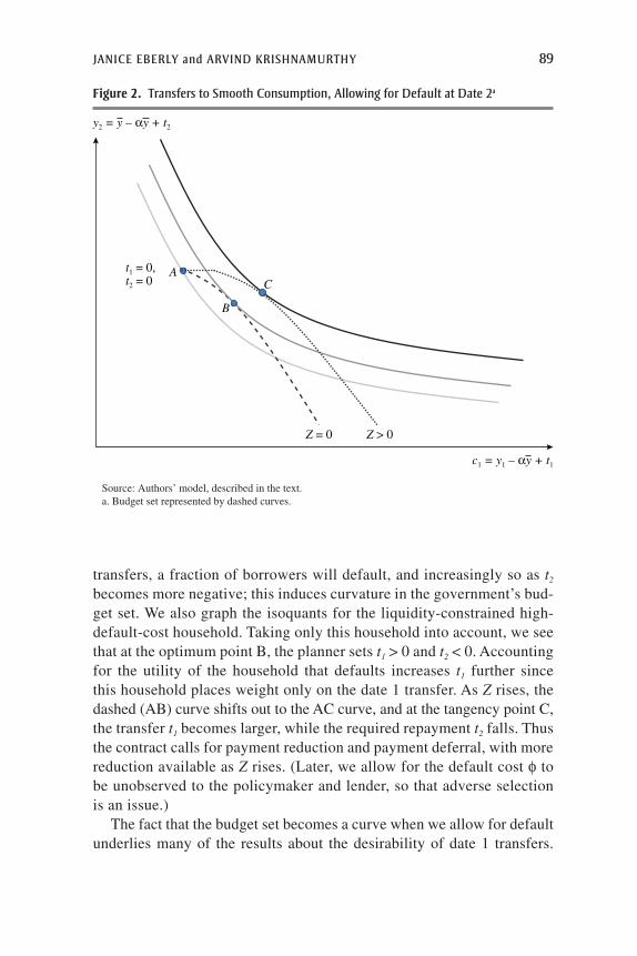
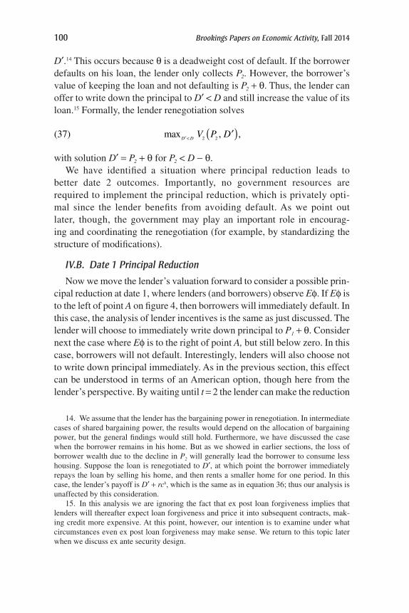
Figure 1 illustrates the solution for nonhousing consumption for Z = 0. The vertical axis graphs c2, while the horizontal axis graphs c1. The initial point A after the shock has c2 > c1. The bold diagonal line traces out the set of points that satisfy the budget constraint, t1 + t2 = 0 (that is, Z = 0). The optimum calls for full consumption smoothing, which is to set t1 > 0 and t2 < 0 until c1 = c2 (the dotted 45-degree line) at point B.
As Z rises, the bold diagonal line shifts outward, but for any given Z we see that payment deferral (t1 > 0, t2 < 0) is better than payment reduction (t1 > 0, t2 = 0) because it allows higher transfers in the first period, which is in turn better than principal reduction (t1 > 0, t2 > 0), where transfers con-tinue beyond the crisis period. This finding is consistent with general results in public finance showing that transfers into liquidity-constrained states enhance utility, since the marginal utility of consumption is high in those states. A reduction in mortgage principal does not transfer liquid assets into those states since the household is by definition liquidity-constrained and
Figure 1. Consumption Smoothing with Date 1 and Date 2a Transfers and No Default
45°
Source: Authors’ model, described in the text.a. Transfer at date 1 signified by t
1; transfer at date 2 signified by t
2.
c2 = y – αy + t2
c1 = y1 – αy + t1
t1 = 0,t2 = 0
t1 > 0, t2 < 0
A
B

Janice eberly and arvind Krishnamurthy 85
cannot borrow against its higher wealth. The increase in wealth is imple-mented by a stream of lower mortgage payments over the life of the loan, which is likely to extend well beyond the crisis period. Hence, gathering those benefits together into a front-loaded transfer is more effective. We highlight this result in this simplest setting because it is robust throughout as we add additional features to the model: transfers in the initial crisis period at least weakly dominate policies that transfer resources later.
We have described the solution (t1 and t2) as the solution to the planning problem. However, there is nothing in our setup thus far that precludes the private sector from offering a loan modification. If private lenders could offer contracts with t1 > 0, t2 < 0 they would find it profitable to do so. This would correspond to loan refinancing with term extension, for example, which might be desirable to households by reducing payments immedi-ately but also profitable for lenders over the life of the loan. Nonetheless, there are several reasons why policy may still be desirable. While we have not modeled a government’s preference for countercyclical policy, private lenders might not offer the socially optimal amount of modifications if there are credit market frictions, consumption externalities, or an aggregate demand shortfall. Hence, it may be optimal for the government to offer or subsidize modifications in addition to available private sector contracts. Moreover, later we will show that with asymmetric information, the market in private contracts may collapse due to adverse selection, which provides further scope for policy intervention.
II. Optimal Decisions and Default Risk at Date 2
Without default, the best transfer policy is to reduce payments as much as possible in the crisis period in order to support consumption. Given the government’s budget constraint, a policy that reduces mortgage payments in the crisis period and defers the payments until date 2 is the most cost effective; that is, for a given budget, it allows the most payment reduc-tion during the crisis. However, in practice such loans may induce default by front-loading the benefits and back-loading the costs of the program to households. Households, especially those with underwater mortgages, may use the payment deferral and then subsequently default on the loan. In this section, we study the case where agents can reoptimize and possibly default at date 2, allowing us to examine how policy interventions at date 1 affect subsequent date 2 default. In section III, we consider the case where agents can reoptimize and default at either date 1 or date 2, so that there is a timing element in the default decision.

86 Brookings Papers on Economic Activity, Fall 2014
II.A. Stochastic Home Price, Date 2 Decisions, and Default
Suppose that at the start of date 2 before the household consumes or makes interest payments on debt, the home price P2 changes. Agents then have the opportunity to reoptimize their consumption and borrow-ing choices, possibly defaulting on their mortgage loan. The home price change is unanticipated from the date 0 perspective. We analyze decisions at date 2, taking previous decisions as given.
At the start of date 2, prior to any interest payments or default decisions, a household has wealth of
(14) .2 2+ − +y P D t
If P2 - D + t2 ≠ 0, the household will want to rebalance consumption. For example, if P2 - D + t2 > 0, the household will want to increase housing and nonhousing consumption given that its wealth is greater than the ini-tially expected amount of y
_. We suppose that at date 2 the household can
readily sell the home, repay any debts, and be left with y_ + P2 - D + t2. The
household uses these resources to purchase (or rent) a home for one period. Given Cobb-Douglas preferences and a one-period user cost of housing of r, it is straightforward to show that utility over date 2 consumption is linear in wealth,
� ��� ���
y P t Dr( )( ) ( )+ + − α − α
ψα
−α(15) 1 ,2 21
where y is the marginal value of a dollar at date 2 and will be a constant throughout the analysis. If a household defaults on its mortgage, it loses the home, which was the collateral for the loan, and loses any equity in the home. Since the household still requires housing services, it enters the rental market to replace the lost housing services. The household also suffers a default cost, which may represent restricted access to credit mar-kets, benefits of homeownership or neighborhoods, match-specific benefits of the home, and so on. Thus, in default the household’s wealth becomes
− θy(16) ,
where q is a deadweight cost of default. Note that the household also loses the date 2 home-related transfer of t2. The household utility from this wealth is (y
_ - q)y. The household defaults if

Janice eberly and arvind Krishnamurthy 87
(17) ,2 2− θ > + − +y y P D t
so that wealth after defaulting exceeds wealth of continuing to service the mortgage.
Define the equity in the home (P2 - D) plus the default cost as
(18) ,2φ ≡ + θ −P D
which represents the total cost of default to the household. Then the default condition is expressed by the inequality
(19) ,2φ < −t
which determines whether the household defaults on its mortgage and incurs the deadweight cost of default. Otherwise the household continues to service the mortgage.
II.B. Optimal Date 1 Loan Modification with Date 2 Default Risk
We now solve for the optimal loan modification, accounting for the pos-sibility that some borrowers will default on their loans. Our principal con-clusion is that the payment reductions and deferrals still dominate principal reductions. Moreover, since default risk increases under payment defer-ral, because borrowers have to pay back more in the future, government resources are best spent first providing payment relief and only then shift-ing to payment deferral.
Suppose that f, which measures the incentive to default, is a random variable that is realized at date 2. For example, realizations of P2 may vary across homeowners, leading to different realizations of f. Moreover, sup-pose the possibility that home prices are uncertain only becomes apparent to borrowers and lenders at date 1. That is, continue to assume that this uncertainty is unanticipated at the date 0 stage, so that the date 0 loan con-tract is signed under the presumption that home prices are certain.
Default risk affects the planner’s decisions over (t1, t2) because the plan-ner has to account for the possibility that setting t2 < 0 (or requiring date 2 payments for borrowers) may induce default. Denote the CDF of f as F(f). Since borrowers default when f < -t2, for any given t2 we have F(-t2) bor-rowers defaulting on loans. We will assume the interesting case where (t1, t2) are such that it is advantageous for every liquidity-constrained bor-rower to take the modification contract, but a fraction F(-t2) strategically default on their loans in the second period.

88 Brookings Papers on Economic Activity, Fall 2014
A planner with Z dollars to spend solves thus:
( ) ( ) ( )
( ) ( ) ( )
[ ] [ ]
[ ]
− − − α + + + + − ψ φ > −
+ − − α + + − θ ψ φ < −
F t E v y y t y t P D t
F t E v y y t y t
t t(20) max 1
.
,2 1 1 2 2 2
2 1 1 2
1 2
The first line is the utility of the constrained borrowers with high default costs (that is, high f) who take the modification and do not default. The second line is the utility of the constrained borrowers who will default.
The government budget constraint requires6
( )[ ]− − − − =Z t F t t(21) 1 0.2 2 1
A fraction 1 - F (-t2) of borrowers make the repayment of -t2. This repay-ment plus the Z dollars must cover the initial payment of t1.
Denote µ as the Lagrange multiplier on the budget constraint. The first-order condition with respect to t1 gives
(22) ,1 1( )′ − α + = µv y y t
and with respect to t2 gives
( ) ( ) ( )[ ] [ ]{ }− − ψ = µ − − +F t F t t f t(23) 1 1 .2 2 2 2
Combining, we find
( ) ( )( )
[ ]′ − α + ψ = +− −
−v y tt f t
F t(24) 1 1
1.2
1 2 2
2
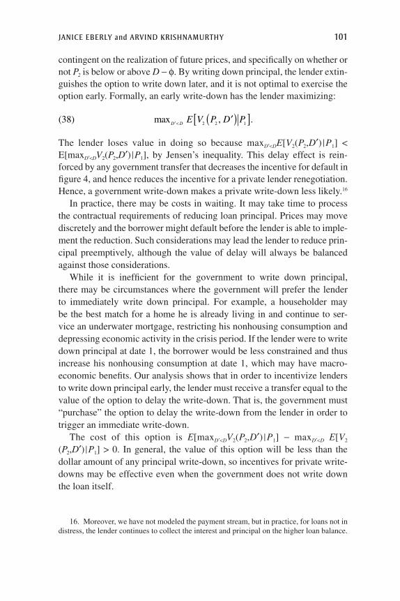
The solution is easy to illustrate pictorially. Figure 2 graphs first and second period nonhousing consumption for various values of govern-ment transfers. The curves AB and AC in figure 2 illustrate the set of all transfers that satisfy the government’s budget constraint. The key point is that this set is a “curve” for t1 > Z. Starting from point A, where trans-fers are zero, along the dashed curve, as t1 exceeds Z, -t2 must become negative to satisfy the budget constraint. However, with negative date 2
6. The budget constraint does not require that the program pay for itself unless Z = 0. If Z > 0, the program provides net funds for mortgage modifications, and date 1 payment reduc-tions can be larger to the extent that they are repaid at date 2 with negative transfers, t2 < 0.
Janice eberly and arvind Krishnamurthy 89
transfers, a fraction of borrowers will default, and increasingly so as t2 becomes more negative; this induces curvature in the government’s bud-get set. We also graph the isoquants for the liquidity-constrained high-default-cost household. Taking only this household into account, we see that at the optimum point B, the planner sets t1 > 0 and t2 < 0. Accounting for the utility of the household that defaults increases t1 further since this household places weight only on the date 1 transfer. As Z rises, the dashed (AB) curve shifts out to the AC curve, and at the tangency point C, the transfer t1 becomes larger, while the required repayment t2 falls. Thus the contract calls for payment reduction and payment deferral, with more reduction available as Z rises. (Later, we allow for the default cost φ to be unobserved to the policymaker and lender, so that adverse selection is an issue.)
The fact that the budget set becomes a curve when we allow for default underlies many of the results about the desirability of date 1 transfers.
Source: Authors’ model, described in the text.a. Budget set represented by dashed curves.
y2 = y – αy + t2
c1 = y1 – αy + t1
t1 = 0,t2 = 0
Z = 0 Z > 0
A
B
C
Figure 2. transfers to smooth consumption, allowing for default at date 2a

90 Brookings Papers on Economic Activity, Fall 2014
If the government promises future resource transfers to households but there is a recession or crisis today, households will want to pull those resources forward and consume more now. Liquidity constraints may bind and prevent them from doing so at all. Even if credit markets are available to do so, so that households could borrow from the future to consume today, the interest rate at which they could borrow has to allow for the possibility of default. So it is more expensive for households to rely on credit markets than to receive the equivalent payment reduction today. The curved budget line reflects the possibility of default and means that consumption bundles that could be achieved with transfers today (t1 > 0) are not available if the government instead transfers resources in the future (t2 > 0).
II.C. Principal Reduction with Default Risk
Above we considered the case where t1 > 0 and t2 < 0. In the case of prin-cipal reduction, both t1 and t2 are positive. In particular, since t2 > 0, the plan-ner transfers resources to the household and the budget constraint becomes
(25) 0.2 1− − =Z t t
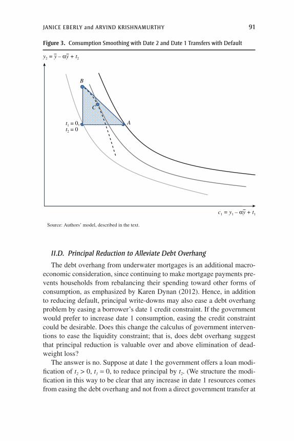
Suppose we solve the planning problem subject to the above budget con-straint and restrict attention to solutions where t1 and t2 are non-negative. Figure 3 illustrates the solution. The shaded area illustrates the set of all points such that t1 + t2 = Z, t1 > 0, and t2 > 0. It is clear that the solution is a corner: set t1 = Z and t2 = 0 (point A in the figure). This implies that principal reduction (in which t2 > 0) is not optimal, since the solution goes to the corner where the transfers are front-loaded, that is, for pay-ment reduction focused in period 1. This occurs despite the fact that our problem allows for strategic default with default costs and that borrowers default less if t2 > 0. For high enough Z, the transfer to date 1 is sufficient to ensure full consumption smoothing, and hence there is no need for further transfers.
In this setting, principal reduction is never optimal, even though default is costly and is accounted for by the planner, because the alternative of directly transferring the same resources to households in the first period raises utility more. It is optimal for the planner to use this strategy until the liquidity constraint no longer binds and consumption is completely smoothed. Until that occurs, principal reduction is suboptimal compared with payment deferral or reduction, and thereafter no policy intervention is needed to address liquidity constraints.
Janice eberly and arvind Krishnamurthy 91
II.D. Principal Reduction to Alleviate Debt Overhang
The debt overhang from underwater mortgages is an additional macro-economic consideration, since continuing to make mortgage payments pre-vents households from rebalancing their spending toward other forms of consumption, as emphasized by Karen Dynan (2012). Hence, in addition to reducing default, principal write-downs may also ease a debt overhang problem by easing a borrower’s date 1 credit constraint. If the government would prefer to increase date 1 consumption, easing the credit constraint could be desirable. Does this change the calculus of government interven-tions to ease the liquidity constraint; that is, does debt overhang suggest that principal reduction is valuable over and above elimination of dead-weight loss?
The answer is no. Suppose at date 1 the government offers a loan modi-fication of t2 > 0, t1 = 0, to reduce principal by t2. (We structure the modi-fication in this way to be clear that any increase in date 1 resources comes from easing the debt overhang and not from a direct government transfer at
Figure 3. consumption smoothing with date 2 and date 1 transfers with default
Source: Authors’ model, described in the text.
y2 = y – αy + t2
c1 = y1 – αy + t1
t1 = 0,t2 = 0
A
B
C

92 Brookings Papers on Economic Activity, Fall 2014
date 1.) Consider private lender transactions (t1, t2) that at least break even for the lenders, that is,7
(26) 1 0.2 2 1( )( )−τ − −τ − τ =F
In figure 3, we represent the principal reduction of Z by moving from the zero transfer allocation to point B. The dashed curve in figure 3 represents the set of trades, (t1, t2), that a private sector lender will make that allows the lender to break even. These trades allow agents to borrow against the future transfer Z in order to smooth consumption, solving the liquidity con-straint problem at date 1. Again, the critical thing to note is that the borrow-ing constraint becomes a curve. Starting from point B, the household will trade to point C, which achieves less utility than point A. That is, the house-hold will choose to borrow the Z back to increase date 1 consumption. However, since some borrowers default, the interest rate on the private loan will exceed 1, so that the government would do better by offering the transfer of Z at date 1, that is, a payment reduction rather than a principal reduction, to reach point A.
This is a general point: even if principal reduction is sufficiently gener-ous to overcome individual borrowing constraints, direct payouts to bor-rowers are more efficient since the government avoids the default costs associated with borrowing against home equity.8
The key insight underlying these results is the constraint affecting date 1 consumption. Even if credit markets exist to transfer date 2 resources into date 1 consumption, default risk makes this approach more expensive than a direct date 1 transfer to households. Hence, even with default risk, we again find that transfers in the initial crisis period at least weakly dominate policies that transfer resources later. Government resources to reduce prin-cipal are better spent in engaging lenders to renegotiate mortgage loans than in engaging them to write down loans directly.9
7. We assume that private lenders use the same discount rate as the government, even in the crisis. If the government can access credit markets at a lower rate than private lenders, our results are strengthened.
8. In general, principal reduction to reduce the underwater share of mortgages takes bor-rowers to an LTV (loan to value) of 100 at best, which does not generally create borrowing capacity. Even if it did, as we allow above, our analysis shows that direct transfers at date 1 remain more efficient.
9. Note that we have not assumed that the government has a lower cost of capital than private agents. This result relies only on the fact that by transferring resources at date 1, the government directly relaxes the liquidity constraint, whereas date 2 resources require the agent to borrow and transfer them to date 1. With any default risk, the price to agents of doing so will exceed the cost of the direct transfer.

Janice eberly and arvind Krishnamurthy 93
III. Optimal Date 1 Decisions and Default Timing
The economic environment during a crisis is explicitly dynamic, however, so borrowers, lenders, and policymakers have to decide not only what to do, but when to do it. These considerations can be quite important, since condi-tions may change unpredictably over time. Therefore, we now study the case where the borrower can take action at either date 1 or date 2, and informa-tion becomes available along the way. In the last section, we restricted the borrower to default only at date 2 in order to keep our analysis simple and establish the intuition for the default decision. Timing makes the problem more interesting and adds some potentially surprising results about delay.
The problem is somewhat more complex to study, but it does not change our conclusions on the benefits of payment reduction/deferral over prin-cipal reduction. Government resources spent on principal reduction for a borrower who remains current on his mortgage still has lower consump-tion benefits than a payment reduction that increases the borrower’s liquid-ity because of the liquidity constraint. Moreover, comparing equivalent payment and principal reductions, the payment reduction increases the borrower’s incentive to remain current on his mortgage and thus reduces default in addition to increasing consumption. This is again due to the liquidity constraint, whereby the borrower places a high value on continu-ing to service a mortgage that has been modified to reduce current pay-ments. Additionally, the analysis turns up a somewhat surprising result: borrowers who are underwater on a mortgage will typically continue to service it, because delaying the decision to default is a valuable option. Hence, borrowers need not be irrational or excessively optimistic when they continue to make payments on an underwater loan.
Suppose that at date 1 borrowers have information Ef ≡ Et=1[f] (that is, their mortgage at date 1 is underwater). Given this information, we ana-lyze the borrower’s decision at date 1, accounting for how the date 1 deci-sion affects the date 2 decision we analyzed in the previous section. If the borrower chooses not to default at date 1, then utility at date 1 is
( )α
+ − α
α−αy
ry t y(27) .1 1
1
If the household defaults at date 1, it can reoptimize its consumption plan to rebalance housing and nonhousing consumption, yielding a utility of
(28) 1 , where 1 .11
11( ) ( )( ) ( )α − α
= ψ ψ ≡ α − α
α−α
α−αy
ry
r

94 Brookings Papers on Economic Activity, Fall 2014
However, if the household defaults at date 1, it loses any value in the home as well as the option to delay default until date 2. Under default at date 1, date 2 wealth becomes y
_ - q, yielding a date 2 utility of
(29) .( )− θ ψy
With no default at date 1, utility at date 2 is
y E P t D[ ]{ }( )+ + − − θ ψ(30) max , .2 2
Hence, comparing values with and without a date 1 default, the default at date 1 occurs if
( )[ ]
( ) ( )
( )
ψ + − θ ψ > α + − α
+ + + − − θ ψ
α−α(31)
max , .
1 1 1
1
2 2
y yy
ry t y
E y P t D
Rewriting, we obtain the condition under which default occurs at date 1 as
( )[ ]−
+ − α
− α
> + φ
−α
y y
y t
yE t(32)
1max , 0 .1
1 1
1
2
Figure 4 graphs the left- and right-hand side of (32) as a function of Ef, which measures the degree to which a homeowner has equity (P2 - D) (plus the default cost), or the inverse of “underwaterness.” The gray curve graphs the value of the option to keep making mortgage payments and delaying default, on the right-hand side of equation 32. This value is uniformly posi-tive, although low for low values of Ef. The dashed line is the benefit of defaulting, on the left-hand side of equation 32. This value is independent of Ef. For low values of Ef, the household chooses to default at date 1.
The borrower chooses to default when the benefit of defaulting (the bold line) exceeds the benefit of delay (the gray line), given his level of equity and default cost. In option terms, underwater borrowers have a call option on keeping the home, which is extinguished by default. Thus the choice to make the mortgage payment at date 1 is not just about whether the loan is underwater; it is a question of whether the cost of making this payment covers the value of the call option. When liquidity constraints are tight, the cost of making the payment is highest; this determines the height of the horizontal bold line in Figure 4. When the borrower is underwater, the value of the call option is lowest, as shown in the gray line, which rises as
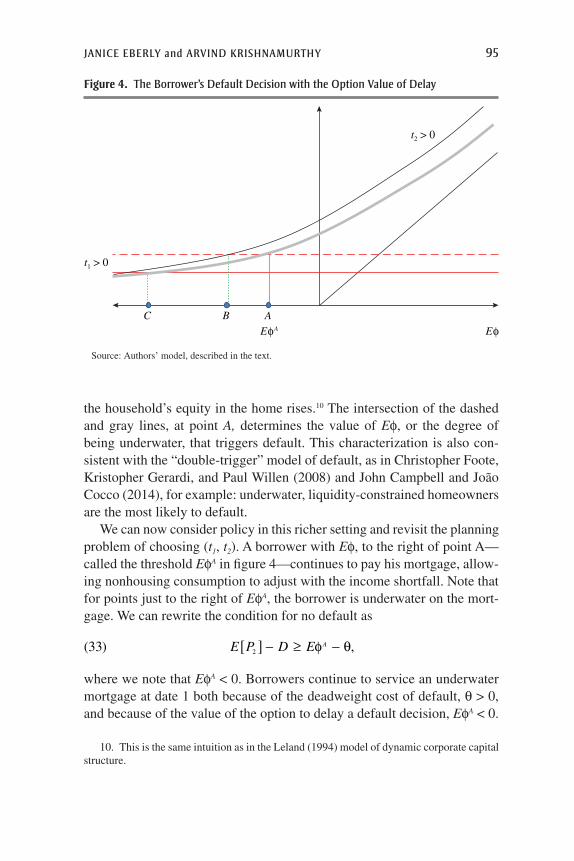
Janice eberly and arvind Krishnamurthy 95
the household’s equity in the home rises.10 The intersection of the dashed and gray lines, at point A, determines the value of Ef, or the degree of being underwater, that triggers default. This characterization is also con-sistent with the “double-trigger” model of default, as in Christopher Foote, Kristopher Gerardi, and Paul Willen (2008) and John Campbell and João Cocco (2014), for example: underwater, liquidity-constrained homeowners are the most likely to default.
We can now consider policy in this richer setting and revisit the planning problem of choosing (t1, t2). A borrower with Ef, to the right of point A—called the threshold EfA in figure 4—continues to pay his mortgage, allow-ing nonhousing consumption to adjust with the income shortfall. Note that for points just to the right of EfA, the borrower is underwater on the mort-gage. We can rewrite the condition for no default as
E P D E A[ ] − ≥ f − θ(33) ,2
where we note that EfA < 0. Borrowers continue to service an underwater mortgage at date 1 both because of the deadweight cost of default, θ > 0, and because of the value of the option to delay a default decision, EfA < 0.
10. This is the same intuition as in the Leland (1994) model of dynamic corporate capital structure.
Figure 4. the borrower’s default decision with the Option value of delay
Source: Authors’ model, described in the text.
t1 > 0
C B A
EφA Eφ
t2 > 0
96 Brookings Papers on Economic Activity, Fall 2014
For the underwater borrower who continues to service his mortgage, the problem is the same as we have analyzed in the previous section. The opti-mal transfer sets t1 > 0 and t2 < 0 to support date 1 consumption. However, when default is a possibility, the government may choose to set transfers and intervene to prevent defaults, avoiding foreclosure externalities and further deterioration in the housing market. We examine these effects and potential equilibrium feedback in more detail in the next section, but begin by examining the effect of transfers on defaults here.
Borrowers with Ef considerably below EfA will default independent of any transfers. Consequently, these are cases where the transfers gener-ate no economic benefits, so we set these cases aside. For borrowers with f near but just below EfA, transfers affect default incentives in interest-ing ways. Increasing t1 shifts down the benefit to defaulting (dashed line) at all values of Ef to the thin horizontal line. Hence the trigger value falls from point A to point C; the household will be more deeply under-water before defaulting. Increasing t2 increases the cost of defaulting, shifting up the solid gray curve to the dashed gray curve, and the trigger value falls from point A to point B. Note that this latter effect is stron-gest at higher values of Ef, on the right-hand side of figure 4. However, this is the region for which default is dominated; the default option is out of the money. Hence, positive date 2 transfers move equity values most when households are least likely to default. This point can be seen clearly analytically. The derivative of the left-hand side of equation 32 with respect to t1 is
y t
y−+ − α
− α
< −
−α
(34)
1
1.1 1
The derivative of the right-hand side of equation 32 with respect to t2 is
(35) 1.2
2
22
∫ ( )( )
∂ φ
∂= − <−
∞t dF
tF tt
Thus a dollar increase in t1 always decreases the benefit of defaulting at date 1 more than a dollar increase in t2. The difference in these effects increases as Ef falls, that is, as the mortgage is more underwater. Hence, the more underwater the loan is, the more effective an initial payment reduction is at avoiding default, relative to an equivalent transfer received

Janice eberly and arvind Krishnamurthy 97
at date 2.11 The date 1 transfer supports consumption and reduces default, reinforcing our finding that date 1 transfers are more effective than flat or back-loaded transfers. Initially, this was clear with a date 1 liquidity con-straint, but the same result obtains with date 2 default and now with the possibility of date 1 default and default timing on strategic default.
The option approach also illustrates the role of uncertainty, which raises the option value of waiting, or in terms of figure 4, shifts up the gray curve. The slanted straight line gives the payoff value under certainty (when f is known); greater uncertainty shifts the gray curve up relative to the slanted line. Higher home price uncertainty is therefore associated with fewer defaults at date 1, as homeowners have a greater option value of waiting for home prices to rise. This illustrates the subtlety of arguments about the effect of uncertainty on the economy. Putting a floor under home prices (reducing the mass in the left tail) would reduce defaults, but reducing uncertainty, or trading off a floor with a commensurate ceiling on home prices, could increase defaults.12
Finally, we note that a borrower who does not experience an income shock, y1 = y
_, never defaults at date 1. The left-hand side of equation 32
is zero in this case, because there is no benefit to reoptimizing date 1 con-sumption. Moreover, the right-hand side is strictly positive. Even in the case where c is expected to be negative, there is a positive value to wait-ing and exercising the option to strategically default at date 2, so that it is never optimal to default at date 1. This cleanly illustrates the intuition for strategic delay by unconstrained households.
We conclude from this analysis that payment reductions at date 1 are more effective than flat or back-loaded transfers in supporting consumption and preventing default at date 1. Principal reductions at date 2 are most
11. A mechanism such as this is apparent in the observed response of households to crisis-related cash transfers which, as documented by Hsu, Matsa, and Melzer (2014), had a significant effect in reducing foreclosures. They find that higher unemployment benefits (which are not repaid later) have a large impact in reducing the probability of default across states and over time.
12. The latter effect is likely to dominate in fact. Since the household defaults when the home price outlook is particularly bleak, the details of the left tail distribution do not mat-ter for behavior. That is, the details of bad outcomes do not matter to the household since it defaults in those states. However, the borrower does not default when home prices are expected to improve, so the upper tail is relevant for forward-looking decisionmaking. This is a generalization of Bernanke’s (1983) “bad news principle” in the two-sided setting of Abel, Dixit, Eberly, and Pindyck (1996). Here, we have a “good news principle” for borrow-ers because they have a default, or a put, option.

98 Brookings Papers on Economic Activity, Fall 2014
effective in preventing strategic default at date 2. This finding reinforces our earlier results for liquidity-constrained households. There, the bind-ing liquidity constraint made it clear that for macroeconomic consump-tion purposes, date 1 transfers are the most effective use of government budget resources. Allowing for future default modified this finding: date 1 payments coupled with repayment at date 2 can induce default at date 2. Hence, payments should be flatter but still front-loaded. A flat or back-loaded transfer schedule is always dominated by date 1 payments until the liquidity constraint is fully relaxed.13 With default and an option value of delay, we still obtain that policy transfers in the initial crisis period domi-nate policies that transfer resources later.
IV. Lender-Initiated Loan Modifications
We have shown that government resources aimed at supporting consump-tion and reducing default are better spent on payment reduction than on principal reduction. Because lenders directly bear the credit default risk, however, their incentives differ from the government’s. Unlike the gov-ernment, lenders may find it efficient to write down principal, because partially writing down principal may be cost effective compared to a default on the entire loan. We show that a lender’s incentives to do so are highest when the borrower is underwater on his mortgage and the strategic default risk is therefore highest. Moreover, as with the borrower, when the lender can time a principal write-down, the lender will choose to delay doing so until the time that a borrower is about to default on the mortgage loan.
IV.A. Date 2 Principal Reduction
We first consider the lender’s incentives at date 2 and then work back-ward to the dynamic problem at date 1. First consider a borrower whose home price exceeds the mortgage amount less the deadweight cost of
13. Our analysis assumes that the income shock is temporary, which is the interesting case for policy analysis to avoid default. If a shock is permanent but not common to all households, then default may be optimal as reallocation is necessary. In that case, optimal policy may still favor delay (if there is still price or other uncertainty to be resolved or the price elasticity of foreclosures declines over time). Government policy may also favor less-disruptive forms of default, such as short sales or rental-in-place arrangements, which can reduce the deadweight cost of default. Policy may also encourage lender renegotiation by giving more bargaining power to borrowers in these instances, through legal procedures such as bankruptcy and cramdown.

Janice eberly and arvind Krishnamurthy 99
default at the start of date 2. This borrower is expected to repay, and hence the lender receives the loan amount, D, plus the interest payment on the loan of rch. On the other hand, a borrower with f < 0 at the start of date 2 will be expected to default on his debt. In that case, the lender receives the home, which is worth P2, and which the lender can rent out to receive rch. Denote V2 (P2, D) as the value of the mortgage loan to a lender conditional on a given price P2 and debt level D. Then,
( ) =+ ≥ − θ
+ < − θ
V P DD rc P D
P rc P D
h
h(36) ,
if ;
if .2 2
2
2 2
Figure 5 graphs V2 (z) as a function of P2 for two levels of debt, D and D′ (where D′ < D). The comparison illustrates that when P2 < D - q (that is, f < 0), the lender can increase the value of its loan by reducing D to
Source: Authors’ model, described in the text.
V2(P2,D)
P2D – θ
D� – θ
D
D�
Figure 5. lender incentives for renegotiating loans to avoid strategic default
100 Brookings Papers on Economic Activity, Fall 2014
D′.14 This occurs because q is a deadweight cost of default. If the borrower defaults on his loan, the lender only collects P2. However, the borrower’s value of keeping the loan and not defaulting is P2 + q. Thus, the lender can offer to write down the principal to D′ < D and still increase the value of its loan.15 Formally, the lender renegotiation solves
( ) max , ,37 2 2′< ′( )D D V P D
with solution D′ = P2 + q for P2 < D - q.We have identified a situation where principal reduction leads to
better date 2 outcomes. Importantly, no government resources are required to implement the principal reduction, which is privately opti-mal since the lender benefits from avoiding default. As we point out later, though, the government may play an important role in encourag-ing and coordinating the renegotiation (for example, by standardizing the structure of modifications).
IV.B. Date 1 Principal Reduction
Now we move the lender’s valuation forward to consider a possible prin-cipal reduction at date 1, where lenders (and borrowers) observe Ef. If Ef is to the left of point A on figure 4, then borrowers will immediately default. In this case, the analysis of lender incentives is the same as just discussed. The lender will choose to immediately write down principal to P1 + q. Consider next the case where Ef is to the right of point A, but still below zero. In this case, borrowers will not default. Interestingly, lenders will also choose not to write down principal immediately. As in the previous section, this effect can be understood in terms of an American option, though here from the lender’s perspective. By waiting until t = 2 the lender can make the reduction
14. We assume that the lender has the bargaining power in renegotiation. In intermediate cases of shared bargaining power, the results would depend on the allocation of bargaining power, but the general findings would still hold. Furthermore, we have discussed the case when the borrower remains in his home. But as we showed in earlier sections, the loss of borrower wealth due to the decline in P2 will generally lead the borrower to consume less housing. Suppose the loan is renegotiated to D′, at which point the borrower immediately repays the loan by selling his home, and then rents a smaller home for one period. In this case, the lender’s payoff is D′ + rch, which is the same as in equation 36; thus our analysis is unaffected by this consideration.
15. In this analysis we are ignoring the fact that ex post loan forgiveness implies that lenders will thereafter expect loan forgiveness and price it into subsequent contracts, mak-ing credit more expensive. At this point, however, our intention is to examine under what circumstances even ex post loan forgiveness may make sense. We return to this topic later when we discuss ex ante security design.
Janice eberly and arvind Krishnamurthy 101
contingent on the realization of future prices, and specifically on whether or not P2 is below or above D - f. By writing down principal, the lender extin-guishes the option to write down later, and it is not optimal to exercise the option early. Formally, an early write-down has the lender maximizing:
( ) max , .38 2 2 1′< ′( )[ ]D D E V P D P
The lender loses value in doing so because maxD′<DE[V2(P2,D′)P1] < E[maxD′<DV2(P2,D′)P1], by Jensen’s inequality. This delay effect is rein-forced by any government transfer that decreases the incentive for default in figure 4, and hence reduces the incentive for a private lender renegotiation. Hence, a government write-down makes a private write-down less likely.16
In practice, there may be costs in waiting. It may take time to process the contractual requirements of reducing loan principal. Prices may move discretely and the borrower might default before the lender is able to imple-ment the reduction. Such considerations may lead the lender to reduce prin-cipal preemptively, although the value of delay will always be balanced against those considerations.
While it is inefficient for the government to write down principal, there may be circumstances where the government will prefer the lender to immediately write down principal. For example, a householder may be the best match for a home he is already living in and continue to ser-vice an underwater mortgage, restricting his nonhousing consumption and depressing economic activity in the crisis period. If the lender were to write down principal at date 1, the borrower would be less constrained and thus increase his nonhousing consumption at date 1, which may have macro-economic benefits. Our analysis shows that in order to incentivize lenders to write down principal early, the lender must receive a transfer equal to the value of the option to delay the write-down. That is, the government must “purchase” the option to delay the write-down from the lender in order to trigger an immediate write-down.
The cost of this option is E[maxD′<DV2(P2,D′)P1] - maxD′<D E[V2 (P2,D′)P1] > 0. In general, the value of this option will be less than the dollar amount of any principal write-down, so incentives for private write-downs may be effective even when the government does not write down the loan itself.
16. Moreover, we have not modeled the payment stream, but in practice, for loans not in distress, the lender continues to collect the interest and principal on the higher loan balance.

102 Brookings Papers on Economic Activity, Fall 2014
The last two sections of this paper demonstrate that delay can be desir-able to both borrowers and lenders, who see default as extinguishing a valu-able option to wait and possibly avoid costly foreclosure. The government may still intervene if it values the externalities associated with foreclosure or constrained consumption more than private agents do, and hence would prefer to move more quickly to address inefficient servicer delays, infor-mation problems, and capacity constraints. None of these actions involves principal reductions paid for by the government.17
V. An Adverse Selection Explanation for Lack of Modifications
In practice, lenders were not active in doing mortgage modifications, espe-cially during the early period in the financial crisis. Later, lenders began to offer principal reductions as part of loan modifications; this was especially true of specialty servicers. Lenders identified other considerations, includ-ing reputational effects and incentives affecting a lender’s whole portfolio of loans, rather than just individual borrowers. For loans not held on bal-ance sheet by lenders, servicer incentives and capacity may also have rein-forced delay and timing discreteness.
Our theoretical findings are consistent with the empirical work of Manuel Adelino, Kris Gerardi, and Paul Willen (2013), who document the reluctance of servicers to renegotiate mortgages and emphasize the presence of uncertainty arising from the risk of re-default and the “self-curing” of mortgage delinquencies. Other authors address administrative and structural frictions to loan renegotiation and recommend legal and policy changes to reduce them; for example, Christopher Mayer, Edward Morrison, and Tomasz Piskorski (2009) and John Geanakoplous and Susan Koniak (2011). The efficacy of these proposals is outside our pres-ent scope, although the challenges faced by servicers and the administra-tive structure of mortgages also point to the desirability of ex ante reforms (which we discuss in section VII) as opposed to ex post renegotiations.
In this section, we demonstrate one force arising naturally in our model that causes lenders to choose not to offer modifications. One disadvantage
17. We have kept the government and the lender separate for the sake of clarity. How-ever, in practice the government-sponsored enterprises (GSEs), Fannie Mae and Freddie Mac, are each a hybrid, where a government entity guarantees loans and hence holds credit risk. In this case, there is a direct incentive for these entities to write down principal as a way of avoiding costly defaults. In fact, there was an active debate around the extension of the PRA (principal reduction alternative) loan modification provision to the GSEs, which was ultimately not adopted by the GSE regulator, the Federal Housing Finance Agency (FHFA). The FHFA promoted an expanded refinance option, which we discuss later.
Janice eberly and arvind Krishnamurthy 103
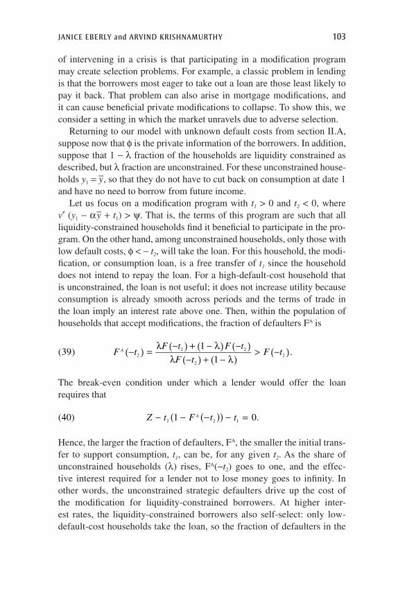
of intervening in a crisis is that participating in a modification program may create selection problems. For example, a classic problem in lending is that the borrowers most eager to take out a loan are those least likely to pay it back. That problem can also arise in mortgage modifications, and it can cause beneficial private modifications to collapse. To show this, we consider a setting in which the market unravels due to adverse selection.
Returning to our model with unknown default costs from section II.A, suppose now that f is the private information of the borrowers. In addition, suppose that 1 - l fraction of the households are liquidity constrained as described, but l fraction are unconstrained. For these unconstrained house-holds y1 = y
_, so that they do not have to cut back on consumption at date 1
and have no need to borrow from future income.Let us focus on a modification program with t1 > 0 and t2 < 0, where
v′ (y1 - ay_ + t1) > y. That is, the terms of this program are such that all
liquidity-constrained households find it beneficial to participate in the pro-gram. On the other hand, among unconstrained households, only those with low default costs, f < - t2, will take the loan. For this household, the modi-fication, or consumption loan, is a free transfer of t1 since the household does not intend to repay the loan. For a high-default-cost household that is unconstrained, the loan is not useful; it does not increase utility because consumption is already smooth across periods and the terms of trade in the loan imply an interest rate above one. Then, within the population of households that accept modifications, the fraction of defaulters FA is
( ) ( ) ( ) ( )( ) ( )
( )− = λ − + − λ −λ − + − λ
> −F tF t F t
F tF tA(39)
1
1.2
2 2
2
2
The break-even condition under which a lender would offer the loan requires that
(40) 1 0.2 2 1( )( )− − − − =Z t F t tA
Hence, the larger the fraction of defaulters, FA, the smaller the initial trans-fer to support consumption, t1, can be, for any given t2. As the share of unconstrained households (l) rises, FA(-t2) goes to one, and the effec-tive interest required for a lender not to lose money goes to infinity. In other words, the unconstrained strategic defaulters drive up the cost of the modification for liquidity-constrained borrowers. At higher inter-est rates, the liquidity-constrained borrowers also self-select: only low-default-cost households take the loan, so the fraction of defaulters in the

104 Brookings Papers on Economic Activity, Fall 2014
population goes toward one. For sufficiently high l, the modification mar-ket breaks down for standard “lemons market” reasons: the only contract offered is t1 = t2 = 0.
We can again write a planning problem to derive the optimal (t1, t2). The solution calls for t1 > 0 and t2 < 0, following the same logic as the previ-ous case. As l rises, there are more strategic defaulters in the pool, and the solution requires a smaller initial transfer t1.
Can the private market reproduce this outcome? Suppose that modifi-cations are offered by the private sector rather than by a government and that there is competition among lenders. Consider two lenders engaged in Bertrand competition. Fix a modification contract (t1, t2) such that the lend-ers each break even. Now suppose that one of the lenders offers a contract
t̂1 = t1 - e1 with = + �tt
ttˆ ˆ
22
1
1 2, for positive and small e1, e2.
The second contract involves a smaller date 1 loan, but also a smaller interest rate on the loan. The contract is not attractive to unconstrained borrowers because they will not repay, and hence care only about the size of the modification and not the effective interest rate. But we can always choose e1 and e2 such that the liquidity-constrained borrowers prefer the second contract over the first contract. That is, the interest-rate savings, e2, can be chosen to be large enough to compensate for the reduction in loan size, e1, to make this contract preferred by liquidity-constrained borrowers. In this case, the second contract is a profitable deviation by a lender. But as a result, the initial lender loses money, since this lender is left with a population of unconstrained strategic defaulters; he will therefore lose t1. The first lender will then have to match the second lender and reduce t1, but this offer will also be undercut. Equilibrium can unravel in the sense elaborated on by Michael Rothschild and Joseph Stiglitz (1976).
This logic provides two insights. First, it offers one reason why modifi-cations were not offered more widely. Competition and the fear of receiv-ing an adverse pool of borrowers likely limited lender modifications. Only in clear cases where the lender could exclude likely strategic defaulters through screens and filters could a modification proceed.18 Second, it offers a rationale for a standard government-supported modification contract.
18. A perverse example occurred early in the crisis, as pointed out by Mayer and others (2014), when the Countrywide modification program was made available to borrowers who defaulted by a future date, inducing strategic default leading up to the specified time. Such a design increased the cost of the program, whereas our model suggests program features to limit this adverse selection problem for modifications.

Janice eberly and arvind Krishnamurthy 105
That is, if the government supported and subsidized a standardized contract for all modifications, then the unraveling problem disappears.
VI. Housing Market Equilibrium and the Effect of Foreclosures
So far we have allowed uncertainty in home prices but not endogeneity. An additional reason to modify loans and reduce default might be to intervene in the dynamic equilibrium in the housing market from default to home prices and back to default, as documented empirically by John Harding, Eric Rosenblatt, and Vincent Yao (2008); John Campbell, Stefano Giglio, and Parag Pathak (2011); Atif Mian, Amir Sufi, and Francesco Trebbi (2011); and Anenberg and Kung (2014).
We are therefore interested in understanding how defaults and fore-closures at date 1 and date 2 affect housing prices. In this section we sketch a minimal general equilibrium of the housing market to clarify whether and how such considerations might alter our conclusions regard-ing modifications.
Denote pt as the price per unit of housing. Earlier, we described a house-hold purchasing ch
t units of housing services at price pt, so that the price per unit of housing was pt = Pt ⁄
=pP
ct
t
th. Equivalently, pt is the price of a normal-
ized quantity of a house of size “one.” Then,
[ ]= + +p E r r p(41) .0 1 2 2
Here r1 and r2 are the date 1 and date 2 user cost of housing, respectively. Next we close the model to specify a housing market equilibrium that determines p0. We follow our initial framework and assume that at a plan-ning stage, households anticipate income of y
_ at both dates and choose
housing consumption,
= αcy
rth
t
(42) .
At date 1, the household’s income falls to y1. For now, we assume that exogenously a fraction m1,L of the households default on their mortgages and enter the rental market, where L denotes the liquidity-constrained households. We can think of the households subject to the income shock and default as the liquidity-constrained households we modeled earlier.

106 Brookings Papers on Economic Activity, Fall 2014
We depart from our previous assumption and allow for a degree of fric-tion in the rental markets so that owning a home is more efficient than renting a home.19 To purchase one unit of housing services costs rt in debt service. The same housing services cost, if generated via the rental market, is frt, where f ≥ 1, and f parameterizes the rental friction, with f = 1 being the case we have analyzed in the previous section. Thus, the date 1 demand for housing via the rental market from the foreclosed homeowners is
= αcy
frh(43) .1
1
1
We assume that foreclosure keeps the household out of the ownership mar-ket for one period. At date 2, the household purchases a home again so that,
= αcy
rh(44) .2
2
Suppose that at date 1, across the economy there are ml,L agents renting, and 1 - ml,L agents owning. Then total demand for housing at date 1 from these agents is
( )α + − α = α − α −
(45) 1 .1
1 1 1
1,
1
1my
frm
y
r
y
rm
ry
y
fL
Foreclosures—that is, an increase in ml,L—decrease the net demand for housing at date 1. At date 2, since the date 1 foreclosed homeowners own
homes again, the total demand for housing is 2
α y
r and invariant to ml,L.
We assume that there are other unmodeled agents in the economy who also consume housing services. These may include new home buyers, home builders, speculators, and so on. We denote the demand from these agents as HD(rt). Our modeling only takes a stand on the functional forms for the households that are subject to foreclosure and that will be affected by modifications.
The market clearing condition at date 1 is
( ) + α − α −
=H r
y
rm
ry
y
fHD
L(46) ,1
1
1,
1
1
19. This may capture moral hazard or other information problems associated with the rental market.
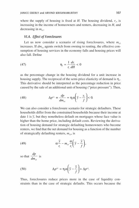
Janice eberly and arvind Krishnamurthy 107
where the supply of housing is fixed at H. The housing dividend, r1, is increasing in the income of homeowners and renters, decreasing in H, and decreasing in ml,L.
VI.A. Effect of Foreclosures
Let us now consider a scenario of rising foreclosures, where ml,L increases. If dml,L agents switch from owning to renting, the effective con-sumption of housing services in the economy falls and housing prices will also fall. Define
(47)1
01
1
1η = <r
dr
dH
as the percentage change in the housing dividend for a unit increase in housing supply. The reciprocal of the semi-price elasticity of demand is h1. This derivative should be interpreted as the percentage reduction in price caused by the sale of an additional unit of housing (“price pressure”). Then,
∆ ≡ = η α −
<p
dp
dmy
y
fL
L
(48) 0.1,
1,
11
We can also consider a foreclosure scenario for strategic defaulters. These households differ from the constrained households because their income at date 1 is y
_, but they nonetheless default on mortgages whose face value is
higher than the home price, including default costs. Reviewing the deriva-tion of housing demand for strategic defaulting homeowners who become renters, we find that the net demand for housing as a function of the number of strategically defaulting renters, ml,S, is
y
rm
ry
y
fSα − α −
(49) ,1
1,
1
so that 1,
dp
dm S
is
∆ = η α −
> ∆p y
y
fpS L(50) .1,
11,
Thus, foreclosures reduce prices more in the case of liquidity con-straints than in the case of strategic defaults. This occurs because the

108 Brookings Papers on Economic Activity, Fall 2014
liquidity-constrained defaulters experience a larger drop in the net demand for housing services when going from owning to renting. Note also that if f = 1, so that the rental market is frictionless, then Dp1,S = 0, and Dp1,L < 0.
We can repeat the same exercise at date 2. At date 2, all default is strate-gic. Thus, the effect of foreclosures at date 2 is
p yy
fS∆ = η α −
(51) .2,2
It is likely that the housing market is more stressed at date 1 in a recession than at date 2, so home sales have a bigger impact on price at date 1 than at date 2 and h1 > h2. In this case, it follows that we can order the effect of foreclosures on home prices as
∆ > ∆ > ∆(52) .1, 1, 2,p p pL S S
That is, the effect on home prices is largest from a default induced by liquidity constraint, which in our model occurs during the crisis period (date 1). Strategic defaults also put downward pressure on home prices, but less so, because these homeowners do not bring an income shock and payment distress into the rental market. Both of these effects ease once the economy moves out of the crisis period.
VI.B. Mortgage Modifications and Home Prices
We now revisit the question of how the proposed mortgage modifica-tions, parameterized by t1 and t2, would affect home prices. We showed earlier that payment reductions (that is, t1 > 0) are most efficient in reducing default at date 1, when households are liquidity constrained. Home prices are also most sensitive to defaults of liquidity-constrained agents. Putting these findings together, we conclude that if a planner’s objective includes home price stabilization (or if home prices feed back into consumption and utility), payment reductions for liquidity-constrained agents will be a more effective tool than principal reductions. Thus, payment reductions should be optimally targeted at liquidity-constrained agents. This finding reinforces our earlier conclusions on the benefits of payment reductions for liquidity-constrained agents.
Principal reductions (that is, t2 > 0) are less effective in reducing default at date 1, but they do help in reducing strategic default at date 2. Reducing

Janice eberly and arvind Krishnamurthy 109
strategic default at date 2 also stabilizes home prices, albeit less strongly than at date 1.
Consequently, endogenous home prices reinforce our general find-ing that policies that transfer resources to households during a crisis period at least weakly dominate policies providing transfers at later dates. Endogenous home prices also suggest that there is value in associat-ing these transfers with housing. That is, our earlier results, which focused on consumption smoothing alone, could have been accomplished with any type of transfer that supported consumption spending. With endogenous home prices, there is additional value to supporting spending on housing, specifically to prevent foreclosures and the negative effect they have on home prices.
VII. Ex Ante Security Design and the Automatic Stabilizer Contract
So far we have focused on policies put in place once a housing crisis is under way. We have considered only the effects of the policies at the time of implementation and not any effect on the cost of credit that might result from changing the terms of a loan after-the-fact. However, if loans are written down ex post, the cost of credit could rise as lenders anticipate and price in the probability of future write-downs. However, if these problems could be anticipated, policies could be put in place ex ante to ease the policy choices faced in the midst of a crisis.
To examine the security design that would result in our framework, we now shift back to a pre-crisis date 0 and examine the optimal state-contingent design of the mortgage loan. Using ex ante policies in principle avoids the moral hazard problems associated with ex post loan modifi-cations, and also avoids the pragmatic problems that would result from swiftly modifying potentially tens of millions of individual contracts in a crisis environment (as emphasized and documented in Agarwal and others 2011).
Our analysis of loan modifications has shown that different types of pol-icies solve distinct problems in the mortgage market: liquidity constraints and strategic default. The former is a cash-flow problem, whereas strategic default results from a high debt-to-value ratio giving the borrower a default incentive even when he is not in payment distress. A robust mortgage secu-rity should be able to address both of these issues.
From a security design perspective, the optimal security should elimi-nate the deadweight costs of default that are due to aggregate events, that is,

110 Brookings Papers on Economic Activity, Fall 2014
events not caused by the borrower. Moreover, the optimal contract should adjust payments in a state-contingent way to eliminate (or minimize) the incidence of the binding cash-flow constraint. Hence, liquidity constraints require that payments fall when the constraints tighten or become binding for more homeowners. Relaxing the liquidity constraints allows greater cash flow for nonhousing consumption and also reduces the probability of cash-flow-driven mortgage defaults. Therefore, this aspect of the optimal contract calls for a reduction in payments in states in which liquidity con-straints tighten.
The incentive for strategic default, on the other hand, calls for a dif-ferent policy prescription and in different states. In particular, in states in which the debt-to-value ratio rises, and especially when homeowners are underwater, the robust mortgage contract should reduce the amount of debt owed by the borrower. This reduces the incentive for strategic default and its associated deadweight costs. Indexing debt to macroeconomic outcomes has been proposed elsewhere, chiefly through indexing face value to home values (for example, Mian and Sufi 2014).
An optimal security design should consider these two objectives together. The optimal contract should both reduce payments in liquidity-constrained states and lower debt when the risk of strategic default rises. Put differ-ently, payments should fall during a recession, and debt should fall when home prices decline.
There is a simple contract, which we call an automatic stabilizer mort-gage contract, that goes some way toward implementing the optimal state contingency. This is a contract that allows the borrower the right to convert his fixed-rate mortgage to a floating-rate mortgage as long as he is not delinquent on his mortgage. Current mortgage contracts are priced to reflect the possibility that the borrower will prepay his mort-gage when market interest rates fall. From a pricing standpoint, prepay-ing a mortgage when market interest rates fall and converting it to one with a market floating rate have almost the same present value. How-ever, during the financial crisis, the prepayment option was curtailed for underwater loans, since they could not typically be refinanced (a new loan of equivalent amount was not available, since the loan exceeded the collateral value of the home). The main deviation from current prac-tice in our proposed contract is to remove this restriction and always give the borrower the option to convert his mortgage into a floating-rate mortgage.
The proposed contract achieves the two policy objectives: first, pay-ment relief, and second, principal reduction. It achieves the payment relief

Janice eberly and arvind Krishnamurthy 111
objective directly, since in a typical state of recession the central bank reduces short-term interest rates. Thus converting to a floating-rate mort-gage can substantially reduce current payments.
The second objective calls for a reduction in debt value when debt-to-value ratios rise, likely due to a decline in home prices. A reduction in debt value avoids the deadweight costs of default by strategic defaulters. In the abstract, allowing for this second objective requires a more complex contract, since the payment reduction and the loan write-down need not be coincident. However, as we argue next, resetting the mortgage interest rate can achieve the same loan value as a principal reduction and thus also achieve the second objective.
To see the parallels between reducing principal and lowering the mortgage interest rate, as in a refinancing, note that both methods of restructuring loans reduce the stream of payments on the mortgage over time. For a given fixed-rate, fixed-term loan, any new stream of payments that can be achieved with a reduction in face value can also be achieved by a reduction in the contract interest rate.20 This parallel between principal reduction and refinancing can be overlooked, because refinancing does not change the face value (principal) of the loan while principal write-downs explicitly reduce the face value. The distinction can be misleading, however, because face value is a poor measure of the value of a loan. On a market-value basis, resetting to a lower inter-est rate reduces the value of the loan. Mortgage lenders and investors see the effect in market valuations, and borrowers see the effect in their payments. A reduction in the payment stream achieved through a reduc-tion in face value can always be replicated by a change in the contract interest rate. For example—and to get a sense of magnitudes—a reset-ting of a 30-year $200,000 mortgage from a 6-percent interest rate to a 4-percent rate reduces monthly payments from $1,200 to $950 (20 per-cent), and the present value of the stream of payments from $250,000 to its face value of $200,000. The identical payment stream would result
20. While the present value of the payment streams can be equated, the time path differs. In particular, a written-down loan will have a lower initial payoff value, while a refinanced loan will have a lower payoff value than the original loan, but will amortize the remaining lower payoff value over time. The distinction does not affect the incentive for strategic default (since by definition the payoff value is not paid in case of default). However, it can matter for the incentive or ability to prepay the loan. Hence, face-value write-downs may tend to increase prepays and turnover more than refinancings do.

112 Brookings Papers on Economic Activity, Fall 2014
from a reduction in face value or principal write-down from $200,000 to $160,000 (or 20 percent).21,22
VII.A. Comments on Contracts and Modifications
We think of our proposed contract as a housing market version of auto-matic stabilizers, since it provides state-contingent support to both the housing market and the broader economy. This automatic stabilizer con-tract reduces payments when the economy is cyclically weak and liquidity constraints are likely to bind, and also reduces loan value when home prices fall. The cyclical movement of interest rates is key to the state contingency: If the central bank reduces rates during cyclical downturns and when home prices fall, the reset option allows mortgage borrowers to reduce their pay-ments and the present value of their debt. Various forms of home price insurance or indexation of contracts to home prices have been proposed (for example, Mian and Sufi 2014) to address the problems posed by neg-ative equity. If implemented at date 2, before default, these options also implement the intent to avoid strategic default at date 2. Some contracts of this type have been implemented on a small scale, although they have run into challenges with measuring home prices at the appropriate level of aggregation and allowing for home improvements and maintenance incen-tives. Indexing to interest rates, as suggested in the stabilizing contract, has the advantage of observability and consistency, preserving monetary policy effectiveness, and the fact that mortgage contracts with this feature already exist and are implemented and priced on a large scale.
21. Refinancings often further reduce payments by extending the term of the loan, but that would confound the effects of the interest-rate reduction and the term extension in this example, without changing the essential point.
22. Interestingly, refinancings generally occurred during the financial crisis in two ways. Either borrowers had positive equity and could refinance in a competitive market; these are unconstrained borrowers in our setting. This would have been possible regardless of the housing collapse. Alternatively, underwater borrowers from the GSEs, Fannie Mae and Freddie Mac, who were current on their loans, could refinance through the HARP program, and a similar option was made available to some non-GSE borrowers under the National Mortgage Servicing Settlement. (The terms of the National Mortgage Servicing Settlement are described here by the settlement monitor: https://www.jasmithmonitoring.com/omso/reports/final-crediting-report/) These borrowers were also arguably unconstrained, in that they were making their payments on time and were not in payment distress. Such circum-stances fit the model’s recommendation for implementing principal reduction for uncon-strained borrowers to avoid strategic default. (Because the program was made directly available to borrowers by the GSEs, lenders/investors did not have the option to delay.) Through HARP, borrowers received t1 > 0 and t2 > 0, financed by a reduction in the mortgage value held by lenders/investors.
Janice eberly and arvind Krishnamurthy 113
As discussed earlier, the parallels between principal reductions and mortgage rate reductions can be overlooked, perhaps because of the focus on face value in principal reductions. However, from the perspectives of both the lender and the borrower, the value or cost of a loan is the present value of payments, which may be equivalently reduced either by chang-ing face value or by changing the contract interest rate. For example, the Home Affordable Refinance Program (HARP), which allowed refinanc-ings of underwater GSE loans, is estimated to have completed 3.1 mil-lion HARP refinancings through the first quarter of 2014, out of a total of 19.2 million refinancings completed at the GSEs over the same period. The HARP refinancings include loans with LTV exceeding 80 percent, with about 12 percent of loans exceeding LTV of 125 percent. Interestingly, the GSEs started offering shorter-term (15- to 20-year) refinancing alterna-tives under HARP, and about 20 percent of underwater borrowers (with LTV greater than 105 percent) have shortened the loan term this way when refinancing. Consistent with our characterization of principal reduction for unconstrained underwater borrowers, this suggests that these borrowers are not liquidity constrained: by taking a shorter-term mortgage, they increased their mortgage payments when they could have chosen lower payments by extending the term of their new mortgages.23
To get a sense of magnitudes, the 30-year fixed-rate loan rate hit a trough in November 2012 at 3.35 percent (Freddie Mac PMMS, monthly average). Its peak in 2008 was 6.48 percent. If we use an average decline of 150 basis points due to refinancing on an average loan balance of $150,000, the pres-ent value of payments over the life of the loan falls by $28,000. The same payment reduction could have been achieved with a reduction in face value of 16 percent, or $24,000 for this typical loan. This method of achieving debt reduction relies on the sharp reduction in mortgage rates that occurred during the crisis. Empirical work has begun to examine the effectiveness of payment reduction through refinancing, including Fuster and Willen (2013) and Philip Bond and others (2014), who estimate that refinancing reduces the likelihood of mortgage default in the following year by one-third. Studies of other forms of cash transfers, such as that by Joanne Hsu, David Matsa, and Brian Melzer (2014), suggest that they can be effective in avoiding foreclosures. Separately, as emphasized by John Campbell in his presidential address to the American Finance Association (Campbell
23. FHFA Refinance Report (http://www.fhfa.gov/AboutUs/Reports/ReportDocuments/1Q2014RefinanceReport.pdf).

114 Brookings Papers on Economic Activity, Fall 2014
2006) and more recently by Benjamin Keys, Devin Pope, and Jaren Pope (2014), even households that are not underwater might fail to refinance when it appears to be available and desirable, so a mechanism to automate refinancing may have other social benefits.
Finally, while our model specified a date 1 reduction in income which then bounces back at date 2, the persistence of the recent housing crisis prompts examination of a case in which there is no recovery at date 2, so that the date 1 shock is permanent. “Date 1” in our model may encom-pass many years, and we have allowed date 2 income and prices to be uncertain. Nevertheless, the stabilizer contract we propose is robust in this dimension as well. A temporary shock requires temporary payment relief in order to avoid inefficient foreclosures and reductions in consumption; this payment relief occurs when a borrower refinances his loan. A per-manent shock—either a reduction in permanent income or a permanently lower level of home prices—requires a different policy. In this case, it is important whether the lasting shock is aggregate or idiosyncratic. If the persistent downturn is a common shock, then the optimal policy is one that keeps people in their homes. That is, even though home prices will fall, homes will not need to be reallocated. Indeed, foreclosures would only result in deadweight costs of foreclosure. In this case, payment relief and debt reduction reduce the incidence of foreclosure, so the stabilizer con-tract still has the relevant features.
On the other hand, if the date 1 shock is idiosyncratic and long lasting, then in equilibrium there should be turnover in housing and some real-location of homes will be required. That is, some homeowners will likely become renters, and vice versa. To the extent that reallocation is neces-sary, foreclosure is still inefficient because of its deadweight costs. In this case, the optimal policy should allow turnover while minimizing the dead-weight costs of foreclosure and encouraging efficient reallocation. Policy in this case could take the form of encouraging short sales and lender write-downs. In practice, modifications to keep borrowers in their homes during the crisis could also be useful for avoiding defaults while homeowners weather the crisis and learn about their ultimate economic prospects (for-mally, whether their shock is temporary or persistent).
VIII. Conclusions
The structure developed in this paper is very simple, as it is intended to pro-vide a conceptual framework for considering policy responses to a hous-ing crisis and recession. Its important features include liquidity constraints,

Janice eberly and arvind Krishnamurthy 115
reflecting households that cannot access housing equity or credit markets to smooth consumption, and the possibility of being underwater, reflecting households that not only have no home equity but may find it preferable to default on their mortgage, even when faced with the deadweight costs of default. In this setting, payment reduction during the crisis has favorable properties, both for supporting consumption during the crisis and hence achieving better macroeconomic outcomes and also for reducing default during the crisis.
Principal reduction can be helpful, but it is a less efficient use of gov-ernment resources, since it back-loads payments to households that cannot borrow against these future resources to support consumption today, and also because it is most helpful in reducing strategic default, rather than payment-distress-induced default. Defaults resulting from payment distress have a greater negative impact on home prices, since distressed borrowers carry their distress into the rental market and reduce housing demand more than defaults resulting from strategic considerations. When addressing stra-tegic default, lender incentives are aligned in the sense that lenders should renegotiate before default in order to avoid credit losses; the loan is worth more to the lender than is the collateral. Nonetheless, under uncertain con-ditions, it will be privately optimal for lenders to delay renegotiation as long as possible before default.
The government might have a different view from private agents, for various reasons. The government might value consumption and macro-economic performance more than individual agents do, and it might take foreclosure spillovers into account. These considerations should lead the government in two directions. First, the government should tend to provide more resources during the crisis period as a countercyclical measure—both to support consumption and to avoid defaults. Second, it should support lenders’ efforts at renegotiation, either by providing incentives or by pro-viding a standardized way of modifying and writing down loans to avoid strategic default and the associated deadweight costs, since private market efforts may be socially insufficient or may collapse entirely due to adverse selection.
Anticipating these ex post difficulties, an ex ante contract could incor-porate a stabilizing contract, through an expanded refinancing option. The standard prepayment option allowed for payment reductions as interest rates dropped substantially during the crisis. In particular, refinancing into a floating-rate ARM would allow for a much lower mortgage payment, easing the consumption constraint. However, when loans are underwater, prepayment is problematic, since borrowers cannot finance the underwater

116 Brookings Papers on Economic Activity, Fall 2014
portion of the loan. We therefore propose a reset option to allow a mortgage to be converted into an ARM even when the loan is underwater. Such a contract would implement the optimal contract and fill the role of auto-matic stabilizers in the housing market. This stabilizing contract would allow a state-contingent modification to reduce payments and would solve the debt write-down problem under those conditions when interest rates fall coincidentally with a drop in home prices.
Our proposed mortgage contract limits consideration to existing policies around housing, and in particular, around mortgages. Other forms of fiscal and monetary policy may be useful in our setting; indeed, the fact that our proposed mortgage contract is indexed to interest rates suggests that mon-etary policy is powerful in this setting. Similarly, fiscal policy to transfer resources to date 1 and alleviate the liquidity constraint would be effective, and perhaps more so than a housing payment reduction.
However, we focus on housing by design, because we are addressing the implications of a housing crisis, which includes falling home prices. In particular, policies to reduce mortgage default may have outsized effects in a housing crisis, so focusing resources on mortgage borrowers may be unusually relevant. Moreover, targeting homeowners may be an especially effective way of reaching liquidity-constrained households during a hous-ing crisis. This does imply that it is universally more effective than trans-fers or tax policy to increase liquidity more generally in the crisis period, but as we show, mortgage policies can alleviate the distress induced by a home price collapse.
Finally, we have intended this paper to provide a framework for con-sidering various types of credit policy in a simple setting. As credit policy becomes a common component of both fiscal and monetary policy, such a framework may be useful more broadly. For example, empirical questions have arisen around the use of credit policy to finance human capital acqui-sition (such as student loans) as well as housing (through the GSEs and FHA), where such a framework could be a valuable tool.
ACknOwLEDgMEnTS We benefited from the helpful comments of Andy Abel, Gene Amromin, Philip Bond, Zhiguo He, and our discus-sants, Austan Goolsbee and Paul Willen, as well as research assistance from Ryan Shyu. We have no relevant material or financial interests to declare regarding the content of this paper.
Janice eberly and arvind Krishnamurthy 117
References
Abel, Andrew, Avinash Dixit, Janice Eberly, and Robert Pindyck. 1996. “Options, the Value of Capital, and Investment.” Quarterly Journal of Economics, August: pp. 753–7.
Adelino, Manuel, Kris Gerardi, and Paul Willen. 2013. “Why Don’t Lenders Rene-gotiate More Home Mortgages? Redefaults, Self-Cures and Securitizations.” Journal of Monetary Economics 60, no. 7: 835–53.
Agarwal, Sumit, Gene Amromin, Itzhak Ben-David, Souphala Chomsisengphet, and Douglas D. Evanoff. 2011. “Market-Based Loss Mitigation Practices for Troubled Mortgages Following the Financial Crisis.” Working Paper. Federal Reserve Bank of Chicago.
Anenberg, Elliot, and Edward Kung. “Estimates of the Size and Source of Price Declines due to Nearby Foreclosures.” Working Paper no. 2012-84. Federal Reserve Board of Governors (and forthcoming, American Economic Review).
Bernanke, Ben S. 1983. “Irreversibility, Uncertainty, and Cyclical Investment.” Quarterly Journal of Economics 97, no. 1: 85–106.
Bond, Philip, Ronel Elul, Sharon Garyn-Tal, and David Musto. 2014. “Does Junior Inherit? Refinancing and the Blocking Power of Second Mortgages.” Working Paper. University of Washington.
Campbell, John Y. 2006. “Household Finance.” Presidential address made before the American Finance Association. Journal of Finance 61, no. 4: 1553–1604.
Campbell, John Y, and João F. Cocco. 2014. “A Model of Mortgage Default.” (February 2014 version). Harvard University.
Campbell, John Y., Stefano Giglio, and Parag Pathak. 2011. “Forced Sales and House Prices.” American Economic Review 101, no. 5: 2108–31.
Dynan, Karen. 2012. “Is a Household Debt Overhang Holding Back Consump-tion?” Brookings Papers on Economic Activity, Spring: 299–334.
Eggertson, Gauti, and Paul Krugman. 2010. “Debt, Deleveraging, and the Liquid-ity Trap: A Fisher-Minsky-Koo Approach.” Working Paper. Federal Reserve Bank of New York.
Farhi, Emmanuel, and Ivan Werning. 2013. “A Theory of Macroprudential Policies in the Presence of Nominal Rigidities.” Working Paper no. 19313. Cambridge, Mass.: National Bureau of Economic Research.
Federal Housing Finance Agency (FHFA). 2014. “Refinance Report—First Quarter 2014.” http://www.fhfa.gov/AboutUs/Reports/ReportDocuments/1Q2014RefinanceReport.pdf
Foote, Christopher, Kristopher Gerardi, and Paul S. Willen. 2008. “Negative Equity and Foreclosure: Theory and Evidence.” Journal of Urban Economics 64, no. 2: 234–45.
Fuster, Andreas, and Paul Willen. 2012. “Payment Size, Negative Equity, and Mortgage Default.” Public Policy Discussion Paper no. 12-10. Federal Reserve Bank of Boston.

118 Brookings Papers on Economic Activity, Fall 2014
Geanakoplous, John, and Susan Koniak. Undated. “Why the Blind Trustee Plan is Cheaper and Better than Alternatives.” Working Paper. Yale University. http://www.law.yale.edu/documents/pdf/cbl/Koniak_Blind_Trustee.pdf
Guerrieri, Veronica, and Guido Lorenzoni. 2011. “Credit Crises, Precautionary Savings, and the Liquidity Trap.” Working Paper No. 17583. Cambridge, Mass.: National Bureau of Economic Research.
Hall, Robert. 2011. “The Long Slump.” American Economic Review 101, no. 2: 431–69. https://ideas.repec.org/a/aea/aecrev/v101y2011i2p431-69.html
Harding, John P., Eric Rosenblatt, and Vincent Yao. 2008. “The Contagion Effect of Foreclosed Properties.” Journal of Urban Economics 66, no. 3: 164–78.
Howard, Greg, Robert Martin, and Beth Anne Wilson. 2011. “Are Recoveries from Banking and Financial Crises Really So Different?” International Finance Discussion Paper no. 1037. Washington: Board of Governors of the Federal Reserve System.
Hsu, Joanne, David Matsa, and Brian Melzer. 2014. “Positive Externalities of Social Insurance: Unemployment Insurance and Consumer Credit.” Working Paper no. 20353. Cambridge, Mass.: National Bureau of Economic Research.
International Monetary Fund. 2012. “Dealing with Household Debt.” Chapter 3 in World Economic Outlook (April). Washington.
Keys, Benjamin, Devin Pope, and Jaren Pope. 2014. “Failure to Refinance.” Work-ing Paper no. 20401. Cambridge, Mass.: National Bureau of Economic Research.
Leland, Hayne. 1994. “Corporate Debt Value, Bond Covenants, and Optimal Capi-tal Structure.” Journal of Finance 49, no. 4: 1213–52.
Mayer, Christopher, Edward Morrison, and Tomasz Piskorski. 2009. “A New Pro-posal for Loan Modifications.” Yale Journal on Regulation 26, no. 2: 417–29.
Mayer, Christopher, Edward Morrison, Tomasz Piskorski, and Arpit Gupta. 2014. “Mortgage Modification and Strategic Behavior: Evidence from a Legal Settle-ment with Countrywide.” American Economic Review 104, no. 9: 2830–57.
Mian, Atif, and Amir Sufi. 2009. “The Consequences of Mortgage Credit Expan-sion: Evidence from the U.S. Mortgage Default Crisis.” Quarterly Journal of Economics 124, no. 4: 1449–96.
———. 2014. House of Debt. University of Chicago Press.Mian, Atif, Amir Sufi, and Francesco Trebbi. 2011. “Foreclosures, Home Prices,
and the Real Economy.” Working Paper no. 16685. Cambridge, Mass.: National Bureau of Economic Research.
Reinhart, Carmen, and Kenneth Rogoff. 2009. “The Aftermath of the Financial Crisis.” American Economic Review 99, no. 2: 466–72. https://www.aeaweb.org/articles.php?doi=10.1257/aer.99.2.466
Rothschild, Michael, and Joseph Stiglitz. 1976. “Equilibrium in Competitive Insur-ance Markets: An Essay on the Economics of Imperfect Information.” Quarterly Journal of Economics 90, no. 4: 629–49.
119
Comments and Discussion
Comment ByAUStAn GooLSBee In the aftermath of the housing and financial crisis, there has been considerable debate and second guessing about a great many things and especially about housing policy. One of the most contro-versial of those debates has centered on the idea of principal reduction and whether the government’s response to the crisis should have included more explicit efforts to write down mortgage debt for consumers.
Some of the advocates of that view come from a perspective of fairness— that the benefits of the bank bailouts were concentrated in the banks them-selves and not shared with ordinary homeowners. Others view it as an economic positive, arguing that only reducing the amount of outstanding debt would have allowed the consumer balance sheet to improve sufficiently to induce consumers to begin spending again the way they did before the crisis. By implication, this also argues that the recession has been longer because of the lack of principal reduction.
Most of the arguments about which approach is better, and even about which housing goal we should be targeting, have had only a vague theoreti-cal basis. This paper by Jan Eberly and Arvind Krishnamurthy attempts to rectify that by producing a straightforward, simplified model of optimizing consumers who receive a negative shock and attempt to rebalance their consumption. Their model is able to confront and inform a surprisingly rich set of economic phenomena and behavior. It is enough to make one wish that all public commentators on the topic would be required to write down the model that underlies their own arguments.
From their model, Eberly and Krishnamurthy show several important things. First, when one is faced with a borrower liquidity crisis, mortgage modifications that reduce monthly payments are more effective at helping consumers rebalance their consumption, in a bang-for-the-buck sense,

120 Brookings Papers on Economic Activity, Fall 2014
than writing down mortgage principal of the same magnitude. Second, the benefits of principal reduction come from reducing the incentives for strategic defaults, so that even though government policies to support rebalancing consumption are better off modifying payments, the mort-gage lenders themselves will have an incentive to reduce mortgage prin-cipal to prevent default. Third, in the world described by their model a new type of mortgage becomes quite appealing: basically, it is a one-way ARM—automatically lowering mortgage rates (and thus monthly payments and total debt loads) when rates fall.
I was heavily involved in the housing policy discussion during the 2008–11 period, at least on the White House’s side, and I admit that this involvement colors my reaction to the paper’s findings. I believe the direct experiences attempting to provide housing relief shed some light on which parts of the theoretical model are most useful and which could use some further examination.
Why There Wasn’T Much PrinciPal reducTion in u.s. housing Policy.
The essence of the housing policy problem in 2009 was that the data suggested that about 25 percent of homeowners were underwater, and the amount of negative equity among those homeowners was on the order of $700–$800 billion (First American CoreLogic 2012; Hubbard and Mayer 2009). These underwater homes were forecast to translate into 8–10 million impending foreclosures, although people debated whether it was to be strategic default or traumatic default that would cause them.
The basic question for policy was very much the question posed in this paper: What is the best thing to do with the limited government resources? The government did not have an additional $800 billion to pay off people’s mortgages (and even if it had, it would have had to deal with a major politi-cal outcry about rewarding the undeserving who had borrowed beyond their means). The banks, grappling with issues of insolvency, could not recognize an additional $800 billion in losses on their balance sheets. Con-sumers seemed unlikely to be able to repay the $800 billion themselves in a troubled economy. There would, in the end, be a much smaller amount of government money made available, a subset of the Troubled Asset Relief Program (TARP), that could be used to help fight foreclosures, and the argument centered on the best way to do so.
Some influential economists have argued that we needed principal reduc-tion (including Geanakoplos and Koniak 2009, Stiglitz 2010, Shiller 2012, Mian and Sufi 2014). But in his review of Atif Mian and Amir Sufi (2014), Larry Summers (2014) notes that with a marginal propensity to consume out of housing wealth of about 15 percent, the impact on short-run consumption

coMMenTs and discussion 121
and output of principal reduction would have been modest compared to other forms of stimulus. That view is fully in keeping with the thinking of Eberly and Krishnamurthy here. With something like $25 billion to spend on housing relief, reducing negative equity by less than 3 percent of the total did not seem like a particularly efficient way to reduce foreclosures or help the economy.
The other problem with principal reduction—one that fits rather less comfortably with the current paper’s view that the lenders have strong incen-tives to reduce on their own—was the basic fact that banks and mortgage holders refused to write down principal. Some argued that the government should either force them to do so as a condition of receiving bailout money or else allow judges to impose cramdowns of mortgages in bankruptcy (in most bankruptcies home mortgages remain exempt from restructuring). In reality, the TARP money had already gone out to the banks before the Obama administration came into office, so there was not much wiggle room to attach conditions on it after the fact. And concerning bankruptcy cramdown—Congress made it quite clear it would prevent that.
The federal government had actually tried a major policy to encourage write-downs earlier, and it formed the backdrop of all the housing policy discussions in 2009. The 2008 Hope for Homeowners program had sought to encourage lenders to write down principal on underwater mortgages by offering the mortgage holders a government guarantee on the new, smaller, over-water mortgage. This policy failed completely. The Congressional Budget Office had estimated that the policy would help 400,000 home-owners. The actual number of homeowners helped, as reported by the Federal Housing Administration in 2011, was 762 (FHA 2011).
Why would lenders not write down principal, if as the theory predicts it would be in their own interest to do so in order to prevent strategic default?
One reason is that American homeowners proved to be almost patho-logically honest. Default rates were then, and remain today, well below the share of people underwater. Even among people very heavily underwater, the large majority continued making their payments. Banks decided that it did not make sense to give write-downs to people that would keep paying anyway. Basically, the amount of strategic default seemed notably low, so the lenders were, perhaps, not so concerned with the importance of reducing its incidence.
Beyond that, the majority of the mortgages that might benefit from a write-down had been securitized, so the writing down of principal ignited all sorts of so-called “tranche warfare.” Without a single owner, the mortgage-

122 Brookings Papers on Economic Activity, Fall 2014
backed securities (MBS) investors were often at odds over what they wanted for the mortgages embodied in their securities. Buyers of an AAA rated tranche might have an incentive for the properties to foreclose, while owners of a low-priority BB tranche might strongly prefer a modification that could avoid default. Often the ownership was so diffused that the owners could not be reached at all.
Why Policy Turned To MorTgage ModiFicaTion and The iMPleMenTaTion
issues ThaT FolloWed. In sum, principal write-down seemed to be a non-starter in practice, or at least an extraordinarily expensive and hard-to-get-started option. Instead, the White House opted for a mortgage modification program that would subsidize a cut in the interest rate of the borrower with-out reducing the principal in an effort to get the monthly payment down to 31 percent of income (our “affordability” threshold) as part of the Home Affordable Modification Program (HAMP).
The rationale was fairly simple. The owner-occupier of a house values it more than anyone else in the market does because of the costs of moving, of changing schools, and so on. A policy of affordability-modification-without-principal-reduction could therefore exploit a wedge. It could get people to stay in houses that were underwater using less money than would be necessary to buy down their principal directly. Eberly and Krishnamurthy also add the option-value insight that homeowners may stay in their negative-equity homes just to keep their option open that their home values might go back up in the future.
Essentially, the theoretical model in this paper argues that this modi-fication approach is the most efficient way to help homeowners in a liquidity crisis. The model concentrates the relief in the current period instead of spreading the relief out over the life of the mortgage as would happen in a principal reduction plan. I find the logic persuasive. I would add that the later empirical work of Andreas Fuster and Paul Willen (2013) rather clearly documents that the idea of the paper is spot-on, since they find that even among people who are underwater, once their payments fell to a level they could handle they stayed in their houses and kept paying.
There were some practical problems with implementing HAMP’s theoretically sound policy of modification, however, problems that anyone should ruminate on before proposing radical changes to housing finance.
For example, lenders agreed to participate in the HAMP modifications and agreed to give trial modifications to anyone whose stated income would qualify them for the program until their documentation came through

coMMenTs and discussion 123
(tax return records, pay stubs, and so on). If they did not qualify at that point, they would not continue with the lower payment modification, but it gave a free option to consumers. But some banks themselves lacked inter-nal controls, so that even as one side of the bank gave a reduced payment modification, a different part of the bank counted the lower payment as delinquency and commenced foreclosure proceedings on the homeowner. This was called the “dual-tracking problem.” Often the homeowners sued, successfully, to get the houses back, but they won only after a lengthy delay, during which the houses became dilapidated or were ransacked for materials by thieves while they lay dormant. It was an absurd problem, one that did not make theoretical sense, and yet there were thousands of people dealing with it in reality.
Many mortgage servicers lacked the capacity to process modifications at all. This meant that the benefits of mortgage modification to the borrower depended heavily on who happened to have the service contract for their securitized mortgage (a matter that the borrower had very little control over).
On the borrowers’ side, many people were afraid of being thrown out of their houses, and having endured collection agencies calling them to get money were trying to avoid any contact with the lenders. This fear extended even to cases where lenders were actually offering them beneficial subsidized modifications that would reduce their payments by thousands of dollars a year at no cost to them. Large numbers of people simply would not respond.
The government also tried to institute an “automatic” refinancing for underwater mortgages backed by the GSEs that had over-market interest rates but could not refinance because the loan-to-value ratios were too high. The government already had the credit risk in these cases. But the market for GSE bonds included attestations that loan-to-value ratios not exceed various cut-offs, which meant that every house required an appraisal and new title insurance, gumming up any chance of defaulting the mortgages into lower rates.
These kinds of impediments to refinancing are largely what motivates Eberly and Krishnamurthy to say that designing a mortgage that could adjust downward without having to get tranche approvals, re-appraisals, and title insurance would be a big improvement in their model. It is easy to see why that is true, but their model is not subtle enough to say anything about the importance of liquidity in housing finance markets. If their proposed new mortgages had only modest take-up, the experience of the crisis makes me think that liquidity for these instruments would be very low and their prices would be too high to get them on a path to wider adoption.

124 Brookings Papers on Economic Activity, Fall 2014
is This The righT Kind oF Model To undersTand a housing BuBBle? As productive as it can be to apply a model like this to comparing different housing policies, one ought to have a nagging fear in the back of one’s mind when doing so. The essence of the model is a rational equilibrium—namely, consumers are maximizing consumption in period one, something bad happens, and they try to smooth consumption in period two as best they can. In the housing boom of the 2000s, however, there were millions of people buying homes that were completely out of their league. They qualified for mortgages they had no business taking, which implied a level of housing consumption that could not be sustained. One can debate the question of why rational lenders were willing to make those loans (because of agency problems with the loan originators? mistaken beliefs that house prices could never decline? government encouragement?) and likewise why consumers would want to take them (because people figured the banks would know what consumers could afford? mistaken beliefs that prices could never decline? speculative frenzy?). But lenders made them, and people took them.
So, does it make sense to ask in these cases about rebalancing optimal consumption in response to an income shock? The consumption levels in period one were completely out of equilibrium. The country was in the middle of a bubble. The premise of this model and also of advocates of principal reduction (like Mian and Sufi) is figuring out how to restore con-sumption in the quickest way possible. But perhaps we should ask whether policy really ought to try to restore consumption to levels that made no sense to begin with. To me, that seems like a question worth answering for anyone looking at how we should direct our housing policy.
reFerences To The goolsBee coMMenT
Federal Housing Administration (FHA). 2011. “Annual Management Report Fiscal Year 2011.” http://portal.hud.gov/hudportal/documents/huddoc?id=fhafy11annual mgmntrpt.pdf
First American CoreLogic. 2012. “Negative Equity Q1 2012.” August. http://www.corelogic.com/downloadable-docs/negative_equity_q1_2012.pdf
Fuster, Andreas, and Paul Willen. 2013. “Payment Size, Negative Equity and Mortgage Default.” Staff Report no. 582. Federal Reserve Bank of New York.
Geanakoplos, J., and S. Koniak. 2009. “Matters of Principal,” New York Times, March 4.
Hubbard, R. Glenn, and Christopher J. Mayer. 2009. “The Mortgage Market Meltdown and House Prices.” B.E. Journal of Economic Analysis & Policy 9, no. 3: 1–47, March.

coMMenTs and discussion 125
Mian, Atif, and Amir Sufi. 2014. House of Debt: How They (and You) Caused the Great Recession, and How We Can Prevent It from Happening Again. Chicago: University of Chicago Press.
Shiller, R. 2012. “Reviving Real Estate Requires Collective Action.” New York Times, June 23.
Stiglitz, J. 2010. “Foreclosures and Banks’ Debt to Society.” The Guardian, November 5, 2010.
Summers, L. 2014. “Lawrence Summers on ‘House of Debt’: Did the response to the financial crisis focus too much on banks while neglecting over-indebted homeowners?” Financial Times, June 6.
Comment ByPAUL WILLen In this paper, Janice Eberly and Arvind Krishnamurthy use a model of an optimizing household to evaluate the claim that compul-sory principal reduction was the optimal policy response to the problem of underwater homeowners during the Great Recession. They show that in an economy populated by borrowing-constrained households, principal reduc-tion is rarely the most cost-effective form of relief for borrowers. Reducing the size of monthly payments is a better idea.
To grasp the logic of the model, consider first the claim that reducing principal stimulates consumption. A household facing a binding borrow-ing constraint has a marginal propensity to consume (MPC) of 1 out of a reduction in the current monthly payment. On the other hand, constrained households have an MPC of 0 out of a reduction in future payments because their consumption is already limited by the constraint. Principal reduction differs from payment reduction solely in its effect on future payments, so it is easy to see that a dollar spent on principal reduction should have a much smaller effect than a dollar spent on payment reduction.
The logic of Eberly and Krishnamurthy was, implicitly, recognized by policymakers during the crisis. My table 1 shows estimates by Mark Zandi of Moody’s of the marginal propensity to consume used in a calculation of the effects of the American Recovery and Reinvestment Act of 2009. Zandi assumes that lower-income households are borrowing constrained and thus will consume most of a temporary increase in after-tax income. Even higher-income households will consume a relatively large fraction.
How does principal reduction match up to other forms of stimulus? If we use the estimates of Atif Mian and Amir Sufi, two of the most out-spoken advocates of principal reduction, heavily indebted households would

126 Brookings Papers on Economic Activity, Fall 2014
have spent 18 cents of every dollar of principal reduction they received.1 The MPC used by Mark Zandi (2010) for the households with the lowest MPC is twice as large as the MPC claimed by Mian and Sufi for the group with the highest MPC out of principal reduction. If Congress had wanted to spend one more dollar on stimulus in 2009, it is clear that principal reduc-tion would have come at the bottom of the list.2
Now consider the second ostensible effect of principal reductions: reducing foreclosures. For this analysis, the Eberly-Krishnamurthy model marries the logic of borrowing constraints to a modern conception of the mortgage default decision. The borrower decides whether to default each month when his monthly payment is due. By defaulting, the borrower can free up money for extra consumption and reduce his future liabilities, but he also forfeits any future price gains that accrue to the house. For a constrained household, the marginal value of consumption today is far higher than both the marginal value of consumption in the future and the riskless interest rate. Consequently, reducing current payments and raising current consumption has a disproportionately strong effect on the default decision. Here again, the data confirm the theory. Andreas Fuster and Paul Willen (2013) show that the effect of a 50-percent temporary reduction in mortgage
Table 1. effect of infrastructure and Tax cuts on Marginal Propensity to spend
Infrastructure $1
Tax cuts (by income quintile) 1 $1.12 2 $0.70 3–4 $0.44 5 $0.40
MDR $0.05–0.07“Targeted MDR” $0.18
Source: Zandi 2010.
1. Atif Mian and Amir Sufi, “Why Tim Geithner Is Wrong on Homeowner Debt Relief,” Wonkblog (blog), Washington Post, May 14, 2014. http://www.washingtonpost.com/blogs/wonkblog/wp/2014/05/14/why-tim-geithner-is-wrong-on-homeowner-debt-relief/
2. Mass principal reduction would have required taxpayer funds. According to the Flow of Funds, more than half the mortgage debt outstanding in 2009 was directly insured by the federal government and a majority of the rest was held on the balance sheets of depository institutions insured by the federal government. Mortgage-backed securities not insured by the government accounted for less than 20 percent of mortgage debt.
coMMenTs and discussion 127
payments for a household with a loan-to-value ratio of 135 is equivalent to a reduction in loan-to-value of 35 percent.
All in all, the model of Eberly-Krishnamurthy confirms the likely intuition of many policymakers during the housing crisis. Payment reduction front-loads relief in the current period, whereas principal reduction spreads it out over the life of the loan. As a result, payment reductions are likely to be particularly effective both as stimulus and as anti-foreclosure policy if borrowers are liquidity constrained. An important advantage of the Eberly-Krishnamurthy model is that it can be used to lay out ideal policies that take this logic into account.
How closely did the policies that were actually enacted compare to the idealized polices from the model? In the wake of the crisis, three things happened. First, lenders foreclosed on millions of homeowners. Fore-closure is not a pleasant experience but, for most borrowers, it results in the complete elimination of their mortgage obligations.3 In other words, it is a dramatic form of principal reduction. Second, policymakers made a concerted effort to drive down mortgage interest rates. The Federal Reserve lowered short-term interest rates to zero and then purchased trillions of dollars in various financial assets in hopes of lowering long-term rates further.4 Economists will debate the quantitative impact of large-scale asset purchases for years, but in the third quarter of 2008, the Freddie Mac Primary Mortgage Market averaged 6.52 percent. In the first quarter of 2009, it averaged 5.16 percent, and by the end of 2012 the average had fallen to 3.36 percent.
To be sure, many borrowers had trouble refinancing, but many did not. My figure 1 shows how powerful the inducements to refinancing were. By the end of 2010, about half the debt outstanding before the crisis had been retired, either by foreclosure or by refinancing into a lower interest rate. The figure shows that this reduction was true for a sample of all loans as well as for a sample of the riskiest loans, that is, loans sold in private-label securities. Indeed, in one of the hardest-hit states, Nevada, only one-third of pre-crisis debt remained outstanding at the end of 2010.
3. Lenders can pursue borrowers for the “deficiency,” the difference between what the borrower owes and what the lender recovered from the foreclosure, but they rarely do. FHFA data suggest a recovery rate of less than 1/4 percent (see FHFA, Office of the Inspector General 2012).
4. In particular, between 2008 and 2014 the Federal Reserve purchased $2.8 trillion of agency MBS.
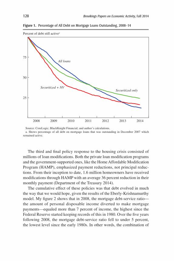
128 Brookings Papers on Economic Activity, Fall 2014
The third and final policy response to the housing crisis consisted of millions of loan modifications. Both the private loan modification programs and the government-supported ones, like the Home Affordable Modification Program (HAMP), emphasized payment reductions, not principal reduc-tions. From their inception to date, 1.6 million homeowners have received modifications through HAMP with an average 36 percent reduction in their monthly payment (Department of the Treasury 2014).
The cumulative effect of these policies was that debt evolved in much the way that we would hope, given the results of the Eberly-Krishnamurthy model. My figure 2 shows that in 2008, the mortgage debt-service ratio—the amount of personal disposable income diverted to make mortgage payments—equaled more than 7 percent of income, the highest since the Federal Reserve started keeping records of this in 1980. Over the five years following 2008, the mortgage debt-service ratio fell to under 5 percent, the lowest level since the early 1980s. In other words, the combination of
Securitized + NVSecuritized only
All loans
2008 2009 2010 2011 2012 2013 2014
25
50
75
Percent of debt still activea
Source: CoreLogic; BlackKnight Financial; and author’s calculations.a. Shows percentage of all debt on mortgage loans that was outstanding in December 2007 which
remained active.
Figure 1. Percentage of all debt on Mortgage loans outstanding, 2008–14

coMMenTs and discussion 129
private and public efforts in the aftermath of the crisis largely achieved the policy goal of reducing household mortgage payments.
reFerences For The Willen coMMenT
Department of the Treasury. 2014. “Making Home Affordable: Program Performance Report through the Third Quarter of 2014.” Washington. http://www.treasury.gov/initiatives/financial-stability/reports/Documents/3QMHAReportFinal.pdf
Federal Housing Finance Agency (FHFA), Office of Inspector General. 2012. “FHFA’s Oversight of the Enterprises Efforts to Recover Losses from Foreclosure Sales.” Audit Report no. 2013-001. http://fhfaoig.gov/Content/Files/AUD-2013-001.pdf
Fuster, Andreas, and Paul S. Willen. 2013. “Payment Size, Negative Equity, and Mortgage Default.” Working Paper no. 19345. Cambridge, Mass.: National Bureau of Economic Research.
1984 1988 1992 1996 2000 2004 2008 2012
4
5
6
7
Debt as percent of disposable income
Source: Board of Governors of the Federal Reserve System, http://www.federalreserve.gov/releases/housedebt/
a. The mortgage debt-service ratio is defined as payments due on all mortgage debt as a percentage of disposable personal income, seasonally adjusted.
Figure 2. Mortgage debt service ratio, 1980–2014a

130 Brookings Papers on Economic Activity, Fall 2014
Zandi, Mark. 2010. “The Economic Impact of Tax Cut Proposals: A Prudent Middle Course.” Moody’s Analytics Special Report, September. https://www.economy.com/mark-zandi/documents/Tax_Cuts_091510.pdf
GeneRAL DISCUSSIon John Haltiwanger thought the attention that Janice Eberly and Arvind Krishnamurthy paid to the impact of the hous-ing market collapse on consumption was worthwhile, but he suggested that a different mechanism may be equally relevant. In the Great Recession, young and small businesses were hammered in those places where hous-ing prices fell the most, to a degree that had not happened since 1980. The paper’s model has households using their balance sheets mainly to consume, but one could also examine a model in which households use their balances to start businesses. The implication is that the decline in household balance sheets may have contributed to the observed decline in the pace of entrepre-neurship in the Great Recession. Recent evidence shows that young firms are very important for job creation and productivity growth, so this impact of the housing market collapse is potentially quite important. He believes looking at this alternative mechanism might raise different questions about the kind of policy instruments the authors are thinking about.
Bradford DeLong said he remained mystified that conforming re- financing loans with equity kickers were not offered to all underwater and above-water homeowners alike. Instead, the debt overhang was removed through foreclosures and some case-by-case renegotiations. It was brutal, as discussant Paul Willen had acknowledged, and it is not clear that it is over yet. Even though during the housing bubble a million single-family homes above trend were being built each year, since 2007 the annual total has dropped to half a million, far below the long-run trend of 1.2 million a year. Now the country is 4 million single-family homes short, based on pre-housing-bubble trends, which translates into 4 million families liv-ing in makeshift situations, including relatives’ basements. Strangely, this enormous overhang is not exerting any pressure for a single-family hous-ing construction recovery. It is clear that both these potential homeowners and the lenders are unwilling to take on the types of risk they routinely took before 2008. Nevertheless, the single-family housing credit channel has not been restored to its old status. Is this a good finance pattern? Was the previous pattern a poor idea in the first place, or is the country now incurring enormous amounts of societal welfare losses?
Commenting on Willen’s discussant remarks, Robert Hall said the continuing decline in household debt service that Willen noted has

coMMenTs and discussion 131
brought with it a negative effect, since the debts are being paid off by forgoing consumption. The resulting consumption squeeze will not end until the debt-income ratio stabilizes. Hall also commented on discussant Austan Goolsbee’s remarks about what is preventing mortgage modifica-tions. Two phenomena are preventing it, Hall argued. One is the “sleeping dog”—that is, households unthinkingly continuing to service mortgages that were deeply underwater. Contrary to what the paper predicted, he agreed with Goolsbee that the number of such households was very large, and most of them have recovered as housing prices have recovered. The other barrier to modifications is what Hall called the “ringing phone syn-drome”: people simply no longer paying attention when lenders call to make a proposal. The very low number of modifications seems to sup-port this and explain why the modification programs failed. Nearly every affected household turned out to have either the sleeping dog or the ring-ing phone syndrome. Hall agreed with Goolsbee as well that the right approach would have been to set up a matching system to get people out of the houses they could not afford and into the right houses, but this fun-damentally necessary approach was never considered.
Benjamin Friedman thought it would be very useful to know why stra-tegic defaults have been as limited as they have been. For years—since the crisis began—economists have predicted that one would see a flood of stra-tegic defaults. And although it happened in a few places, nationwide the rate of strategic defaults has been far lower than expected.
Friedman also echoed what Goolsbee had said about the difference between losing one’s house to foreclosure in the recent crisis and what that used to mean in American life. The traditional notion involved losing some-thing a family had put its life savings into, and even though this also has happened recently, many of the people foreclosed on never had any invest-ment in their house to begin with. Many had bought homes with nearly 100 percent loan-to-value ratios. The discussion of this whole problem would be well served if this newer reality were more explicitly addressed.
Christopher Carroll noted that the paper’s authors use an elegant model, in the spirit of work by Gauti Eggertsson and Paul Krugman as well as work by Guido Lorenzoni and Ricardo Caballero, among others, in which the Great Recession’s big decline in consumption reflected liquidity prob-lems, with the banks cutting back on lending. However, Carroll said that if that had been the only story, now that the debt-to-income ratio has dropped enormously and banks are healthy again one would expect consumption to spring back again—yet it has not done so. In his view, what has happened is that uncertainty remains, and it seems to be even greater than it was

132 Brookings Papers on Economic Activity, Fall 2014
before. Before the Great Recession, risk premiums were at their lowest rates in recorded history, and confidence in the future was high.
Carroll argued that the difference in the degree of uncertainty between then and now is mostly responsible for the difference in the consumption and saving behavior. In 2007, the savings rate was 2 percent, according to the revised data, which was an all-time low. Therefore, perhaps one ought not ask why we have not returned to that period’s consumption and saving levels. Perhaps those levels were inappropriate. After financial crises, as Carmen Reinhart and Kenneth Rogoff have famously argued, the recover-ies tend to be very slow and drawn out. Carroll averred that this may be because after financial crises, uncertainty remains high for a long time, and this, rather than the banking sector’s more mechanical difficulties, may be what makes post-crisis recoveries so slow.
Robert Gordon recounted a personal story in which a new mortgage he had gotten in 2011 at a rate of 5.25 percent was offered to be refinanced two years later at just 2 5/8 percent on a 7-year ARM. His question was, Why are banks today so eager to offer windfall refinancing like that and reduce the amount they earn, yet so unwilling to do the same for lower-income homeowners who are underwater? As far as the high foreclosure rates, the damage one must also consider is what large numbers of foreclosures do to entire neighborhoods, where empty homes have to be torn down, as in Detroit. The true cost of foreclosure is that having vacant houses on one’s own block creates an externality. There is a loss of asset value in the whole economy that comes from the declining real value of these houses, and that in turn stems from the way the federal government and the banking system have treated so many people over the last seven years.
Responding to DeLong’s comments about the steep drop in home build-ing, Gordon suggested that another contributing cause is the trillion dol-lars in student debt that now burdens consumers. Simply put, many young people have moved back in with parents because of high student debt, which they cannot escape through bankruptcy. When one combines this reality with the country’s extremely slow wage growth and rapid growth in income inequality, one can see that the economy today has deep struc-tural problems.
Returning to the conundrum of the very low level of strategic defaults, Frederic Mishkin asked the authors how they built that into their model, given that it was an optimizing model. The gap between what economists expected before the recession regarding strategic defaults and what has actu-ally materialized has been very wide, so understanding why that has been the case may have important implications.

coMMenTs and discussion 133
Caroline Hoxby pointed out that the banks must have been able to see what Willen saw in his analysis as well, namely that after 5-year resets people were a lot less likely to default than they were after 7-year resets. She added that the banks must also have been aware that people like to stay in their own houses rather than strategically default, regardless of the reason. It remained difficult for her to understand, then, why the banks would not want to modify the payments in the short-term on their own, rather than worry about writing down the principal one way or the other. It might suggest that the banks felt that households were fundamentally mismatched with the houses they were paying mortgages on—but then, why had the banks lent them the money in the first place?
Wendy Edelberg said that to know whether principal write-downs might have been useful would depend on the timing. The first signs of pain in the housing market came before the persistent bad news that emerged in labor markets and with wages. In her view, if the causality ran from the prob-lems in the housing market to the subsequent problems in the labor market, the right solution would be to stop the foreclosures first. Another point is that people do not default only for strategic reasons, they can also default because life-cycle events occur that make it necessary for them to move.
When the housing crisis first happened, Edelberg related, many thought that if enough principal write-downs were done across the board, trou-bled homeowners could get out of mortgages without defaulting. But this turned out to be unrealistic. Echoing Goolsbee’s comment, Edelberg said it was generally expected that there would be losses and it was just a mat-ter of who was going to take them. A lot of people were in homes they could no longer afford or that were so big they never could afford them in the first place, but now with the price declines perhaps they could afford to buy them. The matching problem that Hall brought up was actually in many ways solved, in the sense that they belonged in the house they were already in, just at the new price.
Matthew Weinzierl picked up on the question of how people end up in bad mortgage debt situations in the first place. One dimension worth examining may be the policy choices buyers have and the incentives dif-ferent types of borrowers are given to take out loans that are too big. If a market has speculators trying to game the system and myopic buyers with a tendency to get in over their heads, that might reinforce the result that a payment modification is a better strategy, even in a general equilibrium sense, than principal reductions would be.
Looking back at the state of the housing market before the crisis, Jonathan Pingel noted that the misallocation of housing resources was connected

134 Brookings Papers on Economic Activity, Fall 2014
with house price expectations. It took a long time before people realized that home purchases were not going to remain a fantastic investment for-ever. Even as the crisis began, many thought the problem would remain a small one and that price appreciation would resume. Since a lot of the mis-allocation was a function of erroneous expectations, the important question now is how economists think about building such expectations into their own models.
Paul Willen said there is little evidence that people were diverting money from consumption to pay down debt. The Krugman-Eggertsson story is one in which the contract requires that when a home price goes down, the borrower has to make higher payments to reduce the level of debt, driving down consumption. But in fact, Willen said, U.S. mortgages are specifically designed so that changes in house prices have no effect on the repayment schedule of the mortgage. In other words, falling house prices do not force homeowners to divert money to pay down debt. Willen said he has seen little evidence that people are “curtailing” or voluntarily paying down their mortgages. Flow of Funds data show that considerable mortgage deleveraging has occurred but that it has largely resulted from write-downs by lenders and, to a lesser extent, scheduled amortization.
Arvind Krishnamurthy responded, first, by addressing strategic defaults. It seems to economists that strategic defaults should happen much more often than they do, he said, because they are making the error of treating the default choice as static, one in which the homeowner must decide “today.” But once one treats it as a dynamic problem, the intuition changes, because then one sees that the homeowner is weighing the choice of defaulting today against delaying defaulting until the next period. The only cost of that second choice is making another mortgage payment, a flow cost. So for a good portion of the equity space—the “underwaterness” space if you will—what the homeowner will choose is to continue to pay the flow cost, keeping the possibility that home prices rebound and the homeowner avoids default. It only becomes a better choice to default “now” if prices fall suf-ficiently low. This is why a reduction in the monthly payments can have a huge effect on the probability of default, as compared to a reduction in the principal, because in the former one is affecting the flow cost, and that is the most pertinent part of the choice.
Krishnamurthy acknowledged that Goolsbee’s psychological profiles, such as people simply not paying attention, might also help explain why some strategic default options were not taken. Nevertheless, he believed that the dynamics of exercising a “future” default option go quite far in helping one to understand why people often take a long while before defaulting.
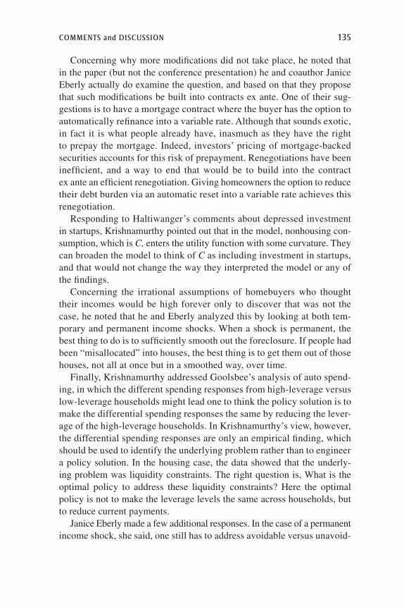
coMMenTs and discussion 135
Concerning why more modifications did not take place, he noted that in the paper (but not the conference presentation) he and coauthor Janice Eberly actually do examine the question, and based on that they propose that such modifications be built into contracts ex ante. One of their sug-gestions is to have a mortgage contract where the buyer has the option to automatically refinance into a variable rate. Although that sounds exotic, in fact it is what people already have, inasmuch as they have the right to prepay the mortgage. Indeed, investors’ pricing of mortgage-backed securities accounts for this risk of prepayment. Renegotiations have been inefficient, and a way to end that would be to build into the contract ex ante an efficient renegotiation. Giving homeowners the option to reduce their debt burden via an automatic reset into a variable rate achieves this renegotiation.
Responding to Haltiwanger’s comments about depressed investment in startups, Krishnamurthy pointed out that in the model, nonhousing con-sumption, which is C, enters the utility function with some curvature. They can broaden the model to think of C as including investment in startups, and that would not change the way they interpreted the model or any of the findings.
Concerning the irrational assumptions of homebuyers who thought their incomes would be high forever only to discover that was not the case, he noted that he and Eberly analyzed this by looking at both tem-porary and permanent income shocks. When a shock is permanent, the best thing to do is to sufficiently smooth out the foreclosure. If people had been “misallocated” into houses, the best thing is to get them out of those houses, not all at once but in a smoothed way, over time.
Finally, Krishnamurthy addressed Goolsbee’s analysis of auto spend-ing, in which the different spending responses from high-leverage versus low-leverage households might lead one to think the policy solution is to make the differential spending responses the same by reducing the lever-age of the high-leverage households. In Krishnamurthy’s view, however, the differential spending responses are only an empirical finding, which should be used to identify the underlying problem rather than to engineer a policy solution. In the housing case, the data showed that the underly-ing problem was liquidity constraints. The right question is, What is the optimal policy to address these liquidity constraints? Here the optimal policy is not to make the leverage levels the same across households, but to reduce current payments.
Janice Eberly made a few additional responses. In the case of a permanent income shock, she said, one still has to address avoidable versus unavoid-
136 Brookings Papers on Economic Activity, Fall 2014
able foreclosures. The paper addresses avoidable foreclosures, in which intervention should be designed to increase the homeowner’s consump-tion, reducing the probability of foreclosure. If a permanent shock has led to inefficient negotiations, those are the unavoidable foreclosures, and the best approach is simply to try to smooth them out.
One important challenge the paper does not address, she acknowledged, is the allocation of housing across space, something DeLong referred to. There is huge geographic heterogeneity both in where the foreclosures occur and where the housing demand is. The policies under consideration in this discussion do not help to smooth that aspect of the foreclosure problem, which constitutes one of the unresolved human costs in the hous-ing market that remain with us.