efficient calculation of the steepest descent direction for source-independent seismic waveform...

Journal of Computational Physics 208 (2005) 455–468

www.elsevier.com/locate/jcp

Efficient calculation of the steepest descent directionfor source-independent seismic waveform inversion:

An amplitude approach q

Yunseok Choi a,*, Changsoo Shin a, Dong-Joo Min b, Taeyoung Ha c

a Geophysical Prospecting Laboratory, School of Civil, Urban and Geosystem Engineering, Seoul National University,

S. Korea, San 56-1, Sillim-dong, Gwanak-gu, Seoul 151-742, Koreab Korea Ocean Research and Development Institute, S. Korea, 1270, Sa2-Dong, Sangrok-Gu, Ansan, Kyungki, 426-744, Korea

c Department of Mathematical Sciences, Seoul National University, S. Korea, San 56-1, Sillim-dong, Gwanak-gu, Seoul, 151-747, Korea

Received 5 May 2004; received in revised form 2 September 2004; accepted 29 September 2004

Available online 11 May 2005

Abstract

In seismic waveform inversion, if we have no information on source signature, we need to invert seismic data and

source signature either simultaneously or successively. In order to avoid the iterative update of the source signature in

waveform inversion based on classical, local optimization techniques, we propose two source-independent objective

functions using amplitude spectra of Fourier-transformed wavefields. One is constructed by normalizing the amplitude

spectra of observed data and modeled data with respect to the respective reference amplitudes. The other is achieved by

cross-multiplying the amplitude spectra of observed data and modeled data with the respective reference amplitudes. In

the computation of the steepest descent direction, we circumvent explicitly computing the Jacobian by employing a

matrix formalism of the wave equation in the frequency domain. Through numerical examples for the Marmousi

model, we demonstrate that our inversion algorithms can reproduce the subsurface velocity structure without estimat-

ing source signature.

� 2005 Elsevier Inc. All rights reserved.

Keywords: Waveform inversion; Source-independent objective function; Steepest descent direction; Local optimization; Jacobian

0021-9991/$ - see front matter � 2005 Elsevier Inc. All rights reserved.

doi:10.1016/j.jcp.2004.09.019

q This work was financially supported by the National Laboratory Project of the Ministry of Science and Technology, and the Brain

Korea 21 Project of the Ministry of Education.* Corresponding author. Tel.: +82 2 875 6292; fax: +82 2 875 6296.

E-mail addresses: [email protected] (Y. Choi), [email protected] (C. Shin), [email protected] (D.-J. Min), [email protected]

(T. Ha).

mailto:[email protected]




456 Y. Choi et al. / Journal of Computational Physics 208 (2005) 455–468

1. Introduction

Seismic inversion has been used to delineate the subsurface velocity structure from seismic data. Seismic

inversion has been mainly performed by traveltime tomography or waveform inversion. Traveltime tomog-

raphy of treating refraction or reflection events is performed on the basis of the kinematic property of seis-mic data [1–3], whereas waveform inversion employs the dynamic property of data [4,5]. Since traveltime

tomography is a high-frequency approximation, it cannot always describe the model whose velocity vari-

ations are similar to or less than source wavelength [5]. On the other hand, waveform inversion, which

is based on wave propagation, gives more refined velocity structures than traveltime tomography, although

waveform inversion requires more massive computation than traveltime tomography.

In the beginning, seismic inversion was mainly performed by directly calculating the Jacobian. Since

Lailly [6] and Tarantola [7] suggested using the backpropagation algorithm of reverse time migration

(e.g., the adjoint state of the wave equation) in seismic inversion, the backpropagation algorithm was exten-sively used to elegantly compute the steepest descent direction in waveform inversion [4,8–20].

Since full waveform inversion is performed by applying wave equation, we need to know exact source

signature to obtain a subsurface velocity structure that is compatible with true velocities. In the case of

the exact source wavelet not being known, we iteratively estimate source wavelet in addition to velocity

structure in waveform inversion algorithm. Zhou et al. [22] and Pratt [19] suggested methods of estimat-

ing source wavelet in waveform inversion algorithm, and found that the iteratively estimated source

wavelet is very sensitive to estimated velocity structure. As a solution to this problem, Zhou et al. [22]

suggested that successive inversions for source signature and velocity structure should be repeatedlyexecuted until reasonable solutions for both source signature and velocity structure can be obtained.

In order to avoid the additional work of inverting source wavelet, Lee and Kim [21] and Zhou and

Greenhalgh [5] proposed source-independent waveform inversion algorithms, which are based on the con-

ventional inversion technique directly computing the Jacobian. For the source-independent waveform

inversion algorithm, Lee and Kim [21] used the normalized wavefields with respect to a reference wave-

field in the frequency domain. The objective function constructed by Zhou and Greenhalgh [5] is similar

to that by Lee and Kim [21], except that Zhou and Greenhalgh [5] only used the amplitude spectrum

among spectral data obtained by the Fourier transform. Although Zhou and Greenhalgh [5] only usedamplitude spectra, they obtained realistic results in the inversion of crosshole data.

In this study, we propose two different source-independent amplitude inversion algorithms. One is con-

structed by normalizing the amplitudes of modeled data and field data with respect to amplitudes of the

respective reference wavefields like the method suggested by Zhou and Greenhalgh [5]. The other is ob-

tained by cross-multiplying the amplitudes of modeled wavefields and field data by the respective reference

amplitudes. In the former, the source wavelet is removed by deconvolution; in the latter, the source wavelet

is eliminated by convolution. The main characteristic of our waveform inversion techniques is related to the

computation of the steepest descent direction. In the following sections, we construct the two source-inde-pendent objective functions, and show how to compute the steepest descent direction in the source-indepen-

dent waveform inversion algorithms. In order to demonstrate our waveform inversion algorithms, we

present numerical examples for the Marmousi synthetic data.

2. Theory

2.1. The first source-independent objective function using deconvolution

In the frequency domain, since time series are expressed by the amplitude and phase spectra, we can

write the observed data as

Y. Choi et al. / Journal of Computational Physics 208 (2005) 455–468 457

~di;jðxÞ ¼ Adi;je

ihdi;j ; i ¼ 1; 2; . . . ;m; j ¼ 1; 2; . . . ; n; ð1Þ

where x is the angular frequency, Adi;jðxÞ and hdi;jðxÞ are the amplitude and phase spectra of the ob-

served data, respectively, and i and j denote the source and receiver points, respectively. The superscript

d is used to discriminate the field data from the modeled data that will be indicated by the superscript

u. If we consider ideal, 2D acoustic media without intrinsic attenuation, seismic data observed at thesurface are defined as the convolution of the source wavelet and the impulse response in the time

domain:

di;jðtÞ ¼ wðtÞ � ri;jðtÞ; ð2Þ

where w(t) is the source wavelet and ri,j(t) is the impulse response. The frequency-domain relation corre-

sponding to Eq. (2) is given as

~di;jðxÞ ¼ ~wðxÞ~ri;jðxÞ. ð3Þ

In Eq. (3), we note that the amplitude Adi;j of Eq. (1) is composed of amplitudes of source wavelet and

impulse response, as follows:

Adi;jðxÞ ¼ sdðxÞadi;jðxÞ; ð4Þ

where sdðxÞ and adi;jðxÞ are the amplitudes of source wavelet and impulse response for the observed data,respectively.

If we arbitrarily choose a reference wavefield and normalize observed wavefields with respect to the ref-

erence wavefield just for amplitude spectra, we obtain

j~di;jðxÞjj~di;refðxÞj

¼Adi;jðxÞ

Adi;refðxÞ

¼sdðxÞadi;jðxÞsdðxÞadi;refðxÞ

¼adi;jðxÞadi;refðxÞ

; ð5Þ

where the subscript ref indicates the reference data. In Eq. (5), since source wavelet is the same, we obtain

the source-independent amplitude ratio.

Similarly, we can represent the normalized amplitude of the modeled data as

j~ui;jðxÞjj~ui;refðxÞj

¼Aui;jðxÞ

Aui;refðxÞ

¼suðxÞaui;jðxÞsuðxÞaui;refðxÞ

¼aui;jðxÞaui;refðxÞ

; ð6Þ

where the superscript u indicates the modeled data.

For source-independent waveform inversion, we define the objective function as l2 norm of residuals be-

tween normalized amplitudes of field data and modeled data with respect to the respective reference ampli-

tudes. The objective function is expressed for a single frequency as

E ¼Xi

Xj

1

2

Aui;j

Aui;ref

�Adi;j

Adi;ref

" #2. ð7Þ

The model parameter minimizing the objective function is obtained by computing the derivative of Eq. (7)

with respect to the kth model parameter pk, as follows:

oEopk

¼Xi

Xj

Aui;j

Aui;ref

�Adi;j

Adi;ref

!o

opk

Aui;j

Aui;ref

!; ð8Þ

where the derivative of amplitude with respect to pk is given as


o

opk

Aui;j

Aui;ref

!¼ 1

Aui;ref

oAui;j

opk

� ��

Aui;j

Aui;ref

� �2 oAui;ref

opk. ð9Þ

We can compute the partial derivative of amplitude with respect to model parameter pk using partial deriv-ative of the modeled wavefield with respect to pk. The partial derivative of the modeled wavefield divided by

the modeled wavefield can be written as

1

~ui;j

o~ui;jopk

¼ 1

Aui;j

oAui;j

opkþ i

ohui;jopk

; ð10Þ

and then the partial derivative of amplitude is defined as

oAui;j

opk¼ Au

i;jRe1

~ui;j

o~ui;jopk

� �. ð11Þ

Substituting Eqs. (9) and (11) into Eq. (8) gives

oEopk

¼Xi

Xj

ReAui;j

Aui;ref

�Adi;j

Adi;ref

!1

Aui;ref

Aui;j

~ui;j

o~ui;jopk

(� 1

Aui;ref~ui;ref

o~ui;refopk

Aui;j

Aui;ref

�Adi;j

Adi;ref

!Aui;j

); ð12Þ

which can be rewritten in a matrix form as

oEopk

¼X

iRe

1

Aui;ref

o~uiopk

� �TAui;1

~ui;1

Aui;1

Aui;ref

� Adi;1

Adi;ref

� �Aui;2

~ui;2

Aui;2

Aui;ref

� Adi;2

Adi;ref

� �

..

.

Aui;n

~ui;n

Aui;n

Aui;ref

� Adi;n

Adi;ref

� �

266666666664

377777777775� Ci;ref

Aui;ref

o~uiopk

� �T0

..

.

1~ui;ref

0

..

.

266666664

377777775

8>>>>>>>>>><>>>>>>>>>>:

9>>>>>>>>>>=>>>>>>>>>>;

ð13Þ

with

Ci;ref ¼Xj

Aui;j

Aui;ref

�Adi;j

Adi;ref

!Aui;j

" #. ð14Þ

We can rewrite the gradient vector as

oEopk

¼Xi

Re1

Aui;ref

o~uiopk

� �Tri

( ); ð15Þ

where ri is the residual vector whose components are expressed as

ri;j ¼

Aui;j

~ui;j

Aui;j

Aui;ref

� Adi;j

Adi;ref

� �; j 6¼ ref ;

Aui;j

~ui;j

Aui;j

Aui;ref

� Adi;j

Adi;ref

� �� Ci;ref

~ui;ref; j ¼ ref.

8>>><>>>:

ð16Þ

In Eqs. (15) and (16), if we compute the partial derivative wavefield for an entire model parameter and aug-ment the residual vector by adding zeroes, we can express the total gradient for the entire model parameter

as


oEop

¼Xi

Re1

Aui;ref

o~uiop

� �Tri

( )ð17Þ

with

ri;k ¼

Aui;k

~ui;k

Aui;k

Aui;ref

� Adi;k

Adi;ref

� �; k ¼ j and k 6¼ ref ;

Aui;k

~ui;k

Aui;k

Aui;ref

� Adi;k

Adi;ref

� �� Ci;ref

~ui;ref; k ¼ j and k ¼ ref ;

0; k 6¼ j;

8>>>>><>>>>>:

ð18Þ

where j indicates the receiver point.

In Eq. (17), the partial derivatives of the modeled wavefields can be expressed by using the forward mod-

eling operator S and the virtual source matrix V, as they are in the reverse-time migration (e.g., Eqs. (A.8)–

(A.12) in Appendix A) [26], which results in

oEop

¼Xi

Xx

Re1

Aui;ref

VTi ½S

�1�Tri

( )Dx ð19Þ

for the entire frequency. By comparing Eq. (19) with Eq. (A.11) for the reverse-time migration, we cannote that the source-independent waveform inversion has the same numerical algorithm as that of the

reverse-time migration. In Eq. (19), since the forward modeling operator S is symmetric and the self

adjoint, the term [S�1]Tri implies backpropagating the residuals. As a result, we can determine the steep-

est descent direction by backpropagating the residuals between normalized amplitudes of observed data

and modeled data, and then convolving the backpropagated residuals with the virtual source (e.g.,

Appendix A; [26]).

In this source-independent waveform inversion, we note that the reference wavefields can be arbitrarily

chosen among wavefields observed or computed at all the receiver points. As an alternative of the inversion,we can also repeat the inversion process one by one so that wavefields of all the receivers can be the refer-

ence wavefield, and then average the resulting velocity models.

2.2. Source-independent objective function using convolution

An alternative to building a source-independent objective function is to cross-multiply both observed

data and modeled data by the respective reference amplitudes. In this case, the objective function can be

given at a single frequency as

E ¼Xi

Xj

1

2Adi;refðxÞAu

i;jðxÞ � Aui;refðxÞAd

i;jðxÞh i2

¼Xi

Xj

1

2adi;refðxÞsdðxÞaui;jðxÞsuðxÞ � aui;refðxÞsuðxÞadi;jðxÞsdðxÞh i2

. ð20Þ

Since the amplitudes of source wavelets for both observed data and modeled data are included in both

terms, the source effect also disappears in this objective function. Similarly to the former source-indepen-

dent waveform inversion using deconvolution, we can compute the steepest descent direction for the entire

frequency by using

oEop

¼Xi

Xx

Re VTi ½S

�1�Trin o

Dx ð21Þ


with the residual vector

ri;k ¼

Adi;refA

ui;k

~ui;kAdi;refA

ui;k � Au

i;refAdi;k

� �; k ¼ j and k 6¼ ref ;

Adi;refA

ui;k

~ui;kAdi;refA

ui;k � Au

i;refAdi;k

� �� C0

i;ref

~ui;ref; k ¼ j and k ¼ ref ;

0; k 6¼ j;

8>>><>>>:

ð22Þ

where

C0i;ref ¼

Xj

Aui;refA

di;j Ad

i;refAui;j � Au

i;refAdi;j

h i. ð23Þ

In this source-independent objective function using convolution, we also propagate the residuals of

weighted amplitudes, and then compute the gradient vector by calculating the zero-lag value of convolutionbetween the backpropagated residual and the virtual source.

3. Numerical examples

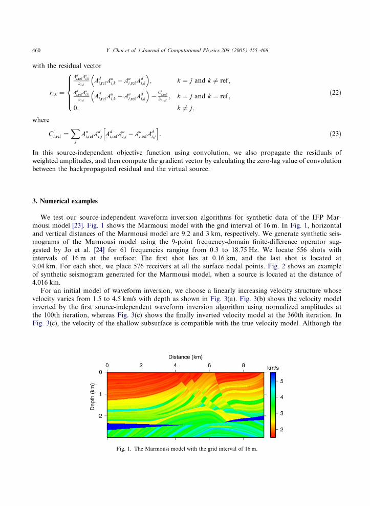
We test our source-independent waveform inversion algorithms for synthetic data of the IFP Mar-

mousi model [23]. Fig. 1 shows the Marmousi model with the grid interval of 16 m. In Fig. 1, horizontal

and vertical distances of the Marmousi model are 9.2 and 3 km, respectively. We generate synthetic seis-mograms of the Marmousi model using the 9-point frequency-domain finite-difference operator sug-

gested by Jo et al. [24] for 61 frequencies ranging from 0.3 to 18.75 Hz. We locate 556 shots with

intervals of 16 m at the surface: The first shot lies at 0.16 km, and the last shot is located at

9.04 km. For each shot, we place 576 receivers at all the surface nodal points. Fig. 2 shows an example

of synthetic seismogram generated for the Marmousi model, when a source is located at the distance of

4.016 km.

For an initial model of waveform inversion, we choose a linearly increasing velocity structure whose

velocity varies from 1.5 to 4.5 km/s with depth as shown in Fig. 3(a). Fig. 3(b) shows the velocity modelinverted by the first source-independent waveform inversion algorithm using normalized amplitudes at

the 100th iteration, whereas Fig. 3(c) shows the finally inverted velocity model at the 360th iteration. In

Fig. 3(c), the velocity of the shallow subsurface is compatible with the true velocity model. Although the

Fig. 1. The Marmousi model with the grid interval of 16 m.


deeper subsurface also converges with the true velocity model as the iteration increases, the reservoir and its

neighboring structure are not clearly seen in the finally inverted velocity model. Furthermore, the left and

the right part of the inverted velocity structure are still far from the true velocity structure. Fig. 4 shows the

history of rms error. The rms error slowly decreases as the inverted velocity approximates the true velocity

model.Fig. 5(a) and (b) shows the velocity models inverted by the second source-independent inversion algo-

rithm using convolution at the 100th and 360th iterations, respectively. From Fig. 5(b), we note that the

inverted velocity model is almost the same as that of the first objective function using normalized amplitude

(e.g., Fig. 3(c)). Fig. 6 shows the history of rms error, which is also similar to that of the first objective

function.

In general, since low-frequency components of real data are mixed with noise, we often discard low-

frequency components less than 5 Hz in seismic data processing. In order to investigate if our algorithm

can be applied to data that are lacking low-frequency components, we also test the first inversion algo-rithm using deconvolution for the Marmousi synthetic data without frequencies less than 5 Hz. Fig. 7

shows the inverted velocity model at the 250th iteration. By comparing Fig. 7 to Fig. 3(c), we note that

although shallow subsurface structure is comparable to the true velocity model, the resolution of the

Fig. 2. A synthetic seismogram generated by using 9-point frequency-domain finite-difference operator for the Marmousi model, when

a source is located at 4.016 km.

Fig. 3. Numerical examples of the first source-independent waveform inversion using deconvolution for the Marmousi model: (a)

initial velocity model, (b) the 100th inverted velocity model and (c) the 360th inverted velocity model.


whole structure is not as good as that obtained by using the entire frequency band. Fig. 8 shows the

history of rms error. In Fig. 8 we see that the rms error decreases to 10% of initial value, which is larger

than that of entire frequency data.

Fig. 5. Numerical examples of the second, source-independent waveform inversion using convolution for the Marmousi model: (a) the

100th and (b) 360th inverted velocity models.

0 100 200 300 400Iteration number

0e+00

5e–05

1e–04

RM

S e

rror

Fig. 4. The history of rms error in the first source-independent waveform inversion using deconvolution.


0 100 200 300Iteration number

0.0e+00

5.0e–05

1.0e–04

1.5e–04

RM

S e

rror

Fig. 8. The history of rms error in the first, source-independent waveform inversion for the Marmousi synthetic data without low-

frequency information less than 5 Hz.

Fig. 7. The velocity model inverted by the first, source-independent waveform inversion for the Marmousi synthetic data without low-

frequency information less than 5 Hz at the 250th iteration.

0 100 200 300 400

Iteration number

0e+00

1e–16

2e–16

3e–16

RM

S e

rror

Fig. 6. The history of rms error in the second, source-independent waveform inversion using convolution.



4. Conclusion

We presented two source-independent seismic inversion algorithms employing amplitude spectra of Fou-

rier-transformed wavefields. In our algorithms, we constructed source-independent objective functions by

either deconvolution (expressed by dividing in the frequency domain) or convolution (described by multi-plying in the frequency domain). In the case of deconvolution, we normalized amplitudes of modeled data

and observed data with respect to the respective reference amplitudes and then defined the objective func-

tion as the l2 norm between residuals of the normalized amplitudes. On the other hand, in the case of con-

volution, we cross-multiplied amplitudes of modeled data and observed data with the respective reference

amplitudes. The reference wavefield can be arbitrarily chosen among wavefields at surface receiver points.

For the calculation of the steepest descent direction, we did not directly compute the Jacobian, but used the

backpropagation technique of reverse time migration on the basis of the symmetry of Green�s function. Thenumerical algorithm of our inversion techniques is equivalent to that of conventional pre-stack reverse timemigration and waveform inversion.

From numerical examples for the Marmousi synthetic data, we note that our inversion algorithm gives

inverted velocity structures compatible with true velocity models without numerically estimating source sig-

nature. In order to demonstrate the feasibility of our algorithm to real data, we also tested our algorithms

for the Marmousi synthetic data without low frequencies less than 5 Hz. In this case, although the velocity

model inverted without low frequencies is not as good as that of whole frequency data, the inverted velocity

structure is still comparable to the true velocity structure. In spite of these numerical examples, we still hes-

itate to assert that our source-independent waveform inversion algorithms can be applied to real data col-lected in the 3D elastic media causing mode conversion, scattering, and intrinsic attenuation, because we

construct our algorithms on the assumption of the ideal, 2D acoustic media. Application of our algorithms

to real data may require some correction for 3D elastic effects, a topic that will be studied in the future.

Considering that the waveform inversion employs the same numerical algorithm as reverse time migra-

tion, we expect that our source-independent algorithm can be applied to the reverse-time migration without

estimating the source wavelet. In the future, we will apply our source-independent algorithm to 2D elastic,

3D acoustic, and 3D elastic waveform inversions. We can also extend our algorithm to time-domain wave-

form inversions.

Appendix A. Reverse time migration

We examine numerical algorithm of 2D reverse-time migration following the 1D reverse-time migration

algorithm presented by Shin et al. [26]. Since the partial derivative wavefield with respect to the model

parameter can be interpreted as the sensitivity of wavefields to the perturbation of model parameter [27],

we can establish a numerical expression of the migrated image for the kth model parameter, as follows:

/k ¼Xi

Xj

Xt

oui;jðtÞopk

di;jðtÞ; i ¼ 1; 2; . . . ;Ns; and j ¼ 1; 2; . . . ;Nr; ðA:1Þ

where ui,j and di,j are the modeled data and the observed data, respectively, and i and j indicate the source

and receiver points, respectively.

In the frequency domain, the equivalent of Eq. (A.1) can be written as

/k ¼Xi

Xj

Xx

o~ui;jðxÞopk

~d�i;jðxÞ ðA:2Þ

or


/k ¼Xi

Xj

Xx

o~u�i;jðxÞopk

~di;jðxÞ; ðA:3Þ

where ~di;jðxÞ and ½o~ui;jðxÞ=opk� are the Fourier transforms of di,j(t) and [oui,j(t)/opk], respectively, and * de-

notes the complex conjugate. For convenience, we consider a single frequency, which allows us to omit the

summation about frequency.

In Eq. (A.2), the migrated image is described by the field data observed at the surface receiver points and

the partial derivative wavefields computed at the surface receiver points. We can rewrite Eq. (A.2) by using

the partial derivative wavefield for an entire model parameter, as follows:

U ¼Xi

o~ui;1ðxÞop1

� � � o~ui;Nr ðxÞop1

o~ui;Nrþ1ðxÞ

op1� � � o~ui;K ðxÞ

op1

o~ui;1ðxÞop2

� � � o~ui;Nr ðxÞop2

o~ui;Nrþ1ðxÞ

op2� � � o~ui;K ðxÞ

op2

..

. ... ..

. . .. ..

.

o~ui;1ðxÞopK

� � � o~ui;Nr ðxÞopK

o~ui;Nrþ1ðxÞ

opK� � � o~ui;K ðxÞ

opK

266666664

377777775

~d�i;1ðxÞ

..

.

~d�i;Nr

ðxÞ0

..

.

0

2666666666664

3777777777775. ðA:4Þ

Eq. (A.4) can be expressed in a matrix form as

U ¼Xi

o~uiðxÞop

� �Tr�i ðxÞ ðA:5Þ

with

ri;kðxÞ ¼~di;kðxÞ; k ¼ j;

0; k 6¼ j;

(ðA:6Þ

where j indicates the surface receiver point.In a similar method, Eq. (A.3) can be expressed as

U ¼Xi

o~u�i ðxÞop

� �TriðxÞ. ðA:7Þ

The partial derivative wavefields in Eqs. (A.5) and (A.7) can be computed by taking the derivative of the

matrix equation given in forward modeling.

In forward modeling of wave equation using frequency-domain finite-difference or finite-element meth-

ods, we solve the discretized matrix equation written for a single frequency by

SðxÞ~uiðxÞ ¼ f iðxÞ; ðA:8Þ
where S(x) is the complex impedance matrix and fi(x) is the ith source vector [25]. Taking the partial deriv-
ative of Eq. (A.8) with respect to the kth model parameter pk gives

SðxÞ o~uiðxÞopk

¼ � oSðxÞopk

~uiðxÞ oro~uiðxÞopk

¼ S�1ðxÞvi;kðxÞ ðA:9Þ

with

vi;kðxÞ ¼ � oSðxÞopk

~uiðxÞ; ðA:10Þ

where vi,k(x) is defined as the virtual source vector with respect to the kth model parameter [4].


On the basis of Eqs. (A.9) and (A.10), we can rewrite Eqs. (A.5) and (A.7) for an entire frequency band

as

U ¼Xi

Xx

VTi ðxÞ½S

�1ðxÞ�Tr�i ðxÞ ðA:11Þ

or

U ¼Xi

Xx

V�Ti ðxÞ½S�1ðxÞ��TriðxÞ; ðA:12Þ

where Vi(x) is the ith virtual source matrix, whose column is the virtual source vector vi,k(x) with respect to

the kth model parameter:

ViðxÞ ¼ vi;1ðxÞvi;2ðxÞ � � � vi;N ðxÞ½ �. ðA:13Þ
Note that the complex conjugate in the frequency domain represents time-reverse in the time domain, and
the forward modeling operator S is symmetric. Then, the product of the last two terms ½S�1ðxÞ�Tr�i ðxÞ inEq. (A.11) describes downward-propagation of the time-reverse surface wavefield. In Eq. (A.11), we can

obtain a migrated image by downward propagating time-reversed surface wavefields and then convolving

the downward-propagated wavefields with the virtual source. Similarly, in Eq. (A.12), a migrated image is

obtained by backpropagating normal (unreversed) surface wavefields and then taking the zero-lag cross-

correlation between the backpropagated wavefields and the virtual source. Eq. (A.12) is a general fre-

quency-domain expression of reverse-time migration that is mainly implemented by time-reversed marchingof surface data in the time domain. In the frequency domain, however, we favor Eq. (A.11), which is an

alternative expression of reverse-time migration.

References

[1] G. Nolet, Seismic Wave Propagation and Seismic Tomography with Applications in Global Seismology and Exploration

Geophysics, Reidel, Dordrecht, 1987.

[2] N.D. Bregman, R.C. Bailey, C.H. Chapman, Crosshole seismic tomography, Geophysics 54 (1989) 200–215.

[3] Y. Luo, G.T. Schuster, Wave-equation traveltime inversion, Geophysics 56 (1991) 645–653.

[4] R.G. Pratt, C.S. Shin, G.J. Hicks, Gauss–Newton and full Newton methods in frequency-space seismic waveform inversion,

Geophys. J. Int. 133 (1998) 341–362.

[5] B. Zhou, S.A. Greenhalgh, Crosshole seismic inversion with normalized full-waveform amplitude data, Geophysics 68 (2003)

1320–1330.

[6] P. Lailly, The seismic inverse problem as a sequence of before stack migration, in: J.B. Bednar, R. Redner, E. Robinson, A.

Weglein (Eds.), Conference on Inverse Scattering: Theory and Application, Soc. Industr. Appl. Math (1983).

[7] A. Tarantola, Inversion of seismic reflection data in the acoustic approximation, Geophysics 49 (1984) 1259–1266.

[8] A. Bamberger, G. Chavent, C. Hemon, P. Lailly, Inversion of normal incidence seismograms, Geophysics 46 (1982) 757–770.

[9] P. Kolb, F. Collino, P. Lailly, Prestack inversion of a 1-D mdium, Proc. IEEE 74 (1986) 498–506.

[10] O. Gauthier, J. Vriieux, A. Tarantola, Two-dimensional nonlinear inversion of seismic waveforms: numerical results, Geophysics

51 (1986) 1387–1403.

[11] A. Trantola, A strategy for nonlinear elastic inversion of seismic reflection data, Geophysics 51 (1986) 1893–1903.

[12] A. Trantola, G. Jobert, D. Trezeguet, E. Denelle, The nonlinear inversion of seismic waveforms can be performed either time

extrapolation or by depth extrapolation, Geophys. Prospect. 36 (1988) 383–416.

[13] P. Mora, Nonlinear two-dimensional elastic inversion of multioffset seismic data, Geophysics 52 (1987) 1211–1228.

[14] R. Sun, G.A. McMechan, Full-wavefield inversion of wide-aperture SH and Love wave data, Geophys. J. Int. 111 (1992) 1–10.

[15] D. Cao, W.B. Beydoun, S.C. Singh, A. Trantola, A simultaneous inversion for background velocity and impedance maps,

Geophysics 55 (1990) 458–469.

[16] A. Pica, J.P. Diet, A. Tarantola, Nonlinear inversion of seismic reflection data in a laterally invariant medium, Geophysics 55

(1990) 284–292.

[17] T. Xu, G.A. McMechan, R. Sun, 3-D pretack full-wavefield inversion, Geophysics 60 (1995) 1805–1818.


[18] C. Zhou, W. Cai, Y. Luo, G.T. Schuster, S. Hassanzadeh, Acoustic wave equation traveltime and waveform inversion of cross

hole seismic data, Geophysics 60 (1995) 765–773.

[19] R.G. Pratt, Seismic waveform inversion in the frequency domain, Part 1: Theory and verification in a physical scale model,

Geophysics 64 (1999) 888–901.

[20] R.G. Pratt, R.M. Shipp, Seismic waveform inversion in the frequency domain, Part 2: Falt delineation in sediments using

crosshole data, Geophysics 64 (1999) 902–914.

[21] K.H. Lee, H.J. Kim, Source-independent full-waveform inversion of seismic data, Geophysics 68 (2003) 2010–2015.

[22] C. Zhou, G.T. Schuster, S. Hassanzadeh, J.M. Harris, Elastic wave equation traveltime and waveform inversion of crosswell data,

Geophysics 62 (1997) 853–869.

[23] R. Versteeg, The Marmousi experience: Velocity model determination on a synthetic complex data set, The Leading Edge 13

(1994) 927–936.

[24] C.H. Jo, C.S. Shin, J.H. Suh, Design of an optimal 9 point finite difference frequency-space acoustic wave equation scheme for

inversion and modeling, Geophysics 61 (1996) 329–337.

[25] K.J. Marfurt, Accuracy of finite-difference and finite-element modeling of the scalar and elastic wave-equations, Geophysics 49

(1984) 533–549.

[26] C. Shin, D.-J. Min, D. Yang, S.K. Lee, Evaluation of poststack migration in terms of virtual source and partial derivative

wavefields, J. Seism. Explor. 12 (2003) 17–37.

[27] C. Shin, S. Chung, Understanding CMP stacking hyperbola in terms of partial derivative wavefield, Geophysics 64 (1999) 1774–

1782.

efficient calculation of the steepest descent direction for source-independent seismic waveform...

Documents