efficient and secure network services in wireless sensor networks
TRANSCRIPT
EFFICIENT AND SECURE NETWORK SERVICES INWIRELESS SENSOR NETWORKS
by
Min-gyu Cho
A dissertation submitted in partial fulfillmentof the requirements for the degree of
Doctor of Philosophy(Computer Science and Engineering)
in The University of Michigan2009
Doctoral Committee:
Professor Kang G. Shin, ChairProfessor Atul PrakashAssociate Professor Sugih JaminAssociate Professor Mingyan Liu

c© Min-gyu Cho 2009
All Rights Reserved

ACKNOWLEDGEMENTS
First of all, I would like to express my gratitude to my advisor, Professor Kang G.
Shin. Without his continuous guidance and encouragement, I could never have completed
my dissertation. I would also like to thank my other committee members, Professors Atul
Prakash, Sugih Jamin, and Mingyan Liu. Thanks to their invaluable comments, I could
significantly improve the quality of my dissertation.
I thank great colleagues at the Real-Time Computing Laboratory including Songkuk
Kim, Jai-jin Lim, Taejoon Park, Kyu-Han Kim, Jisoo Yang, Hyoil Kim, Zhigang Chen,
Alex Min, Antino Kim, Sangsoo Park, Youngjune Choi, Katharine Chang, and Buyoung
Yun. I am grateful for what they shared with me professionally and personally over the
years of my graduate study.
I have been very fortunate to share life-enriching friendship with special people. With
wonderful memories with them, my long journey during my graduate study has been much
more enjoyable and endurable. My special thanks go to Sang-hyun Kim, Kijung Kim,
Kyunghoon Min, Hongseok Kim, Joongho Won, Kyung-Joon Park, Jiyoun Kim, Minjoong
Kim, Jungkeun Yoon, Hyunmin Kang, Goo Jun, Yang-won Jung, Eunjin Jung, Jooyong
Jun, Sangwoo Lee, Wook Chang, Daeho Lee, Yoonna Oh, Taemin Earmme, and Jiwon
Kim.
Last but not least, I would like to express my deepest love to my parents for their endless
love and support for my whole life.
ii

TABLE OF CONTENTS
ACKNOWLEDGEMENTS . . . . . . . . . . . . . . . . . . . . . . . . . . . . ii
LIST OF FIGURES . . . . . . . . . . . . . . . . . . . . . . . . . . . . . . . . vi
LIST OF TABLES . . . . . . . . . . . . . . . . . . . . . . . . . . . . . . . . . x
ABSTRACT . . . . . . . . . . . . . . . . . . . . . . . . . . . . . . . . . . . . . xi
CHAPTER
I. INTRODUCTION . . . . . . . . . . . . . . . . . . . . . . . . . . . . . . 1
1.1 Overview of Wireless Sensor Networks . . . . . . . . . . . . . . . 11.2 Existing Network Services . . . . . . . . . . . . . . . . . . . . . 2
1.2.1 Localization . . . . . . . . . . . . . . . . . . . . . . . . 21.2.2 Geographic forward routing . . . . . . . . . . . . . . . 41.2.3 Data-Centric Storage . . . . . . . . . . . . . . . . . . . 51.2.4 Time Synchronization . . . . . . . . . . . . . . . . . . 6
1.3 Motivation and Contributions . . . . . . . . . . . . . . . . . . . . 61.3.1 Distributed Location Service Protocol . . . . . . . . . . 61.3.2 Distributed Hole Detection . . . . . . . . . . . . . . . . 71.3.3 Attack-Resilient Collaborative Message Authentication . 8
1.4 Architecture of Sensor Network Applications . . . . . . . . . . . . 81.5 Outline . . . . . . . . . . . . . . . . . . . . . . . . . . . . . . . . 9
II. DISTRIBUTED LOCATION SERVICE PROTOCOL . . . . . . . . . 11
2.1 Introduction . . . . . . . . . . . . . . . . . . . . . . . . . . . . . 112.1.1 Background . . . . . . . . . . . . . . . . . . . . . . . . 122.1.2 Proposed Approach . . . . . . . . . . . . . . . . . . . . 15
2.2 Distributed Location Service Protocol . . . . . . . . . . . . . . . . 172.2.1 Selection and Update of Location Servers . . . . . . . . 172.2.2 Processing of Location Queries . . . . . . . . . . . . . 19
2.3 Conditions for High Packet-Delivery Ratio . . . . . . . . . . . . . 20
iii
2.3.1 Conditions for High Packet-Delivery Ratio under DLSP 212.3.2 Configuration of Protocol Parameters for DLSP . . . . . 242.3.3 Choice of Design Paradigm . . . . . . . . . . . . . . . 25
2.4 Analysis of Location-Service Overhead . . . . . . . . . . . . . . . 262.4.1 Analysis of Location-Update Overhead . . . . . . . . . 262.4.2 Optimization of DLSP . . . . . . . . . . . . . . . . . . 27
2.5 Adaptation of Location Service . . . . . . . . . . . . . . . . . . . 282.5.1 Adaptive Location Updates . . . . . . . . . . . . . . . . 292.5.2 Condition for High Query-Delivery Ratio . . . . . . . . 302.5.3 Analysis of Overall Energy-Efficiency . . . . . . . . . . 322.5.4 Comparison of Hierarchical Location Services . . . . . 32
2.6 Evaluation . . . . . . . . . . . . . . . . . . . . . . . . . . . . . . 322.6.1 The Simulation Setup . . . . . . . . . . . . . . . . . . . 332.6.2 Simulation Results Using 802.11 MAC . . . . . . . . . 352.6.3 Simulation Results Using S-MAC . . . . . . . . . . . . 412.6.4 Results with Additional Mobility Models . . . . . . . . 432.6.5 Results on Robustness Against Node Failures . . . . . . 452.6.6 Results on Robustness with Low Densities . . . . . . . 47
2.7 Conclusion . . . . . . . . . . . . . . . . . . . . . . . . . . . . . . 48
III. DISTRIBUTED HOLE DETECTION . . . . . . . . . . . . . . . . . . 50
3.1 Introduction . . . . . . . . . . . . . . . . . . . . . . . . . . . . . 503.2 Related Work . . . . . . . . . . . . . . . . . . . . . . . . . . . . 523.3 System Assumptions . . . . . . . . . . . . . . . . . . . . . . . . . 54
3.3.1 Radio Model . . . . . . . . . . . . . . . . . . . . . . . 543.3.2 Localization Service Model . . . . . . . . . . . . . . . 56
3.4 Distributed Hole Detection . . . . . . . . . . . . . . . . . . . . . 573.4.1 Overview . . . . . . . . . . . . . . . . . . . . . . . . . 573.4.2 Definition of a Hole . . . . . . . . . . . . . . . . . . . 573.4.3 Identification of Candidate Nodes . . . . . . . . . . . . 603.4.4 Handling Special Cases . . . . . . . . . . . . . . . . . . 623.4.5 Identification of hole boundary . . . . . . . . . . . . . . 633.4.6 Detection of Topology Changes . . . . . . . . . . . . . 67
3.5 Geographic Forward Routing with Hole Avoidance . . . . . . . . 673.5.1 Overview . . . . . . . . . . . . . . . . . . . . . . . . . 673.5.2 Detouring Messages Using Hole Information . . . . . . 68
3.6 Evaluation . . . . . . . . . . . . . . . . . . . . . . . . . . . . . . 713.6.1 Distributed Hole Detection . . . . . . . . . . . . . . . . 713.6.2 Geographic Forward Routing with Hole Avoidance . . . 77
3.7 Conclusion . . . . . . . . . . . . . . . . . . . . . . . . . . . . . . 80
IV. ATTACK-RESILIENT COLLABORATIVE MESSAGE AUTHENTI-CATION . . . . . . . . . . . . . . . . . . . . . . . . . . . . . . . . . . . 83
iv
4.1 Introduction . . . . . . . . . . . . . . . . . . . . . . . . . . . . . 834.2 Related Work . . . . . . . . . . . . . . . . . . . . . . . . . . . . 864.3 System Model . . . . . . . . . . . . . . . . . . . . . . . . . . . . 89
4.3.1 Sensor Network Model . . . . . . . . . . . . . . . . . . 894.3.2 Attack Models . . . . . . . . . . . . . . . . . . . . . . 90
4.4 Key Management . . . . . . . . . . . . . . . . . . . . . . . . . . 924.4.1 Polynomial-based Key Pre-distribution . . . . . . . . . 924.4.2 Key Distribution . . . . . . . . . . . . . . . . . . . . . 934.4.3 Key Assignment . . . . . . . . . . . . . . . . . . . . . 94
4.5 Attack-Resilient Collaborative Message Authentication (ARCMA) 964.5.1 Overview . . . . . . . . . . . . . . . . . . . . . . . . . 964.5.2 Collaborative Message Authentication . . . . . . . . . . 974.5.3 Securing DCS Operations Using ARCMA . . . . . . . . 100
4.6 Authentication Tree Construction . . . . . . . . . . . . . . . . . . 1044.7 Group Assignment Protocol . . . . . . . . . . . . . . . . . . . . . 1074.8 Evaluation . . . . . . . . . . . . . . . . . . . . . . . . . . . . . . 107
4.8.1 Security Analysis . . . . . . . . . . . . . . . . . . . . . 1074.8.2 Performance Evaluation . . . . . . . . . . . . . . . . . 112
4.9 Conclusion . . . . . . . . . . . . . . . . . . . . . . . . . . . . . . 117
V. CONCLUSION . . . . . . . . . . . . . . . . . . . . . . . . . . . . . . . 119
BIBLIOGRAPHY . . . . . . . . . . . . . . . . . . . . . . . . . . . . . . . . . 122
v

LIST OF FIGURES
Figure
1.1 The architecture of sensor network applications with our contributions . . 9
2.1 The location servers selected at three levels of the grid . . . . . . . . . . . 18
2.2 Round 1 of location query processing . . . . . . . . . . . . . . . . . . . 19
2.3 In round 2, only the location server in the shaded level-1 neighbor squareis visited . . . . . . . . . . . . . . . . . . . . . . . . . . . . . . . . . . . 19
2.4 The timeline of events for location query processing at level-0. . . . . . . 21
2.5 R sends updates to two level-1 location servers at P (R, T2), becauseP (R, T3) is in the selected neighbor square of P (R, T2). . . . . . . . . . 27
2.6 Location queries (or data packets) from S1 and S2 travel less hops duringround 1 with adaptive location updates. . . . . . . . . . . . . . . . . . . . 29
2.7 The query-delivery ratio of DLSP is higher than 96% for all network sizesif the mobile’s speed≤ 15m/s. The speed limit from our analysis is 14m/s. 35
2.8 The query-delivery ratio of DLSP-SN is close to that of DLSP below thespeed limit, and noticeably better in case of high speeds. . . . . . . . . . 35
2.9 There is no single speed limit for different network sizes in GHLS be-cause it does not scale. . . . . . . . . . . . . . . . . . . . . . . . . . . . 36
2.10 The delivery ratio of GLS degrades because many forward pointer mes-sages are lost. . . . . . . . . . . . . . . . . . . . . . . . . . . . . . . . . 36
2.11 DLSP incurs a very high update overhead because there may be as manyas 8 location servers at each level. . . . . . . . . . . . . . . . . . . . . . 37
vi
2.12 DLSP-SN reduces the update overhead by 70% or more. Its overhead iscomparable to that of GHLS in a network of 900 nodes or more. . . . . . 37
2.13 GLS incurs a very high update overhead because each level has 3 locationservers, and boundary-crossing incurs additional overhead. . . . . . . . . 38
2.14 DLSP-SN has longer query paths due to gridding effect. . . . . . . . . . . 38
2.15 The delivery ratios of DLSP and GHLS match the results in previousfigures. . . . . . . . . . . . . . . . . . . . . . . . . . . . . . . . . . . . . 40
2.16 The energy cost of DLSP-ASN is even less than GHLS when the speedis below 15m/s, when both provide high packet-delivery ratios. . . . . . . 40
2.17 The query-delivery ratio of DLSP with S-MAC in a 1600m×1600m net-work. DLSP with S-MAC scales well if the mobile’s speed is below thethreshold shown in Table 2.3. . . . . . . . . . . . . . . . . . . . . . . . . 43
2.18 The query-delivery ratio of DLSP-SN with S-MAC in a 1600m×1600mnetwork. DLSP-SN with S-MAC also scales well if the mobile’s speed isbelow the movement threshold. . . . . . . . . . . . . . . . . . . . . . . . 43
2.19 GHLS with S-MAC shows a similar trend as GHLS with 802.11 MAC.Since there is no single speed limit for different network sizes in GHLS,the performance degrades even at a lower speed for large networks. . . . . 44
2.20 The random way-point model (RWP), the random walk model (RWP)with the duration of 20s (RW20) and 40s (RW40), and the Gauss-Markovmodel with the duration of 10s (GM10) and 20s (GM20) are simulatedwith DLSP in an 800m×800m network. . . . . . . . . . . . . . . . . . . 45
2.21 The random way-point model (RWP), the random walk model (RWP)with the duration of 20s (RW20) and 40s (RW40), and the Gauss-Markovmodel with the duration of 10s (GM10) and 20s (GM20) are simulatedwith DLSP in an 1600m×1600m network. . . . . . . . . . . . . . . . . . 45
2.22 The delivery ratios with void areas are normalized to that of the scenariowithout any void area. These plots show that the delivery ratio of DLSPdegrades slightly when a void area is introduced. The delivery ratio de-grades more as the void area gets relatively larger, i.e., the network be-comes smaller or the void area becomes bigger or both. . . . . . . . . . . 46
2.23 The delivery ratio of DLSP degrades as the density of the deployed net-work decreases, and the speed of the mobile increases. . . . . . . . . . . 47
vii
3.1 This figure shows examples of holes. . . . . . . . . . . . . . . . . . . . . 59
3.2 This figure shows examples of candidate nodes. . . . . . . . . . . . . . . 61
3.3 The special cases handled by the TRAVERSE algorithm. . . . . . . . . . . 62
3.4 Examples of cases to consider two-hop neighbor lookups when TRA-VERSE selects the next node to follow. . . . . . . . . . . . . . . . . . . . 66
3.5 This figure shows examples of holes. . . . . . . . . . . . . . . . . . . . . 69
3.6 The result of TRAVERSE for the networks with holes of various shapes. . 72
3.7 The result of TRAVERSE for the networks with varying average degreewhen an artificial circular hole exists in the center of the deploymentarea. The small squares represent the node in the deployed area, and thethick lines represent the boundaries identified by the proposed algorithm.As the average degree increases, the boundaries found by TRAVERSE gettighter since more nodes exist close to the boundaries of the central holeand the network boundary. . . . . . . . . . . . . . . . . . . . . . . . . . 73
3.8 The result of TRAVERSE for the networks with varying parameters forthe log-normal shadowing radio propagation model. As the value of σis increased, the average node degree is decreased, resulting in looserboundaries and more small holes in the deployment area. . . . . . . . . . 75
3.9 The result of TRAVERSE for the networks with varying parameters for thelocation errors. As the value of σ is increased, the average node degreeis decreased, resulting in looser boundaries and more small holes in thedeployment area. . . . . . . . . . . . . . . . . . . . . . . . . . . . . . . 76
3.10 An example of routing with hole-avoidance. In each figure, the bound-aries of holes are drawn along with the summary of a hole by red line.Also the paths taken by GPSR and GFRHA are represented by a thinblack line and a thick magenta line. The sources of left, middle, and rightfigure are middle-bottom, left-middle, and left-bottom, respectively. Thedestination of left, middle, and right figure are middle-top, right-middle,and right-top, respectively. . . . . . . . . . . . . . . . . . . . . . . . . . 78
viii
3.11 An example of routing with hole-avoidance. In each figure, the bound-aries of holes are drawn along with the summary of a hole by red line.Also the paths taken by GPSR and GFRHA are represented by a thinblack line and a thick magenta line. The sources of left, middle, and rightfigure are middle-bottom, left-middle, and left-bottom, respectively. Thedestination of left, middle, and right figure are middle-top, right-middle,and right-top, respectively. . . . . . . . . . . . . . . . . . . . . . . . . . 79
3.12 The average path length for the random source-destination pairs with dif-ferent shapes of holes. . . . . . . . . . . . . . . . . . . . . . . . . . . . . 81
4.1 Example of authentication trees: This figure shows ATs in a given topol-ogy when k = 5 . . . . . . . . . . . . . . . . . . . . . . . . . . . . . . . 97
4.2 The average number of transmissions per group increases as k increasesin MIN. . . . . . . . . . . . . . . . . . . . . . . . . . . . . . . . . . . . 114
4.3 The average number of transmissions per group increases at a much slowerpace as k increases in OPT. . . . . . . . . . . . . . . . . . . . . . . . . . 114
4.4 These graphs show the cost of constructing ATs with MIN and OPT
heuristics while varying k and node density. . . . . . . . . . . . . . . . . 115
4.5 When removing a faulty node, the average number of affected nodes perAT increases as k increases for both heuristics. . . . . . . . . . . . . . . . 116
4.6 When reconstructing ATs, the number of iterations remain at a smallnumber in MIN, while it increases as k increases in OPT. . . . . . . . . . 116
ix

LIST OF TABLES
Table
2.1 List of symbols . . . . . . . . . . . . . . . . . . . . . . . . . . . . . . . 17
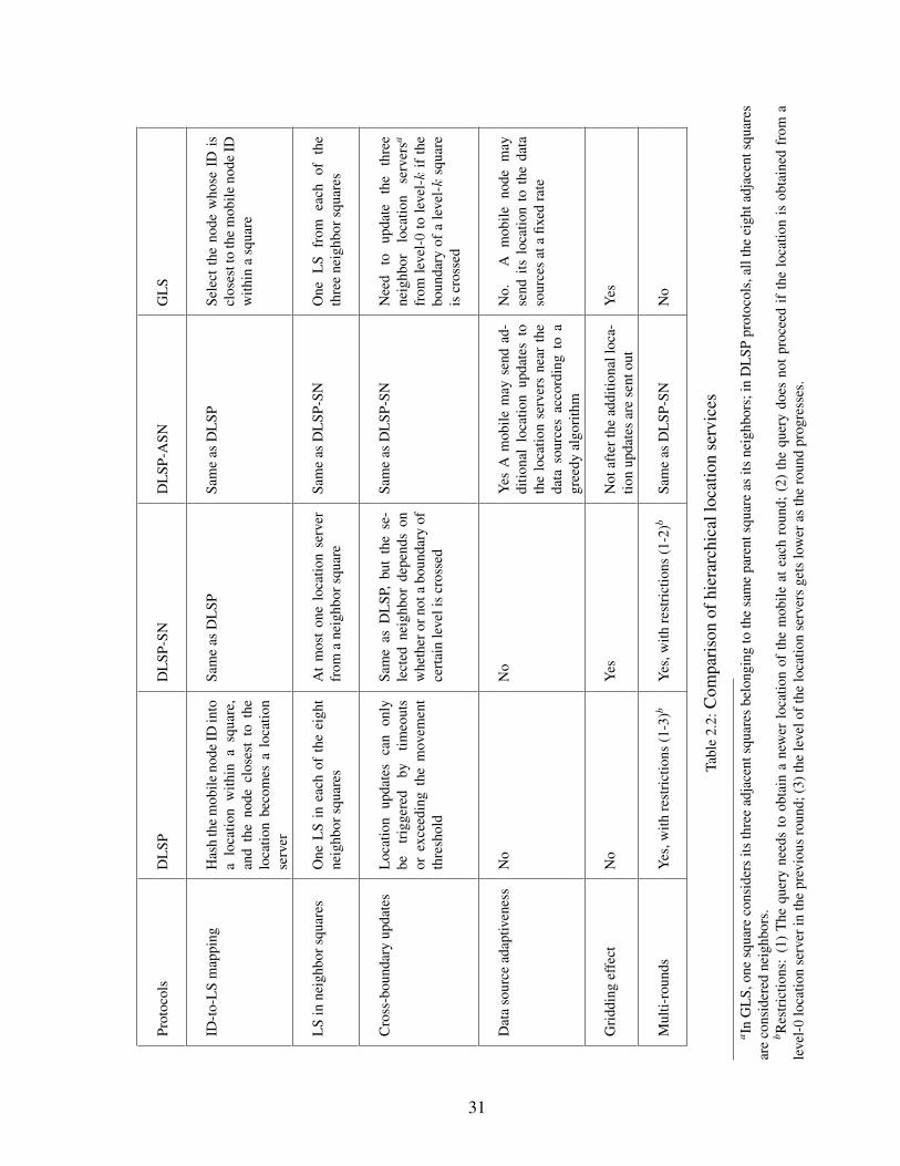
2.2 Comparison of hierarchical location services . . . . . . . . . . . . . . . . 31
2.3 Average per-hop latency of DLSP using S-MAC. The average per-hoplatency and its standard deviation vary with the network size. The move-ment thresholds can thus be derived from our analysis using Eq. 2.13 fordifferent network sizes. . . . . . . . . . . . . . . . . . . . . . . . . . . . 42
2.4 Average per-hop progress with varying numbers of nodes in 1600m×1600mnetworks. . . . . . . . . . . . . . . . . . . . . . . . . . . . . . . . . . . 48
3.1 The size of the area confined by the outer boundaries identified by TRA-VERSE when the standard deviation of the normal distribution for the lo-cation estimation errors vary. As the location estimation error increases,the size of the hole area is slightly decreased. . . . . . . . . . . . . . . . 77
3.2 The path lengths taken by GPSR and GFRHA, and their differences (%).Depending on the shape of the hole and the locations of sources and des-tinations, the performance gain (or loss) by GFRHA over GPSR signifi-cantly differs. . . . . . . . . . . . . . . . . . . . . . . . . . . . . . . . . 81
4.1 Notations used for ARCMA . . . . . . . . . . . . . . . . . . . . . . . . 95
x

ABSTRACT
EFFICIENT AND SECURE NETWORK SERVICES IN WIRELESSSENSOR NETWORKS
by
Min-gyu Cho
Chair: Kang G. Shin
Wireless sensor networks (WSNs) have been deployed for environment monitoring
and surveillance. A message delivery service is one of the most fundamental services for
WSNs, thus making its efficiency and effectiveness important. A widely-adopted protocol
for message delivery in WSNs is a geographic forward routing (GFR), in which messages
are greedily forwarded to their destinations. In this thesis, we develop network services
complementary to the existing GFR for efficient and secure message delivery in WSNs.
We first develop a distributed location service protocol (DLSP) for message delivery
to mobile nodes. Since GFR represents destinations of messages with destinations’ geo-
graphic locations, the knowledge of location of mobile nodes is necessary to ensure cor-
rect message delivery. In DLSP, mobile nodes select some sensor nodes as their location
servers, and publish the mobiles’ location information to the location servers. Sensor nodes
contact those location servers to retrieve the current location of mobile nodes when needed.
xi
DLSP provides systematic methods for mobile nodes to select location servers and publish
their location to those servers, and for sensor nodes to query mobiles’ location.
We then design an algorithm called TRAVERSE for hole boundary detection and ge-
ographic forward routing with hole avoidance (GFRHA) for efficient message routing.
TRAVERSE identifies boundaries of holes, i.e., areas without any functioning sensor node.
GFRHA then utilizes the identified hole information to route messages around holes while
being forwarded before they encounter holes. This way, the message path lengths, and
subsequently the message delay and energy consumption, can be significantly reduced,
depending on hole shapes and source and destination locations.
We also develop attack-resilient collaborative message authentication (ARCMA) for
message delivery. ARCMA is designed to tolerate node-capture attacks, in which attackers
obtain valid keys by compromising physically-exposed sensor nodes, and use the keys
to generate forged messages. To defend against such attacks, in ARCMA, messages are
collaboratively authenticated by a set of sensor nodes rather than by one node. The security
of ARCMA does not degrade unless attackers simultaneously compromise more than a
certain number of sensor nodes.
xii

CHAPTER I
INTRODUCTION
1.1 Overview of Wireless Sensor Networks
Wireless sensor networks (WSNs) have gained popularity since they are suitable for
numerous new applications. They are being adopted by various commercial, academic,
and military applications, such as healthcare systems, smart buildings, habitat monitoring,
fire detection and military surveillance.
WSNs are composed of a large number of sensor nodes and a relatively small number
of mobile nodes. Sensor nodes are used to monitor surrounding physical environments.
They are equipped with various sensors depending on the underlying application, such as
photometer, temperature sensor, and magnetometer. They also have a radio communication
module so that they can communicate with each other. However, to reduce the deployment
cost, they are typically stationary and resource-limited; they have limited memory and
processor capability, and they are battery-powered.
On the other hand, mobile nodes are carried by humans, or attached to manual or au-
tomated vehicles. They are used by human or automated users to interact with sensor
nodes. They usually have relatively abundant resources; they have more memory, more
CPU power, and faster and more stable wireless communication hardware. Also, they are
usually equipped with GPS-like devices to obtain their own geographic location.
In the typical application scenarios, sensor nodes are used to detect events of interest,
1
and mobile nodes are used to interact with sensor nodes to retrieve the information ac-
quired by sensor nodes. To detect the events of interest, sensor nodes are equipped with
adequate sensors. For example, temperature sensors and magnetometers are equipped for
fire detection and military surveillance applications, respectively. Sensor nodes often col-
laborate with other sensor nodes to improve the accuracy of detection. Mobile users such
as humans or automated vehicles use mobile nodes to query the events detected by sensor
nodes. These queries should be properly handled by sensor nodes.
To support these application scenarios, we need several network services. When an
event is identified by sensor nodes, we typically need to know the location and time of the
event. Thus, we need localization and synchronization services, which provide the location
estimation of sensor nodes and time synchronization among sensor nodes, respectively. As
in other networks, we also need a service to route messages to their destinations. We also
need a mechanism to process queries issued by mobile nodes.
In the rest of this chapter, we first describe existing network services in Section 1.2.
Then, we summarize our contributions with their motivations in Section 1.3, followed by
the overall architecture of sensor network applications with our contributions in Section 1.4.
Finally, this thesis is outlined in Section 1.5.
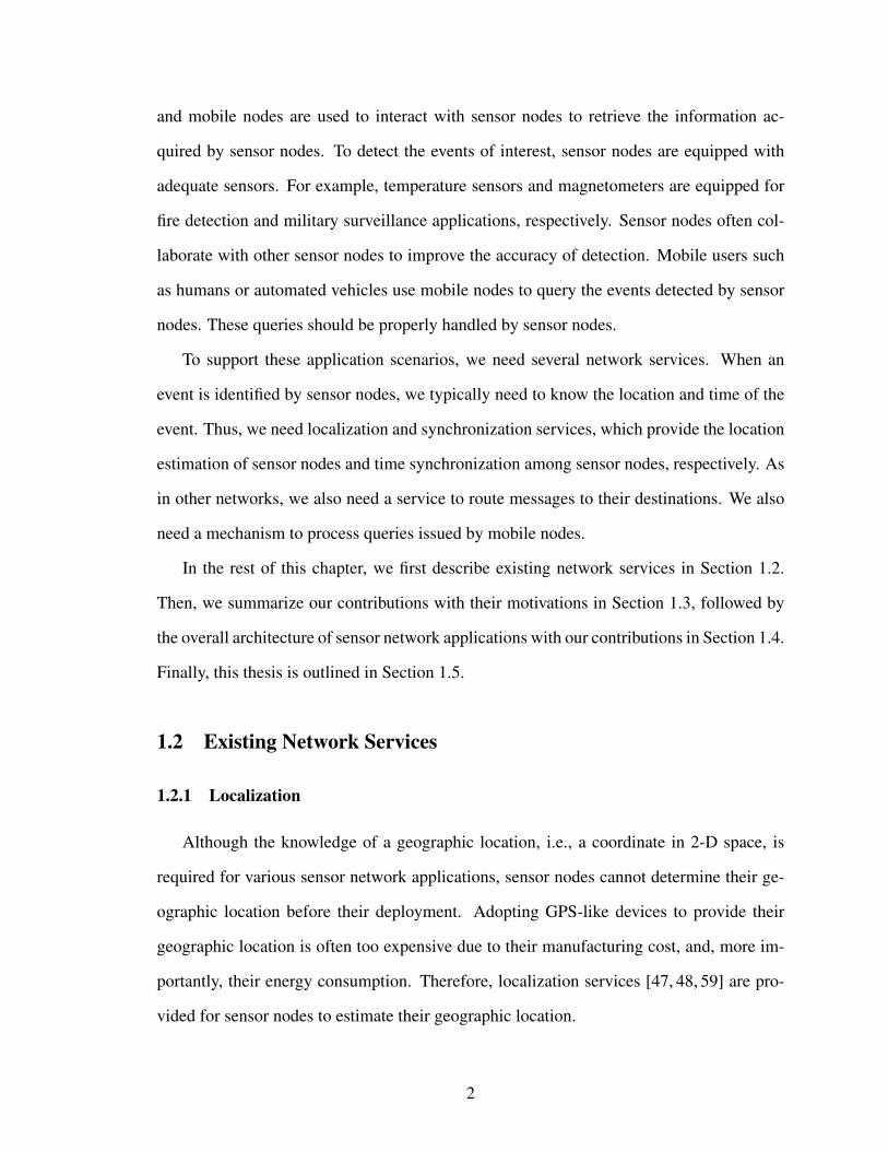
1.2 Existing Network Services
1.2.1 Localization
Although the knowledge of a geographic location, i.e., a coordinate in 2-D space, is
required for various sensor network applications, sensor nodes cannot determine their ge-
ographic location before their deployment. Adopting GPS-like devices to provide their
geographic location is often too expensive due to their manufacturing cost, and, more im-
portantly, their energy consumption. Therefore, localization services [47, 48, 59] are pro-
vided for sensor nodes to estimate their geographic location.
2
Most localization services estimate the geographic location of sensor nodes using two
phases: distance (or angle) estimation, and distance (or angle) combination. In the es-
timation phase, sensor nodes estimate the distance to (or angle with) other nodes in the
neighborhood, and in the combination phase, local estimations are combined to give the
global geographic location for every node in the WSN.
For the estimation phase, several techniques can be used to estimate the distance (or an-
gle) between a pair of nodes. The most popular techniques are received signal strength indi-
cator (RSSI), time of arrival (ToA), time difference of arrival (TDoA), and angle of arrival
(AoA). RSSI is measured by the communication circuit, and the measurement of received
signal strength is transformed into the distance between a pair of nodes. ToA and TDoA
are time-based measurement techniques, and they use the propagation delay as an estima-
tion of the distance between two nodes. TDoA uses two signals with different propagation
delays such as ultrasound or RF signals. AoA is measured by the directional antennas, and
such a measurement gives the relative direction (or angle) between two nodes.
In the combination phase, the global location of each sensor node is estimated by trian-
gulating the local estimations based on the aforementioned techniques. Several techniques,
such as convex optimization, multidimensional scaling (MDS), and quadrilaterals [48] have
been proposed to improve the efficiency or the accuracy of estimation.
Anchor nodes (or beacon nodes), which have exact geographic locations, are often used
for the combination phase to reduce the overhead or increase the accuracy of estimation.
A small portion of sensor nodes can be used as anchor nodes; they obtain their geographic
locations through GPS-like devices or by manual measurement of their locations.
Even though some localization services [47, 48] do not require anchor nodes, the an-
chor nodes may be necessary to transform the coordinates used by localization services to
common reference coordinates. When no anchor node is used, the estimation results of lo-
calization services can be realized in a Euclidean space only up to isometry (in the case of
distance estimation) or conformal transformation (in the case of angle estimation). Thus, a
3
small number of anchor nodes are necessary if we want to transform the coordinate system
used by the localization service to the reference coordinate system.
After completing the two processes of localization services, each sensor node knows its
geographic location. We can also broadcast the coordinates of nodes that have the minimum
and the maximum value for x- or y-coordinates to inform sensor nodes the deployment area
boundary.
In this thesis, we adopt localization services [47, 48] which do not require any special
hardware such as GPS-like devices or directional antennas. Without any GPS-like devices,
sensor nodes can use any of the aforementioned localization services to estimate their geo-
graphic location. We may need to load geographic location information to a small number
of sensor nodes that are used as anchor nodes. Alternatively, we may use a small number
of mobile nodes equipped with GPS-like devices to emulate anchor nodes. Throughout
this thesis, we assume that sensor nodes know their geographic location and the size of
deployment area from a localization service.
1.2.2 Geographic forward routing
Geographic forward routing (GFR) protocols [7, 33, 39] have been widely adopted by
various sensor network applications because of their low resource requirements. In GFR,
sensor nodes are assumed to know their geographic location, and the destination of a mes-
sage is specified with a geographic “location” instead of another network identifier such
as an IP address or a node ID. As most sensor network applications require sensor nodes
to know their geographic location through a localization service, GFR adds little commu-
nication and memory overhead to maintain routing information; GFR only requires sensor
nodes to have their own and their immediate neighbors’ geographic location.
GFR greedily forwards messages using only locations of immediate neighbors. In GFR,
a forwarding node selects the next hop closer to the destination than itself. Typically, the
node closest to the destination would be selected as the next hop. Then, the message will
4
be forwarded towards the destination at each hop, and eventually it will be delivered to
the destination location. When the message is delivered to the destination location, a node
closest to the destination location will process it.
However, a forwarding node may not have any neighbor node closer to the destination
than itself if there is a hole (or a void area) on the network. A hole can be viewed as an area
without any functioning sensor node. When a hole is encountered, GFR should invoke a
mechanism to route the message around the hole. For example, GPSR [33], a well-known
GFR protocol, starts perimeter forwarding, in which a message is forwarded around the
perimeter of the hole using the right-hand rule. This forwarding mode is expensive because
a path taken by this mode can be much longer than the shortest path to the destination.
1.2.3 Data-Centric Storage
Data-centric storage (DCS) [24,27,42,56] provides in-network storage and query mech-
anisms for sensor networks. In DCS, events identified by sensor nodes are stored at the
sensor nodes, called storage nodes, at the predestined locations by their event types. The
information about identified events is forwarded to the storage nodes, and queries issued by
(typically, mobile) users are forwarded to, and processed at, the storage nodes. Different
types of events will be stored at different storage nodes for load-balancing and reliability.
DCS was initially proposed in [56], where a geographic hash table (GHT) is used to
determine the location of storage nodes. In a GHT, sensor nodes are required to know their
geographic locations and route messages using GFR. In a GHT, the locations of storage
nodes are determined by common hash functions shared by all nodes. The hash function
takes the event type as an input, and generates geographic locations to determine location
of storage nodes for the given type of events. Several improvements for DCS have been
proposed to enhance the performance of GHT [24, 27, 42].
5

1.2.4 Time Synchronization
Time synchronization among sensor nodes is required for numerous sensor network
applications and security protocols. Sensor network applications require knowledge of
the time of the event identification. Also, many security protocols require (loose) time
synchronization to prevent replay, or other attacks.
Synchronization services continuously adjust the clocks of sensor nodes to achieve
global synchronization by compensating for the time differences caused by different clock
drift rates of sensor nodes. Synchronization services typically adjust the clocks of nodes
in the neighborhood and propagate the adjustment as necessary to achieve global synchro-
nization.
Several time-synchronization protocols [16, 22, 63, 64] have been proposed for WSNs.
These services can be categorized by the type of messages exchanged for local clock ad-
justments, and the existence/absence of master nodes whose clocks are used as reference
clocks [77].
1.3 Motivation and Contributions
1.3.1 Distributed Location Service Protocol
Geographic forward routing (GFR) protocols are widely used for WSNs since they
are well-suited for the requirements of WSN applications. Since a geographic location is
specified as a destination in GFR, delivering messages to mobile nodes is difficult since
their locations are not fixed. When sensor nodes need to send messages to a certain mobile
node, they may not have the mobile’s current location. Therefore, we need a network
service to provide the geographic location of mobile nodes to enable message delivery
using GFR.
In this thesis, we develop a distributed location service protocol (DLSP) to provide the
current location of the mobile users. Using DLSP, sensor nodes can retrieve the current
6
location of mobile nodes, so as to send messages to mobile nodes using GFRs. We assume
that mobile nodes obtain their geographic location by GPS-like devices, while sensor nodes
do so by a localization service.
In DLSP, each mobile node publishes its location information to some sensor nodes,
called location servers, and sensor nodes access those location servers to retrieve the mo-
biles’ location information when necessary. DLSP provides systematic methods to select
location servers, publish mobile nodes’ location, and query location information based on
a hierarchical grid structure. Specifically, we design DLSP and propose the optimizations
of DLSP, and evaluate them with mathematical analysis and extensive simulation.
1.3.2 Distributed Hole Detection
The deployment areas of WSNs may contain holes, which are the areas without any
functioning sensor node. Holes are formed by obstacles in the battery-deployment areas,
the depleted or faulty nodes, or active attacks of malicious users.
Detecting holes in WSNs is important for network management. With the hole infor-
mation, one can determine the terrain of the deployment area or the active events, such as
an attack. We can also use the hole information to improve the performance of network
protocols on WSNs. For example, we can use the information to route messages around
holes to avoid the use of expensive detouring mechanisms in GFR.
We develop an algorithm, called TRAVERSE, to detect hole boundaries. After deploying
a sensor network, TRAVERSE is invoked to locate holes on the WSN. TRAVERSE is a
distributed algorithm, and has only nodes around the possible holes participate in the hole
detection process. The algorithm is also invoked upon detection of a topology change.
We also propose geographic forward routing with hole avoidance (GFRHA) to route
messages around the detected holes. In GFRHA, the identified hole information is dissem-
inated to sensor nodes near the detected holes. GFRHA utilizes this information to route
messages around the holes without invoking any expensive detouring mechanism. By de-
7
touring messages around holes, the path length is shortened, reducing the delay and the
energy consumption for message delivery.
1.3.3 Attack-Resilient Collaborative Message Authentication
Sensor networks are often used for collecting critical information. However, secur-
ing sensor networks is very difficult, especially because sensor nodes are often physically
exposed to attackers. In WSNs, attackers can launch node-capture attacks in which the at-
tackers physically access and compromise sensor nodes. After compromising sensor nodes,
the attackers may retrieve all the information stored in the sensor nodes including keying
materials. We cannot afford expensive hardware-based solutions for sensor nodes since we
usually need to deploy a large number of sensor nodes.
We design a security mechanism by focusing on authenticated message delivery for
DCS under node-capture attacks. In DCS, as in other sensor network applications, au-
thenticated message delivery is very important to prevent attackers from inserting, modify-
ing, and accessing information. We achieve authenticated message delivery by proposing
attack-resilient collaborative message authentication (ARCMA).
In ARCMA, a message is collaboratively authenticated by a set of sensor nodes. More
specifically, a message is authenticated by k nodes instead of a single sensor node, where
k is a user-defined parameter. For this, we require dense deployment of sensor nodes such
that any event can be detected by k or more nodes. With ARCMA, we can prevent the
insertion or modification of fakes messages. Thus, we can prevent attackers from reporting
false data to storage nodes, issuing queries, and responding to queries with false data. The
security of ARCMA is not degraded if less than k nodes are compromised.
1.4 Architecture of Sensor Network Applications
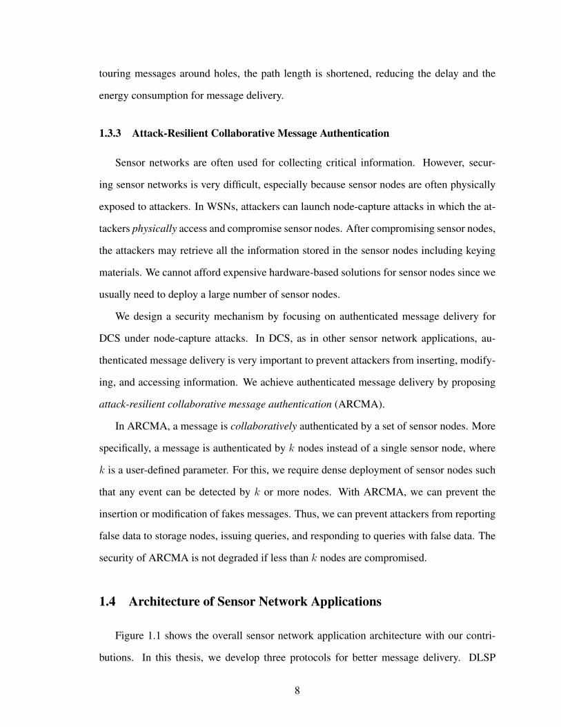
Figure 1.1 shows the overall sensor network application architecture with our contri-
butions. In this thesis, we develop three protocols for better message delivery. DLSP
8
!"
#$%$"&'(%)*+",%-)$.'"/#&,0"1223*+$4-("
5$6*-7",'(8-)87"&3-+97":",'(8-)8"
;'%<-)9"
,')=*+'8"
5->4(."
,')=*+'"
,'+>)*%?"
,')=*+'"
,>22-)4(."
,')=*+'8"
#@,A" 15&B1"#C#"
DE5" @-+$3*F$4-("
G*H'",?(+I"
Figure 1.1: The architecture of sensor network applications with our contributions
enables message delivery to mobile nodes using GFR, DHD provides the hole information
and improves the performance of GFR in the presence of holes, and ARCMA provides the
authenticated message delivery in WSN.
1.5 Outline
The rest of this thesis is organized as follows. Chapter II presents the distributed loca-
tion service protocol (DLSP) to provide the location of mobile nodes for message delivery
to mobile nodes with geographic forward routing. Chapter III presents a distributed hole
detection algorithm, called TRAVERSE, which identifies the boundaries of holes in a WSN,
and geographic forward routing with hole avoidance (GFRHA), which uses the identified
hole information to route messages around holes. Chapter IV describes attack-resilient col-
laborative message authentication (ACRMA), which supports authenticated message de-
livery in WSNs. ARCMA can tolerate node-capture attacks. Chapter V concludes this
9

thesis.
10
CHAPTER II
DISTRIBUTED LOCATION SERVICE PROTOCOL
2.1 Introduction
Many sensor network applications, such as habitat monitoring [45], emergency res-
cue, battlefield surveillance, and border monitoring [51, 77] require interaction between
stationary sensor nodes and mobile nodes. That is, a large number of resource-limited
sensor nodes are deployed in a certain geographical area for physical-environment moni-
toring, and some mobile nodes may move around the area and receive event notifications
from the stationary sensors. For example, in the emergency-rescue or military applications,
emergency rescuers/vehicles or soldiers/military vehicles, as mobile nodes, need to rescue
missing people or track enemies. In these applications, mobile nodes interact with sen-
sor nodes to retrieve mission-related information such as the location of missing people or
enemies.
To support the aforementioned applications, we need to provide a routing mechanism
to forward information about the events detected by sensor nodes to mobile nodes. This
information routing/forwarding should be done by sensor nodes since mobiles may not
always form a connected network depending on their density and movement, although
mobiles often have a longer radio communication range than sensor nodes. To meet the
application requirements, the routing mechanism should perform well for a wide range
of the mobiles’ speed and movement pattern. Depending on their mission and resources,
11

mobile nodes may travel with varying speeds to arbitrary locations in the network. For
example, foot soldiers or emergency-rescuers may move at a low speed while ambulances,
fire trucks, or military vehicles may move at a high speed to reach the missing people, or
detect enemies.
2.1.1 Background
There are two types of approaches to routing sensed data to a mobile node: (1) TTDD [72],
Bread Crumb Routing [69], and Last Encounter Routing (LER) [28] that do not require
knowledge of the mobile’s whereabout, and (2) Geographic Forward Routing (GFR) [33,
39], Landmark Routing [65], and Beacon Vector Routing (BVR) [20] that require knowl-
edge of the mobile’s location.
In (1), TTDD allows data sources (i.e., sensors) to proactively build grid structures
over the entire network to disseminate the sensed data, so the overhead of publishing data
may be amortized when there are many mobile nodes. Bread Crumb Routing assumes a
mobility model under the constraint that the sensors marked by the mobile node must form a
connected path. However, in the above-mentioned scenarios, this path may be disconnected
because (i) the mobile fails to leave marks on sensors as a result of message loss; (ii) the
path may run through a deployment hole, and thus, the sensor marked by the mobile cannot
communicate directly with any of previously-marked sensors; (iii) a sensor node on the path
may fail or be destroyed. In LER, each node keeps the database of the location and time
of other nodes it has directly communicated with, and uses the database to route packets
using the updated location information as packets are being routed to the destination. This
routing scheme becomes very similar to Bread Crumb Routing in our application scenario,
where sensor nodes are stationary. Thus, LER shares the same problems with Bread Crumb
Routing.
In (2), the mobile needs to periodically report its geographic location or virtual address
to selected nodes, called location servers, in order to use GFR, Landmark Routing, or
12

BVR. Other nodes can acquire the mobile’s location from one of its location servers and
then deliver data to the mobile node using one of these routing protocols.
A number of location-service protocols have been proposed for mobile ad hoc networks
(MANETs) to be used with GFR. GHLS [12], Twins [66], and Home-Zone-Based Location
Service all use hash functions to select a centralized location server. That is, they select only
one location server for a given mobile node. Particularly, GHLS hashes the mobile node’s
ID into a geographic location, and the node closest to that location serves as the central
location server for the mobile. In these protocols, location queries are forwarded to and
processed by the centralized location server.
XYLS [62] lets the mobile node select a thick column of nodes as its location servers.
In XYLS, a mobile node updates nodes in the same column, i.e., nodes whose x-coordinate
is within a certain range of the mobile node. Queries are forwarded in the same row, i.e., in
the parallel direction of the x-axis until they reach location servers.
GLS [40], DLM [70], HLS [34], and MLS [19] are hierarchical location service pro-
tocols, i.e., the mobile node constructs a hierarchy of location servers over a grid struc-
ture. In these protocols, mobile nodes send their location to location servers, and location
queries are forwarded to and processed by those location servers. Beacon Location Service
(BLS) [52] is developed for the location service for BVR, in which routing is based on a
beacon-vector, i.e., a vector of hop-distance to beacon nodes, instead of geographic location
as in GFR. Also, Landmark Routing [65] provides a hierarchical lookup service to provide
a mapping between the node ID and the landmark address. The hierarchical lookup mech-
anisms provided by these protocols are similar, but they are tailored differently by different
designs of location update and query mechanisms. Note that BVR and landmark routing
need a separate service to map a specific location to beacon-vector or landmark address if
we want to send a packet to the location, which is often required in a WSN. Also, landmark
routing is not scalable since the discovery of landmarks are based on the distance-vector
routing; additional route-discovery packets should be exchanged. In GFR-based location
13

services, such landmark discovery is not necessary since location servers are selected at the
pre-defined geographic locations.
These location service protocols, however, are not applicable to sensor networks due
to the usually high per-hop latency in a sensor network which ranges from a few hundred
milliseconds to a few seconds [43, 75], while that of a MANET is an order-of-magnitude
lower (tens of ms) [26,35]. The high per-hop latency in a sensor network can be attributed
to scheduling delay and transmission time. First, wireless communication consumes much
more energy than other operations for (severely energy-constrained) sensor nodes. Hence,
energy-efficient MAC protocols avoid idle listening and overhearing by scheduling trans-
mission and listening periods (e.g., S-MAC [76] and T-MAC [11]), or low-power channel
polling (e.g., WiseMAC [15] and BMAC [54]), or both (e.g., SCP [75]). As a result, the
radio’s duty cycle can be limited to a few percentages. Thus, a packet has to be held for a
certain period of time before taking its next hop. Second, a sensor node’s radio usually has
a lower bandwidth, incurring a longer transmission time. For example, Mica2 (MicaZ) has
a bandwidth of 19.5 kbps (250 kbps), while MANETs typically use wireless LAN cards of
11 Mbps or 54 Mbps.
This high per-hop latency makes packet transmission in a sensor network much slower
than in a MANET. Moreover, a sensor network is usually of much larger scale than a
MANET. Therefore, the location-service protocols intended for MANETs are unlikely to
perform well in sensor networks, because, while a message is being delivered from its
source to a location server, then to the mobile receiver’s location obtained from the location
server, the mobile could have moved too far away to receive the message directly as in
GHLS or even by using forward pointers as in GLS. This problem becomes more evident
as the mobile moves faster.
14

2.1.2 Proposed Approach
In this chapter we present a distributed location service protocol (DLSP) for a hybrid
wireless network of stationary sensors and mobile nodes. DLSP is built on a hierarchical
grid structure. A mobile selects multiple location servers at each level of the hierarchy,
and sends location updates more frequently to the lower-level location servers than to the
higher-level ones. A location query (that also contains a data packet to be delivered) may
take multiple rounds of “lookup-and-chase” to reach the mobile receiver.
Through a rigorous analysis, we derive the condition under which a high query-delivery
ratio (i.e., the data-delivery success rate in DLSP) is achieved, and show how to configure
the protocol parameters to ensure the scalability of the location service. Here ‘scalability’
means that, as the network size increases, the location service protocol preserves the high
query-delivery ratio and the protocol overhead is proportional to O(log(N)), where N is
the network size. We find that, in order to preserve a high query-delivery ratio, the mobile’s
speed should be below a certain fraction of the packet-transmission speed, which depends
on the underlying movement threshold. For example, if the movement threshold for the
lowest-level location servers is the same as the node’s radio range, the mobile’s speed
limit is one-tenth of the packet-transmission speed. The theoretical speed limit is a one-
fifth of the packet-transmission speed beyond which DLSP does not scale regardless of the
movement threshold.
DLSP incurs a high location-update overhead because a mobile needs to update multi-
ple location servers at each level with its location information. To alleviate this problem,
we propose an optimization, called DLSP with a Selected Neighbor (DLSP-SN), in which
the mobile updates the location server in at most one neighbor square at each level. A
neighbor square is selected based on the mobile’s trajectory. DLSP-SN achieves a signif-
icant reduction of update overhead. However, due to the gridding effect,1 DLSP-SN may
1‘Gridding effect’ means that the source and destination nodes across but close to the boundary of a high-level square may require the query to travel many hops upward (in the hierarchy) to the common (parent)square containing both nodes. Both GLS and DLSP-SN suffer from the gridding effect, but DLSP does not.
15

incur more rounds of lookup-and-chase than DLSP, thus making the average path length
of location queries greater than that of DLSP and increasing data-delivery cost. In order
to make a tradeoff between location-update and data-delivery costs, we present a greedy
adaptation mechanism, called DLSP-ASN, to improve the overall energy-efficiency.
The contributions of this work are summarized as follows.
• Design of DLSP: We design a novel hierarchical location service. In DLSP, location-
updates are published to hierarchical location servers, and location-queries are pro-
cessed recursively using these hierarchical location servers. DLSP can efficiently
provide mobiles’ location information with a wide range of mobiles’ speeds even in
the presence of sensor node failures.
• Optimization of DLSP: We provide two optimized algorithms for DLSP, DLSP-
SN and DLSP-ASN. The former focuses on reducing the location-update overhead,
while the latter makes a good balance between the location-update overhead and the
data-delivery ratio.
• Evaluation of DLSP: We rigorously and throughly evaluate DLSP and its optimiza-
tions. First, we derive the condition under which DLSP guarantees a high data-
delivery ratio using a mathematical analysis. Second, we extensively simulate DLSP
with various scenarios and parameters to show its performance in diverse environ-
ments.
The rest of this chapter is organized as follows. Section 2.2 describes the details of
DLSP. Section 2.3 derives the condition for DLSP to achieve a high packet-delivery ra-
tio, while Section 2.4 analyzes the overhead of DLSP, and presents an enhanced version
of DLSP, called DLSP-SN. Section 2.5 proposes a greedy adaptation mechanism, DLSP-
ASN. In Section 2.6 we use simulation to evaluate the performance of location services.
We conclude the chapter and discuss future directions in Section 2.7.
16

P (S),P (R, T )
Location of a stationary sensor node S, or of a mobile node R at time T
Sk,j(S),Sk,j(R, T )
Sk,0(S) is the level-k square the sensor S resides, and Sk,j(S) (j = 1, · · · , 8) are theeight level-k neighbor squares adjacent to Sk,0(S). Sk,j(R, T ) is the level-k square themobile R resides at time T , and Sk,j(R, T ) (j = 1, · · · , 8) are the level-k neighborsquares
LSRk,j(S),
LSRk,j(R, T )
R’s level-k location server in the square Sk,j(S), or Sk,j(R, T )
ALSRk (S) R’s adaptive location server for a data source S in the square Sk,0(S)
L Edge length of the square field of interesth Level of the largest square, i.e., the entire deployment field` Edge length of a level-0 squarem Movement threshold for level-0 location servers 2−m`
τ Time threshold for location updates at level-0 location serversth Average per-hop latency, including transmission/retransmission time, and scheduling
delayp Average per-hop progress, or decrease of Euclidean distance to the destination for each
hop takenr Radio rangev Mobiles’ average speeddist(P1, P2) Distance between two locations, P1 and P2
Table 2.1: List of symbols
2.2 Distributed Location Service Protocol
We now present the details of DLSP. We assume that a large number of stationary
sensors have been placed randomly and uniformly in a field of interest and a relatively
smaller number of mobile nodes move around within the field. Geographic routing (e.g.,
GPSR [33]) is used for multi-hop routing. Each sensor node can determine its location by
using a localization service [31, 59]. Likewise, each mobile either is equipped with a GPS
receiver or can estimate its location using the neighbor sensors’ location information.
Table 2.1 lists the notation used in this chapter.
2.2.1 Selection and Update of Location Servers
A sensor network is assumed to have been deployed in a square field as in GHT [56].
Similar to GLS [40], the entire square field is partitioned into a grid as shown in Figure 2.1.
17
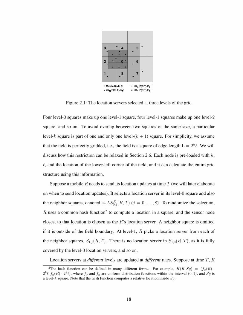
Figure 2.1: The location servers selected at three levels of the grid
Four level-0 squares make up one level-1 square, four level-1 squares make up one level-2
square, and so on. To avoid overlap between two squares of the same size, a particular
level-k square is part of one and only one level-(k + 1) square. For simplicity, we assume
that the field is perfectly gridded, i.e., the field is a square of edge length L = 2h`. We will
discuss how this restriction can be relaxed in Section 2.6. Each node is pre-loaded with h,
`, and the location of the lower-left corner of the field, and it can calculate the entire grid
structure using this information.
Suppose a mobileR needs to send its location updates at time T (we will later elaborate
on when to send location updates). It selects a location server in its level-0 square and also
the neighbor squares, denoted as LSR0,j(R, T ) (j = 0, . . . , 8). To randomize the selection,
R uses a common hash function2 to compute a location in a square, and the sensor node
closest to that location is chosen as the R’s location server. A neighbor square is omitted
if it is outside of the field boundary. At level-1, R picks a location server from each of
the neighbor squares, S1,j(R, T ). There is no location server in S1,0(R, T ), as it is fully
covered by the level-0 location servers, and so on.
Location servers at different levels are updated at different rates. Suppose at time T , R
2The hash function can be defined in many different forms. For example, H(R,Sq) = (fx(R) ·2k`, fy(R) · 2k`), where fx and fy are uniform distribution functions within the interval (0, 1), and Sq isa level-k square. Note that the hash function computes a relative location inside Sq.
18

R
S
P(R,T1)
LS0,0(R,S)
LS1,0(R,S)
LS2,0(R,S)
)1TP(R,
)2TP(R,
S
R
A
LS1,0(R,A)
LS0,0(R,A)
Figure 2.2: Round 1 of location query pro-cessing
Figure 2.3: In round 2, only the locationserver in the shaded level-1 neighbor squareis visited
has sent a location update (i.e., P (R, T )) to level-k location servers. It will then send the
next update to the level-k servers at T+∆T if and only if dist(P (R, T ), P (R, T+∆T )) ≥
2k−m` (i.e., the movement threshold) or ∆T ≥ 2kτ (i.e., the timeout). R sets the lifetime
of its location servers to be slightly larger than 2 · ∆T , where ∆T = min(2kτ, 2k−m`v
), to
tolerate a loss of location update or jitter. If a location server does not receive a new update
from the mobile R before this lifetime expires, it is no longer a location server for R.
Selection of location servers in all neighbor squares ensures the availability of a level-k
location server if the distance to the mobile node is within 2k`, and thus, prevents a gridding
effect. Also, the hash function lets different mobile actors choose different sensor nodes as
their location servers. As a result, the protocol evenly distributes the workload and energy
consumption among the sensor nodes.
2.2.2 Processing of Location Queries
When a sensor node S sends a data message to R, it only knows R’s ID. First, it tries
to find R’s location from its neighbor’s table and local location cache (i.e., it is a location
server for R). If R’s location is not found, S encapsulates the data into a location query,
and sends it to a location server. Once R’s location is found, the data message is sent to
19

that location using geographic-location-based-routing. This lookup-and-chase process is
illustrated by an example in Figures 2.2 and 2.3.
In Figure 2.2, S first assumes that R has visited somewhere nearby — R and S are in
the same level-0 square or two adjacent level-0 squares. Formally, S assumes LSR0,j(R, T )
to be LSR0,0(S). So, the location query is sent to LSR0,0(S). However, LSR0,0(S) does not
have R’s location information, so it tries to find R’s location in a larger square by sending
the query to LSR1,0(S), and so on. Eventually, LSR2,0(S) has R’s location information at
time T1 (i.e. LSR2,0(S) is also LSR2,4(R, T1)) , denoted as P (R, T1), so it sends the query to
P (R, T1). This process of looking for the location of, and chasing, the mobile is called a
round.
If R moves fast and if S and R are far apart, by the time the location query reaches the
location P (R, T1), R could have moved too far away from P (R, T1) to receive the location
query. In such a case, the query will be received by the node A closest to P (R, T1). Unlike
GLS, A does not maintain any forwarding pointer3 under DLSP. Instead, it starts a new
round. As shown in Figure 2.3, the query first goes to LSR0,0(R,A), then to LSR1,0(R,A)
(i.e., LSR1,6(R, T2)), which has more recentR’s location information, P (R, T2). Finally, the
query catches up with R near P (R, T2).
After receiving the query, R may decide whether or not to send its location information
to S, which caches the location for later queries. Such a decision should depend on the
sender’s transmission rate, as discussed in Section 2.5.
2.3 Conditions for High Packet-Delivery Ratio
In this section, we first derive the condition for achieving a high packet-delivery ratio
under DLSP. Then, we discuss how to configure the parameters of DLSP to make it scal-
able. DLSP is found to be scalable if the mobile’s speed is lower than a certain fraction of
3In GLS, a mobile leaves a forwarding pointer in the lowest-level grid from which it moves out, so that aquery may follow the mobile using the forwarding pointers.
20

Time at
Location
Update
Location
Query
Location
Query
)1T P(R,
Time at
2T
1T
T!
4T
3T
0t
LS0,j(R,T1)
Figure 2.4: The timeline of events for location query processing at level-0.
the packet-transmission speed, which depends on the movement threshold used. Finally,
we present the condition for achieving a high packet-delivery ratio in GHLS, and also show
that GHLS is not scalable.
2.3.1 Conditions for High Packet-Delivery Ratio under DLSP
Our analysis of DLSP consists of the base case and the inductive step. The base case
analyzes how a location query can catch up with the mobile receiver after obtaining its
location information from a level-0 location server. The inductive step analyzes how the
location query can get closer to the mobile by completing each round.4
2.3.1.1 The Base Case
Suppose, at time T1,R sends its location, P (R, T1), to a level-0 location server, LSR0,j(R, T1),
j ∈ {0, 1, . . . , 8}. The location server receives the location update at time T3. At time T4, it
receives a location query and forwards the query to P (R, T1). The location query reaches
location P (R, T1) at time T2. The timeline of these events are shown in Figure 2.4.
In order to have R receive the query at T2, the following condition must be satisfied:
dist(P (R, T1), P (R, T2)) ≤ r. (2.1)
Suppose ∆T = T2 − T1, then dist(P (R, T1), P (R, T2)) is bounded by ∆T v, because
4The analysis of DLSP was coworked with Zhigang Chen and published in [10]. For the completeness ofthe thesis, the analysis is presented here.
21

the distance is maximized whenRmoves on a straight line between T1 and T2. The average
speed is computed as the length of the trajectory curve between T1 and T2 over ∆T . ∆T
can be broken into three components, T3 − T1, T4 − T3, and T2 − T4. T3 − T1 denotes the
average latency of the location update from P (R, T1) to LSR0,j(R, T1); T4 − T3 represents
the average obsoleteness of the location information at the location server; T2−T4 denotes
the average latency of the location query from LSR0,j(R, T1) to P (R, T1).
Let d0 be dist(P (R, T1), L0,j(R, T1)), the average distance between R and a level-0
location. Then, considering R as a random point in an `× ` square, and the location server
as a random point in the same square or one of the eight adjacent squares, we get d0 ≈ 1.27`
according to a numerical analysis. Also, we let t0 be the update interval for level-0 location
servers. We have T3−T1 = T2−T4 = d0pth, and T4−T3 = 1
2t0 because T4 ranges from T3
to T3 + t0. So,
∆T =1
2t0 + 2
d0
pth. (2.2)
Also, from Section 2.2, we have
t0 =
τ if v < 2−m`τ
2−m`v
if v ≥ 2−m`τ
.(2.3)
From Eq. (2.3), we have
vt0 ≤ 2−m`. (2.4)
Therefore,
dist(P (R, T1), P (R, T2)) ≤ 1
2t0v + 2
d0
pthv (2.5)
22
In order to satisfy Eq. (2.1), we simply let 12t0v + 2d0
pthv ≤ r. That is,
τ v + 5.08`pthv ≤ 2r if v < 2−m`
τ
2−m`+ 5.08`pthv ≤ 2r if v ≥ 2−m`
τ.
(2.6)
Approximately, Eq. (2.6) can be satisfied if
2−m`+5`
pthv ≤ 2r. (2.7)
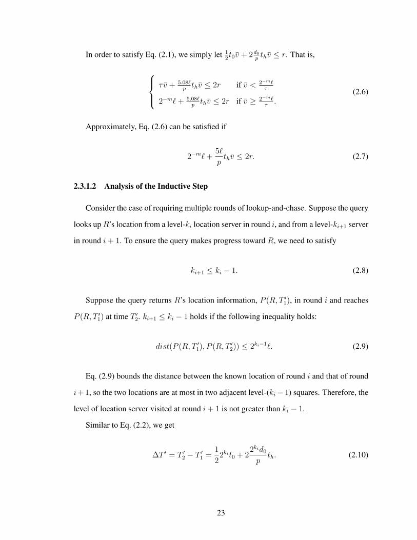
2.3.1.2 Analysis of the Inductive Step
Consider the case of requiring multiple rounds of lookup-and-chase. Suppose the query
looks upR’s location from a level-ki location server in round i, and from a level-ki+1 server
in round i+ 1. To ensure the query makes progress toward R, we need to satisfy
ki+1 ≤ ki − 1. (2.8)
Suppose the query returns R’s location information, P (R, T ′1), in round i and reaches
P (R, T ′1) at time T ′2. ki+1 ≤ ki − 1 holds if the following inequality holds:
dist(P (R, T ′1), P (R, T ′2)) ≤ 2ki−1`. (2.9)
Eq. (2.9) bounds the distance between the known location of round i and that of round
i+ 1, so the two locations are at most in two adjacent level-(ki− 1) squares. Therefore, the
level of location server visited at round i+ 1 is not greater than ki − 1.
Similar to Eq. (2.2), we get
∆T ′ = T ′2 − T ′1 =1
22kit0 + 2
2kid0
pth. (2.10)
23

So, we have
dist(P (R, T ′1), P (R, T ′1)) ≤ 1
22kit0v + 2
2kid0
pthv (2.11)
In order to satisfy Eq. (2.8), we simply let 122kit0v + 22kid0
pthv ≤ 2ki−1`. That is,
τ v + 5.08`pthv ≤ ` if v < 2−m`
τ
2−m`+ 5.08`pthv ≤ ` if v ≥ 2−m`
τ.
(2.12)
Again, due to Eq. (2.4), Eq. (2.12) can be satisfied if
2−m`+5`
pthv ≤ `. (2.13)
2.3.2 Configuration of Protocol Parameters for DLSP
The above analysis provides insights into which parameters affect the packet-delivery
ratio and how they can be configured to achieve the scalability of DLSP with respect to
query delivery.
2.3.2.1 Configuration of `
Consider the condition of the base case, Eq. (2.7), and that of the inductive step,
Eq. (2.13). The condition of the base case is stronger than that of the inductive step if
` ≥ 2r. Moreover, both Eqs. (2.7) and (2.13) are independent of the field edge length, L.
Therefore, as long as data can be delivered within a small region (level-0 squares) of edge
length ` ≥ 2r, it can be delivered from an arbitrarily far away node. In fact, we need
` = 2r (2.14)
because the overhead of location updates increases as ` increases (in Section 2.4).
24

2.3.2.2 Configuration of m
In Eq. (2.7), 5`pthv is always positive since th is not negligible. So, m must be a positive
integer. Again, the overhead of location updates is proportional to 2m when the mobile’s
speed is above the threshold. Therefore, m should be set to 1, and the movement threshold
is r.
2.3.2.3 Mobile’s Speed Limit
From Eq. (2.7), if m = 1, v < r5`
pth
= p10th
, which is a one-tenth of the packet-
transmission speed. If the movement threshold for location updates gets smaller, the loca-
tion updates become more frequent, and the mobile is allowed to move faster. However,
v < 2r5`
pth
must always hold, and the speed can never be greater than p5th
. So, the mo-
bile’s theoretic speed limit is a one-fifth of the packet transmission speed, no matter how
frequently the location servers are updated.
2.3.3 Choice of Design Paradigm
GHLS (i.e., a centralized paradigm) can be considered as a trivial case of DLSP (i.e., a
hierarchical paradigm), in which ` = L. The analysis of GHLS is the same as that of the
base case in DLSP, except that d0 ≈ 0.5L because the mobile and its location server are
considered two random points in the L× L square.
Suppose the movement threshold for updating the location server is vt0 ≤ d. We need
to satisfy
d+2L
pthv ≤ 2r. (2.15)
When th is not very small, Eq. (2.15) may not hold for large networks and fast mobiles.
Based on Eqs. (2.15), (2.4), and (2.14), we can conclude that, regardless of the mobile’s
speed, the conditions of GHLS (i.e., the centralized paradigm) are stronger than those of
25

the hierarchical paradigm if L < 2.5l. So, the centralized paradigm is favorable for low
mobile’s speed, very low per-hop packet latency, or small/ median networks because of its
simplicity and lower overhead [12]. For large networks with high mobility and non-trivial
packet latency, the hierarchical paradigm should be used.
2.4 Analysis of Location-Service Overhead
In this section, we first analyze the overhead of location updates under DLSP and then
propose a design optimization, called DLSP with a Selected Neighbor (DLSP-SN), which
significantly reduces the location-update overhead.
2.4.1 Analysis of Location-Update Overhead
Let U denote the total overhead of location updates, and uk the overhead of updating
a level-k location server. The location-update frequency for level-k location servers is
tk = 2kt0. The average distance between R and a level-k location server (LSRk,j(R, T ) is
1.27 · 2k`, and that between R and the level-0 location server LSR0,0(R, T ) is 0.5`. Since
there are at most 8 neighbor squares at each level, we have
U ≤h−1∑k=0
8 · 1.27 · 2k` 1
tk+ 0.5`
1
t0
≤ (10.2h+ 0.5)2mv
p(2.16)
where h = O(log(L × L)), and the total number of nodes, N , is proportional to L × L
for a given node density. So, U = O(log(N)). That is, DLSP is asymptotically scalable
with respect to the protocol overhead. However, like GLS, DLSP suffers from high update
overhead because there are multiple location servers at each level of the hierarchy.
26
)2TP(R,R
A)1TP(R,
)3TP(R,
LS1,6(R,T2)
LS1,0(R,T2)
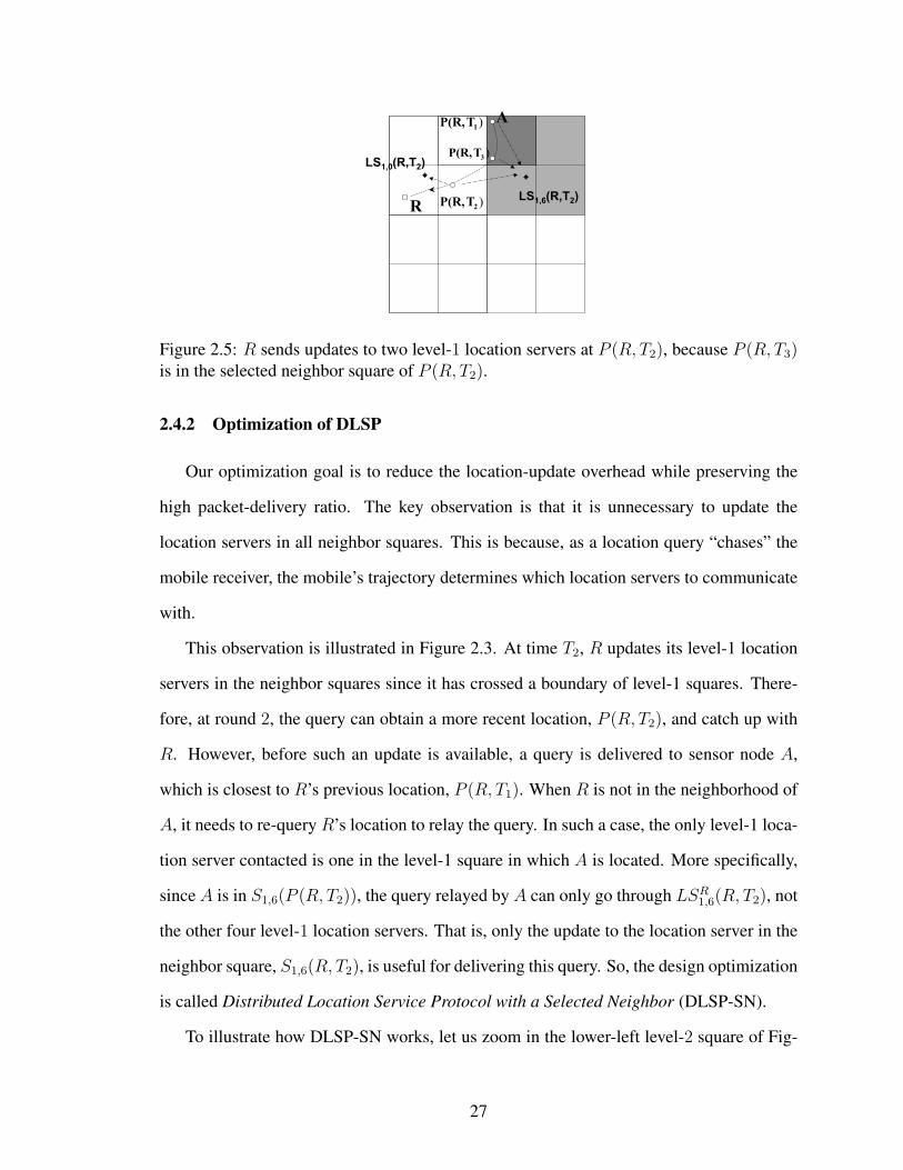
Figure 2.5: R sends updates to two level-1 location servers at P (R, T2), because P (R, T3)is in the selected neighbor square of P (R, T2).
2.4.2 Optimization of DLSP
Our optimization goal is to reduce the location-update overhead while preserving the
high packet-delivery ratio. The key observation is that it is unnecessary to update the
location servers in all neighbor squares. This is because, as a location query “chases” the
mobile receiver, the mobile’s trajectory determines which location servers to communicate
with.
This observation is illustrated in Figure 2.3. At time T2, R updates its level-1 location
servers in the neighbor squares since it has crossed a boundary of level-1 squares. There-
fore, at round 2, the query can obtain a more recent location, P (R, T2), and catch up with
R. However, before such an update is available, a query is delivered to sensor node A,
which is closest to R’s previous location, P (R, T1). When R is not in the neighborhood of
A, it needs to re-query R’s location to relay the query. In such a case, the only level-1 loca-
tion server contacted is one in the level-1 square in which A is located. More specifically,
since A is in S1,6(P (R, T2)), the query relayed by A can only go through LSR1,6(R, T2), not
the other four level-1 location servers. That is, only the update to the location server in the
neighbor square, S1,6(R, T2), is useful for delivering this query. So, the design optimization
is called Distributed Location Service Protocol with a Selected Neighbor (DLSP-SN).
To illustrate how DLSP-SN works, let us zoom in the lower-left level-2 square of Fig-
27
ure 2.3 in Figure 2.5. Suppose R needs to send location updates to level-1 location servers
at P (R, T1), P (R, T3), and P (R, T2) consecutively. At P (R, T3), it checks if its previ-
ous location P (R, T1) was in the level-1 square, S1,0(P (R, T1)). If so, it only updates
LSR1,0(R, T1) (i.e., LSR1,6(R, T2). At P (R, T2), R finds that its previous location P (R, T3)
is in the neighbor square, S1,6(P (R, T2)), so it sends updates to both LSR1,0(R, T2) and
LSR1,6(R, T2). Note that the locations of two consecutive level-k updates must be in the
same level-k square or two neighbor level-k squares, because the movement threshold for
level-k updates, 2k−m`, is strictly less than the edge length of level-k square, 2k`.
The differences between DLSP and DLSP-SN are summarized as follows. First, sup-
pose the highest level is h. Then, DLSP updates LSR0,j1(R, T ) (j1 = 0, 1, . . . , 8), and
LSRk,j2(R, T ) (k = 1, 2, . . . , h − 1 and j2 = 0, 1, . . . , 8). DLSP-SN updates LSRk,0(R, T )
(k = 0, 1, 2, . . . , h), as well as the location server in the selected neighbor square. Sec-
ond, suppose ki and ki+1 are the levels of location servers through which a location query
obtains the destination mobile’s location at i and i + 1, respectively. In this case, DLSP
requires ki > ki+1, but DLSP-SN does not have this restriction. To avoid endless chasing,
DLSP-SN requires that, at each round, the query get more recent location information than
the previous round.
DLSP-SN is less restrictive in the sense of obtaining location information, because it
selects many fewer location servers than DLSP. As a result, DLSP-SN incurs more rounds
and longer query paths.
2.5 Adaptation of Location Service
DLSP-SN reduces its update overhead, but may extend the query path length, increasing
the data-delivery cost. This increase of data-delivery cost may become significant in case
of continuous data streams commonly seen in sensor network applications. To achieve
overall energy-efficiency with DLSP-SN, we propose an adaptive location-update scheme
in which a mobile adaptively sends its location updates based on the varying distribution
28

)T P(R, 1
R
1S 2
S
ALS0(R,T)
Figure 2.6: Location queries (or data packets) from S1 and S2 travel less hops during round1 with adaptive location updates.
and rate of the data sources. We then analyze the parameter configuration for the adaptation
to ensure a high query-delivery ratio and present a greedy algorithm to improve overall
energy-efficiency. Finally, we summarize the comparison among the hierarchical location
service protocols, DLSP, DLSP-SN, DLSP-ASN, and GLS.
2.5.1 Adaptive Location Updates
In a hybrid wireless network of stationary sensors and mobile actors, a mobile may
receive data from multiple data sources located in the areas of interest. The overhead of
querying the mobile’s location to forward data from these sources may be expensive if
they need to contact high-level location servers. Typically, the data sources in an area of
interest are often spatially close to one another. Thus, the cost of location-query can be
significantly reduced if the mobile’s location can be retrieved from the common low-level
location server. Therefore, to reduce the overhead of location-queries, a mobile selects and
updates a few location servers near the data sources in DLSP-ASN.
Figure 2.6 provides an illustrative example. Suppose sensor nodes, S1 and S2, reside
in the same level-0 square S0,0(S1)(= S0,0(S2)), and continuously report data to a mobile
R. Instead of sending location updates to S1 and S2 individually, R picks an adaptive
location server, ALSR0 (S1), in Sk,0(S1), and periodically sends updates to it as well as to
the other location servers. When S1 or S2 sends R data, a location query is processed
exactly the same as in Section 2.2 except for the first round. R’s location can be obtained
29
from ALSR0 (S1), instead of from the level-2 location server, LSR2,j(R, T1), as shown in
Figure 2.2. Thus, the data-delivery cost is reduced at the expense of extra adaptive location
updates.
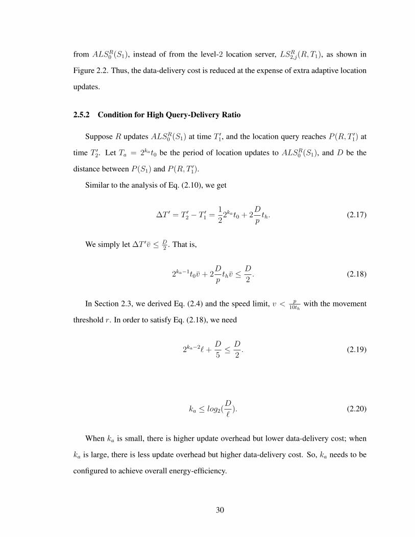
2.5.2 Condition for High Query-Delivery Ratio
Suppose R updates ALSR0 (S1) at time T ′1, and the location query reaches P (R, T ′1) at
time T ′2. Let Ta = 2kat0 be the period of location updates to ALSR0 (S1), and D be the
distance between P (S1) and P (R, T ′1).
Similar to the analysis of Eq. (2.10), we get
∆T ′ = T ′2 − T ′1 =1
22kat0 + 2
D
pth. (2.17)
We simply let ∆T ′v ≤ D2
. That is,
2ka−1t0v + 2D
pthv ≤
D
2. (2.18)
In Section 2.3, we derived Eq. (2.4) and the speed limit, v < p10th
with the movement
threshold r. In order to satisfy Eq. (2.18), we need
2ka−2`+D
5≤ D
2. (2.19)
ka ≤ log2(D
`). (2.20)
When ka is small, there is higher update overhead but lower data-delivery cost; when
ka is large, there is less update overhead but higher data-delivery cost. So, ka needs to be
configured to achieve overall energy-efficiency.
30
Prot
ocol
sD
LSP
DL
SP-S
ND
LSP
-ASN
GL
S
ID-t
o-L
Sm
appi
ngH
ash
the
mob
ileno
deID
into
alo
catio
nw
ithin
asq
uare
,an
dth
eno
decl
oses
tto
the
loca
tion
beco
mes
alo
catio
nse
rver
Sam
eas
DL
SPSa
me
asD
LSP
Sele
ctth
eno
dew
hose
IDis
clos
estt
oth
em
obile
node
IDw
ithin
asq
uare
LS
inne
ighb
orsq
uare
sO
neL
Sin
each
ofth
eei
ght
neig
hbor
squa
res
At
mos
ton
elo
catio
nse
rver
from
ane
ighb
orsq
uare
Sam
eas
DL
SP-S
NO
neL
Sfr
omea
chof
the
thre
ene
ighb
orsq
uare
s
Cro
ss-b
ound
ary
upda
tes
Loc
atio
nup
date
sca
non
lybe
trig
gere
dby
timeo
uts
orex
ceed
ing
the
mov
emen
tth
resh
old
Sam
eas
DL
SP,
but
the
se-
lect
edne
ighb
orde
pend
son
whe
ther
orno
tabo
unda
ryof
cert
ain
leve
lis
cros
sed
Sam
eas
DL
SP-S
NN
eed
toup
date
the
thre
ene
ighb
orlo
catio
nse
rver
sa
from
leve
l-0
tole
vel-k
ifth
ebo
unda
ryof
ale
vel-k
squa
reis
cros
sed
Dat
aso
urce
adap
tiven
ess
No
No
Yes
Am
obile
may
send
ad-
ditio
nal
loca
tion
upda
tes
toth
elo
catio
nse
rver
sne
arth
eda
taso
urce
sac
cord
ing
toa
gree
dyal
gori
thm
No.
Am
obile
node
may
send
itslo
catio
nto
the
data
sour
ces
ata
fixed
rate
Gri
ddin
gef
fect
No
Yes
Not
afte
rthe
addi
tiona
lloc
a-tio
nup
date
sar
ese
ntou
tY
es
Mul
ti-ro
unds
Yes
,with
rest
rict
ions
(1-3
)bY
es,w
ithre
stri
ctio
ns(1
-2)b
Sam
eas
DL
SP-S
NN
o
Tabl
e2.
2:C
ompa
riso
nof
hier
arch
ical
loca
tion
serv
ices
a InG
LS,
one
squa
reco
nsid
ers
itsth
ree
adja
cent
squa
res
belo
ngin
gto
the
sam
epa
rent
squa
reas
itsne
ighb
ors;
inD
LSP
prot
ocol
s,al
lthe
eigh
tadj
acen
tsqu
ares
are
cons
ider
edne
ighb
ors.
b Res
tric
tions
:(1
)T
hequ
ery
need
sto
obta
ina
new
erlo
catio
nof
the
mob
ileat
each
roun
d;(2
)th
equ
ery
does
notp
roce
edif
the
loca
tion
isob
tain
edfr
oma
leve
l-0
loca
tion
serv
erin
the
prev
ious
roun
d;(3
)the
leve
loft
helo
catio
nse
rver
sge
tslo
wer
asth
ero
und
prog
ress
es.
31

2.5.3 Analysis of Overall Energy-Efficiency
Let E denote the energy-efficiency without adaptive location updates, and Ea denote
the efficiency with adaptive location updates. The mobile maintains a moving window
to compute the average data rate, Rdata, the average hop count, Chops, and the average
distance, Dsrc, from the two sources.
∆E = Rdata ·(Chops −
Dsrc
p
)− Dsrc
p
1
2kat0(2.21)
A mobile periodically searches for ka in [0, log2
(D`
)] such that ∆E is maximized or
Ea is minimized.
In general, the rate and distribution of data sources cannot be described in a simple
form. It is, therefore, very difficult to compute the optimal solution that combines data
sources and sets ka for each combination. The mobile can use some simple heuristics to
find good solutions. For example, only the data sources in the same level-0 are combined
at their level-0 location server. We can then use the above analysis to set ka for each level-0
location server.
2.5.4 Comparison of Hierarchical Location Services
Different hierarchical location services are compared and summarized in Table 2.2.
2.6 Evaluation
We have performed extensive simulation to comparatively evaluate the performance of
location-service protocols. For this purpose, we have implemented the DLSP protocols
(DLSP, DLSP-SN, and DLSP-ASN) and GHLS in ns-2 [2] (version 2.27), and also have
ported GLS to the same version of ns-2 we used for other protocols.
The following metrics are evaluated for the location service protocols: (1) Query Deliv-
ery Ratio—the percentage of location queries successfully delivered to the mobile receiver;
32

(2) Update Overhead—the number of update packets transmitted with each hop counted as
one packet transmission; (3) Query Path Length—the number of hops each successfully-
delivered query takes.
2.6.1 The Simulation Setup
The transmission range for radio communication is set to 100m based on the charac-
teristics of MicaZ [1] devices. We assume the radio link is symmetric, and only collision
may cause message loss. Typically, the raw radio of sensor nodes (e.g., Mica2, MicaZ) is
lossy and asymmetric, but the underlying MAC or routing protocols provide reliable trans-
mission via scheduling and retransmission. We use both 802.11 MAC and S-MAC in our
simulation. We also use the two-ray ground propagation model.
Sensors are uniformly deployed over a square area, with density of 6.25 nodes per 100×
100m2. This high node density is chosen because in low node-density networks, geographic
routing (e.g., GPSR) suffers from relatively high packet losses, which may distract the
readers from our main focus on the performance of location services. Given this high node
density, the average per-hop progress is approximately 0.7r or 70m. Our tests are run on
networks of 400× 400, 800× 800, 1200× 1200, and 1600× 1600m2, which include 100,
400, 900, and 1600 sensor nodes, respectively. Since interactions among mobiles are not
considered, only one mobile is simulated in our evaluation, and its movement follows the
modified random way-point mobility model [78] in our base-case scenarios. The mobile’s
speed ranges from 4 to 40m/s, and its pause time is set to 0. We also simulate DLSP with
random walk and Guass-Markov mobility models [9] to confirm that the proposed protocol
functions regardless of the mobiles’ movement pattern. We also simulated DLSP using the
scenarios with 100×100 and 200×200 m2 void areas to show its resilience to node failures.
Finally, we evaluated DLSP with low-density networks.
We use GPSR [33] as a routing protocol throughout the evaluation of DLSP. The beacon
period is set to 10s for stationary sensor nodes and 1s for the mobile. When a sensor node
33
receives a beacon from the mobile, it replies with a beacon after a random delay ranging
from 0 to 1s. The movement threshold for triggering location updates in DLSP, DLSP-SN,
GHLS, and GLS is set to 100m (i.e., m = 1). The timeout for triggering location updates
for the location service protocols except for GLS (i.e., τ ) is 8s. GLS does not have any
timeout. Instead of using its instantaneous speed, the mobile uses its average speed over a
moving window. Suppose R sends two consecutive updates to its level-k location servers
at time T and T ′. The average speed v = dist(P (R,T ),P (R,T ′))T ′−T , although R’s trajectory may
follow an arbitrary curve. To determine the timeout for the location information sent to
a level-k location server, the mobile uses the average speed to predict the update interval
tk = 2kt0 with Eq. (2.3).
The edge length of the smallest square in the DLSP protocols (i.e., `) is 200m. In
GLS, the smallest square size is set to 100m, because all nodes in the same smallest square
should be within two hops. The network size we tested, 1200 × 1200m2, does not result
in a perfect grid structure. In such a case, if an intended level-k square is not within the
network boundary, it is substituted by a neighbor level-k square inside the boundary. For
example, the level-2 square may be outside the boundary when the mobile is located at
(900m,900m). Then, the level-2 square {(0,0), (800m,800m)} becomes its replacement.
Ten sensor-node deployments are generated for each network size. With each deploy-
ment, we generate a movement scenario for each speed. All test results are the averages
of 10 runs on all the deployments. Since the mobile’s ID is the same in all tests, a seed is
randomly generated in each run so that a sensor node can hash the mobile’s ID into a differ-
ent value for DLSP and GHLS. As for the workload, a sensor node is randomly chosen to
send a location query to the mobile once every 2s during a period of 200s, i.e., 100 queries
are sent. All tests for the same network size use the same workload. In GLS, every node
should publish its location information to its location servers for the correct functioning of
GLS. For fair comparison, we modify GLS such that the sensor nodes publish their location
only during the initial warm-up period of 120s. These location updates during the warm-up
34

Figure 2.7: The query-delivery ratio ofDLSP is higher than 96% for all networksizes if the mobile’s speed ≤ 15m/s. Thespeed limit from our analysis is 14m/s.
Figure 2.8: The query-delivery ratio ofDLSP-SN is close to that of DLSP belowthe speed limit, and noticeably better in caseof high speeds.
period are not counted in the update overhead.
For all protocols, the workload starts at 120s and the simulation ends at 300s. The
surplus of 80s allows the last few queries to be delivered.
2.6.2 Simulation Results Using 802.11 MAC
Using the 802.11 MAC in ns-2, the transmission time plus the backoff delays ranges
from 0.001 to 0.02s. Without a low-power MAC at hand, we add a fixed link-layer delay
of 0.5s (or 0.25s). Thus, the actual per-hop latency ranges from 0.5 to 0.52s (or 0.25 to
0.27s), which resembles the per-hop latency in low-power MACs [43, 75]. Because the
average per-hop progress of a packet is about 70m, the average packet-transmission speed
is calculated to be 140m/s. Based on our analysis, the speed limit with the movement
threshold of 100m is 14m/s.
2.6.2.1 Query-Delivery Ratio
Figure 2.7 shows that DLSP scales well if the mobile’s speed ≤ 15m/s. In the network
of 1600 nodes, the delivery ratios of both DLSP and DLSP-SN drop below 90% beyond
35
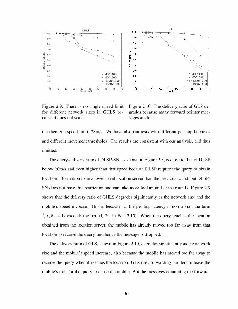
0 5 10 15 20 25 30 35 40 450
10
20
30
40
50
60
70
80
90
100
speed (m/s)
Del
iver
y R
atio
(%
)
GHLS
400x400800x8001200x12001600x1600
Figure 2.9: There is no single speed limitfor different network sizes in GHLS be-cause it does not scale.
Figure 2.10: The delivery ratio of GLS de-grades because many forward pointer mes-sages are lost.
the theoretic speed limit, 28m/s. We have also run tests with different per-hop latencies
and different movement thresholds. The results are consistent with our analysis, and thus
omitted.
The query-delivery ratio of DLSP-SN, as shown in Figure 2.8, is close to that of DLSP
below 20m/s and even higher than that speed because DLSP requires the query to obtain
location information from a lower-level location server than the previous round, but DLSP-
SN does not have this restriction and can take more lookup-and-chase rounds. Figure 2.9
shows that the delivery ratio of GHLS degrades significantly as the network size and the
mobile’s speed increase. This is because, as the per-hop latency is non-trivial, the term
2Lpthv easily exceeds the bound, 2r, in Eq. (2.15). When the query reaches the location
obtained from the location server, the mobile has already moved too far away from that
location to receive the query, and hence the message is dropped.
The delivery ratio of GLS, shown in Figure 2.10, degrades significantly as the network
size and the mobile’s speed increase, also because the mobile has moved too far away to
receive the query when it reaches the location. GLS uses forwarding pointers to leave the
mobile’s trail for the query to chase the mobile. But the messages containing the forward-
36
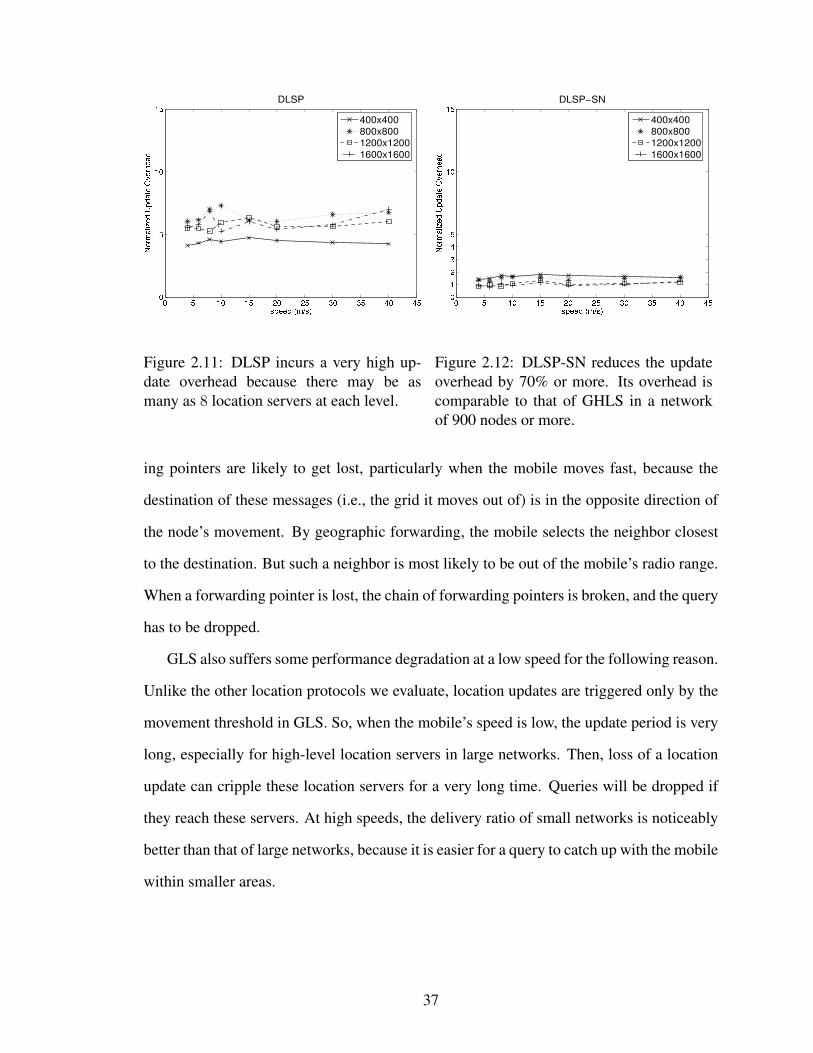
Figure 2.11: DLSP incurs a very high up-date overhead because there may be asmany as 8 location servers at each level.
Figure 2.12: DLSP-SN reduces the updateoverhead by 70% or more. Its overhead iscomparable to that of GHLS in a networkof 900 nodes or more.
ing pointers are likely to get lost, particularly when the mobile moves fast, because the
destination of these messages (i.e., the grid it moves out of) is in the opposite direction of
the node’s movement. By geographic forwarding, the mobile selects the neighbor closest
to the destination. But such a neighbor is most likely to be out of the mobile’s radio range.
When a forwarding pointer is lost, the chain of forwarding pointers is broken, and the query
has to be dropped.
GLS also suffers some performance degradation at a low speed for the following reason.
Unlike the other location protocols we evaluate, location updates are triggered only by the
movement threshold in GLS. So, when the mobile’s speed is low, the update period is very
long, especially for high-level location servers in large networks. Then, loss of a location
update can cripple these location servers for a very long time. Queries will be dropped if
they reach these servers. At high speeds, the delivery ratio of small networks is noticeably
better than that of large networks, because it is easier for a query to catch up with the mobile
within smaller areas.
37

Figure 2.13: GLS incurs a very high updateoverhead because each level has 3 locationservers, and boundary-crossing incurs addi-tional overhead.
Figure 2.14: DLSP-SN has longer querypaths due to gridding effect.
2.6.2.2 Location-Update Overhead
Because GHLS is shown in [12] to incur the least update overhead, we normalize the up-
date overheads of DLSP, DLSP-SN, and GHLS with respect to that of GHLS, as illustrated
in Figures 2.11–2.13. We obtained the results from the same tests for the query-delivery ra-
tio. All the normalized overheads are relatively insensitive to the mobile’s speed, since the
tests of all protocols use the same movement threshold for triggering location updates. As
the mobile’s speed increases, the update overhead increases accordingly for all protocols.
Compared to DLSP, DLSP-SN reduces the update overhead by at least 70%, as shown
in Figures 2.11 and 2.12. More importantly, the normalized overhead of DLSP-SN de-
creases as the network size increases because the normalized overhead of DLSP isO( log(N)N
)
(overhead of DLSP-SN is O(log(N)) and that of GHLS is O(N)). For this reason, GLS
exhibits a similar trend in Figure 2.13. However, the trend is not clear for DLSP, which can
be explained as follows. Because of the network boundary, the number of location servers
at any level increases as the network size grows. For example, the average number of level-
0 (level-1) location servers increases from 4 to 6.25 (from 0 to 3) as N changes from 100 to
38
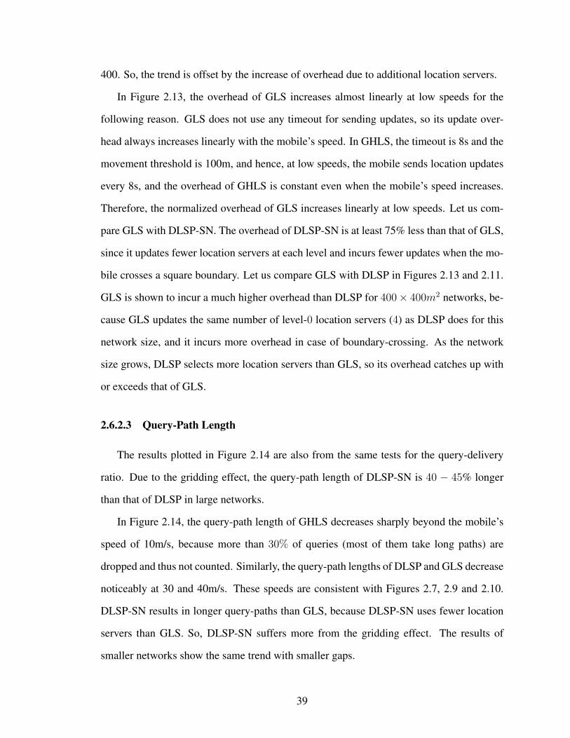
400. So, the trend is offset by the increase of overhead due to additional location servers.
In Figure 2.13, the overhead of GLS increases almost linearly at low speeds for the
following reason. GLS does not use any timeout for sending updates, so its update over-
head always increases linearly with the mobile’s speed. In GHLS, the timeout is 8s and the
movement threshold is 100m, and hence, at low speeds, the mobile sends location updates
every 8s, and the overhead of GHLS is constant even when the mobile’s speed increases.
Therefore, the normalized overhead of GLS increases linearly at low speeds. Let us com-
pare GLS with DLSP-SN. The overhead of DLSP-SN is at least 75% less than that of GLS,
since it updates fewer location servers at each level and incurs fewer updates when the mo-
bile crosses a square boundary. Let us compare GLS with DLSP in Figures 2.13 and 2.11.
GLS is shown to incur a much higher overhead than DLSP for 400× 400m2 networks, be-
cause GLS updates the same number of level-0 location servers (4) as DLSP does for this
network size, and it incurs more overhead in case of boundary-crossing. As the network
size grows, DLSP selects more location servers than GLS, so its overhead catches up with
or exceeds that of GLS.
2.6.2.3 Query-Path Length
The results plotted in Figure 2.14 are also from the same tests for the query-delivery
ratio. Due to the gridding effect, the query-path length of DLSP-SN is 40 − 45% longer
than that of DLSP in large networks.
In Figure 2.14, the query-path length of GHLS decreases sharply beyond the mobile’s
speed of 10m/s, because more than 30% of queries (most of them take long paths) are
dropped and thus not counted. Similarly, the query-path lengths of DLSP and GLS decrease
noticeably at 30 and 40m/s. These speeds are consistent with Figures 2.7, 2.9 and 2.10.
DLSP-SN results in longer query-paths than GLS, because DLSP-SN uses fewer location
servers than GLS. So, DLSP-SN suffers more from the gridding effect. The results of
smaller networks show the same trend with smaller gaps.
39

0 5 10 15 20 25 30 35 40 450
10
20
30
40
50
60
70
80
90
100Delivery Ratio w/Adaptation
speed (m/s)
Del
iver
y R
atio
DLSP−ASNDLSP−SNGHLS
Figure 2.15: The delivery ratios of DLSPand GHLS match the results in previous fig-ures.
0 5 10 15 20 25 30 35 40 450
0.5
1
1.5
2
2.5Normalized Total Energy Cost w/Adaptation
speed (m/s)
Nor
mal
ized
Ene
rgy
Cos
t
DLSP−ASNDLSP−SN
Figure 2.16: The energy cost of DLSP-ASNis even less than GHLS when the speedis below 15m/s, when both provide highpacket-delivery ratios.
2.6.2.4 Adaptation
To evaluate how DLSP-ASN improves overall energy-efficiency over DLSP-SN, we
use the same deployments and movements as in previous tests, but change the workload
such that only two sensor nodes in the same level-0 square send data to the mobile at the
same constant rate.
Figures 2.15 and 2.16 show the results from a network of 1600 nodes and the data rate
of 0.5 message per 1 second for each node.
Figure 2.15 shows that, with adaptive location updates, DLSP-ASN has a slightly higher
delivery ratio than DLSP-SN, because, in the first round, each query travels fewer hops
in DLSP-ASN than in DLSP-SN. So it takes less time for a query to reach the mobile’s
known location, and thus, the mobile moved away less from the location. Starting at the
second round, the query has a higher chance to be delivered successfully. Figure 2.16 shows
the total energy cost normalized by the total cost of GHLS. Here we use the number of
transmissions as the energy cost since we use the same transmission power for all packets.
The adaptive mechanism can improve the overall energy-efficiency by as much as 40%.
40

For the range of 4 to 15m/s, the total energy cost of DLSP-ASN is comparable to, or even
lower than, that of GHLS. This is because most queries are delivered in one round. During
the first round, a query obtains the mobile’s location information within a small square in
DLSP-ASN, but in GHLS, it has to travel more hops to a randomly-picked location server
within the largest square. As the speed increases, the improvement diminishes because
DLSP-ASN also needs to take more rounds to deliver the queries. In the tests of smaller
networks and lower data rates, DLSP-ASN shows less improvement on overall efficiency
as expected.
2.6.3 Simulation Results Using S-MAC
In order to validate our analysis of DLSP on a MAC with real low-power duty cycling,
we simulated DLSP using S-MAC [76]. S-MAC is inspired by PAMAS [61] and uses RTS-
CTS to reduce channel contention. S-MAC periodically sleeps, wakes up to receive and
transmit packets if any, and then returns to sleep. Each active period is a constant period,
and thus, the length of the sleep period determines the length of each frame (i.e., the active
period plus the sleep period). To match the per-hop latency with our 802.11 MAC-based
simulation, we set the sleep period such that the length of the S-MAC duty cycle is 0.5s.
Other parameters of S-MAC such as slot time are kept as default, resulting in 20.8% duty
cycle. This duty cycle is rather high, but we keep the default parameters of S-MAC while
setting the per-hop delay as 0.5s for a fair comparison.
Moreover, because S-MAC is designed for static sensor networks, we need to slightly
modify it to deal with mobility — if a sensor node receives a beacon from a mobile, it stays
awake for a short period (in our simulation, this period is 2.5s). With this modification,
the neighbor sensors of the mobile are given enough wakeup time to send their replies
and avoid severe collision, which could occur without the modification. The mobile node
does not observe S-MAC sleep-scheduling, so it can communicate with sensor nodes with
different sleep schedules. This may be justified because the mobile is usually much less
41

Network Average Standard Movementsize per-hop latency deviation threshold
400m × 400m 0.251s 0.271 27.9m/s800m × 800m 0.373s 0.281 18.8m/s
1200m × 1200m 0.410s 0.280 17.1m/s1600m × 1600m 0.439s 0.313 16.0m/s
Table 2.3: Average per-hop latency of DLSP using S-MAC. The average per-hop latencyand its standard deviation vary with the network size. The movement thresholds can thusbe derived from our analysis using Eq. 2.13 for different network sizes.
power-constrained than sensors.
If a packet is lost, the sender tries to send it again (up to 3 times) in the next active
period. Therefore, the actual per-hop latency varies with sleep scheduling and packet re-
transmission. The results presented next are from the test runs using the same deployments
and movements as in the previous simulation.
Unlike the DLSP simulation with 802.11 MAC with fixed delay of 0.5s, DLSP with S-
MAC can have a delay shorter than its frame length (which is set to 0.5s) for the following
reasons. First, the sensors surrounding the mobile node stay awake longer than other sensor
nodes, so the latency between these sensors and the mobile is much less than that between
two sensors under low-power duty cycling, which is approximately 0.5s. Second, at the
origin of each packet, the per-hop latency is, on average, half of a duty cycle. As the
network size increases, location updates and queries take more sensor-to-sensor hops, so
the average per-hop latency increases. The mean and standard deviation of the per-hop
latency and the speed limit derived from Eq. 2.13 are shown in Table 2.3.
Figures 2.17–2.19 plot the query-delivery ratio of DLSP, DLSP-SN, and GHLS, re-
spectively, using S-MAC. With S-MAC, the performance of DLSP protocols (DLSP and
DLSP-SN) also validates our analysis — DLSP protocols scale well if the mobile’s speed is
under the limit as shown in Table 2.3, and degrade as the mobile’s speed grows beyond the
movement threshold. Compared to Figures 2.7, 2.17 shows that the performance of DLSP
with S-MAC is slightly better than that of DLSP with 802.11-MAC, while the performance
42
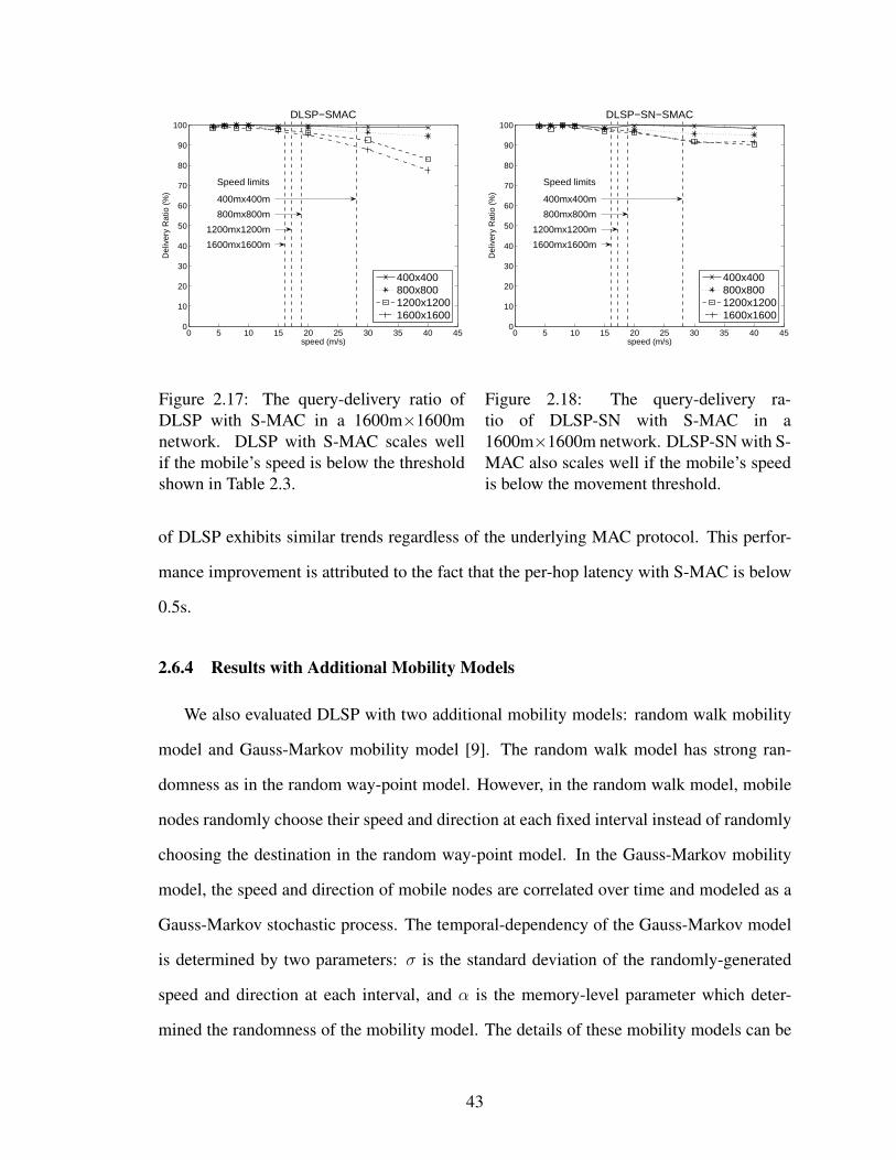
0 5 10 15 20 25 30 35 40 450
10
20
30
40
50
60
70
80
90
100
speed (m/s)
Del
iver
y R
atio
(%
)
DLSP−SMAC
400mx400m
800mx800m
1200mx1200m
1600mx1600m
Speed limits
400x400800x8001200x12001600x1600
Figure 2.17: The query-delivery ratio ofDLSP with S-MAC in a 1600m×1600mnetwork. DLSP with S-MAC scales wellif the mobile’s speed is below the thresholdshown in Table 2.3.
0 5 10 15 20 25 30 35 40 450
10
20
30
40
50
60
70
80
90
100
speed (m/s)
Del
iver
y R
atio
(%
)
DLSP−SN−SMAC
400mx400m
800mx800m
1200mx1200m
1600mx1600m
Speed limits
400x400800x8001200x12001600x1600
Figure 2.18: The query-delivery ra-tio of DLSP-SN with S-MAC in a1600m×1600m network. DLSP-SN with S-MAC also scales well if the mobile’s speedis below the movement threshold.
of DLSP exhibits similar trends regardless of the underlying MAC protocol. This perfor-
mance improvement is attributed to the fact that the per-hop latency with S-MAC is below
0.5s.
2.6.4 Results with Additional Mobility Models
We also evaluated DLSP with two additional mobility models: random walk mobility
model and Gauss-Markov mobility model [9]. The random walk model has strong ran-
domness as in the random way-point model. However, in the random walk model, mobile
nodes randomly choose their speed and direction at each fixed interval instead of randomly
choosing the destination in the random way-point model. In the Gauss-Markov mobility
model, the speed and direction of mobile nodes are correlated over time and modeled as a
Gauss-Markov stochastic process. The temporal-dependency of the Gauss-Markov model
is determined by two parameters: σ is the standard deviation of the randomly-generated
speed and direction at each interval, and α is the memory-level parameter which deter-
mined the randomness of the mobility model. The details of these mobility models can be
43
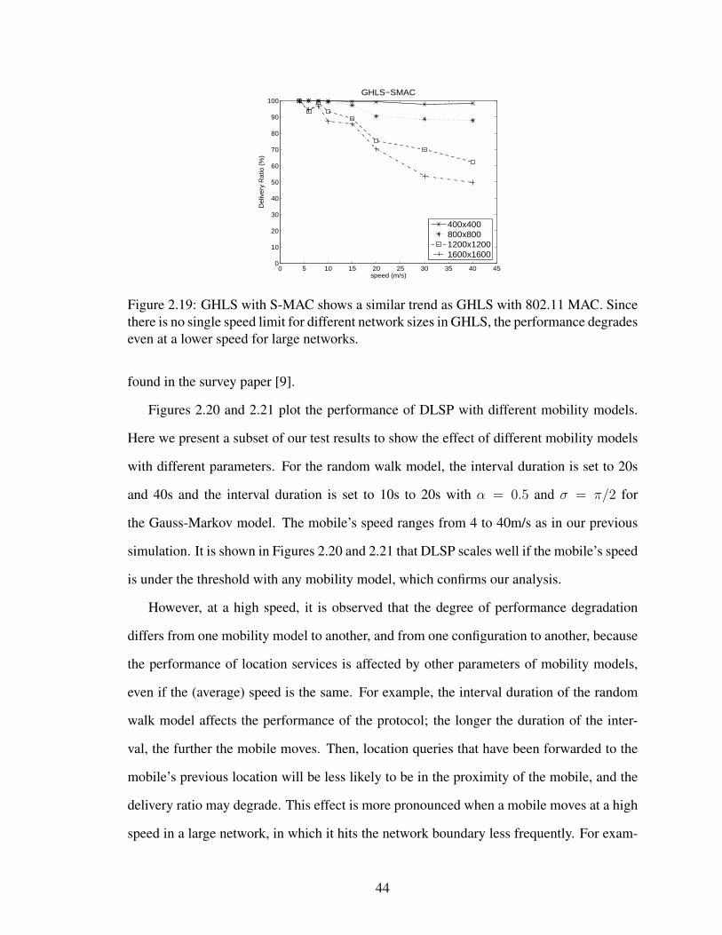
0 5 10 15 20 25 30 35 40 450
10
20
30
40
50
60
70
80
90
100
speed (m/s)
Del
iver
y R
atio
(%
)
GHLS−SMAC
400x400800x8001200x12001600x1600
Figure 2.19: GHLS with S-MAC shows a similar trend as GHLS with 802.11 MAC. Sincethere is no single speed limit for different network sizes in GHLS, the performance degradeseven at a lower speed for large networks.
found in the survey paper [9].
Figures 2.20 and 2.21 plot the performance of DLSP with different mobility models.
Here we present a subset of our test results to show the effect of different mobility models
with different parameters. For the random walk model, the interval duration is set to 20s
and 40s and the interval duration is set to 10s to 20s with α = 0.5 and σ = π/2 for
the Gauss-Markov model. The mobile’s speed ranges from 4 to 40m/s as in our previous
simulation. It is shown in Figures 2.20 and 2.21 that DLSP scales well if the mobile’s speed
is under the threshold with any mobility model, which confirms our analysis.
However, at a high speed, it is observed that the degree of performance degradation
differs from one mobility model to another, and from one configuration to another, because
the performance of location services is affected by other parameters of mobility models,
even if the (average) speed is the same. For example, the interval duration of the random
walk model affects the performance of the protocol; the longer the duration of the inter-
val, the further the mobile moves. Then, location queries that have been forwarded to the
mobile’s previous location will be less likely to be in the proximity of the mobile, and the
delivery ratio may degrade. This effect is more pronounced when a mobile moves at a high
speed in a large network, in which it hits the network boundary less frequently. For exam-
44

0 5 10 15 20 25 30 35 40 450
10
20
30
40
50
60
70
80
90
100
speed (m/s)
Del
iver
y R
atio
(%
)
DLSP w/mobility models in 800mx800m network
RWPRW20RW40GM10GM20
Figure 2.20: The random way-point model(RWP), the random walk model (RWP)with the duration of 20s (RW20) and 40s(RW40), and the Gauss-Markov modelwith the duration of 10s (GM10) and 20s(GM20) are simulated with DLSP in an800m×800m network.
0 5 10 15 20 25 30 35 40 450
10
20
30
40
50
60
70
80
90
100
speed (m/s)
Del
iver
y R
atio
(%
)
DLSP w/mobility models in 1600mx1600m network
RWPRW20RW40GM10GM20
Figure 2.21: The random way-point model(RWP), the random walk model (RWP)with the duration of 20s (RW20) and 40s(RW40), and the Gauss-Markov modelwith the duration of 10s (GM10) and 20s(GM20) are simulated with DLSP in an1600m×1600m network.
ple, in Figure 2.21, it is shown that the random walk mobility model with a 20s duration
(RW20) outperforms the same model with a 40s duration (RW40) at 40m/s. So does the
Gauss-Markov mobility.
There are previous efforts to develop the common metrics that can interpret the param-
eters of different mobility models [58,81], but not a single good metric has been developed
yet, and most of them focused on routing protocols, not on location services. Development
of a universal measure of mobility models for location services is beyond the scope of this
work.
2.6.5 Results on Robustness Against Node Failures
We evaluated the robustness of DLSP when some sensor nodes fail. By modifying the
scenarios used before, we introduced a void area that contains no functional node. We
picked the void area such that the mobile node passes through the area at 30 seconds in
simulation time, i.e., the mobile goes through the void area at least once. The size of the
45
0 5 10 15 20 25 30 35 40 450
0.2
0.4
0.6
0.8
1
speed (m/s)
Nor
mal
ized
del
iver
y ra
tio
Normalized delivery ratio with a 100m−by−100m void area
400x400800x8001200x12001600x1600
(a) The normalized delivery ratio when a void area of100m×100m is introduced.
0 5 10 15 20 25 30 35 40 450
0.2
0.4
0.6
0.8
1
speed (m/s)
Nor
mal
ized
del
iver
y ra
tio
Normalized delivery ratio of with a 200m−by−200m void area
400x400800x8001200x12001600x1600
(b) The normalized delivery ratio when a void area of200m×200m is introduced.
Figure 2.22: The delivery ratios with void areas are normalized to that of the scenariowithout any void area. These plots show that the delivery ratio of DLSP degrades slightlywhen a void area is introduced. The delivery ratio degrades more as the void area getsrelatively larger, i.e., the network becomes smaller or the void area becomes bigger orboth.
void area is chosen to be of 100× 100 or 200× 200 m2.
Figure 2.22 shows the delivery ratio with a void area, which is normalized to that
with no void area shown in Figure 2.17. When a 100×100m2 void area is introduced,
the delivery ratio drops slightly (up to 2.39%) as shown in Figure 2.22(a). Figure 2.22(b)
shows the normalized delivery ratio when a 200× 200m2 void area is introduced. With the
200 × 200m2 void area, the average degradation of delivery ratio is higher, ranging from
4.43% to 9.16%. The delivery ratio decreases as network size increases (i.e., the relative
size of the void area decreases). These figures show that DLSP performs well even with a
void area.
The performance degradation is due to the following two reasons: (1) some location
update/query messages are more likely to be lost while the mobile is in a void area, and
(2) some update/query messages may have to detour around the void area, causing some
message loss (decrementing TTL down to zero) or extending their end-to-end delay and
hence making it harder for them to catch up with the mobile.
If the size of a void area is relatively large, according to its random movement, the
46
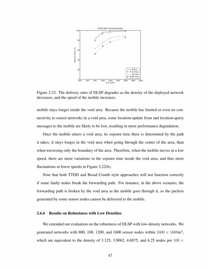
400 600 800 1000 1200 1400 1600 1800 2000# of nodes
0
20
40
60
80
100
Deliv
ery
Rati
o (
%)
DLSP with varying density
8 m/s15 m/s30 m/s40 m/s
Figure 2.23: The delivery ratio of DLSP degrades as the density of the deployed networkdecreases, and the speed of the mobile increases.
mobile stays longer inside the void area. Because the mobile has limited or even no con-
nectivity to sensor networks in a void area, some location-update from and location-query
messages to the mobile are likely to be lost, resulting in more performance degradation.
Once the mobile enters a void area, its sojourn time there is determined by the path
it takes; it stays longer in the void area when going through the center of the area, than
when traversing only the boundary of the area. Therefore, when the mobile moves at a low
speed, there are more variations in the sojourn time inside the void area, and thus more
fluctuations at lower speeds in Figure 2.22(b).
Note that both TTDD and Bread Crumb style approaches will not function correctly
if some faulty nodes break the forwarding path. For instance, in the above scenario, the
forwarding path is broken by the void area as the mobile goes through it, so the packets
generated by some sensor nodes cannot be delivered to the mobile.
2.6.6 Results on Robustness with Low Densities
We extended our evaluation on the robustness of DLSP with low-density networks. We
generated networks with 800, 100, 1200, and 1600 sensor nodes within 1600 × 1600m2,
which are equivalent to the density of 3.125, 3.9062, 4.6875, and 6.25 nodes per 100 ×
47

Number of nodes in800 1000 1200 1600
1600m×1600m areaAverage per-hop
62.71 71.11 75.94 80.88progress (m)
Table 2.4: Average per-hop progress with varying numbers of nodes in 1600m×1600mnetworks.
100m2. The networks with less than 800 nodes are often disconnected, and thus excluded
in our evaluation.
As shown in 2.23, the delivery ratio degrades as the node density is decreased or as the
mobile’s speed is increased. This is because, as the network gets sparser, the average per-
hop progress becomes smaller and the messages travel longer paths. It therefore becomes
harder for messages to catch up with the mobile destination. This effect can be severer
when a mobile moves with higher speeds.
This result also confirms our analysis; DLSP achieves a high packet-delivery ratio when
the average per-hop progress is above 70m/s (the speed used in our analysis) and a mobile’s
speed is below its speed limit, 15m/s. The average per-hop progress with the different node
density is shown in Table 2.4. In networks with 1000 or more nodes, the average per-hop
progress is above 70m/s. In such networks, the delivery ratios of DLSP for the mobile’s
speed of of 8m/s and 15 m/s are 98.40% and 96.70%, respectively.
2.7 Conclusion
In this chapter, we presented a distributed location service protocol (DLSP) which con-
siders the non-trivial per-hop latency caused by low-power duty cycling in sensor networks.
Through a rigorous analysis of DLSP, we derive the condition for achieving a high packet-
delivery ratio, and show how to configure the protocol parameters to ensure the scalability
of DLSP. DLSP is shown to be scalable if the mobile’s speed is below a certain fraction of
the packet-transmission speed, which depends on a movement threshold. The theoretical
mobile’s speed limit is a one-fifth of the packet-transmission speed.
48

We evaluate DLSP with extensive simulation using two MAC protocols and three mo-
bility models. The evaluation results confirm our analysis. We also proposed an opti-
mization technique, DLSP-SN, that can reduce the location-update overhead by 70% or
more, while its query-delivery ratio is even better than DLSP when the mobile’s speed
is high. In order to make a tradeoff between update and data-delivery costs, we pre-
sented a greedy adaptation mechanism, DLSP-ASN, which can significantly improve over-
all energy-efficiency. DLSP is also shown to be robust in the scenarios with void areas or
node failures.
49
CHAPTER III
DISTRIBUTED HOLE DETECTION
3.1 Introduction
Recently, WSNs are being deployed in various applications such as environmental mon-
itoring, emergency rescue, object tracking, traffic monitoring and control, healthcare appli-
cations, and building-integrity monitoring.
A hole in a WSN can be defined as an area which is not covered by a communication
or sensing range of any sensor node in the network. A formal definition of a hole is given
in Section 3.4. Holes in a WSN can be formed for various reasons. First, holes form due
to the characteristics of the deployment area. If a sensor network is deployed in a field or
urban setting, obstacles such as lakes or buildings will create holes. Second, holes may be
formed due to events. For example, in a sensor network for detecting a fire in a forest, holes
may represent the area where fire has occurred. Third, holes may be generated by faulty
and depleted nodes. Finally, holes may be formed when an active attacker destroys or jams
an area.
The detection of such holes in a WSN is important because 1) the holes themselves can
represent valuable information such as characteristics of deployment areas or the event of
interest, and 2) the holes can significantly affect the performance of many protocols that
use location information. For example, in geographic forward routing, detouring around a
hole, such as a perimeter mode of a greedy perimeter stateless routing (GPSR) [33], can be
50
a very expensive process. Also in data centric storage (DCS) [24, 27, 42, 56], the election
of storage nodes may not be possible if the hashed location for a certain event is within
certain holes. In such a case, the performance of DCS can be poor or the protocol may not
even function.
The current approaches to hole detection can be categorized into range-free and range-
based approaches. The former [21, 41] exploits only connectivity information for hole
detection, while the latter [18] exploits geographic location information from sensor nodes.
Although range-free approaches do not require a localization service, they are inefficient for
detecting newly-generated or enlarged holes because they require expensive network-wide
flooding procedures to detect any change in network topology. On the other hand, range-
based approaches [18] require a localization service. The localization service is not an extra
overhead for various sensor network applications, since they too require the geographic
location of sensor nodes. However, an unrealistic unit-disk model is adopted in [18], which
does not discuss location estimation errors or link asymmetry.
We propose a distributed hole detection algorithm that utilizes location information.
The proposed algorithm is designed for applications that require knowing the geographic
location of sensor nodes and prompt detection of newly-generated or enlarged holes, for
such applications as the fire detection. The real-time availability of the information of areas
affected by fire is important. The proposed algorithm will depend only on local information
of node locations for detecting holes in a WSN. Also, the proposed algorithm will be able
to tolerate the location errors and asymmetry of the communication ranges among sensor
nodes.
The contributions in this chapter are threefold as follows. First, we propose a distributed
algorithm, TRAVERSE, to detect the hole boundaries. It exploits the information of the
realistic radio and localization models. Second, we suggest geographic forward routing
with hole avoidance (GFRHA) to detour packets around holes. GFRHA uses the hole
information detected by TRAVERSE to route packets before they encounter the holes, to
51

reduce path lengths and energy consumption. Finally, we evaluate TRAVERSE and GFRHA
with qualitative and quantitative metrics. We first evaluate TRAVERSE for topologies with
holes of various shapes, and then for varying network density, or with varying parameters
of the radio model. We also evaluate GFRHA against a well-known geographic forwarding
algorithm, GPSR, to show its performance gain in the presence of holes.
The rest of this chapter is structured as follows. In Section 3.2, we summarize the
related work. After introducing the assumptions in Section 3.3, we present the details of our
distributed hole detection algorithm in Section 3.4. In Section 3.5, we discuss GFRHA as
an application of the proposed protocol. Section 3.6 shows the qualitative and quantitative
evaluations of our approach. Finally, we conclude this chapter in Section 3.7.
3.2 Related Work
In the range-free hole-detection algorithms, the location of sensor nodes is not used.
Instead, the connectivity information is used to detect holes. In the range-based algorithm,
the location of sensor nodes is used to determine the boundary of each hole on the network.
Range-free approaches [21,41] flood the network from a small number of beacon nodes.
Holes are identified using hop-count discrepancies from those beacon nodes. A few addi-
tional flooding procedures are necessary to tighten the boundary of the detected holes. This
approach is claimed to be more efficient, since it does not require a localization service and
the number of flooding procedures is limited [41]. However, detecting newly generated or
enlarged holes with this approach may not be efficient because it requires a few network-
wide flooding procedures to identify new boundaries of holes upon changes in network
topology.
Range-based approaches [18] require the location information of each node, since their
detection mechanism depends on the location information of sensor nodes. However, the
localization service is not an extra overhead for various sensor network applications, since
they too require the geographic location of sensor nodes. Thus, location information is
52
already available without any overhead for those applications. For example, the aforemen-
tioned fire-detection application will require the geographic location of the sensor nodes
where a fire occurred. However, in [18], an unrealistic unit-disk model is adopted, which
does not discuss location estimation errors or link asymmetry.
A hole detection problem also appeared in graph theory [29, 50]. However, the defini-
tion of a hole in graph theory is not same as that of our problem. In graph theory, a hole is
defined as a chordless cycle with five or more vertices, where a chordless cycle is defined
as a sequence of k distinct vertices, v0, v1, · · · , vk−1 in which there is an edge from vi to
v(i+1) mod k (for all i = 0, · · · , k − 1), and no other edge between any two of these vertices.
When nodes and links between them are represented as vertices and edges, respectively, the
holes in the sensor networks are identified as holes in graph theory. However, a chordless
hole may not correspond to any hole in a WSN. Even though a chordless hole corresponds
to a hole in the WSN, the chordless hole may not be a tight bound of a hole in a WSN.
Thus, we modified the definition of hole in graph theory to fit our problem. Our formal
definition of hole will be given in Section 3.4.
Motion planning [37] is one of the fields in robotics that has several similarities with
our problem, where a problem of navigating robots avoiding obstacles is studied. Typi-
cally, motion planning takes two phases: mapping and planning. A map of a given area
is obtained in the mapping phase, and actual movement pattern is evaluated in the plan-
ning phase. A map of the given area is often obtained by using multiple sensor-readings,
or by exploration of automated robots. Then, an optimal path to a destination location is
evaluated using the obtained map.
Our hole-detection is similar to the mapping phase, and GFRHA is similar to the plan-
ning phase; we first find holes (obstacles) in the given area, and then, route messages
instead of navigating robots avoiding the detected holes. However, there are several dif-
ferences between motion planning and our problem. In motion planning, mapping and
planning is done by resourceful robots. In the mapping phase, they directly interact with
53
multiple sensors, or explore the area by themselves, and in the planning phase, they eval-
uate the optimal (or near-optimal) path to the destination using a global map obtained in
the mapping phase. In our problem, since sensor nodes are resource-limited and have only
limited local views instead of a globe view of the deployment area, they should collaborate
to detect holes, and use local views to route messages around holes.
Nonetheless, there are algorithms, called bug algorithms, that use only limited local
views as in our algorithms proposed in this chapter. Among bug algorithms, VisBug is
similar to GFR; in VisBug, robots are navigated in the direction of a destination until they
encounter an obstacles, and then around the obstacles using only local information. Also,
TagentBug is similar to our algorithm, GFRHA; in TangentBug, robots are navigated in the
tangential direction of an obstacle if it lies between the current position and the destination.
The difference between TangentBug and our algorithms are twofold. First, in TRAVERSE,
sensor nodes distributively detect holes, while robots can directly detect the boundary of
obstacles by using a visibility sensor in TagentBug. Second, the detected hole information
should be disseminated to nearby sensor nodes, while this procedure is not required since
robots have the obstacle information obtained with their own visibility sensors.
3.3 System Assumptions
3.3.1 Radio Model
In WSNs, wireless channels show irregularities on radio performance as in other wire-
less channels [49,82]. The irregularities are very common in wireless communication, and
they are caused by many factors, such as different path losses, depending on propagation di-
rections, radio transmission power, and interferences with other nodes. These irregularities
result in non-uniform transmission ranges, asymmetric communication links, etc.
The unit-disk model is a simple disk model, but cannot capture the dynamics of wireless
channels. Under the unit-disk model, the radio transmission range is a perfect circle; all the
54
nodes in the network have a uniform transmission range, and there is a link between two
nodes if they are located within the transmission range. Thus, this model cannot represent
the realistic performance of a WSN.
Here, we adopt the log-normal shadowing radio propagation model [49] to capture the
irregularities of wireless channels, in which the received signal strength is modeled with
the log-normal distribution. More specifically, the reception power P at distance r from
the transmitting node with the transmission power p0 is defined by
P = p0
(r0
r
)α10X/10,
where r0 is the reference distance for the antenna far-field, α the path loss exponent, and
X ∼ N(0, σ2), where σ is the shadowing deviation. This model is identical to the unit-disk
model when σ = 0. The threshold distance is defined as one from which the received
signal strength starts to drop below the threshold power, under which the receiver cannot
decode signals when σ = 0. As in [49], we also define the connection function, φ(r), as
the probability that a receiver at distance r from the sender can decode the signal. The
connection function for the log-normal distribution is given by
φ(r) = Pr
[X ≥ 10α ln(r/rt)
ln(10)
]=
1
2− 1
2erf(
10α ln(r/rt)√2 ln(10)σ
).
Since our proposed algorithm requires two-way communications, we assume that there
exists a link between two nodes with the probability of φ(r)2 when the distance between
them is r.
55

3.3.2 Localization Service Model
Localization services in sensor networks have gained popularity because they provide
location information essential to numerous sensor network applications. Localization ser-
vices estimate the location of each sensor node using the relative distance or direction
among sensor nodes and optional anchor nodes with exact location information. Relative
distance or directions among neighboring nodes are obtained using difference-in-time-of-
arrival, received signal strength, or connectivity. Typically, localization service iterates the
estimation process several times to achieve a high level of precision in location estimation
as required by the applications. Also, there may exist anchor (or beacon) nodes which have
the exact location information loaded manually or obtained by using GPS-like devices.
These anchor nodes provide their exact location information to sensor nodes in their vicin-
ity, and this location information acts as the seed of the location information for normal
sensor nodes. Using anchor nodes reduces the errors of the location estimation and/or the
number of iterations to achieve the same level of precision in location estimation.
Here, we assume that the location estimation error can be modeled as a normal distri-
bution. In other words, the majority of location estimations for the sensor nodes are close
to the exact locations of the sensor nodes. Also, we assume that the standard deviation of
the normal distribution is smaller than, or comparable to, the average communication range
of sensor nodes. If the location estimation errors are too large, not only our hole detection
algorithm, but also other routing protocols or applications running atop the localization
service, will not function correctly. Thus, this assumption is reasonable for most WSN
applications.
56
3.4 Distributed Hole Detection
3.4.1 Overview
We first define a hole in WSNs using graph theory. Nodes and links between nodes are
represented as vertices and edges, respectively. On the graph, a hole is defined as a cycle
with certain properties.
Based on this definition of a hole, we present an algorithm called TRAVERSE to detect
the boundary of each hole. The algorithm is designed to be distributed so that it can be
invoked efficiently and immediately upon each topology change. Also, it is designed to
function with errors in location estimation, or the realistic radio model, such as the log-
normal radio propagation model. jj The process of detecting holes is composed of three
steps. First, we identify nodes that may be on the boundary of holes, called boundary
candidate nodes. The condition for the candidate nodes will be discussed in the following
subsection. Second, we identify the boundary of each hole by starting from the candidate
node. TRAVERSE is designed to identify the boundary of each hole. Third, we detect
enlarged or newly-generated holes by invoking TRAVERSE upon topology change.
The rest of this section is organized as follows. The definition of a hole in WSN is
given in Section 3.4.2. We describe the identification of candidate nodes in Section 3.4.3,
followed by a description of handling special cases in Section 3.4.4. The main algorithm,
TRAVERSE, is introduced in Section 3.4.5. Finally, we describe the detection of a new hole
or the change of a hole in Section 3.4.6.
3.4.2 Definition of a Hole
Here, we formally define a hole before discussing hole detection. We first define some
terminologies, and use them to define a hole.
We introduce a graph representation of a sensor network for concise description of our
problem. A deployed sensor network can be represented as a graph G = (V,E), where
57

sensor nodes and links between sensor nodes are represented as vertices and edges, respec-
tively. Since geographic location of vertices in a graph G is important for hole definition,
we also consider G as a subset of R2, where the vertices in G have the same geographic
location, or 2-D coordinates, as they have in a deployed sensor network. The deployed
senor network can be considered as the graph G’s geometric realization of R2. We define
a hole with both geographic- and graph-representation of the deployed network.
We now define terminologies needed for hole definition.
Definition 1. Let C be a sequence of vertices of length k, v0, v1, · · · , vk−1. We define C as
a non-intersecting cycle if there is an edge from vi to vi+1 mod k (for all i = 0, · · · , k − 1)
and no edge in the cycle intersects with another edge.
Definition 2. A non-intersecting cycle C divides the plane into two regions. We define the
region on the right side of the cycle as the inside of the cycle if we traverse the cycle in the
same order of the given sequence of the cycle. The other region is defined as the outside of
the cycle.
Now we define a chordal path as follows.
Definition 3. For a non-intersecting cycle C, consider a path P with the following condi-
tions. First, P is a sequence of vertices, w0, w1, · · · , w`−1. Second, there exist non-adjacent
vertices vi and vj such that w0 = vi and w`−1 = vj . Third, for all p (0 < p < `− 1), there
does not exist any q (0 ≤ q ≤ k − 1) such that wp = vq. If there exists a path P satisfying
all of the above conditions, we define such a path as a chordal path of the cycle C.
We can now define a hole in a WSN with the above terms as follows.
Definition 4. We define a non-intersecting cycle C as a hole if it has no chordal path inside
the cycle. Also, we define the edges of the cycle as the boundary of the hole.
For a given hole, we also define the following terminologies.
58

Figure 3.1: This figure shows examples of holes.
Definition 5. A hole is defined as an inner hole if the order of the vertices in the cycle is
clockwise. The boundary of an inner hole is defined as an inner boundary. Similarly, we
define a hole as an outer hole if the order of the vertices in the cycle is counterclockwise,
and its boundary as an outer boundary. Inner boundaries define the boundaries of holes
inside the deployment area, and outer boundaries define the boundaries of the network
deployment area.
Definition 6. We define node vi and node vk as the incoming node and the outgoing node
for node vj , respectively, when there is a partial path such as · · · , vi, vj, vk, · · · in a hole
boundary.
We now clarify the definition of a hole with an example shown in Figure 3.1. For
example, a cycle v1, v2, v3, v4, v5 is a hole since there is no chordal path inside the cycle.
Also, this cycle is an inner hole since the order of vertices is clockwise. On the other hand,
a cycle v1, v5, v4, v3, v2 is not a hole since there are chordal paths inside the cycle; a path
v1, v6, v7, v2 is one such chordal path.
Now let us consider a cycle v6, v10, v9, v8, v7. Since there is no chordal path inside the
cycle, this cycle is a hole. Note that vertices v1, v2, · · · , v5 are outside of this cycle. This
cycle is an outer hole, and it defines the boundary of the deployment area.
Depending on the application or the network service which uses the boundary infor-
mation, very small holes are insignificant. For example, the performance of geographic
59

routing protocols are not affected by very small holes. Thus, it may be useful to have
thresholds for a hole such that only holes relevant for the application are identified. We
define a hole of a length k or more as a k-length hole. Similarly, we can define A-area hole
as a hole of size equal to or greater than A, where the area of a given hole is defined as the
area of the inside (outside) for an inner (outer) hole.
3.4.3 Identification of Candidate Nodes
As a preparation process of TRAVERSE, we identify the boundary candidate nodes.
Boundary candidate nodes are the nodes which may lie on the boundary of holes. Then,
TRAVERSE will be initiated from each candidate node.
From the definition of a k-length hole, it is obvious that the boundary of a k-length hole
is an `-side polygon, where ` ≥ k. In such a polygon, we have the following property.
Lemma III.1. The sum of angles inside an `-gon is given as π·(`−2). Thus, there is at least
an inner angle that is equal to, or greater than, π·(`−2)/`. Since π·(`−2)/` ≥ π·(k−2)/k
if ` ≥ k. Therefore, there is at least an inner angle that is equal to, or greater than,
π · (k − 2)/k among nodes on the boundary of a hole of length of `(≥ k).
We define a candidate node based on Lemma III.2.
Definition 7. Let v0 be a node with p neighbors, v1, v2, · · · , vp. Without loss of generality,
we assume that v1, v2, · · · , vp are in the counterclockwise order from v0. We also let
vp+1 = v1. We define the node v0 as a candidate node if there exists i, 1 ≤ i ≤ p such
that ∠viv0vi+1 ≥ π · (k − 2)/k, where k is the threshold of a hole. Here, we also define
vi and vi+1 as an incoming node and an outgoing node of the candidate node. Note that a
candidate node may have more than one pair of incoming-outgoing nodes.
From the definition of candidate node, we have the following property.
Lemma III.2. For each hole in a WSN, there exists at least one candidate node, v, in the
hole boundary. Also, v and v’s incoming and outgoing nodes belong to the hole boundary.
60

v1
v2
v3
v4
v5
v6v7
v0
Figure 3.2: This figure shows examples of candidate nodes.
Proof. From Lemma III.1, at least one of inner angles of a hole is equal to, or greater than,
π · (k − 2)/k. Since every node that has such angles at it is identified, there exists at least
one candidate node for each hole boundary.
Thus, candidate nodes can be identified using information about immediate neighbors.
Note that when a node on a hole boundary is identified as a candidate node, its incoming
node and outgoing node are also in the boundary of the hole. Also, note that a node may
identify itself even though it is not in a hole boundary. This may happen when the length
of the minimum cycle including the identified node and its incoming and outgoing nodes
is smaller than the threshold k. Also, it may happen to a node that belongs to BRIDGE or
CAPE, which will be defined in Section 3.4.4.
Figure 3.2 shows the example of a candidate node. We will use a node v0 as an example
node. It first sort its neighbor nodes with the counterclockwise angular order. Here, the
result will be v1, v2, v3, v4, and v5. When k = 5, ∠v1v0v2 and ∠v4v0v5 are greater than
π · (k − 2)/k = 0.6π = 108◦. Thus, v0 is identified as a candidate node, and v1-v2 and
v4-v5 are identified as incoming-outgoing pairs of the candidate node v0. We may need to
invoke TRAVERSE more than once from the candidate node v0 since it has more than one
61

Figure 3.3: The special cases handled by the TRAVERSE algorithm.
pairs of incoming-outgoing nodes.
3.4.4 Handling Special Cases
After identifying the candidate nodes, we handle some special cases before invoking
the hole traverse algorithm.
First, we identify nodes which have only one neighbor. From each such nodes, we start
traversing following the neighbor of the node until we find a node which has more than
two neighbors. We call this path CAPE. Figure 3.3(a) shows examples of CAPES with
the length of two. CAPES may exist on the boundaries of holes or network area, and the
number of CAPES may increase as the density of the network decreases. We exclude the
nodes in CAPES with the exception of the last one, which has more than two neighbors,
when identifying the boundaries of holes since these nodes will give the dead-ends.
Second, we remove the candidate node information if a node has only two neighbors.
This node belongs to either a CAPE or a BRIDGE. BRIDGE as shown in Figure 3.3(b) is
defined as a path between two boundaries of different holes if only one path exists between
the two boundaries. The detailed discussion of BRIDGE will follow in the following sub-
section. If this node belongs to a CAPE, this node will not be on the boundary of any hole,
as explained above. If this node belongs to a BRIDGE, this node will be identified as a
node on the boundary by starting TRAVERSE from another node. In both cases, it is not
62
necessary to start TRAVERSE from nodes which have only two neighbors. Thus, we do not
start TRAVERSE from these nodes.
Finally, we remove the hole of length three. For every candidate node, we check if the
incoming node of the candidate node is a neighbor of the outgoing node of the candidate
node. In other words, the hole formed by the candidate node is a simple triangle. Thus, we
eliminate this case since the hole caused by such a candidate node is trivial.
3.4.5 Identification of hole boundary
After identifying candidate nodes, we identify a boundary for each hole by traversing
from candidate nodes. Basically, we follow the boundary of holes using the right hand
rule as in [18]. However, we need to enhance the traversing method to accommodate the
realistic radio model.
We present the TRAVERSE algorithm to identify the boundary of holes. In essence,
TRAVERSE forwards a message starting from a candidate node using the right-hand rule
to follow the boundary of a hole in a clockwise direction. When starting TRAVERSE,
we apply the right-hand rule from the incoming node of the candidate node, which will
result in an outgoing node. Note that a candidate node can have more than one pair of
incoming–outgoing nodes. In such a case, we may need to invoke TRAVERSE for each
pair of incoming–outgoing nodes. For example, in Figure 3.2, v0 will initiate TRAVERSE
with v1 − v2 and v4 − v5 as incoming–outgoing node pairs. After initiating TRAVERSE,
we repeat the use of the right-hand rule until we reach the starting node. If we reach the
starting node while traversing a hole, the path generated by TRAVERSE is identified as the
boundary of the hole, and TRAVERSE will terminate. In the example shown in Figure 3.2,
the boundary for the v1 − v2 pair will be found by the order of v0, v2, v6, v7, v1, and v0 by
using the right-hand rule. This algorithm is similar to BOUNDHOLE algorithm in [18], but
has different rules in handling special cases such as edge intersections and loops.
In TRAVERSE, we do not allow edge intersections. If the link between the current node
63
and the next node to follow dictated by the right-hand rule intersects any of the link in the
path of the current traverse, we do not follow the link. Instead we apply the right-hand rule
repeatedly until we find a link which does not intersect any of the links in the path of the
current traverse. It is possible that every outgoing link intersects with the current traverse
path. In this case, we abandon the last node in the path, and go back to the second last
node in the path. At the second last node, we find the next best node other than the last
node in the path, and follow the node. This process is called back tracking. The length
of cycles identified by TRAVERSE may be smaller than the threshold k. Information about
such small cycles is not required by applications, and thus, it is abandoned.
Now, we will show the property and the correctness of TRAVERSE.
Lemma III.3. When TRAVERSE is invoked at a candidate node on a hole, it finds the hole
containing the candidate node and its incoming–outgoing node pair.
Proof. A node that belongs to either BRIDGE or CAPE does not invoke TRAVERSE. Thus,
TRAVERSE is invoked only when it and its incoming and outgoing nodes belong to the
boundary of a hole. Note that a hole may be shorter than the threshold k, which should be
checked after identifying the hole.
TRAVERSE will first follow the outgoing node of the given candidate node by the right-
hand rule. Finding the next node using the right-hand rule is repeated until the starting
candidate node is reached. Since, in TRAVERSE, edge intersection is not allowed when
selecting the next node, it will follow the hole boundary without breaking it. Also, due to
the back tracking, TRAVERSE will continue to follow the hole boundary in case there is no
node to follow, which may happen when all the edges from a certain node are intersecting
the hole boundary.
Now, we will prove there is not any chordal path inside the cycle. Let us assume that
there exists a chordal path P, w1, w2, · · · , wp, inside a cycle C, v1, v2, · · · , vk, identified by
TRAVERSE. Letw1 be vi, which is one end of the chordal path P. For concise representation,
we also let v0 and vk+1 be vk and v1, respectively. Since the chordal path is inside the cycle
64
C from the assumption, i.e., the nodes in P are in the right side of the cycle, ∠vi−1w1w2 =
∠vi−1viw2 < ∠vi−1vivi+1. However, in such a case, the next node chosen by TRAVERSE at
the node vi should have been w1 instead of vi+1 by the right-hand rule. This contradiction
comes from the assumption that there exists a chordal path. Therefore, there does not exist
a chordal path in the cycle identified by TRAVERSE.
Now we can prove the correctness of TRAVERSE.
Theorem III.4. TRAVERSE finds every hole in the deployed network.
Proof. From Lemma III.2, it is proved that TRAVERSE will be initiated from at least one
node from every hole in the network. Then, as proved in Lemma III.3, TRAVERSE identifies
a cycle without chordal paths. Thus, the cycle identified by TRAVERSE is a hole if its length
is greater than the threshold k. Therefore, with the identification of candidate nodes and
TRAVERSE, every hole in the network is identified.
Also, we find the next node to traverse by looking at up to two-hop neighbors to find
tight bounds. Under the unit-disk model, it may suffice to consider only 1-hop neighbor as
in [18]. However, in a real scenario, a topology as shown in Figure 3.4 may exist in the net-
work due to the location estimation error or non-uniform radio transmission range. In such
a case, there may be a tighter bound than the hole boundary found by TREAVERSE using
only 1-hop neighbor. Note that the latter boundary is also a hole by definition. Thus, we
consider the location of up to two-hop neighbors, and the node as the next traversing node
which has a neighbor in the traversing direction. For example, in Figure 3.4(a), TRAVERSE
considers up to two-hop neighbors when selecting the next node to follow. When the cur-
rent path is · · ·− i− j, node n will be selected as the next node to follow since its neighbor
o is preferred to node l by the right-hand rule. However, a certain two-hop neighbor of the
current node which seems better by the right-hand rule may not be a preferable choice. In
Figure 3.4(b), when the current path is · · · − i − j − k, node i, a two-hop neighbor of k
is preferred to node l or node m by the right-hand rule. However, selection of this node is
65

j
k
l
no
i
m
p
j
k
l
no
i
m
p
(a) When the current path is · · · − i − j, node nwill be selected as the next node to follow since itsneighbor o is preferred to node l by the right-handrule.
k
l
m
j
n
i
k
l
m
j
n
i
(b) When the current path is · · · − i − j − k, thenode l is selected as the next node to follow insteadof node n because node i, a neighbor of node n,goes back to the node in the current path.
Figure 3.4: Examples of cases to consider two-hop neighbor lookups when TRAVERSE
selects the next node to follow.
not preferred since it goes back to the previous path. To avoid such a case, we check if the
two-hop neighbor is not on the left-side of the following path. For example, if k chooses
n as its next node to follow, node i is on the left-side of the segment k − n. Thus, node i
through node n is not a preferable choice to follow.
While traversing, we may form a loop in the path as shown in Figure 3.3(c). This
case often occurs when we traverse the network boundary. In this case, we remove the
loop from the current traverse path, and the loop is identified as a boundary of another
hole. After separating the identified loop into another boundary of a hole, we continue the
traversing from the node where the loop is found using, again, the right-hand rule.
A special case of the boundary may include the BRIDGE. BRIDGE is defined as a path
between the boundaries of different holes if only one path exists between them as shown in
Figure 3.3(b). A BRIDGE is identified by TRAVERSE when it detects a loop, and it cannot
find any other link to follow but the link in the traverse path. In this case, we trace back our
traverse path until we can find another link to follow. Then, we continues TRAVERSE from
that node, and the path in the BRIDGE is removed from the boundary.
66

3.4.6 Detection of Topology Changes
TRAVERSE will be invoked shortly after the initial deployment to identify the routing
holes introduced by the environment, such as terrain or non-uniform deployment. However,
while the sensor networks are operating, the topology of the sensor networks may change
because of faulty nodes, events in the network, or active attack. Thus, new holes may
be generated or the existing holes may be enlarged. These topology changes should be
recognized, and the boundary information should be updated as necessary.
In most sensor network protocols, each sensor nodes periodically broadcasts heart-
beat packets to ensure its availability to its immediate neighbors. When a node misses
consecutive heart-beat packets more than a predefined threshold from one of its neighbors,
it regards the neighbor node failed, and removes it from its neighbor list.
When a node detects a failure of its neighbor, TRAVERSE can be invoked in the follow-
ing cases to reflect the change in topology of the sensor networks. First, TRAVERSE will
be invoked if a node becomes a candidate node after missing one or more of its neighbors.
In this case, TRAVERSE will run normally as in the initial hole detection phase.
Second, TRAVERSE can be invoked if one of the nodes in a boundary of a hole detects
its outgoing node failed. In this case, we set an update flag to enforce the hole detection
since the nodes in the boundary already have the boundary information.
3.5 Geographic Forward Routing with Hole Avoidance
3.5.1 Overview
We now discuss utilizing the hole boundary information identified by TRAVERSE. As
an example application utilizing hole information, we modify the geographic forward rout-
ing (GFR) protocol such that packets are detoured around holes. As a baseline GFR proto-
col, we will use GPSR [33].
While a packet is forwarded near a hole by GPSR, it can be the case that the node which
67
holds the packet does not have any neighbor node closer to the destination location. In such
a case, GPSR needs to start an expensive hole detouring algorithm. For example, in such as
case, GPSR enters perimeter mode, and routes the packet to the nodes using the right-hand
rule in a planarized graph.
However, packets can be detoured before they encounter a hole instead of invoking
expensive perimeter-mode forwarding, if the boundary of holes identified by TRAVERSE
are known in advance. When a node forwards a packet, it can check if there exists a hole
between the node and the destination location. In such a case, it can detour the packet
around the hole instead of greedily forwarding the packet to the direction.
In the rest of this section, we discuss the utilization of hole information with more
details in Section 3.5.2, and then, show examples of the routing while detouring packets to
avoid holes in Section 3.6.2.
3.5.2 Detouring Messages Using Hole Information
We propose geographic forward routing with hole avoidance (GFRHA) as a potential
application of the hole information. GFRHA detours packets around holes before they
encounter a hole to avoid expensive perimeter-mode forwarding. To achieve this, we first
disseminate the identified hole information around the hole. Then, we detour the packet
utilizing the disseminated information as necessary.
When the boundary of a hole is identified by TRAVERSE, the summary of the boundary
information is disseminated to sensor nodes near the hole. After identifying a hole, we
approximate the identified hole as a circle which contains all the nodes on the boundary of
the hole. Then, we disseminate the summary of the hole, i.e., the coordinates of the center
and the radius of the approximated circle, to the nearby sensor nodes. More specifically, we
disseminated the summary information only to sensor nodes near the hole using controlled
flooding; when a sensor node receives such information, it rebroadcasts it only when it is
within a certain threshold distance from the center of the circle.
68
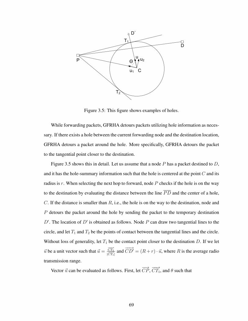
P
C
D
T2
T1
u
u1
u2
D’
Θ
Figure 3.5: This figure shows examples of holes.
While forwarding packets, GFRHA detours packets utilizing hole information as neces-
sary. If there exists a hole between the current forwarding node and the destination location,
GFRHA detours a packet around the hole. More specifically, GFRHA detours the packet
to the tangential point closer to the destination.
Figure 3.5 shows this in detail. Let us assume that a node P has a packet destined to D,
and it has the hole-summary information such that the hole is centered at the point C and its
radius is r. When selecting the next hop to forward, node P checks if the hole is on the way
to the destination by evaluating the distance between the line PD and the center of a hole,
C. If the distance is smaller than R, i.e., the hole is on the way to the destination, node and
P detours the packet around the hole by sending the packet to the temporary destination
D′. The location of D′ is obtained as follows. Node P can draw two tangential lines to the
circle, and let T1 and T2 be the points of contact between the tangential lines and the circle.
Without loss of generality, let T1 be the contact point closer to the destination D. If we let
~u be a unit vector such that ~u =−−→CT1
|−−→CT1|
and−−→CD′ = (R+ r) · ~u, where R is the average radio
transmission range.
Vector ~u can be evaluated as follows. First, let−→CP ,
−−→CT1, and θ such that
69

−→CP = ` · −→u1,
−→CT = r · −→u ,
θ = ∠PCT1,
where −→u1 and −→u are unit vectors.
Since PT1⊥CT1,−→CP ·
−−→CT1 = r2. From this, we get `−→u1 · r−→u = lr cos θ = r2. Thus,
−→u1 · −→u = cos θ = r/`.
Now let −→u2 a unit vector such that −→u1⊥−→u2, −→u = α−→u1 · β−→u2.
We can get α and β as follows.
−→CP ·
−−→CT1 = `−→u1 · r (α−→u1 + β−→u2)
= αr`−→u1 · −→u1 + βr`−→u1 · −→u2
= α`r
= r2
Thus,
α =r
`and β = ±
√`2 − r2
`.
Thus,
−→u =r
`−→u1 ±
√`2 − r2
`−→u2.
If the current node P or the destination location D is in the circle C, it just uses the
perimeter mode instead of detouring because there may not exist a path to D′.
70
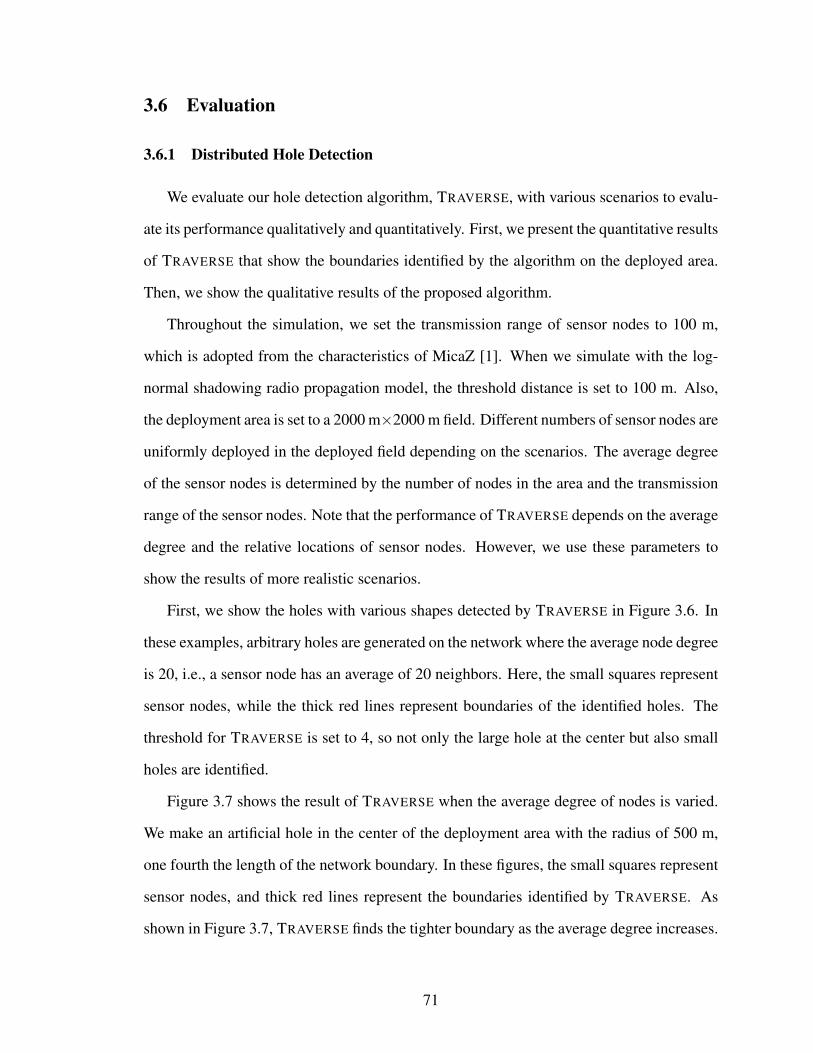
3.6 Evaluation
3.6.1 Distributed Hole Detection
We evaluate our hole detection algorithm, TRAVERSE, with various scenarios to evalu-
ate its performance qualitatively and quantitatively. First, we present the quantitative results
of TRAVERSE that show the boundaries identified by the algorithm on the deployed area.
Then, we show the qualitative results of the proposed algorithm.
Throughout the simulation, we set the transmission range of sensor nodes to 100 m,
which is adopted from the characteristics of MicaZ [1]. When we simulate with the log-
normal shadowing radio propagation model, the threshold distance is set to 100 m. Also,
the deployment area is set to a 2000 m×2000 m field. Different numbers of sensor nodes are
uniformly deployed in the deployed field depending on the scenarios. The average degree
of the sensor nodes is determined by the number of nodes in the area and the transmission
range of the sensor nodes. Note that the performance of TRAVERSE depends on the average
degree and the relative locations of sensor nodes. However, we use these parameters to
show the results of more realistic scenarios.
First, we show the holes with various shapes detected by TRAVERSE in Figure 3.6. In
these examples, arbitrary holes are generated on the network where the average node degree
is 20, i.e., a sensor node has an average of 20 neighbors. Here, the small squares represent
sensor nodes, while the thick red lines represent boundaries of the identified holes. The
threshold for TRAVERSE is set to 4, so not only the large hole at the center but also small
holes are identified.
Figure 3.7 shows the result of TRAVERSE when the average degree of nodes is varied.
We make an artificial hole in the center of the deployment area with the radius of 500 m,
one fourth the length of the network boundary. In these figures, the small squares represent
sensor nodes, and thick red lines represent the boundaries identified by TRAVERSE. As
shown in Figure 3.7, TRAVERSE finds the tighter boundary as the average degree increases.
71

0 500 1000 1500 2000
0
500
1000
1500
2000
(a) Circle0 500 1000 1500 2000
0
500
1000
1500
2000
(b) Square
0 500 1000 1500 2000
0
500
1000
1500
2000
(c) Rectangle0 500 1000 1500 2000
0
500
1000
1500
2000
(d) L-Shape
0 500 1000 1500 2000
0
500
1000
1500
2000
(e) U-Shape0 500 1000 1500 2000
0
500
1000
1500
2000
(f) Swirl
Figure 3.6: The result of TRAVERSE for the networks with holes of various shapes.
72

0 500 1000 1500 2000
0
500
1000
1500
2000
(a) Average degree is 80 500 1000 1500 2000
0
500
1000
1500
2000
(b) Average degree is 10
0 500 1000 1500 2000
0
500
1000
1500
2000
(c) Average degree is 150 500 1000 1500 2000
0
500
1000
1500
2000
(d) Average degree is 20
Figure 3.7: The result of TRAVERSE for the networks with varying average degree whenan artificial circular hole exists in the center of the deployment area. The small squaresrepresent the node in the deployed area, and the thick lines represent the boundaries iden-tified by the proposed algorithm. As the average degree increases, the boundaries found byTRAVERSE get tighter since more nodes exist close to the boundaries of the central holeand the network boundary.
73
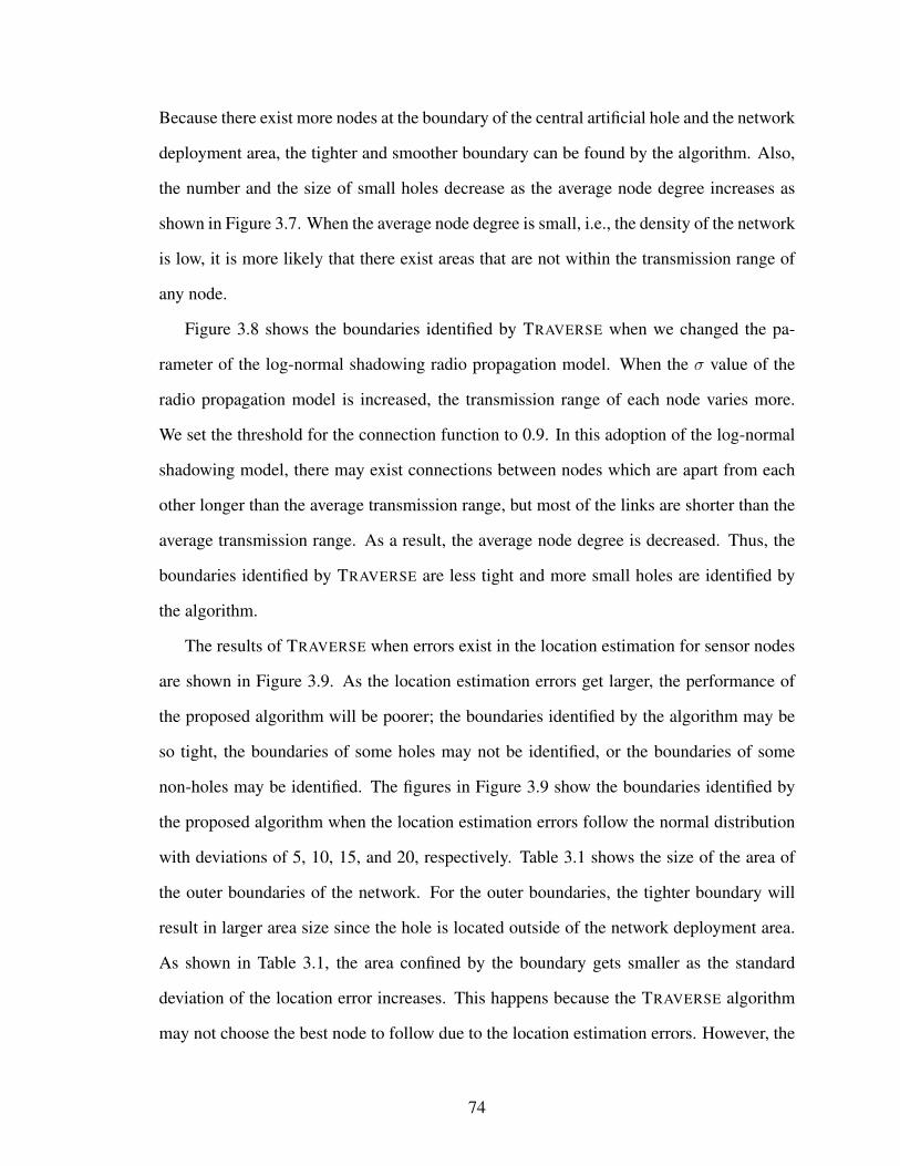
Because there exist more nodes at the boundary of the central artificial hole and the network
deployment area, the tighter and smoother boundary can be found by the algorithm. Also,
the number and the size of small holes decrease as the average node degree increases as
shown in Figure 3.7. When the average node degree is small, i.e., the density of the network
is low, it is more likely that there exist areas that are not within the transmission range of
any node.
Figure 3.8 shows the boundaries identified by TRAVERSE when we changed the pa-
rameter of the log-normal shadowing radio propagation model. When the σ value of the
radio propagation model is increased, the transmission range of each node varies more.
We set the threshold for the connection function to 0.9. In this adoption of the log-normal
shadowing model, there may exist connections between nodes which are apart from each
other longer than the average transmission range, but most of the links are shorter than the
average transmission range. As a result, the average node degree is decreased. Thus, the
boundaries identified by TRAVERSE are less tight and more small holes are identified by
the algorithm.
The results of TRAVERSE when errors exist in the location estimation for sensor nodes
are shown in Figure 3.9. As the location estimation errors get larger, the performance of
the proposed algorithm will be poorer; the boundaries identified by the algorithm may be
so tight, the boundaries of some holes may not be identified, or the boundaries of some
non-holes may be identified. The figures in Figure 3.9 show the boundaries identified by
the proposed algorithm when the location estimation errors follow the normal distribution
with deviations of 5, 10, 15, and 20, respectively. Table 3.1 shows the size of the area of
the outer boundaries of the network. For the outer boundaries, the tighter boundary will
result in larger area size since the hole is located outside of the network deployment area.
As shown in Table 3.1, the area confined by the boundary gets smaller as the standard
deviation of the location error increases. This happens because the TRAVERSE algorithm
may not choose the best node to follow due to the location estimation errors. However, the
74

0 500 1000 1500 2000
0
500
1000
1500
2000
(a) σ = 0.20 500 1000 1500 2000
0
500
1000
1500
2000
(b) σ = 0.5
0 500 1000 1500 2000
0
500
1000
1500
2000
(c) σ = 1.00 500 1000 1500 2000
0
500
1000
1500
2000
(d) σ = 2.0
Figure 3.8: The result of TRAVERSE for the networks with varying parameters for thelog-normal shadowing radio propagation model. As the value of σ is increased, the aver-age node degree is decreased, resulting in looser boundaries and more small holes in thedeployment area.
75
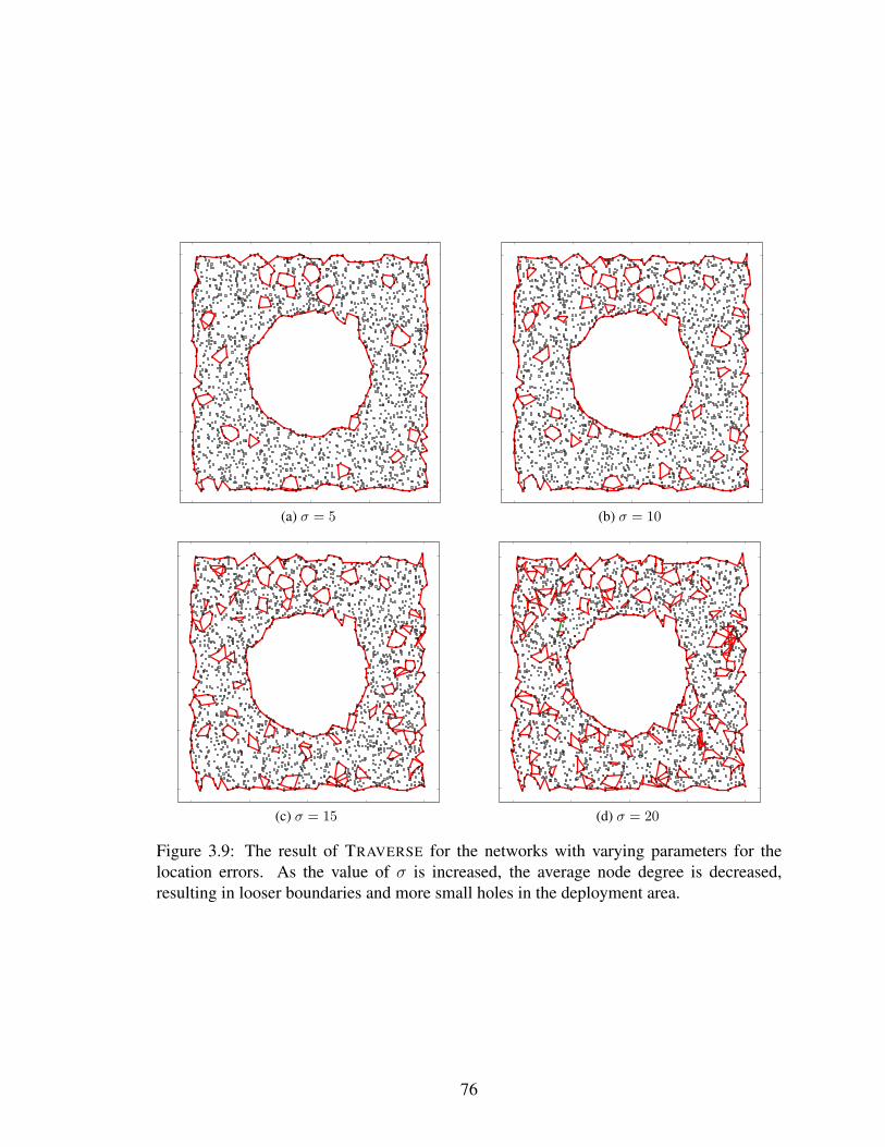
0 500 1000 1500 2000
0
500
1000
1500
2000
(a) σ = 50 500 1000 1500 2000
0
500
1000
1500
2000
(b) σ = 10
0 500 1000 1500 2000
0
500
1000
1500
2000
(c) σ = 150 500 1000 1500 2000
0
500
1000
1500
2000
(d) σ = 20
Figure 3.9: The result of TRAVERSE for the networks with varying parameters for thelocation errors. As the value of σ is increased, the average node degree is decreased,resulting in looser boundaries and more small holes in the deployment area.
76
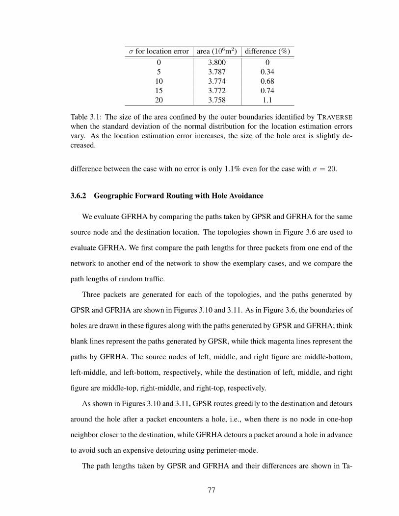
σ for location error area (106m2) difference (%)0 3.800 05 3.787 0.34
10 3.774 0.6815 3.772 0.7420 3.758 1.1
Table 3.1: The size of the area confined by the outer boundaries identified by TRAVERSE
when the standard deviation of the normal distribution for the location estimation errorsvary. As the location estimation error increases, the size of the hole area is slightly de-creased.
difference between the case with no error is only 1.1% even for the case with σ = 20.
3.6.2 Geographic Forward Routing with Hole Avoidance
We evaluate GFRHA by comparing the paths taken by GPSR and GFRHA for the same
source node and the destination location. The topologies shown in Figure 3.6 are used to
evaluate GFRHA. We first compare the path lengths for three packets from one end of the
network to another end of the network to show the exemplary cases, and we compare the
path lengths of random traffic.
Three packets are generated for each of the topologies, and the paths generated by
GPSR and GFRHA are shown in Figures 3.10 and 3.11. As in Figure 3.6, the boundaries of
holes are drawn in these figures along with the paths generated by GPSR and GFRHA; think
blank lines represent the paths generated by GPSR, while thick magenta lines represent the
paths by GFRHA. The source nodes of left, middle, and right figure are middle-bottom,
left-middle, and left-bottom, respectively, while the destination of left, middle, and right
figure are middle-top, right-middle, and right-top, respectively.
As shown in Figures 3.10 and 3.11, GPSR routes greedily to the destination and detours
around the hole after a packet encounters a hole, i.e., when there is no node in one-hop
neighbor closer to the destination, while GFRHA detours a packet around a hole in advance
to avoid such an expensive detouring using perimeter-mode.
The path lengths taken by GPSR and GFRHA and their differences are shown in Ta-
77

0 500 1000 1500 2000
0
500
1000
1500
2000
0 500 1000 1500 2000
0
500
1000
1500
2000
0 500 1000 1500 2000
0
500
1000
1500
2000
(a) Detouring circle
0 500 1000 1500 2000
0
500
1000
1500
2000
0 500 1000 1500 2000
0
500
1000
1500
2000
0 500 1000 1500 2000
0
500
1000
1500
2000
(b) Detouring square
0 500 1000 1500 2000
0
500
1000
1500
2000
0 500 1000 1500 2000
0
500
1000
1500
2000
0 500 1000 1500 2000
0
500
1000
1500
2000
(c) Detouring rectangle
Figure 3.10: An example of routing with hole-avoidance. In each figure, the boundariesof holes are drawn along with the summary of a hole by red line. Also the paths takenby GPSR and GFRHA are represented by a thin black line and a thick magenta line. Thesources of left, middle, and right figure are middle-bottom, left-middle, and left-bottom,respectively. The destination of left, middle, and right figure are middle-top, right-middle,and right-top, respectively.
78
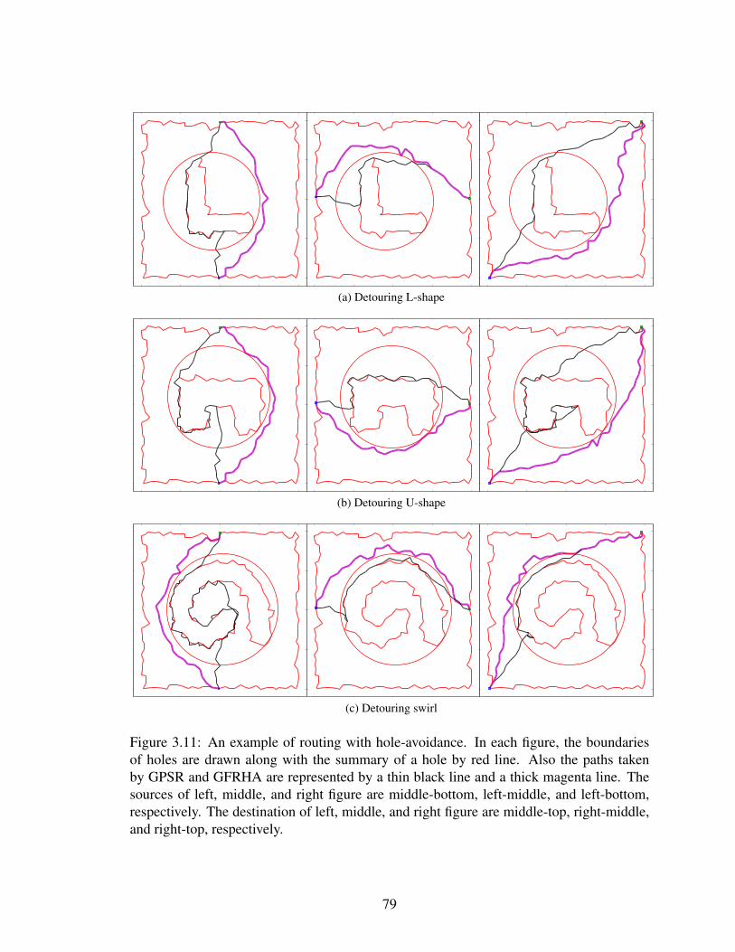
0 500 1000 1500 2000
0
500
1000
1500
2000
0 500 1000 1500 2000
0
500
1000
1500
2000
0 500 1000 1500 2000
0
500
1000
1500
2000
(a) Detouring L-shape
0 500 1000 1500 2000
0
500
1000
1500
2000
0 500 1000 1500 2000
0
500
1000
1500
2000
0 500 1000 1500 2000
0
500
1000
1500
2000
(b) Detouring U-shape
0 500 1000 1500 2000
0
500
1000
1500
2000
0 500 1000 1500 2000
0
500
1000
1500
2000
0 500 1000 1500 2000
0
500
1000
1500
2000
(c) Detouring swirl
Figure 3.11: An example of routing with hole-avoidance. In each figure, the boundariesof holes are drawn along with the summary of a hole by red line. Also the paths takenby GPSR and GFRHA are represented by a thin black line and a thick magenta line. Thesources of left, middle, and right figure are middle-bottom, left-middle, and left-bottom,respectively. The destination of left, middle, and right figure are middle-top, right-middle,and right-top, respectively.
79
ble 3.2. As shown in the table, the performance gain of GFRHA over GPSR significantly
differs depending on the shape of the hole and source and destination locations.
We also evaluate the performance comparison between GFRHA and GPSR with ran-
dom traffic. We randomly select 100 source and destination pairs from the given topologies,
where all the source and destination nodes are selected from outside of summarized holes.
Figure 3.12 shows the average path length for the random traffic when there are different
shape of holes as in Figure 3.6. Again, it is observed that the differences in path lengths
taken by GPSR and GFRHA are heavily dependent on the shape of holes. This is mainly
because the shape of a hole can significantly affect the number of hops in the perimeter
mode when a packet encounters the hole. For example, a packet can take much longer hops
to detour a hole if it is a u-shaped or a swirl-shape hole than if it is a circular-shaped hole.
On the other hand, the path length does not change much with GFRHA if the summarized
hole is similar because packets are detoured before they encounter the hole.
It is anticipated that the performance gain is greater if holes are summarized as convex
hulls, and not as circles. However, there is a trade-off between reducing energy consump-
tion in routing and disseminating hole summaries. If we use convex hulls to summarize
hole information, the data we need to disseminate the hole summary will be increased, i.e.,
we consume more energy in disseminating hole information. However, the study of such
trade-off is beyond the scope of this work. Here, we show the applicability of information
generated by TRAVERSE by other network protocols.
3.7 Conclusion
We present the TRAVERSE algorithm to identify the boundary of each hole in the de-
ployment area of sensor networks. In TRAVERSE, boundaries of holes are identifies as
follows. First, we identify candidate nodes, which are nodes that have two adjacent neigh-
bors separated more than by a predefined threshold degree. Second, we start TRAVERSE
from those candidate nodes to follow the boundaries of the holes using the right-hand rule,e
80

From mid-bottom From mid-left From left-bottomto top-bottom to mid-right to right-top
Path length Differ- Path length Differ- Path length Differ-Shape GFR- ence GFR- ence GFR- enceof hole GPSR HA (%) GPSR HA (%) GPSR HA (%)Circle 38 32 15.79 40 31 22.50 43 37 13.95Square 50 33 34.00 47 33 29.79 43 42 2.33
Rectangle 50 31 38.00 38 30 21.05 40 36 10.00L-shape 45 29 35.56 34 30 11.77 40 40 0U-shape 71 31 56.34 38 30 21.05 104 38 63.46
Swirl 137 32 76.64 43 33 23.26 49 41 16.33
Table 3.2: The path lengths taken by GPSR and GFRHA, and their differences (%). De-pending on the shape of the hole and the locations of sources and destinations, the perfor-mance gain (or loss) by GFRHA over GPSR significantly differs.
Circle Square Rectangle L U Swirl0
5
10
15
20
25
30
35
Path
length
Average path length
GPSRGFRHA
Figure 3.12: The average path length for the random source-destination pairs with differentshapes of holes.
81
with modifications for handling exceptions.
In this chapter, we show the performance of TRAVERSE both qualitatively and quanti-
tatively. We show the identification of holes with various shapes to present the qualitative
evaluation of the protocol. We also show the performance of the protocol under the realistic
log-normal shading radio model, or with the estimation errors by the localization service.
Finally, we show the application of TRAVERSE. We propose geographic forward rout-
ing with hole avoidance (GFRHA) by modifying GPSR to utilize hole information. By
utilizing hole information, GFRHA detours packets around holes before packets encounter
a hole and enter into the expensive perimeter-forwarding mode of GPSR. Evaluations show
that GFRHA can significantly reduce the path lengths depending on the shape of holes and
the locations of source and destination.
82
CHAPTER IV
ATTACK-RESILIENT COLLABORATIVE MESSAGE
AUTHENTICATION
4.1 Introduction
Data Centric Storage (DCS) [24, 27, 42, 56] is a prominent data-storage and query-
processing mechanism on Wireless Sensor Networks (WSNs). Resource-limited sensor
nodes collaboratively identify events of interest, and report them to storage nodes at prede-
fined locations according to the type of event or the range of sensed data. Queries of stored
event information can then be issued, typically by mobile users, from anywhere in the net-
work, and are forwarded to the relevant storage nodes. At storage nodes, the queries are
processed and the query results are sent back to the issuer(s). DCS is preferable to External
Storage (ES) at the base station, especially when there are many types of event to detect
and report, and not all event types are queried often in a large network [56]. Also, the time
of accessing DCS can be much shorter than that of accessing ES when storage nodes are
located close to those who need to access them. This can be achieved by replication of
storage nodes.
Security support for DCS, as for other WSN applications, is important since WSNs
usually operate in an unattended and hostile environment. Secured DCS ensures that no
fabricated information is inserted into the storage system and no unauthorized user is al-
83

lowed to access the stored data. The main challenge in securing DCS is how to verify the
authenticity of messages from remote locations since event-report, event-query and query-
response messages often need to travel multiple hops to remote nodes in a WSN.
Securing DCS, however, is very difficult, especially when attackers launch node-capture
attacks. Since sensor nodes operate in an unattended environment and may also be phys-
ically exposed to attackers, it is relatively easy for attackers to capture and then reverse-
engineer them to extract their secret (keying) information. In such a case, attackers can
subvert the entire system by compromising even a single sensor node. The attacker may
fabricate seemingly valid packets using the keying material extracted from the compro-
mised node to insert false data into the network. Depending on the type of the forged mes-
sage, the attacker may (1) report false events to storage nodes, (2) report false responses to
mobile nodes, or (3) make unauthorized accesses to the storage node by issuing queries.
Detecting forged messages is extremely difficult if they are generated using the valid
keying material, especially when they came from remote nodes. Research has been con-
ducted about the detection of data forgery using reputation systems and statistical meth-
ods [23,55,67], but the results are effective only for local data forgery, and not for messages
sent from remote nodes. Even expensive signing with public keys [46, 68] cannot handle
this problem when messages are generated using valid (stolen) keying materials. En-route
filtering mechanisms [57,71,74,80,83] provide data-forgery detection even in the presence
of compromised nodes. However, these mechanisms depend on the existence of a base sta-
tion, and cannot be applied directly to DCS, where data is sent to storage nodes at arbitrary
locations.
In this thesis, we propose Attack-Resilient Collaborative Message Authentication (AR-
CMA) to secure DCS, especially under node-capture attacks. ARCMA focuses on authen-
tication of event-report, event-query, and query-response messages that may take multiple
hops to reach their destinations. Specifically, in ARCMA, a set of sensor nodes cooperate
to evaluate a Collaborative Message Authentication Code (CMAC) for the messages sent
84
to, and received from, remote nodes. As a traditional MAC, a CMAC is evaluated both at
the sender and the receiver sides, and only those messages with valid CMACs are accepted
by the receiver. Since the keying material of sensor nodes may be exposed under node-
capture attacks, sensor nodes must collaborate to provide necessary protection against such
attacks. This is akin to the sensor nodes’ collaboration (to overcome their limitations in
sensing capability) to identify the events of interest to the underlying applications.
The main contributions of this work are summarized as follows. First, we propose a
novel attack-resilient message authentication mechanism, called ARCMA, in which each
node belongs to one of k groups, and a message is collaboratively authenticated and ver-
ified by k nodes, each from a distinct group. To achieve this, each node maintains an
Authentication Tree (AT), which is a spanning tree formed with k nodes, each from one of
k distinct groups, and collaborates with all the nodes in its AT to evaluate CMAC for mes-
sage authentication. We also encrypt messages with location-dependent keys to validate
their origin.
Second, we show how ARCMA can be applied to authenticate messages associated with
DCS operations. We show how each parameter can be set for (1) event-report messages
which are typically generated by a set of cooperating sensor nodes in proximity, (2) event-
query messages which are generated by mobile users, and (3) query-response messages
which are sent back to the mobile users. Most previous work focused on securing event-
report messages destined for the base station, and does not consider how to secure the
processing of queries issued by mobile users.
Third, we present heuristics to construct ATs and to assign sensor nodes to different
groups. Since a global view is not available, or too expensive to obtain in a WSN, we
propose two distributed heuristic algorithms to build ATs, MIN and OPT. We also provide a
group-assignment protocol, in which sensor nodes in the neighborhood assign their groups
such that different group numbers can be assigned.
Finally, we analyze the security of ARCMA and evaluate its performance. We show that
85
the security of ARCMA does not degrade as long as less than k nodes are compromised.
Also, we evaluate the overhead of constructing ATs and exchanging extra messages for
message authentication for design parameter k and node density.
The rest of this chapter is organized as follows. The related work is summarized in
Section 4.2. Section 4.3 describes the system model and assumptions used throughout the
chapter, and the key management for the proposed protocol is described in Section 4.4.
Then, ARCMA is detailed in Section 4.5, followed by descriptions of the authentication-
tree construction in Section 4.6 and group assignment in Section 4.7. Section 4.8 presents
the security analysis and the performance evaluation of ARCMA. Section 4.9 concludes
this chapter.
4.2 Related Work
DCS [24, 27, 42, 56] was proposed to store and query the information (e.g., events of
interest) collected in a WSN. The events of interest detected by the WSN or their metadata
are reported to storage nodes whose locations are pre-determined based on the type or range
of the sensed data, and queries for this information are delivered to, and processed at those
storage nodes.
Various key management protocols have been proposed to support the security of WSN
applications. Key management in a WSN is a challenging problem due to the large network
size and the severe resource limitation in each node. For symmetric key sharing, several
key pre-distribution schemes [13, 14, 17, 32, 44] have been proposed that assign a partial
set of keys or keying material to each sensor node so that each pair of neighboring nodes
can establish a shared key with a high probability. TinyPK [68] and ECDLP [46] are the
implementations of public-key cryptography for WSNs.
However, the security of DCS cannot be achieved by just encrypting/signing messages
with the keys generated by the above key management protocols. In DCS, event-report and
event-query messages typically take multiple hops to reach remote storage nodes. Thus,
86

the securing DCS requires authenticating these messages. However, node-capture attacks
are relatively easy to mount in WSNs, and an insider attack using the keying material
extracted from the captured nodes can be catastrophic if the attacker can generate any event-
report, event-query, or query-response message. In such a case, all of the above-mentioned
schemes will become futile.
R-DCS [25] replicates storage nodes for scalability and resilience, but it cannot tolerate
active attacks including node-capture attacks. pDCS [60] provides security and privacy on
DCS by using a keyed hash function to map the storage nodes, but it cannot also prevent
fabricated event-reports after node-capture attacks.
Several protocols have been suggested to provide secure event reports under node-
capture attacks. Secure aggregation [55, 67] and en-route filtering [5, 57, 71, 73, 83] are
suggested to prevent the reporting of invalid information only to an uncompromisable base
station, and the base station has all the keying material to validate any packet. In these
protocols, each sensor node has either a pairwise key with the base station or a set of keys
randomly selected from a large key pool. On the other hand, the base station has either pair-
wise key with all the sensor nodes, or all the keys from the key pool. When sending event
information, a sensor node authenticates the event message with one of the keys it has. In
en-route filtering, such event messages can be statistically filtered when they are invalid; a
forwarding node may verify the messages if it has the same key used for authenticating the
messages. Since a sensor node has only a subset of the key pool, it may be possible that
an invalid packet may be forwarded to the base station. Thus, the final verification of the
event messages should be handled by the base station. These protocols are not applicable
to DCS, where any easily-attacked sensor node should be able to receive and verify event
messages as a storage node. If each sensor node has all the keying material to validate any
incoming packet, it is equivalent to having one common key shared by every node. In this
case, the whole system is subverted when only one node is compromised.
A reputation-based system such as [23] was proposed to detect the reporting of false
87
information. In such a system, the reputation of a sensor node is determined by its be-
haviour that is monitored by other sensor nodes. If the reputation of a certain sensor node
is below a threshold, the node is ignored by other nodes. For example, other nodes do
not forward packets originating from low-reputation nodes. In such a system, if the rep-
utation of a sensor node is maintained only locally, an attacker may insert invalid packets
by compromising only one node and moving to a new location after the reputation of the
compromised node becomes lower than the threshold. To share a reputation of a sensor
node globally, the reputation of a specific node should be stored in a predefined location,
e.g., the location of the reputation storage can be evaluated using a hash function as the
location of storage nodes is determined in DCS. However, securing such reputation update
is not trivial, and such updates are too expensive for battery-powered and low-bandwidth
sensor nodes. Also, reputation systems proposed for sensor networks [23] assume that each
sensor node verifies the messages generated by its neighbors in a promiscuous mode, and
build each other’s reputation. However, wireless links are typically asymmetric, and thus,
a node cannot always hear all of its neighbors. Also, the requirement that every message
should be interpretable by intermediate nodes between the source and the destination may
create security holes. That is, a message’s content may be exposed to the attacker if one of
the nodes on its path was compromised.
Zhang et al. [79] proposed a countermeasure against node-capture attacks on mobile
sinks. Their solution focused on an application scenario in which mobile sinks are used to
retrieve the sensed data, and their main goal is to prevent unauthorized data access via a
compromised mobile sink, not compromised sensor nodes. They allow the least privilege
to a mobile sink such that it can access the authorized information. To do so, they assumed
the existence of an uncompromisable and resourceful base station, which has a pairwise
key to every sensor node. The base station provides mobile sinks with security credentials,
which can be verified by sensor nodes using their keys shared with the base station.
ARCMA differs from the above approaches in that it can authenticate messages sent to
88
any other locations, and it does not assume any uncompromisable base station. Besides,
ARCMA provides k-collusion resistance, i.e., the security of the system does not degrade
if less than k nodes are compromised, like most of the secure aggregation or en-route
filtering [5, 57, 73, 83].
4.3 System Model
4.3.1 Sensor Network Model
DCS is placed on a WSN, which is usually composed of a large number of inexpen-
sive sensor nodes with limited memory, computation and communication capacities. Sen-
sor nodes are usually battery-powered, and hence, energy is a precious, scarce resource.
Hardware-supported tamper-proofing is usually not a feasible solution for sensor nodes
due to its higher hardware cost.
We assume sensor nodes to have been deployed densely such that events of interest
can be detected by a set of cooperating sensor nodes near the locations of their occurrence.
More specifically, we require a network dense enough so that an event can be detected by at
least k nodes. The conditions of network-density and relevant sleep-scheduling algorithm
for this requirement is discussed in [36]. There are other compelling reasons for dense
deployment, such as fault-tolerance and short-range communication. Detected events will
be sent to (possibly remote) storage nodes, where information about the event is stored
or possibly aggregated with other information. The storage nodes are nothing but sensor
nodes, which are selected a priori according to a pre-defined rule. An event-report message
may traverse a large number of hops if the storage nodes are located far away from its
occurrence.
External mobile nodes, which may be carried by users or attached to ground/air vehi-
cles, may interact with nearby sensor nodes, issuing queries for the information of interest.
Sensor nodes will forward the queries issued by mobile nodes to the storage nodes that will
89

then reply with the queried information. The mobile nodes usually have more (computa-
tion, communication and energy) resources than sensor nodes.
The existence of a base station is not assumed in ARCMA as in many other works [5,
55, 57, 67, 71, 73, 79, 83]. Using a base station as a trusted third party, solutions to many
security problems can be simplified. However, adoption of a base station has the following
problems. First, it is not always guaranteed to have stable communication to a base station.
Second, it may be expensive to communicate with a base station since it can be located
far from most of deployed sensor nodes. For example, DCS is more efficient than ES
using a base station in terms of the communication cost when there are many event types
and frequent queries [56]. Finally, a base station can be the single point of failure. If the
base station of a deployed network is faulty or compromised, the whole system would not
function. Thus, in the previous work, the existence of an uncompromisable base station is
assumed. In ARCMA, we did not assume the existence of a base station at all.
In designing ARCMA, we assume existence of the following three common services:
localization [8,30,38,59], time synchronization [16,22,63,64], and geographic forwarding
routing [7,33]. All of these services are basic and usually required for other sensor network
applications than DCS; localization and time-synchronization services are required to pro-
vide the location and the time of each identified event, and geographic forwarding routing
is required to forward event-report and query messages. ARCMA exploits these “already
available” services without incurring additional costs.
4.3.2 Attack Models
WSNs are inherently vulnerable to various security attacks because they usually operate
in an unattended and hostile environment. We assume that attackers are resourceful and mo-
bile, and launch several types of attacks. Attackers can launch outsider or insider attacks.
An outsider attack may be passive such as eavesdropping communications or performing
traffic analysis, or active such as inserting, modifying, or dropping packets. Adversaries
90

can launch a stronger type of (insider) attack, such as node-capture attacks in which sen-
sor nodes are captured and compromised to extract their keying material. A node-capture
attack is relatively easy to mount in WSNs since sensor nodes operate in an unattended
environment, and are therefore likely to be exposed to attackers. The main focus of this
chapter is to secure DCS against node-capture attacks.
We assume that attackers of DCS want to (1) disable the targeted DCS by inserting
false data so that the legitimate users will receive incorrect data, (2) report false data to
the legitimate query issuers, or (3) access the stored data for unauthorized purposes. An
attacker can achieve all of these goals by inserting false messages into the system. For
example, if an attacker can generate valid-looking, i.e., generated with valid keys, event-
report messages so that the false event information is stored at the storage nodes, all the
users who issue queries will receive the false event information. Similarly, the attacker can
report false data to queries or access stored data by inserting false messages.
The proposed protocol in this work, therefore, focuses on preventing an attacker from
inserting false messages into the system. In the proposed protocol, we guarantee that at-
tackers cannot insert any false message, i.e., the security does not degrade, as long as less
than k nodes are compromised.
Also, even when k or more than k nodes are compromised, to generate a false message
originating from a certain area, the attacker has to compromise at least one node from k
different areas. This fact limits the attackers’ ability to insert false messages. For example,
an attacker cannot forge an event-report message from a certain area if he does not com-
promise at least one node from the area unless he compromises k nodes from different k
areas.
We, however, assume that the network is safe for a short while after the deployment,
during which the initialization can be performed. This is realistic, since it takes time for
attackers to learn the existence and operation of a WSN, and to compromise sensor nodes.
91
4.4 Key Management
In this section, we present a key management that adopts polynomial-based key pre-
distribution for the proposed protocol. The polynomial-based key pre-distribution is adopted
since its security does not degrade if less than a certain number of nodes are compromised.
This means that an attacker does not obtain any information of the polynomial if the number
of compromised nodes is below a threshold.
4.4.1 Polynomial-based Key Pre-distribution
We first summarize polynomial-based key pre-distribution [6], on which the key man-
agement of ARCMA relies.
A (k−1)-degree1 bivariate polynomial is defined as
f(u, v) =k−1∑i,j=0
aijuivj
over a finite field Fq, where q is a prime number large enough to accommodate a crypto-
graphic key. When a bivariate polynomial is symmetric (i.e., f(u, v) = f(v, u)), we define
a share of the polynomial of node s as f(s, v), which is a (k−1)-degree univariate polyno-
mial. By distributing a share of the polynomial to every sensor node, any two nodes in the
network can set up a pairwise secret by exchanging only their node IDs. For example, two
nodes s and r share a secret by replacing the variable of their share of the polynomial with
the correspondent’s ID, i.e., f(s, r) = f(r, s). The common secret between any two nodes
is proven to be safe if less than k shares of the (k−1)-degree polynomials are revealed to
the adversary, i.e., less than k nodes are compromised.
1We use (k−1)-degree polynomials instead of k-degree polynomials as in most literature to simplifynotations in the later sections.
92
4.4.2 Key Distribution
ARCMA uses three sets of bivariate polynomials to generate keys for different pur-
poses: pairwise-key, group-key, and spatial-key polynomials.
1. Pairwise-Key Polynomial, fp(u, v): is used to generate the pairwise key between any
two sensor nodes in the neighborhood, or between a mobile node and a sensor node.
Each polynomial variables will be replaced by the node ID.
2. Group-Key Polynomial, fg(u, v): is used to evaluate the MACs of messages. One
variable of the group-key polynomial will be replaced by group number, and the other
by the node ID. To prevent the collusion attack since the polynomial is commutative,
we set the mobiles’ ID greater than k.
3. Spatial-Key Polynomial, fs(u, v): is used to generate encryption-keys for messages
forwarded to remote locations. Since the destinations of such messages are speci-
fied as their location (not ID) in DCS, the variables are replaced with the location
information of the sender and the receiver of a given message.
When sensor nodes are deployed, they are preloaded with a common master key K0.
The coefficients of the above three-polynomials are derived from this key using the com-
mon keyed hash function HK(). The coefficient aij of fp are evaluated as
aij =
HK0(i · k + j +B) if i ≤ j
aji otherwise
where B is set to 0. By setting B to k2 and 2 · k2, the coefficients of two other polynomials
fg and fs are evaluated.
The master key K0 will be permanently removed from the memory of sensor nodes
after evaluating coefficients of the polynomials.
93

4.4.3 Key Assignment
Once deployed, sensor nodes evaluate their share of pairwise-key polynomial by replac-
ing one of the variable with their own ID. Then, they discover their one-hop neighbors, and
establish pairwise keys with them. Each sensor node broadcasts its own ID, and the pair-
wise key can be simply evaluated using the pairwise-key polynomial using the neighbor’s
ID.
After discovering its neighbor nodes, each sensor node generates a random number that
is used for the cluster key. The cluster key of a node is used to encrypt local broadcast
messages sent by a specific node. The cluster key can be encrypted with the pairwise key
and delivered to all neighbors individually. Let CKs be the cluster key of sensor node s.
Once local relations are secured, the underlying localization protocol can be evoked.
The pairwise keys and cluster keys established in the above process may be used to encrypt
or decrypt messages of the localization protocol, if necessary. After the location of each
sensor node is discovered through the localization service, each sensor node evaluates its
share of spatial-key polynomial.
When evaluating the spatial-key polynomial, quantized coordinates are used instead of
the raw coordinates. Since the exact coordinates of remote nodes are, in general, not known
a priori, the exact coordinates of the destination cannot be used with the spatial-key poly-
nomial to obtain a matching key both at the source and the destination. (In the geographic
forwarding routing, knowledge of the exact coordinates are not necessary since a packet is
handled by the sensor node that is the closest to the destination.) Thus, we use the quan-
tized coordinates, and the spatial-key is associated with the quantized coordinates, rather
than the exact geographic location. The quantized location (Ls) of a sensor s located at
(x, y) is defined as Ls = b x`0c|b y
`0c. Here, the quantization index `0 determines the gran-
ularity of the quantization. Then, s’s share of the spatial-key polynomial can be evaluated
to be fs(Ls, v). The use of the quantized coordinates is equivalent to dividing the whole
network area into squares whose edge length is `0, and the lower-left corner of a grid is
94
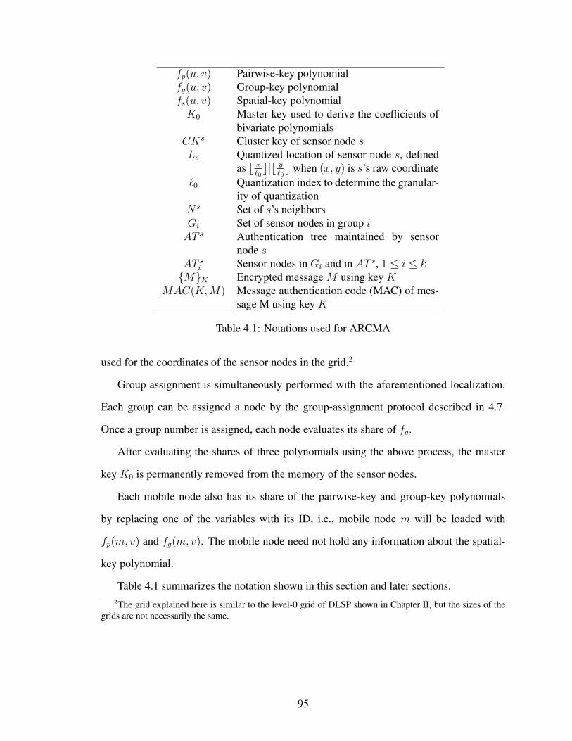
fp(u, v) Pairwise-key polynomialfg(u, v) Group-key polynomialfs(u, v) Spatial-key polynomialK0 Master key used to derive the coefficients of
bivariate polynomialsCKs Cluster key of sensor node sLs Quantized location of sensor node s, defined
as b x`0c|b y
`0c when (x, y) is s’s raw coordinate
`0 Quantization index to determine the granular-ity of quantization
N s Set of s’s neighborsGi Set of sensor nodes in group iAT s Authentication tree maintained by sensor
node sAT si Sensor nodes in Gi and in AT s, 1 ≤ i ≤ k{M}K Encrypted message M using key K
MAC(K,M) Message authentication code (MAC) of mes-sage M using key K
Table 4.1: Notations used for ARCMA
used for the coordinates of the sensor nodes in the grid.2
Group assignment is simultaneously performed with the aforementioned localization.
Each group can be assigned a node by the group-assignment protocol described in 4.7.
Once a group number is assigned, each node evaluates its share of fg.
After evaluating the shares of three polynomials using the above process, the master
key K0 is permanently removed from the memory of the sensor nodes.
Each mobile node also has its share of the pairwise-key and group-key polynomials
by replacing one of the variables with its ID, i.e., mobile node m will be loaded with
fp(m, v) and fg(m, v). The mobile node need not hold any information about the spatial-
key polynomial.
Table 4.1 summarizes the notation shown in this section and later sections.2The grid explained here is similar to the level-0 grid of DLSP shown in Chapter II, but the sizes of the
grids are not necessarily the same.
95

4.5 Attack-Resilient Collaborative Message Authentication (ARCMA)
4.5.1 Overview
In ARCMA, sensor nodes collaboratively authenticate messages sent to, and received
from, remote nodes. The traditional message-authentication method relies on MAC, which
is evaluated as a one-way keyed hash function. However, this method is not sufficient for
WSNs because it is relatively easy for the adversary to capture nodes on WSNs. With
valid keying materials extracted from the captured nodes, the adversary can then insert a
message with a valid MAC. To prevent such attacks, ARCMA requires messages to be
authenticated collaboratively by a set of sensor nodes. More specifically, each sensor node
belongs to one and only one of k distinct groups, and members of each group share a
group-key polynomial to generate a common key to evaluate MACs. When authenticating
a message, k nodes from k distinct groups, one from each group, evaluate MACs using
group-keys, and the CMAC is evaluated by XORing these MACs. Like a traditional MAC,
the CMAC is evaluated at the sender side and concatenated to the message. Then, the
CMAC is re-evaluated at the receiver side for its verification. Using CMACs, messages
can be authenticated even under node-capture attacks since the attacker must know all k
group keys to fabricate a valid MAC.
To evaluate a CMAC, each sensor node needs to know at least one node for each of
k groups in its neighborhood. Thus, each node maintains an AT, a structure to maintain
information on nodes for each of k groups. AT is a spanning tree with at least k nodes.
Using its AT, a sensor node can evaluate or verify the CMAC. For convenience, the AT
maintained by node s is represented by AT s, and sensor nodes in AT s are represented as
AT si , where i is the group the node belongs to. Each sensor s node maintains the following
information in its AT: the node ID for AT si , the next hop to AT si , and the number of hops
to AT si for each group i (1 ≤ i ≤ k).
Figure 4.1 shows an example of ATs. Figure 4.1(a) depicts a given topology, where
96

61
22
11
33
83
55
94
72
44
(a) An example topology. Vertices and edges repre-sent nodes and connectivity between nodes, respec-tively. The main number and the subscripted num-ber in a vertex represent the ID and group numberof the node, respectively.
61
22
11
33
83
55
94
(b) A (possible) authentication treefor node 1.
11
33
55
72
44
(c) Another possible authenti-cation tree for node 1.
Figure 4.1: Example of authentication trees: This figure shows ATs in a given topologywhen k = 5
vertices and edges represent nodes and connectivity, respectively. The ‘main’ number and
the number in parentheses in a vertex represent the node ID and its group number when
k = 5. Figures 4.1(b) and 4.1(c) show possible AT 1.
4.5.2 Collaborative Message Authentication
We now describe how messages are exchanged when sensor node s located in Ls sends
a message M to anther sensor node r located in Lr. In summary, s computes a CMAC
for M and encrypts them with a proper spatial-key. When r receives M , it evaluates the
CMAC after decrypting it, and checks if the evaluated CMAC and the received CMAC
match. It accepts the message only when the two CMACs match.
Messages at the sender’s side are exchanged as follows.
1. s sendsM to the nodes inAT s. s sendsM with ID id, timestamp ts, and its location,
Ls, to all the nodes in its AT. Here, id is a parameter other than group number for
the group-key polynomial, the timestamp is used to prevent replay attacks, and the
97

location is used to provide the authenticity of the location of reported data. PM is
a proof of message which is used to prevent the compromised node from asking
the message authentication for forged messages. Depending on the type of a given
message, these fields will be filled in with different values. This will be detailed
in Section 4.5.3.
s→ AT si : {id|M |ts|Ls|PM}fp(s,AT si ) for 1 ≤ i ≤ k
2. s receives MACs evaluated by the nodes in AT s. The nodes in AT s evaluate the
MAC for the given message with the timestamp and the location of s, and then return
it to s. Note that this is processed only when a valid proof PM for the given message
M is provided.
AT si → s : {MAC(fg(i, id),M |ts|Ls)}fp(s,AT si )
3. s computes the CMAC by XORing the MACs it received. s evaluates a CMAC as
follows:
CMAC = MAC(fg(1, id),M |ts|Ls)⊕
MAC(fg(2, id),M |ts|Ls)⊕ · · · ⊕
MAC(fg(k, id),M |ts|Ls).
4. s encrypts M with its spatial key, and sends it to r. s concatenates the timestamp, its
location and CMAC to the message, and sends the concatenated message to r using
the underlying routing protocol.
98
s→ r : Ls, Lr, {M |ts|Ls|CMAC}fs(Ls,Lr)
When r receives the message, it evaluates the CMAC using its own AT, similarly to the
CMAC evaluation at the sender side, as follows.
1. r sends M to the nodes in AT r. r decrypts the message with fs(Ls, Lr), and sends it
to the nodes in its AT. Here, the proof of message is not required since r’s location is
different from s’s location, Ls.
r → AT ri : {id|M |ts|Ls}fp(r,AT ri ) for 1 ≤ i ≤ k
2. r receives the MACs evaluated by the nodes in AT r. When the nodes in r’s authenti-
cation tree, AT r, receive the message, they evaluate the MAC for the given message
with the group-key and return it to r.
AT ri → r : {MAC(fg(i, id),M |ts|Ls)}fp(r,AT ri )
3. r evaluates the CMAC and accepts the message only if CMACs match. Upon re-
ceiving replies from the nodes in AT r, r evaluates the CMAC for the given message
by XORing the received MACs. Only if the CMAC from s matches the CMAC it
computed, will r accept the message.
In the above process, the same message M is transmitted to all the nodes in AT s and
AT r. This will be very expensive, thus calling for an optimization to reduce the number of
message transmissions. Without optimization, the cost of exchanging messages to evaluate
the CMAC increases linearly with k. However, we need not send the same message to all
the nodes individually, since the message is known to the local nodes. So, we can use a
local broadcast using s’s cluster key, CKs. If a node needs to forward such a message
99

asking for MAC, i.e., it has child node(s) in AT s, it can again send the message using its
own cluster key. When MACs are received, the intermediate nodes in a node’s AT can XOR
all the MACs it receives from its children, and then report the XORed MAC to its parents.
When s receives such reports from its children, it can compute the CMAC by XORing
them. The CMAC obtained from this optimization will be the same as that obtained by
XORing individual MACs at s since XOR is transitive. When the CMAC is verified by r,
a similar step can be taken.
A CMAC mismatch indicates a compromise. If the CMAC computed by r does not
match the CMAC from s, at least one node in either AT r or AT s did not report a proper
MAC. In such a case, r can send the same message M to all the nodes in AT r individually
without optimization. Then, r can send all of the MACs to s. Upon receiving such a
message, s also requests nodes in AT s to re-evaluate the MACs. If the MACs for a certain
group do not match, either the nodes of a group in AT s or AT r, or both, are compromised.
In such a case, both nodes are revoked. This revocation process is expensive since the same
message should be sent to all the nodes in AT s and AT r. However, this type of attack is
not effective from an attacker’s standpoint not only because the attack is easily detectable
but also because the compromised nodes are revoked upon their first attack.
4.5.3 Securing DCS Operations Using ARCMA
We now describe how ARCMA can be used for securing DCS messages: event-report,
event-query, and query-response messages. Regardless of message types, messages are
transmitted to remote locations. So, the collaborative authentication described in the previ-
ous subsection can be used. However, different proofs of messages for CMAC evaluation
are required for different types of messages.
100

4.5.3.1 Reporting Sensed Data
Sensor nodes cooperate to identify events of interest; an event will typically be de-
tected by multiple sensor nodes, and their sensor readings will be aggregated for detection
accuracy.
When such an event is reported to the corresponding storage nodes, the report message
must be authenticated to guarantee the authenticity of the report. ARCMA can be used for
this purpose, and the information about the event can be used as the proof of the message.
Node density in a WSN is determined so that any region is covered by more than a certain
number of nodes [36] for an event of interest to be detected with a desired level of accuracy
since each sensor node has only limited sensing capability. By adjusting the sensor node
density, we can, therefore, make an event detectable by at least k nodes which can partic-
ipate in authenticating the event to be reported to the corresponding storage node. These
nodes evaluate MAC only when the information in the event-report message is consistent
with the information they have, i.e., they use the information about the event as a proof of
the message. The id field of ARCMA messages is filled with the ID of the sensor node that
composes the event-report message.
The storage node verifies the authenticity of each event-report message using its own
AT, and stores only validated messages. Once verified, the reported event is stored by all
the k nodes in the receiver’s authentication tree as replicas. These replicas are later used as
the proof of message for query-response messages.
4.5.3.2 Processing Queries Issued by Mobile Users
An external mobile user may query the sensor network to retrieve the data stored in
DCS. Such queries are routed via multiple hops to the storage nodes, and then the corre-
sponding results are generated and sent back to the mobile user. In this scenario, both the
query and the result should be verifiable.
A valid query should be generated only by a legitimate mobile user. So, a mobile user
101

should be authenticated first before issuing queries to the network. However, it should be
authenticated by multiple nodes rather than just by one node. When authenticated, the
mobile user will be issued a token, which is a security credential it can present to the
sensor nodes that belong to the same group as the token-issuer. After collecting k tokens,
the mobile user can issue a query by presenting tokens as the proof of event-query, i.e., the
query is validated by the security credentials issued by k different sensor nodes.
Mobile node m can be authenticated by sensor node s by exchanging three-way hand-
shakes. First, m sends s its ID and a nonce, Nm. When s receives such a message, it also
generates a nonce, Ns. Then, s sends its own ID along with Nm and Ns after encrypting
it with a pairwise key between s and m, fp(s,m). Note that both s and m can evaluate
the pairwise key using the pairwise-polynomial after exchanging their IDs. Then, m sends
the nonce generated by s after encrypting it with fp(s,m). Now, s and m can mutually
authenticate each other.
m→ s : m,Nm
s→ m : s, {Ns|Nm}fp(s,m)
m→ s : {Ns}fp(s,m)
Then, s sends m a token, Tg(m), if it belongs to group g. Tg(m) is defined as
Tg(m) ≡ s|g|m|ts|{s|g|m|ts}fg(g,m)
This token is valid only to the nodes in group g, and only m can present this token to
the sensor nodes since only m can evaluate the pairwise-keys with arbitrary sensor nodes.
Here, ts is a timestamp to indicate the time when the token is issued, and may be used by
sensor nodes to reject stale tokens.
102

s→ m : Tg(m)
Whenm needs to issue a query, Q, it sends a query message to one of the nearby sensor
nodes with the k tokens it has collected as the proof of message. Also, it evaluates CMAC
for the query which can be evaluated with its share of the group-key polynomial. Here,
CMAC is evaluated with the timestamp of the current time and the location of s. CMAC
is evaluated by the mobile user to reduce the overhead of sending an invalid query. A
legitimate mobile user can evaluate CMAC, and there is no reason for it to generate an
invalid CMAC.
m→ s : ts|Ls|{Q|ts|Ls|CMAC}fp(m,i)|Tg(M)
where 1 ≤ g ≤ k, and CMAC ≡ MAC(fg(m, 1), Q) ⊕ MAC(fg(m, 2), Q) ⊕ · · · ⊕
MAC(fg(m, k), Q).
Then, s sends tokens and collects MAC for the given query, Q.
s→ AT si : {Q|ts|Ls|Tg(m)}fp(s,AT si ), where 1 ≤ i ≤ k
The nodes in AT s verify the token, which is the proof of the event-query message, and
send s either MAC for the query message or INVALID message.
AT si → s : {MAC(fg(m, i), Q|ts|Ls)}fp(s,AT si ) or INVALID.
If all the tokens are valid, s can evaluate CMAC by XORing MACs it has collected.
Then, it checks if the evaluated CMAC and the CMAC received from the mobile user
match. Only when they match, does s send the query, Q, to the storage nodes.
When the query is received by r, which is a storage node, it first verifies the message
using AT r; then r composes the query-response, R, for the valid query. The reply message
103

is again authenticated using AT r, and the query-response message R itself is used as the
proof of message; all k nodes should store the same event as a replica of the event, and
they verify R by comparing it with the stored events. Then, the query-response message
is encrypted with the pairwise-key between r and m, fp(r,m); the encrypted message
is evaluated using the pairwise-key polynomial so that the clear text of message is only
readable by m.
r → m : r, {R|ts|Lr|CMAC}fp(r,m)
When m, the query issuer, receives this message, it evaluates CMAC using its share of
the group-key polynomial, and accepts it only when a valid CMAC is concatenated to the
reply message.
4.6 Authentication Tree Construction
Since a global view is not available at any given sensor node, we present two simple
heuristic algorithms to construct ATs without incurring high overhead. The first heuristic,
called MIN, builds a minimum-depth tree by selecting the shortest-distance node from a
certain group for the AT. This heuristic adds a small amount of information in a periodic
beacon message, commonly used in sensor network applications like health monitoring,
node discovery, and route discovery. In each periodic beacon message, a node advertises
the groups it has discovered by using a k-bit vector. When a sensor node notices that
some bits are not set in a neighbor’s beacon while the corresponding bits are set in its own
bit vector, i.e., its neighbor has not yet discovered the nodes in certain groups that it has
already discovered, it announces the information about them in its next beacon message.
When a sensor node detects such information in its neighbor’s beacon, it updates its AT.
Using these steps, a t-hops-away node can be discovered within t beacon periods, as in a
distance-vector routing protocol. The pseudo-code of this heuristic is given in Algorithm 1.
104
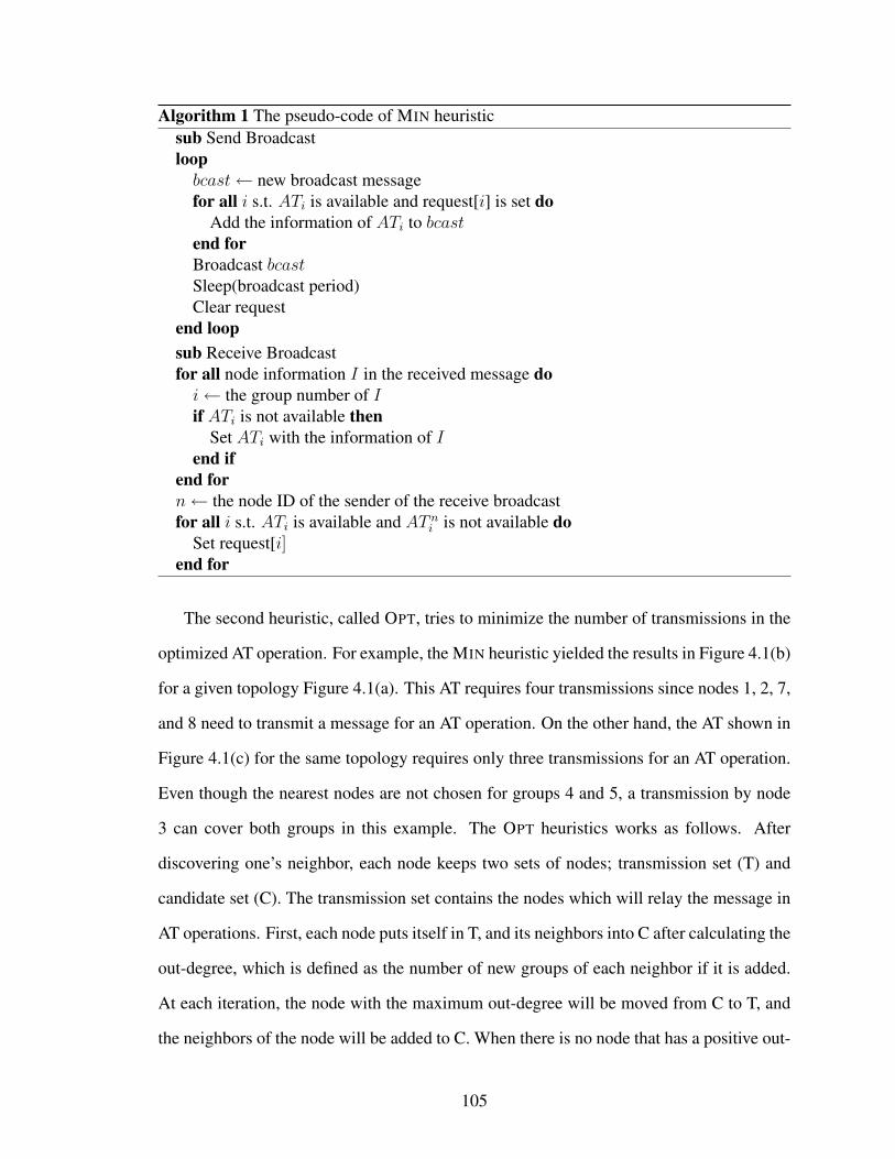
Algorithm 1 The pseudo-code of MIN heuristicsub Send Broadcastloopbcast← new broadcast messagefor all i s.t. ATi is available and request[i] is set do
Add the information of ATi to bcastend forBroadcast bcastSleep(broadcast period)Clear request
end loopsub Receive Broadcastfor all node information I in the received message doi← the group number of Iif ATi is not available then
Set ATi with the information of Iend if
end forn← the node ID of the sender of the receive broadcastfor all i s.t. ATi is available and AT ni is not available do
Set request[i]end for
The second heuristic, called OPT, tries to minimize the number of transmissions in the
optimized AT operation. For example, the MIN heuristic yielded the results in Figure 4.1(b)
for a given topology Figure 4.1(a). This AT requires four transmissions since nodes 1, 2, 7,
and 8 need to transmit a message for an AT operation. On the other hand, the AT shown in
Figure 4.1(c) for the same topology requires only three transmissions for an AT operation.
Even though the nearest nodes are not chosen for groups 4 and 5, a transmission by node
3 can cover both groups in this example. The OPT heuristics works as follows. After
discovering one’s neighbor, each node keeps two sets of nodes; transmission set (T) and
candidate set (C). The transmission set contains the nodes which will relay the message in
AT operations. First, each node puts itself in T, and its neighbors into C after calculating the
out-degree, which is defined as the number of new groups of each neighbor if it is added.
At each iteration, the node with the maximum out-degree will be moved from C to T, and
the neighbors of the node will be added to C. When there is no node that has a positive out-
105
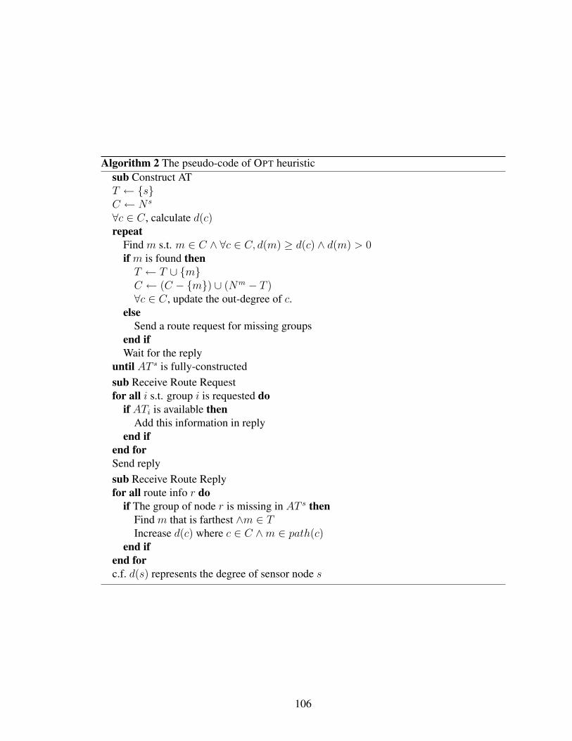
Algorithm 2 The pseudo-code of OPT heuristicsub Construct ATT ← {s}C ← N s
∀c ∈ C, calculate d(c)repeat
Find m s.t. m ∈ C ∧ ∀c ∈ C, d(m) ≥ d(c) ∧ d(m) > 0if m is found thenT ← T ∪ {m}C ← (C − {m}) ∪ (Nm − T )∀c ∈ C, update the out-degree of c.
elseSend a route request for missing groups
end ifWait for the reply
until AT s is fully-constructedsub Receive Route Requestfor all i s.t. group i is requested do
if ATi is available thenAdd this information in reply
end ifend forSend replysub Receive Route Replyfor all route info r do
if The group of node r is missing in AT s thenFind m that is farthest ∧m ∈ TIncrease d(c) where c ∈ C ∧m ∈ path(c)
end ifend forc.f. d(s) represents the degree of sensor node s
106

degree in C, a sensor node will request the route for the missing groups. Upon receiving
such a request, a sensor node replies if it has access to the group. The pseudo-code for this
heuristic is given in Algorithm 2.
4.7 Group Assignment Protocol
Group assignments of sensor nodes significantly affect the functionality and perfor-
mance of ARCMA, where one node from each of k groups should collaborate together.
Thus, the group assignment should guarantee uniform distribution of groups across the
deployment area.
In ARCMA, groups can be distributively assigned at each grid. A sensor node deter-
mines its quantized coordinates, i.e., the grid it belongs to after it obtains its geographic
location and deployment area information through a localization service. Then, sensor
nodes in a grid discover each other by exchanging their own IDs and their neighbors’ IDs
within the grid. After that, the node with the smallest node ID in the grid assigns groups to
sensor nodes. In doing so, it can uniformly assign group numbers to sensor nodes. More
specifically, if there are i · k + j nodes in the grid, where i ≥ 0 and 0 ≤ j < k, the sensor
nodes with minimum ID assigns at least i nodes to each of k groups. When there are less
than k nodes in the grid, sensor nodes in the grid will have limited capability to send or
receive authenticated messages; they may find sensor nodes from the missing groups in the
neighbor grids. However, an event-report message may not be authenticated in the grid
when less than k nodes observe a given event.
4.8 Evaluation
4.8.1 Security Analysis
We analyze the security of ARCMA against the various attacks described in Section 4.3.2.
Since all the messages are encrypted with the relevant keys, the proposed protocol is safe
107

from passive or active outsider attacks as long as proven cryptography is used. Also, replay
attacks are prevented since all the messages including tickets contain time-stamps. Thus,
our analysis will focus on node-capture attacks, where valid keying materials are exposed
to attackers.
Also, ID spoofing and Sybil attacks can be prevented by using the bivariate polynomi-
als. Without knowledge of the pairwise-key polynomial, the attacker cannot generate the
secret keys for the spoofed IDs. Therefore, the attacker cannot launch a Sybil attack with
spoofed IDs.
Now we focus on security analysis when an attacker launches node-capture attacks. In
this case, the attacker has the valid keying information so that the naive encryption will
not prevent the attacker from inserting false messages. We first consider the case where the
attacker compromises less than k nodes, and then, the case where the attacker compromises
k or more nodes.
When less than k nodes are compromised: Let us consider the case where the attacker
compromises less than k nodes. In such a case, the attacker has the full control of the
compromised nodes and the full knowledge of the keying material in the nodes. Using
these keying materials, the attacker can launch different attacks depending on how the
compromised nodes are used in the system.
There are a few options that the attacker can choose with the compromised nodes. The
first option is to stay silent when the compromised nodes are asked to evaluate a MAC
by a certain node which has the compromised nodes in its AT. The second option for the
attacker is to report a wrong MACs when the compromised nodes are asked to evaluate
a MAC. Another option for the attacker is to try to generate a message by asking other
nodes to evaluate MACs to compose a false message. This type of attack will be the most
attractive to the attacker since the attacker can generate any message to subvert the system.
For example, the attacker may generate event-report messages to report false events, or
event-query messages to retrieve detected events. Here we discuss how ARCMA prevents
108

such attacks.
Lemma IV.1. The security of ARCMA does not degrade, i.e., the integrity of the system
remains the same if less than k compromised nodes remain silent when requested for MAC
evaluation.
Proof. Here, the requesting node may be either a sender or a receiver. In this case, the re-
questing node can wait for the time being, and after a timeout, it can consider that the nodes
are dead and recruit other nodes from the group where the compromised nodes belong, us-
ing the reconstruct algorithm. Note that for the requesting node, this case is exactly the
same as the case where the compromised nodes becomes faulty or have depleted their bat-
teries. Therefore, invalid information cannot be inserted into the system using this attack,
although a delay may be caused.
Lemma IV.2. The security of ARCMA does not degrade, i.e., the integrity of the system
remains the same if less than k compromised nodes report wrong MACs.
Proof. In this attack, CMAC will be composed using the wrong MACs. Therefore, the
CMAC evaluated at the sender’s side and the CMAC evaluated at the receiver’s side will
not match. Therefore, the receiver will detect the CMAC mismatch, and it will reject the
message.
In the attack where compromised nodes report wrong MACs, the messages authenti-
cated with wrong MACs are rejected by the received as explained in Lemma IV.2. However,
the receiver does not know which nodes caused the CMAC mismatch. The identification
of the compromised nodes and revocation of the nodes can be performed by sending indi-
vidual MACs and adopting the honeybee technique [53]. When the receiver detects CMAC
mismatch, it sends the MACs evaluated by the nodes in its AT to the sender without XOR-
ing MACs. The sender can now check the groups whose MACs mismatch. The sender
notifies the group numbers whose MACs mismatch to the receiver. Then, the nodes of such
groups both at the sender’s side and the receiver’s side are discarded by the sender and the
109

receiver because we know one of the nodes for such groups are compromised, but we do
not know which one is compromised. If the attacker selects this option, the attacker can
delay CMAC evaluation of only one message since the compromised node will be excluded
after the first attempt. This type of attack is not very efficient from the view point of the
attacker.
Lemma IV.3. An attacker cannot generate a message with false information by requesting
MAC evaluation if less than k nodes are compromised.
Proof. Although this type of attack may be most preferable by an attacker, this type of
attack is prevented by the use of appropriate proof of messages as shown in 4.5.3. When an
attacker compromises less than k nodes, he must contact at least one uncompromised sensor
node to evaluate CMAC since CMAC-evaluation requires the collaboration of k nodes from
distinctive groups. For example, when the attacker asks the nearby uncompromised sensor
nodes to evaluate MAC for a false event-report message, the uncompromised sensor nodes
will not respond to such a request since they have not detected such an event. Thus, the
attacker cannot authenticate false event-report messages when he compromised less than
k nodes. Similarly, the attacker cannot authenticate false query-response messages since
uncompromised nodes will not collaborate to evaluate CMAC for false query-response
messages since the events in such false messages are not stored in those uncompromised
nodes. Also, the attacker cannot authenticate false event-query messages since he cannot
present k tokens as the proof of event-query messages when he compromised less than k
nodes.
Theorem IV.4. When an attacker compromises less than k sensor nodes, the security of
the system does not degrade.
Proof. According to Lemma IV.1, IV.2 and IV.3, the security of ARCMA does not degrade,
i.e., an attacker cannot insert invalid messages into the system, if less than k sensor nodes
are compromised.
110

In these attacks, the security of the system does not degrade at all in the sense that
the attacker cannot insert any false message. These attacks may be considered as denial-
of-service (DoS) attacks since they can delay the system or deplete the batteries of some
nodes. But, these attacks are easily detected, thus the same attack cannot be repeated using
the same compromised node.
When k or more nodes are compromised: Let us consider the case where k or more
than k nodes are compromised. In such a case, the attacker may know all the coefficients
of one or more of three polynomials.
Lemma IV.5. The pairwise-key polynomial is exposed after k nodes are compromised,
since each sensor node has a different share of the pairwise-key polynomial. Thus, the local
traffic encrypted using the key generated by the pairwise-key polynomial will be exposed to
the attacker.
Lemma IV.6. The group-key polynomial is exposed after k nodes from distinctive groups
are compromised, since sensor nodes in the same group have the same share of the group-
key polynomial.
Here, we can discuss the number of nodes that an attacker should compromise to obtain
the group-key polynomial. If the attacker randomly compromises sensor nodes, the attacker
needs to compromise O(k log(k)) nodes to compromise at least sensor node from all the
k groups. 3 After the group-key polynomial is exposed, the attacker can now evaluate
the valid CMAC for any given message. Thus, he may be able to insert valid-looking
messages. However, even after the group-key polynomial is exposed to the attacker, the
attacker may not be able to insert any message if the spatial-key polynomial is not exposed.
For example, the attacker cannot insert a fake event-report message for a certain location
without the spatial-key for the location because it cannot properly encrypt the message with
the valid spatial-key.
3This problem is the same with the well-known coupon collector’s problem.
111
Lemma IV.7. The spatial-key polynomial is exposed after k nodes from different quantized
locations are compromised, since sensor nodes with the same quantized location have the
same share of the spatial-key polynomial.
Due to the above property, an attacker should go to k different locations, and compro-
mise at least one node from those locations. After that, the attacker can encrypt or decrypt
any message using keys generated from the exposed spatial-key polynomial. Thus, the
attacker can read all the messages on ARCMA.
If the attacker also knows the group-key polynomial in addition to the spatial-key poly-
nomial, the attacker can also insert any message because the attacker can now evaluate the
valid CMAC for a given message using the group-key polynomial, and encrypt the message
with the valid spatial-key generated with the spatial-key polynomial.
Theorem IV.8. For the complete subversion of ARCMA, the attacker should compromise
k nodes from distinctive groups, and k nodes from different locations, i.e., locations with
different quantized locations.
Proof. From Lemma IV.5, IV.6, and IV.7, it is shown that an attacker cannot generate
any message without compromising k nodes from distinctive groups, and k nodes from
different locations. In this case, an attacker obtains all three polynomials, and can generate
any message without being detected.
4.8.2 Performance Evaluation
We now focus on the evaluation of memory usage and the CMAC evaluation cost of
ARCMA.
4.8.2.1 Memory Requirement
A sensor node has only limited memory. Even though this may become a lesser problem
in the future due to the decreasing cost and increasing density/capacity of memory, the
112

memory will still be a limited resource for sensor nodes or a larger memory may consume
the battery power much faster.
Each sensor node needs to store three polynomials, each of which has k terms, each
being a member in Fq, where q is a prime number large enough to hold the security keys.
In ARCMA, only symmetric cryptographic functions are used, and a 128-bit key size will
be sufficient. Thus, each sensor node needs the memory of 3·k ·128 bits =384·k bits.
Each sensor node also maintains an AT. For each of the k groups, the ID of the node,
the ID of the next-hop node, and the number of hops should be stored. When 16-bit node
IDs are used (as in TinyOS [3]) and the maximum hop count is less than 255, the storage
requirement for the AT at each node is (2·16+8)·k bits =40·k bits.
The intermediate nodes in an AT need to store the information about the nodes in its
own subtree. A k-bit vector should be stored for this purpose. Since each node will, on
average, be an intermediate node of k−1 other nodes, the node needs k ·(k−1) bits.
The total memory requirement for ARCMA is the sum of the above three requirements,
resulting in k2 +423 ·k bits. When k= 20 for example, the memory requirement is about
1.1 Kbytes.
4.8.2.2 CMAC Evaluation and AT construction Costs
We evaluate the two heuristics to build ATs in terms of the CMAC evaluation and
AT construction costs. The CMAC evaluation cost is defined as the average number of
transmissions to deliver a message to all the nodes of the AT. We average the number of
transmissions by dividing it by the number of groups in an AT to show the cost of reaching
one node (or group). The construction cost is defined as the average number of iterations
and route request/reply messages per group to build the ATs.
We also show the cost of reconstructing the AT when a sensor node is removed from the
network because it is either faulty or compromised. When such a problem node is removed
from the network, all the nodes in the AT that have the problem node on their paths to the
113
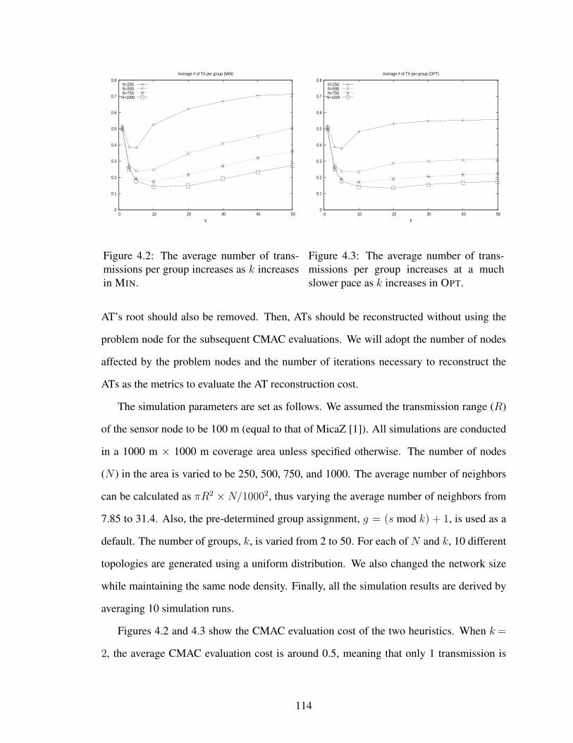
0
0.1
0.2
0.3
0.4
0.5
0.6
0.7
0.8
0 10 20 30 40 50
k
Average # of TX per group (MIN)
N=250 N=500 N=750
N=1000
Figure 4.2: The average number of trans-missions per group increases as k increasesin MIN.
0
0.1
0.2
0.3
0.4
0.5
0.6
0.7
0.8
0 10 20 30 40 50
k
Average # of TX per group (OPT)
N=250 N=500 N=750
N=1000
Figure 4.3: The average number of trans-missions per group increases at a muchslower pace as k increases in OPT.
AT’s root should also be removed. Then, ATs should be reconstructed without using the
problem node for the subsequent CMAC evaluations. We will adopt the number of nodes
affected by the problem nodes and the number of iterations necessary to reconstruct the
ATs as the metrics to evaluate the AT reconstruction cost.
The simulation parameters are set as follows. We assumed the transmission range (R)
of the sensor node to be 100 m (equal to that of MicaZ [1]). All simulations are conducted
in a 1000 m × 1000 m coverage area unless specified otherwise. The number of nodes
(N ) in the area is varied to be 250, 500, 750, and 1000. The average number of neighbors
can be calculated as πR2 × N/10002, thus varying the average number of neighbors from
7.85 to 31.4. Also, the pre-determined group assignment, g = (s mod k) + 1, is used as a
default. The number of groups, k, is varied from 2 to 50. For each of N and k, 10 different
topologies are generated using a uniform distribution. We also changed the network size
while maintaining the same node density. Finally, all the simulation results are derived by
averaging 10 simulation runs.
Figures 4.2 and 4.3 show the CMAC evaluation cost of the two heuristics. When k=
2, the average CMAC evaluation cost is around 0.5, meaning that only 1 transmission is
114
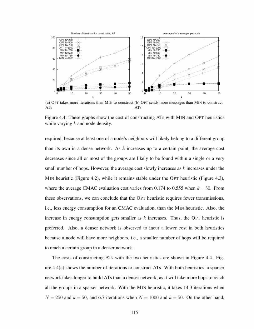
0
20
40
60
80
100
0 10 20 30 40 50
k
Number of iterations for constructing AT
OPT N=250 OPT N=500 OPT N=750
OPT N=1000MIN N=250 MIN N=500 MIN N=750
MIN N=1000
(a) OPT takes more iterations than MIN to constructATs
0
2
4
6
8
10
12
0 10 20 30 40 50
k
Average # of messages per node
OPT N=250 OPT N=500 OPT N=750
OPT N=1000MIN N=250 MIN N=500 MIN N=750
MIN N=1000
(b) OPT sends more messages than MIN to constructATs
Figure 4.4: These graphs show the cost of constructing ATs with MIN and OPT heuristicswhile varying k and node density.
required, because at least one of a node’s neighbors will likely belong to a different group
than its own in a dense network. As k increases up to a certain point, the average cost
decreases since all or most of the groups are likely to be found within a single or a very
small number of hops. However, the average cost slowly increases as k increases under the
MIN heuristic (Figure 4.2), while it remains stable under the OPT heuristic (Figure 4.3),
where the average CMAC evaluation cost varies from 0.174 to 0.555 when k= 50. From
these observations, we can conclude that the OPT heuristic requires fewer transmissions,
i.e., less energy consumption for an CMAC evaluation, than the MIN heuristic. Also, the
increase in energy consumption gets smaller as k increases. Thus, the OPT heuristic is
preferred. Also, a denser network is observed to incur a lower cost in both heuristics
because a node will have more neighbors, i.e., a smaller number of hops will be required
to reach a certain group in a denser network.
The costs of constructing ATs with the two heuristics are shown in Figure 4.4. Fig-
ure 4.4(a) shows the number of iterations to construct ATs. With both heuristics, a sparser
network takes longer to build ATs than a denser network, as it will take more hops to reach
all the groups in a sparser network. With the MIN heuristic, it takes 14.3 iterations when
N = 250 and k = 50, and 6.7 iterations when N = 1000 and k = 50. On the other hand,
115
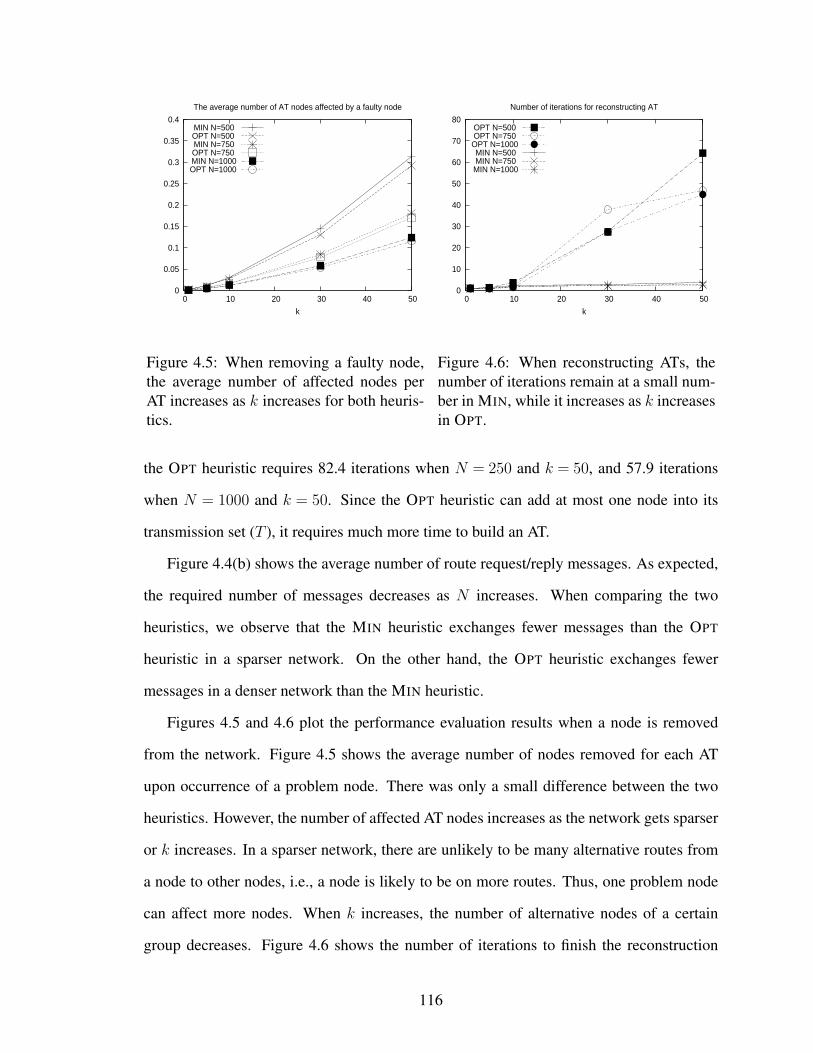
0
0.05
0.1
0.15
0.2
0.25
0.3
0.35
0.4
0 10 20 30 40 50
k
The average number of AT nodes affected by a faulty node
MIN N=500 OPT N=500 MIN N=750 OPT N=750 MIN N=1000OPT N=1000
Figure 4.5: When removing a faulty node,the average number of affected nodes perAT increases as k increases for both heuris-tics.
0
10
20
30
40
50
60
70
80
0 10 20 30 40 50
k
Number of iterations for reconstructing AT
OPT N=500 OPT N=750
OPT N=1000MIN N=500 MIN N=750
MIN N=1000
Figure 4.6: When reconstructing ATs, thenumber of iterations remain at a small num-ber in MIN, while it increases as k increasesin OPT.
the OPT heuristic requires 82.4 iterations when N = 250 and k = 50, and 57.9 iterations
when N = 1000 and k = 50. Since the OPT heuristic can add at most one node into its
transmission set (T ), it requires much more time to build an AT.
Figure 4.4(b) shows the average number of route request/reply messages. As expected,
the required number of messages decreases as N increases. When comparing the two
heuristics, we observe that the MIN heuristic exchanges fewer messages than the OPT
heuristic in a sparser network. On the other hand, the OPT heuristic exchanges fewer
messages in a denser network than the MIN heuristic.
Figures 4.5 and 4.6 plot the performance evaluation results when a node is removed
from the network. Figure 4.5 shows the average number of nodes removed for each AT
upon occurrence of a problem node. There was only a small difference between the two
heuristics. However, the number of affected AT nodes increases as the network gets sparser
or k increases. In a sparser network, there are unlikely to be many alternative routes from
a node to other nodes, i.e., a node is likely to be on more routes. Thus, one problem node
can affect more nodes. When k increases, the number of alternative nodes of a certain
group decreases. Figure 4.6 shows the number of iterations to finish the reconstruction
116

of ATs. MIN is found to take much fewer iterations than OPT. This means that it will
take much longer to construct ATs with the OPT heuristic when a node becomes faulty or
compromised.
We also evaluated the performance of ARCMA for different network sizes while main-
taining the same node density. However, it is found that the network size does not affect the
performance of ARCMA for the same node density, and thus, we did not repeat the result
here.
4.9 Conclusion
In this chapter, we proposed a novel security mechanism for DCS, called ARCMA, fo-
cusing on resilience against node-capture attacks. Under such attacks, securing DCS is very
difficult since attackers have accesses to all the valid keying materials extracted from the
compromised nodes. In ARCMA, sensor nodes collaboratively authenticate event-report,
event-query and query-response messages which typically travel multiple hops. Each sen-
sor node belongs to one of k groups, and builds and maintains an AT with k nodes, each
from a distinct group. With the help from the nodes in its AT, a sensor node can evaluate
CMACs to authenticate messages.
When an event is identified by a set of cooperating sensor nodes, they generate an event-
report with CMAC, which will then be forwarded to, and verified by, storage nodes. Before
a mobile user issues a query, he needs to collect k tokens by contacting k sensor nodes, one
from each distinct group. When a query is issued along with these tokens, it is authenticated
as was done for an event-report message, and then forwarded to storage nodes. Finally, the
storage node verifies and processes the valid message. Likewise, a response to the query
can be authenticated.
ARCMA is shown to be (k−1)-collusion resistant, i.e., the same level of security is
preserved as long as no more than (k− 1) nodes are captured. We also presented and
evaluated two heuristics (MIN and OPT) to build ATs. MIN builds ATs using the nearest
117

nodes from a specific group. This heuristic is constructed within fewer iterations both
when ATs are constructed from scratch and when ATs are reconstructed after revoking
faulty or compromised nodes. On the other hand, OPT incurs a lower operation cost (i.e.,
less transmissions to send one message to all the nodes in an AT) and a slower growth in the
operation cost, while it takes longer to build ATs, and the number of messages exchanged
to build an AT depends on the AT.
118

CHAPTER V
CONCLUSION
Wireless sensor networks (WSNs) are being deployed widely for physical-environment
monitoring. In a hybrid WSN, a large number of sensor nodes identify events of interest,
and a relatively small number of mobile nodes carried by humans or attached to vehicles
access sensor nodes to retrieve the information of identified events. Several network ser-
vices have been developed to support this application scenario, including localization, time
synchronization, and routing services.
This thesis proposes essential network services to better support WSN applications.
Currently available network services are inefficient or insecure when supporting applica-
tions in WSNs. Therefore, we design network services complementary to the existing
network services in the context of hybrid WSNs. The contributions of this thesis are sum-
marized as follows.
First, we propose a location service, called the distributed location service protocol
(DLSP), to provide sensor nodes with the location of mobile nodes to enable message de-
livery to mobile nodes using a geographic forward routing protocol. We provide systematic
methods to elect location servers among sensor nodes responsible for storing the location
information of mobile nodes, to publish location information of mobile nodes to those lo-
cation servers, and to process location queries for the mobile nodes’ location. We show
that the proposed protocol is more efficient than others, and reliable even in the presence
119

of holes.
Second, we present an algorithm, TRAVERSE, which identifies the boundaries of holes
in sensor networks. Holes are formed because of obstacles on the deployment area, node
failures, attacks, or some other events. Holes can degrade the performance of network ser-
vices on WSN. We also propose geographic forward routing with hole avoidance (GFRHA),
which utilizes the hole boundary information to detour packets around holes. We demon-
strate that GFRHA in conjunction with TRAVERSE significantly reduces the path length
under certain shapes of holes and the locations of sources and destinations.
Finally, we designed attack-resilient collaborative message authentication (ARCMA), a
mechanism for secure message delivery among sensor nodes or between a mobile node and
a sensor node. In ARCMA, sensor nodes collaboratively evaluate a collaborative message
authentication code (CMAC) to authenticate or verify messages. We provide key man-
agement mechanisms for ARCMA, and protocols to locate other sensor nodes which can
collaborate to authenticate a given message. ARCMA is designed to tolerate node-capture
attacks.
Future work can be pursued in the following directions.
• Performance improvement of DLSP: The performance of DLSP can be improved
by caching mobiles’ location at the sensor nodes, which forward location updates.
However, we need to restrict the number of mobiles’ locations cached in the sensor
nodes since their memory is very limited. We can study the effect of cache policies
on the performance of DLSP.
• Better hole summary for DHD: In GFRHA, an identified hole is summarized as a
circle, and messages are routed around the circle. However, a circle may not be a
tight bound for the given hole. Thus, with a tighter hole summary such as a convex
hull, GFRHA may achieve more performance gain. The trade-off between the perfor-
mance gain with tighter hole summaries and the cost for obtaining such summaries
may be studied.
120
• Secure location service and hole detection: Since an entire WSN can be subverted
by exploiting the weakest component, it is very important to secure each component
of the network. Thus, we can improve security of DLSP and TRAVERSE to improve
the security of the whole WSNs. ACRMA may be adopted to authenticate remote
messages of these protocols such as location-update and query messages in DLSP
and the hole summary information in DHD. In securing the protocols, node-capture
attacks will be considered as main threats, as they are in ARCMA.
121

BIBLIOGRAPHY
122
BIBLIOGRAPHY
[1] Crossbow MICAz datasheet. http://www.xbow.com/Products/Product pdf files/
Wireless pdf/MICAz Datasheet.pdf.
[2] The network simulator - ns-2. http://www.isi.edu/nsnam/ns/.
[3] TinyOS. http://www.tinyos.net.
[4] Proceedings of the Fifth Annual IEEE Communications Society Conference on Sensor,
Mesh and Ad Hoc Communications and Networks, SECON 2008, June 16-20, 2008,
Crowne Plaza, San Francisco International Airport, California, USA, 2008.
[5] E. Ayday, F. Delgosha, and F. Fekri. Location-aware security services for wireless
sensor networks using network coding. In Proceedings of the 26th IEEE International
Conference on Computer Communications (INFOCOM ’07), pages 1226–1234, May
2007.
[6] C. Blundo, A. D. Santis, A. Herzberg, S. Kutten, U. Vaccaro, and M. Yung. Perfectly-
secure key distribution for dynamic conferences. In CRYPTO ’92: Proceedings of the
12th Annual International Cryptology Conference on Advances in Cryptology, pages
471–486, 1993.
[7] P. Bose, P. Morin, I. Stojmenovic, and J. Urrutia. Routing with guaranteed delivery
in ad hoc wireless networks. Wirel. Netw., 7(6):609–616, 2001.
123
[8] N. Bulusu, J. Heidemann, D. Estrin, and T. Tran. Self-configuring localization sys-
tems: Design and experimental evaluation. Trans. on Embedded Computing Sys.,
3(1):24–60, 2004.
[9] T. Camp, J. Boleng, and V. Davies. A survey of mobility models for ad hoc network
research. Wireless Communication and Mobile Computing (WCMC): Special issue
on Mobile Ad Hoc Networking, 2002.
[10] Z. Chen, M. gyu Cho, and K. G. Shin. Design of location service for a hybrid network
of mobile actors and static sensors. In the 27th IEEE International Real-Time Systems
Symposium (RTSS ’06, pages 202–211, Dec. 2006.
[11] T. Dam and K. Langendoen. An adaptive energy-efficient mac protocol for wireless
sensor networks. In Proceedings of the 1st international conference on Embedded
netwroked sensor systems (SenSys ’03), 2003.
[12] S. M. Das, H. Pucha, and Y. C. Hu. Performance comparison of scalable location
services for geographic ad hoc routing. In Proceedings of the 24th Annual Joint
Conference of the IEEE Computer and Communications Societies (INFOCOM ’05),
pages 217–228, 2005.
[13] W. Du, J. Deng, Y. Han, S. Chen, and P. Varshney. A key management scheme
for wireless sensor networks using deployment knowledge. In Proceedings of the
23rd Annual Joint Conference of the IEEE Computer and Communications Societies
(INFOCOM ’04), volume 1, pages –597, 2004.
[14] W. Du, J. Deng, Y. S. Han, and P. K. Varshney. A pairwise key pre-distribution
scheme for wireless sensor networks. In Proceedings of the 10th ACM conference on
Computer and communications security (CCS ’03), pages 42–51, 2003.
[15] A. El-Hoiydi and J. Decotignie. WiseMAC, an ultra low power mac protocol for the
124
WiseNET wireless sensor network. In IEEE International Symposium on Computers
and Communications, 2004.
[16] J. Elson, L. Girod, and D. Estrin. Fine-grained network time synchronization using
reference broadcasts. SIGOPS Oper. Syst. Rev., 36(SI):147–163, 2002.
[17] L. Eschenauer and V. D. Gligor. A key-management scheme for distributed sensor
networks. In Proceedings of the 9th ACM conference on Computer and communica-
tions security (CCS ’03), pages 41–47, 2002.
[18] Q. Fang, J. Gao, and L. Guibas. Locating and bypassing routing holes in sensor
networks. In INFOCOM 2004. Twenty-third AnnualJoint Conference of the IEEE
Computer and Communications Societies, volume 4, pages 2458–2468vol.4, 7-11
March 2004.
[19] R. Flury and R. Wattenhofer. MLS: an efficient location service for mobile ad hoc
networks. In Proceedings of the 7th ACM international symposium on Mobile ad hoc
networking and computing (MobiHoc ’06), pages 226–237, 2006.
[20] R. Fonseca, S. Ratnasamy, J. Zhao, C. Ee, D. Culler, S. Shenker, and I. Stoica. Beacon
vector routing: Scalable point-to-point routing in wireless sensornets. In Proceedings
of NSDI 2005, pages 329–342, 2005.
[21] S. Funke. Topological hole detection in wireless sensor networks and its applications.
In DIALM-POMC ’05: Proceedings of the 2005 joint workshop on Foundations of
mobile computing, pages 44–53, 2005.
[22] S. Ganeriwal, R. Kumar, and M. B. Srivastava. Timing-sync protocol for sensor net-
works. In Proceedings of the 1st international conference on Embedded netwroked
sensor systems (SenSys ’03), pages 138–149, 2003.
125
[23] S. Ganeriwal and M. B. Srivastava. Reputation-based framework for high integrity
sensor networks. In Proceedings of the 2nd ACM workshop on Security of ad hoc and
sensor networks (SASN ’04), pages 66–77, 2004.
[24] D. Ganesan, D. Estrin, and J. Heidemann. Dimensions: why do we need a new
data handling architecture for sensor networks? SIGCOMM Comput. Commun. Rev.,
33(1):143–148, 2003.
[25] A. Ghose, J. Grossklags, and J. Chuang. Resilient data-centric storage in wireless ad-
hoc sensor networks. In MDM ’03: Proceedings of the 4th International Conference
on Mobile Data Management, pages 45–62, 2003.
[26] T. Goff, N. B. Abu-Ghazaleh, D. S. Phatak, and R. Kahvecioglu. Preemptive routing
in ad hoc networks. In Mobile Computing and Networking, pages 43–52, 2001.
[27] B. Greenstein, D. Estrin, R. Govindan, S. Ratnasamy, and S. Shenker. DIFS: a dis-
tributed index for features in sensor networks. In Sensor Network Protocols and Ap-
plications, 2003. Proceedings of the First IEEE. 2003 IEEE International Workshop
on, pages 163–173, 2003.
[28] M. Grossglauser and M. Vetterli. Locating nodes with ease: last encounter routing in
ad hoc networks through mobility diffusion. In Proceedings of the 22nd Annual Joint
Conference of the IEEE Computer and Communications Societies (INFOCOM’03),
volume 3, pages 1954–1964 vol.3, March-3 April 2003.
[29] R. B. Hayward, J. P. Spinrad, and R. Sritharan. Improved algorithms for weakly
chordal graphs. ACM Trans. Algorithms, 3(2):14, 2007.
[30] T. He, C. Huang, B. M. Blum, J. A. Stankovic, and T. Abdelzaher. Range-free lo-
calization schemes for large scale sensor networks. In Proceedings of the 9th annual
international conference on Mobile computing and networking (MobiCom ’03), pages
81–95, 2003.
126
[31] L. Hu and D. Evans. Localization for mobile sensor networks. In Proceedings of the
10th annual international conference on Mobile computing and networking (Mobi-
Com ’04), pages 45–57, 2004.
[32] Q. Huang, J. Cukier, H. Kobayashi, B. Liu, and J. Zhang. Fast authenticated key es-
tablishment protocols for self-organizing sensor networks. In Proceedings of the 2nd
ACM international workshop on Wireless sensor networks and applications (WSNA
’03), pages 141–150, 2003.
[33] B. Karp and H. T. Kung. GPSR: greedy perimeter stateless routing for wireless net-
works. In Proceedings of the 6th annual international conference on Mobile comput-
ing and networking (MobiCom ’00), pages 243–254, 2000.
[34] W. Kieß, H. Fußler, J. Widmer, and M. Mauve. Hierarchical location service for
mobile ad-hoc networks. SIGMOBILE Mob. Comput. Commun. Rev., 8(4):47–58,
2004.
[35] H. Kim and J. C. Hou. Improving protocol capacity with model-based frame schedul-
ing in ieee 802.11-operated wlans. In Proceedings of the 9th annual international
conference on Mobile computing and networking (MobiCom ’03), pages 190–204,
2003.
[36] S. Kumar, T. H. Lai, and J. Balogh. On k-coverage in a mostly sleeping sensor net-
work. In Proceedings of the 10th annual international conference on Mobile comput-
ing and networking (MobiCom ’04), pages 144–158, 2004.
[37] S. M. LaValle. Planning Algorithms. Cambridge University Press, Cambridge, U.K.,
2006. Available at http://planning.cs.uiuc.edu/.
[38] L. Lazos and R. Poovendran. SeRLoc: secure range-independent localization for
wireless sensor networks. In Proceedings of the 2004 ACM workshop on Wireless
security (WiSe ’04), pages 21–30, 2004.
127
[39] S. Lee, B. Bhattacharjee, and S. Banerjee. Efficient geographic routing in multihop
wireless networks. In Proceedings of the 6th ACM international symposium on Mo-
bile ad hoc networking and computing (MobiHoc ’05), pages 230–241, 2005.
[40] J. Li, J. Jannotti, D. S. J. D. Couto, D. R. Karger, and R. Morris. A scalable location
service for geographic ad hoc routing. In Proceedings of the 6th annual international
conference on Mobile computing and networking (MobiCom ’00), pages 120–130,
2000.
[41] M. Li and Y. Liu. Rendered path: range-free localization in anisotropic sensor net-
works with holes. In Proceedings of the 13th annual international conference on
Mobile computing and networking (MobiCom ’07), pages 51–62, 2007.
[42] X. Li, Y. J. Kim, R. Govindan, and W. Hong. Multi-dimensional range queries in
sensor networks. In Proceedings of the 1st international conference on Embedded
netwroked sensor systems (SenSys ’03), pages 63–75, 2003.
[43] Y. Li, W. Ye, and J. Heidemann. Energy and latency control in low duty cycle MAC
protocols. In Proceedings of the IEEE Wireless Communications and Networking
Conference, March 2005.
[44] D. Liu and P. Ning. Establishing pairwise keys in distributed sensor networks. In
Proceedings of the 10th ACM conference on Computer and communications security
(CCS ’03), pages 52–61, 2003.
[45] A. Mainwaring, J. Polastre, R. Szewczyk, D. Culler, and J. Anderson. Wireless sen-
sor networks for habitat monitoring. In Proceedings of the 1st ACM international
workshop on Wireless sensor networks and applications (WSNA ’02), 2002.
[46] D. Malan, M. Welsh, and M. Smith. A public-key infrastructure for key distribution
in TinyOS based on elliptic curve cryptography. In Proceedings of the 1st Annual
128
IEEE Communications Society Conference on Sensor and Ad Hoc Communications
and Networks (SECON ’04), pages 71–80, 2004.
[47] M. Maroti, P. Volgyesi, S. Dora, B. Kusy, A. Nadas, A. Ledeczi, G. Balogh, and
K. Molnar. Radio interferometric geolocation. In SenSys ’05: Proceedings of the 3rd
international conference on Embedded networked sensor systems, pages 1–12, 2005.
[48] D. Moore, J. Leonard, D. Rus, and S. Teller. Robust distributed network localization
with noisy range measurements. In SenSys ’04: Proceedings of the 2nd international
conference on Embedded networked sensor systems, pages 50–61, 2004.
[49] T. Muetze, P. Stuedi, F. Kuhn, and G. Alonso. Understanding radio irregularity in
wireless networks. In SECON [4], pages 82–90.
[50] S. D. Nikolopoulos and L. Palios. Hole and antihole detection in graphs. In SODA
’04: Proceedings of the fifteenth annual ACM-SIAM symposium on Discrete algo-
rithms, pages 850–859, 2004.
[51] S. Olariu, M. Eltoweissy, and M. Younis. ANSWER: autonomous wireless sensor
network. In Proceedings of the 1st ACM international workshop on Quality of service
& security in wireless and mobile networks (Q2SWinet ’05), 2005.
[52] J. Ortiz, C. R. Baker, D. Moon, R. Fonseca, and I. Stoica. Beacon location service:
a location service for point-to-point routing in wireless sensor networks. In Pro-
ceedings of the 4th International Symposium on Information Processing in Sensor
Networks (IPSN 2007), pages 166–175, 2007.
[53] B. Parno, M. Luk, E. Gaustad, and A. Perrig. Secure sensor network routing: A
clean-slate approach. In CoNEXT’06: Proceedings of the 2006 ACM conference on
Emerging network experiment and technology, 2006.
129

[54] J. Polastre, J. Hill, and D. Culler. Versatile low power media access for wireless
sensor networks. In Proceedings of the 2nd international conference on Embedded
netwroked sensor systems (SenSys ’04), 2004.
[55] B. Przydatek, D. Song, and A. Perrig. SIA: secure information aggregation in sensor
networks. In Proceedings of the 1st international conference on Embedded netwroked
sensor systems (SenSys ’03), pages 255–265, 2003.
[56] S. Ratnasamy, B. Karp, L. Yin, F. Yu, D. Estrin, R. Govindan, and S. Shenker. GHT:
a geographic hash table for data-centric storage. In Proceedings of the 1st ACM inter-
national workshop on Wireless sensor networks and applications (WSNA ’02), pages
78–87, 2002.
[57] K. Ren, W. Lou, and Y. Zhang. Leds: Providing location-aware end-to-end data
security in wireless sensor networks. In Proceedings of the 25th IEEE International
Conference on Computer Communications (INFOCOM ’06), pages 1–12, April 2006.
[58] N. Sadagopan, F. Bai, B. Krishnamachari, and A. Helmy. PATHS: analysis of PATH
duration statistics and their impact on reactive manet routing protocols. In Proceed-
ings of the 4th ACM international symposium on Mobile ad hoc networking and com-
puting (MobiHoc ’03), pages 245–256, 2003.
[59] A. Savvides, C.-C. Han, and M. B. Strivastava. Dynamic fine-grained localization in
ad-hoc networks of sensors. In Proceedings of the 7th annual international confer-
ence on Mobile computing and networking (MobiCom ’01), pages 166–179, 2001.
[60] M. Shao, S. Zhu, W. Zhang, and G. Cao. pdcs: Security and privacy support for data-
centric sensor networks. In INFOCOM 2007. 26th IEEE International Conference on
Computer Communications. IEEE, pages 1298–1306, May 2007.
[61] S. Singh and C. S. Raghavendra. PAMAS – power aware multi-access protocol with
130

signalling for ad hoc networks. SIGCOMM Comput. Commun. Rev., 28(3):5–26,
1998.
[62] I. Stojmenovic. A routing strategy and quorum based location update scheme for ad
hoc wireless networks. Technical report, University of Ottawa, 1999.
[63] W. Su and I. F. Akyildiz. Time-diffusion synchronization protocol for wireless sensor
networks. IEEE/ACM Trans. Netw., 13(2):384–397, 2005.
[64] K. Sun, P. Ning, and C. Wang. TinySeRSync: secure and resilient time synchro-
nization in wireless sensor networks. In Proceedings of the 13th ACM conference on
Computer and communications security (CCS ’06), pages 264–277, 2006.
[65] P. F. Tsuchiya. The landmark hierarchy: A new hierarchy for routing in very large
networks. In Proceedings of SIGCOMM’88, Aug. 1988.
[66] A. C. Viana, M. D. de Amorim, S. Fdida, Y. Viniotis, and J. F. de Rezende. Easily-
managed and topology-independent location service for self-organizing networks. In
Proceedings of the 6th ACM international symposium on Mobile ad hoc networking
and computing (MobiHoc ’05), pages 193–204, 2005.
[67] D. Wagner. Resilient aggregation in sensor networks. In Proceedings of the 2nd ACM
workshop on Security of ad hoc and sensor networks (SASN ’04), pages 78–87, 2004.
[68] R. Watro, D. Kong, S. fen Cuti, C. Gardiner, C. Lynn, and P. Kruus. TinyPK: se-
curing sensor networks with public key technology. In Proceedings of the 2nd ACM
workshop on Security of ad hoc and sensor networks (SASN ’04), pages 59–64, 2004.
[69] C. Westpha. Little tom thumb went straight home: Asymptotic behavior of a rout-
ing protocol in ad-hoc networks with a mobile access point. In Proceedings of the
26th IEEE International Conference on Computer Communications (INFOCOM ’07),
pages 1847–1856, May 2007.
131

[70] Y. Xue, B. Li, and K. Nahrstedt. A scalable location management scheme in mobile
ad-hoc networks. In Proceedings of IEEE Conference on Local Computer Networks,
pages 102–111, Nov 2001.
[71] H. Yang, F. Ye, Y. Yuan, S. Lu, and W. Arbaugh. Toward resilient security in wireless
sensor networks. In Proceedings of the 6th ACM international symposium on Mobile
ad hoc networking and computing (MobiHoc ’05), pages 34–45, 2005.
[72] F. Ye, H. Luo, J. Cheng, S. Lu, and L. Zhang. A two-tier data dissemination model for
large-scale wireless sensor networks. In Proceedings of the 8th annual international
conference on Mobile computing and networking (MobiCom ’02), pages 148–159,
2002.
[73] F. Ye, H. Luo, S. Lu, and L. Zhang. Statistical en-route filtering of injected false
data in sensor networks. In Proceedings of the 23rd Annual Joint Conference of the
IEEE Computer and Communications Societies (INFOCOM ’04), volume 4, pages
2446–2457 vol.4, 2004.
[74] F. Ye, H. Luo, S. Lu, and L. Zhang. Statistical en-route filtering of injected false data
in sensor networks. IEEE Journal on Selected Areas in Communications, 23(4):839–
850, 2005.
[75] W. Ye and J. Heidemann. Ultra-low duty cycle mac with scheduled channel polling.
Technical Report ISI-TR-2005-604b, USC/Information Sciences Institute, July 2005.
[76] W. Ye, J. Heidemann, and D. Estrin. An energy-efficient mac protocol for wireless
sensor networks. In Proceedings of the 21st Annual Joint Conference of the IEEE
Computer and Communications Societies (INFOCOM’02), volume 3, pages 1567–
1576, 23-27 June 2002.
[77] J. Yick, B. Mukherjee, and D. Ghosal. Wireless sensor network survey. Computer
Networks, 52(12):2292–2330, Aug. 2008.
132
[78] J. Yoon, M. Liu, and B. Noble. Sound mobility models. In Proceedings of the 9th an-
nual international conference on Mobile computing and networking (MobiCom ’03),
Sept. 2003.
[79] W. Zhang, H. Song, S. Zhu, and G. Cao. Least privilege and privilege deprivation:
towards tolerating mobile sink compromises in wireless sensor networks. In Pro-
ceedings of the 6th ACM international symposium on Mobile ad hoc networking and
computing (MobiHoc ’05), pages 378–389, 2005.
[80] Y. Zhang, W. Liu, W. Lou, and Y. Fang. Location-based compromise-tolerant secu-
rity mechanisms for wireless sensor networks. IEEE Journal on Selected Areas in
Communications, 24(2):247–260, Feb. 2006.
[81] Q. Zheng, X. Hong, and S. Ray. Recent advances in mobility modeling for mobile
ad hoc network research. In ACM-SE 42: Proceedings of the 42nd annual Southeast
regional conference, pages 70–75, 2004.
[82] G. Zhou, T. He, S. Krishnamurthy, and J. A. Stankovic. Impact of radio irregularity
on wireless sensor networks. In MobiSys ’04: Proceedings of the 2nd international
conference on Mobile systems, applications, and services, pages 125–138, 2004.
[83] S. Zhu, S. Setia, S. Jajodia, and P. Ning. An interleaved hop-by-hop authentication
scheme for filtering of injected false data in sensor networks. In Proceedings of the
2004 Symposium on Security and Privacy, pages 259–271, 2004.
133