Efficiency in Auctions with Private and Common Values:

An Experimental Study

Jacob K. Goeree and Theo Offerman*

May 2000

ABSTRACT

Auctions generally do not lead to efficient outcomes when the expected value of theobject for sale depends on both private and common value information. We report a series offirst-price auction experiments to test three key predictions of auctions with private andcommon values: (i) inefficiencies grow with the uncertainty about the common value whilerevenues fall, (ii) increased competition results in more efficient outcomes and higherrevenues, and (iii) revenues and efficiency are higher when information about the commonvalue is publicly released. We compare the predictions of several bidding models, includingNash, when examining these issues. A model in which a fraction of the bidders falls prey toa winner’s curse and decision-making is noisy, best describes bidding behavior. We find thatrevenues and efficiency are positively affected by increased competition and a reduction inuncertainty about the common value. The public release of high-quality information aboutthe common value also has positive effects on efficiency, although less so than predicted byNash equilibrium bidding.

JEL Classification: C72, D44.Keywords: Auctions, experiments, winner’s curse, efficiency, information disclosure,competition.

* Goeree: Department of Economics, 114 Rouss Hall, University of Virginia, P.O. Box 400182, CharlottesvilleVA 22904-4182; Offerman: CREED, University of Amsterdam, Roetersstraat 11, 1018 WB Amsterdam, TheNetherlands. We acknowledge financial support from the Bankard Fund at the University of Virginia and from theDutch Organization for Scientific Research (NWO). We would like to thank Charlie Holt, Deniz Selman, andparticipants at the Public Choice Society Meetings (2000) for useful suggestions.

1

1. Introduction

Auctions are typically classified as either "private value" or "common value." In

private value auctions, bidders know their own value for the commodity for sure but are

unaware of others’ valuations (e.g. the sale of a painting). In contrast, in common value

auctions, each bidder receives a noisy signal about the commodity’s value, which is the same

for all (e.g. firms competing for the rights to drill for oil). While this dichotomy is

convenient from a theoretical point of view, most real-world auctions exhibit both private and

common value elements. In the recent spectrum auctions conducted by the FCC, for example,

the different cost structures of the bidding firms constituted a private value element, while the

uncertain demand for the final consumer product added a common value part. Alternatively,

in takeover battles, bidders’ valuations are determined by private synergistic gains in addition

to the target’s common market value.1

By focusing on the "extreme" cases, the literature has inadvertently spread the belief

that auctions generally lead to efficient allocations. In (symmetric) private value auctions,

optimal bids are increasing in bidders’ values so the object is awarded to whom it is worth

the most, and in common value auctions, any allocation is trivially efficient. When both

private and common value elements play a role, however, inefficiencies should be expected.

The simple intuition for this result is that a bidder with an inferior private value but an overly

optimistic conjecture about the common value may outbid a rival with a superior private

value. The possibility of inefficiencies in multi-signal auctions was first discussed by Maskin

(1992) and further explored by Dasgupta and Maskin (1999), Jehiel and Moldovanu (1999),

Pesendorfer and Swinkels (1999), and Goeree and Offerman (1999).

This paper reports a series of first-price auction experiments in which bidders receive

a private and a common value signal.2 To determine the optimal bid, the two pieces of

1 Even the standard examples of purely private or purely common value auctions are not convincing. When apainting is auctioned, for instance, it may be resold in the future and the resale price will be the same for all bidders,which adds a common value element. And in the oil drilling example, a firm’s cost of exploiting the tract adds aprivate value element.

2 Kirchkamp and Moldovanu (2000) report an experiment that compares the efficiency properties of the English

auction and the second-price auction when bidders’ valuations are interdependent.

2

information have to be combined and the relative weights bidders assign to each signal

determines the efficiency of the resulting allocation. For instance, if bidders completely

ignore their common value signal, the auction turns into a fully efficient private value auction.

In contrast, when bidders ignore their private value information, the auction is no more

efficient than a random allocation rule. Rational bidders react to both pieces of information,

resulting in some intermediate degree of inefficiency. One goal of this paper is to measure

the extent of inefficiencies that result with financially motivated human bidders.

Observed bids will differ from rational ones when subjects do not (sufficiently)

incorporate the negative information conveyed by winning into their bids. Indeed, there exists

substantial experimental and empirical evidence that in purely common value auctions,

bidders often ignore this adverse selection effect and forgo some profits as a result: the

winner’s curse.3 In auctions with both private and common values such naive bidders may

cause inefficiencies when they put too much weight on their own common value signal. To

separate efficiency from winner’s curse issues, the common value in our experiment is the

average of bidders’ signals. This design allows bidders to fall prey to a winner’s curse, by

replacing others’ common value signals by their unconditional expected value, without

affecting efficiency. As long as bidders assign the same weight to their own common value

signal as rational bidders would, efficiency remains unchanged. Of course, the amount paid

by a naive winner will be higher (and may even exceed the object’s value), but this monetary

transfer from the winning bidder to the seller does not affect efficiency.

A second goal of this paper is to systematically explore factors that affect efficiency

and to test the effectiveness of policies aimed at reducing inefficiencies. For example, when

licenses to operate in a market are auctioned, interested firms will have to estimate the

uncertain (but common) demand for the consumer product they will sell. There will be more

uncertainty associated with licenses for new markets (e.g. wireless local loop frequencies for

3 For experimental evidence, see Bazerman and Samuelson (1983), Kagel and Levin (1986), Dyer, Kagel, andLevin (1989), Kagel, Levin, Battalio, and Meyer (1989), Lind and Plott (1991), Garvin and Kagel (1994), Levin,Kagel, and Richard (1996), Avery and Kagel (1997), Cox, Dinkin, and Smith (1998), and Kagel and Levin (1999).Field studies also suggest that bidders are bothered by a winner’s curse, see e.g. Capen, Clapp, and Campbell (1971),Roll (1986), Thaler (1988), and Ashenfelter and Genesove (1992).

3

multi-media applications) than with licenses for well-established markets (e.g. vendor

locations at fairs). Intuitively, an increase in uncertainty about the common value makes the

private values less important and causes efficiency to fall. In addition, with more uncertainty

about the common value, bids have to be more cautious to avoid a winner’s curse, resulting

in higher profits for the bidders and less revenue for the seller.

Another important determinant for efficiency of market outcomes is (perfect)

competition (e.g. Stigler, 1987). In purely common value auctions, perfect competition also

leads to "information aggregation," i.e. the winning bid converges to the actual value of the

commodity for sale (Wilson, 1977). In auctions with private and common values, perfect

competition leads to both information aggregation and full efficiency. These positive effects

of competition are not limited to the case of an infinite number of bidders, however: even a

moderate increase in the number of bidders (e.g. from three to six) is predicted to have a

substantial effect on efficiency and revenues. The reason for this "small numbers" effect is

that bidders weigh their common value information substantially less even if there is only a

moderate increase in competition. Hence, the private value differences become more

important and an efficient outcome more likely. In fact, the introduction of new bidders

makes the auction more efficient even when these bidders themselves have no chance of

winning (see Goeree and Offerman, 1999).

Finally, the seller often possesses information about the object for sale and the public

disclosure of such information affects bidding behavior. Milgrom and Weber (1982) have

shown that the public release of information is in the auctioneer’s best interest because it

raises revenues. Elsewhere we have shown that public information release also raises

efficiency. The resulting increase in total surplus generated by the auction benefits the seller,

not the winning bidder, and the predicted effects on efficiency and revenues are stronger the

higher the quality of the public information (Goeree and Offerman, 1999).

This paper investigates the empirical validity of these theoretical predictions, i.e. the

effects of uncertainty about the common value, competition, and information disclosure on

efficiency and revenues. The order of topics is as follows: the design of the auctions is

explained in section 2. The Nash bidding functions and other theoretical benchmark models

are derived in section 3, together with some comparative statics results. In section 4 we

4

investigate the effects of the winner’s curse in auctions with private and common values. In

sections 5 and 6 we focus on how bidders process the private and common value signal, and

report the realized level of efficiency. The effects of uncertainty about the common value,

the public release of information, and increased competition are dealt with in section 7.

Section 8 concludes. The Appendices contain instructions, the Nash equilibrium bids for one

of the treatments, and figures that show actual and predicted bids in each treatment.

2. Design of the Auctions

Bidder i’s valuation for the object for sale consists of a private value, ti, and the

common value, V. The realization of V is unknown at the time of bidding, but is revealed

after the bidding phase. When bidder i wins the auction with a bid bi, she receives a net

amount of V + ti - bi, where the common value is the average of bidders’ signals:

This formulation for the common value has previously been used in both theoretical and

(1)

experimental work.4 An advantage of (1) is that it is easier to explain and understand than

the "traditional" formulation of the common value, where V has some known prior distribu-

tion and bidders’ signals are draws conditional on the particular realization of V (Wilson,

1970). While being simpler, (1) captures the two main features of the traditional formulation:

(i) the value of the object for sale is the same for all bidders, and (ii) in order not to fall prey

to a winner’s curse, bidders should take into account the information conveyed in winning.

Holt and Sherman (2000), for instance, report clear evidence of a winner’s curse in a two-

person first-price auction experiment using the formulation in (1), and Avery and Kagel

(1997) find similar evidence in a second-price auction.

The (completely computerized) experiment consisted of two parts; subjects received

the instructions for part 2 only after all twenty periods of part 1 were finished (see Appendix

4 Theoretical papers using this formulation include Bikchandani and Riley (1991), Albers and Harstad (1991),Krishna and Morgan (1997), Klemperer (1998), Bulow and Klemperer (1999) and Bulow, Huang and Klemperer(1999).

5

A for a translation of the instructions).5 In the experiment, subjects earned points, which

were exchanged into guilders at the end of the experiment at a rate of 4 points = 1 guilder (≈

$0.50). In total we conducted seven treatments: low-3, high-3, high-6, low-3+, high-3+, high-

6+, high-3++. The labels "low" and "high" indicate whether the variance of the common

value distribution was small or large, the number indicates group size, and the "+" (or "++")

sign indicates that subjects were once (twice) experienced. For statistical reasons, group-

composition was kept constant during the whole experiment, although subjects did not know

this, to avoid repeated-game effects.

Part 1. The Basic Setup

The first part of the experiment lasted for 20 periods. Bidders were given a starting

capital of 120 points, which they did not have to pay back. In each period, subjects’ private

values, ti, were uniformly distributed between 75 and 125, i.e. ti ∼ U[75,125]. Common value

signals were U[0,200] distributed in the high-3 and high-6 treatments, and were U[75,125]

distributed in the low-3 treatments. Both private and common value signals were i.i.d. across

subjects and periods, and the procedure for generating the signals was common knowledge.

Bids were restricted to lie between the lowest and highest possible valuation for the

commodity: in treatments low-3 and low-3+, subjects had to enter integer bids between 150

and 250 points, while in the other treatments bids had to be between 75 and 325 points. At

the end of a period subjects were told the bids in their group (ordered from high to low), the

common value, and whether or not they won the auction.6 They only received information

about others’ bids, not about others’ private or common value signals. Finally, the winner’s

profit was communicated only to the winner.

Part 2. Public Information Disclosure

The second part lasted from periods 21 to 30, and was designed to evaluate the effects

of public information release on efficiency, revenues, and profits. While the effects of

5 The experiment was programmed using the Rat-Image Toolbox, see Abbink and Sadrieh (1995).

6 In case of a tie, the winner was selected at random from the highest bidders.

6

increased competition and increased uncertainty about the common value were investigated

using a between subject design, we used a within subject design to determine the effects of

public information release. In each period, subjects made two decisions, the first decision

similar to that of part 1. After all subjects made their first decision, they received an

additional signal about the value of the object for sale, the auctioneer’s signal, and were

asked to bid again.7 The auctioneer’s signal was an independent draw from the same

distribution as the common value signals of the bidders. Everyone in the group received the

same auctioneer’s signal, and subjects’ private and common value signals for the second

decision were the same as for the first. The common value in part 2 was:

where v0 represents the auctioneer’s signal.

(2)

The implicit assumption underlying (2) is that the auctioneer’s signal has the same

precision as that of the bidders. One way to model a more precise auctioneer’s signal is to

give it more weight than the bidders’ signals.8 This was the case in treatment high-3++, for

which the common value in part 2 was calculated as:

Decisions with and without an auctioneer signal had an equal chance of being selected

(3)

for payment, and subjects learned which decision was chosen only after everyone had made

both decisions.9 They only received information pertaining to the decision that was selected,

and the information provided was analogous to that in part 1.

7 This procedure to evaluate the effects of an auctioneer report does not affect subjects’ choices in an undesiredway (Kagel and Levin, 1986, and Kagel, Harstad, and Levin, 1987).

8 This can be motivated as follows: suppose the variance of the bidders’ signals is σ2b (the same for all bidders)

and the variance of the auctioneer’s signal is σ2a. The "best" (i.e. unbiased and smallest variance) estimator of the

commodity’s value is then given by V = (λ v0 + Σni=1 vi)/(n+λ) where λ = σ2

b/σ2a is a measure of the (relative) quality

of the auctioneer’s information. The formulation in (2) corresponds to λ = 1 or σ2a = σ2

b, and (3) corresponds to λ =7 or σ2

a = σ2b/7.

9 A subject’s starting capital in period 21 equaled the total amount earned in part 1 plus a 60-point bonus.

7

Subjects and Bankruptcy

We conducted sessions with both inexperienced and experienced subjects, who were

recruited at the University of Amsterdam. The experiment was finished within two hours and

subjects made 61.25 guilders (≈ $30.60) on average. Their starting capital of 120 points

provided some buffer against bankruptcy.10 A subject went bankrupt when her cash balance

became negative, in which case she was asked to leave the experiment without receiving any

money. If a subject went bankrupt in a treatment with 6 bidders per group, the computer bid

0 for this subject for the remainder of the experiment. The other bidders in the group then

proceeded as before, now with one less opponent.11 If a subject went bankrupt in a

treatment with 3 bidders per group, the computer submitted Nash bids for this person for the

remainder of the experiment. (We did not use 0 bids in this case because we feared it would

make collusion too easy.) The other two bidders proceeded as before, now facing one

"human" and one "computerized Nash" opponent. The periods after a bankruptcy in a group

of three were played out only to give the remaining two bidders a chance to make some

money: the data from these periods are discarded.

Subjects who did not go bankrupt could voluntarily subscribe for one of the experi-

enced sessions. (Subjects who went bankrupt were not given this opportunity.) The majority

of subjects in experienced sessions participated in the same treatment as in their inexperienced

session. Treatment high-3++ was conducted two months after the other treatments, and

subjects in this treatment had participated in two earlier sessions. Table 1 summarizes the

different treatments and the number of participants.

3. Theoretical Background

While few people would dispute that most real-world auctions exhibit both private and

common value features, surprisingly little is known about their equilibrium properties. The

difficulty with multiple signals is how to combine the different pieces of information into a

10 Even when everyone plays according to the Nash strategy, there is some chance that the winner loses money.

11 Of course, if one of six bidders enters a zero bid, the theoretical predictions are affected (Nash andalternative models). We take this into account when analyzing the data.

8

single statistic that can be mapped into a bid (Milgrom and Weber, 1982, p.1097). This is

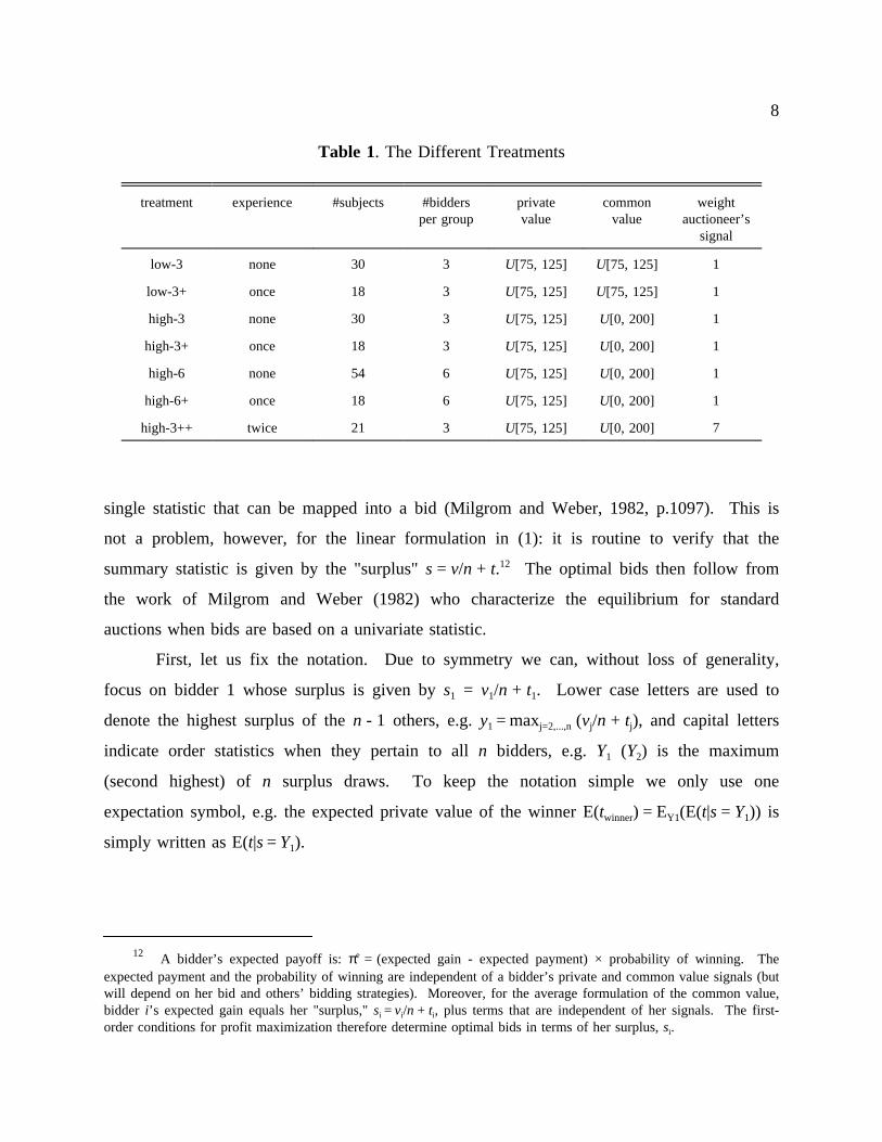
Table 1. The Different Treatments

treatment experience #subjects #biddersper group

privatevalue

commonvalue

weightauctioneer’s

signal

low-3 none 30 3 U[75, 125] U[75, 125] 1

low-3+ once 18 3 U[75, 125] U[75, 125] 1

high-3 none 30 3 U[75, 125] U[0, 200] 1

high-3+ once 18 3 U[75, 125] U[0, 200] 1

high-6 none 54 6 U[75, 125] U[0, 200] 1

high-6+ once 18 6 U[75, 125] U[0, 200] 1

high-3++ twice 21 3 U[75, 125] U[0, 200] 7

not a problem, however, for the linear formulation in (1): it is routine to verify that the

summary statistic is given by the "surplus" s = v/n + t.12 The optimal bids then follow from

the work of Milgrom and Weber (1982) who characterize the equilibrium for standard

auctions when bids are based on a univariate statistic.

First, let us fix the notation. Due to symmetry we can, without loss of generality,

focus on bidder 1 whose surplus is given by s1 = v1/n + t1. Lower case letters are used to

denote the highest surplus of the n - 1 others, e.g. y1 = maxj=2,...,n (vj/n + tj), and capital letters

indicate order statistics when they pertain to all n bidders, e.g. Y1 (Y2) is the maximum

(second highest) of n surplus draws. To keep the notation simple we only use one

expectation symbol, e.g. the expected private value of the winner E(twinner) = EY1(E(t|s = Y1)) is

simply written as E(t|s = Y1).

12 A bidder’s expected payoff is: πe = (expected gain - expected payment) × probability of winning. Theexpected payment and the probability of winning are independent of a bidder’s private and common value signals (butwill depend on her bid and others’ bidding strategies). Moreover, for the average formulation of the common value,bidder i’s expected gain equals her "surplus," si = vi/n + ti, plus terms that are independent of her signals. The first-order conditions for profit maximization therefore determine optimal bids in terms of her surplus, si.

9

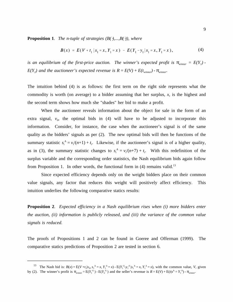
Proposition 1. The n-tuple of strategies (B( ),...,B( )), where

is an equilibrium of the first-price auction. The winner’s expected profit is πwinner = E(Y1) -

(4)

E(Y2) and the auctioneer’s expected revenue is R = E(V) + E(twinner) - πwinner.

The intuition behind (4) is as follows: the first term on the right side represents what the

commodity is worth (on average) to a bidder assuming that her surplus, x, is the highest and

the second term shows how much she "shades" her bid to make a profit.

When the auctioneer reveals information about the object for sale in the form of an

extra signal, v0, the optimal bids in (4) will have to be adjusted to incorporate this

information. Consider, for instance, the case when the auctioneer’s signal is of the same

quality as the bidders’ signals as per (2). The new optimal bids will then be functions of the

summary statistic siA = vi/(n+1) + ti. Likewise, if the auctioneer’s signal is of a higher quality,

as in (3), the summary statistic changes to siA = vi/(n+7) + ti. With this redefinition of the

surplus variable and the corresponding order statistics, the Nash equilibrium bids again follow

from Proposition 1. In other words, the functional form in (4) remains valid.13

Since expected efficiency depends only on the weight bidders place on their common

value signals, any factor that reduces this weight will positively affect efficiency. This

intuition underlies the following comparative statics results:

Proposition 2. Expected efficiency in a Nash equilibrium rises when (i) more bidders enter

the auction, (ii) information is publicly released, and (iii) the variance of the common value

signals is reduced.

The proofs of Propositions 1 and 2 can be found in Goeree and Offerman (1999). The

comparative statics predictions of Proposition 2 are tested in section 6.

13 The Nash bid is: B(x) = E(V +t1|v0, s1A = x, Y1

A = x) - E(Y1A-y1

A |s1A = x, Y1

A = x), with the common value, V, givenby (2). The winner’s profit is πwinner = E(Y1

A ) - E(Y2A ) and the seller’s revenue is R = E(V) + E(t|sA = Y1

A) - πwinner.

10

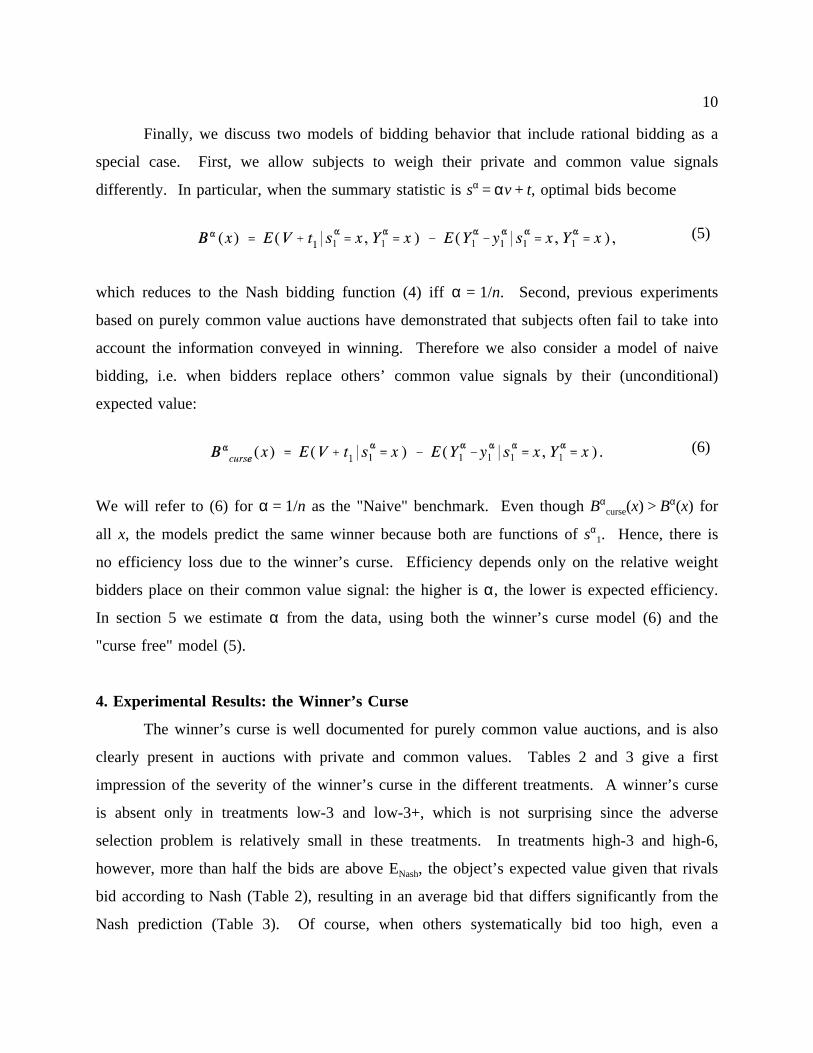
Finally, we discuss two models of bidding behavior that include rational bidding as a

special case. First, we allow subjects to weigh their private and common value signals

differently. In particular, when the summary statistic is sα = αv + t, optimal bids become

which reduces to the Nash bidding function (4) iff α = 1/n. Second, previous experiments

(5)

based on purely common value auctions have demonstrated that subjects often fail to take into

account the information conveyed in winning. Therefore we also consider a model of naive

bidding, i.e. when bidders replace others’ common value signals by their (unconditional)

expected value:

We will refer to (6) for α = 1/n as the "Naive" benchmark. Even though Bαcurse(x) > Bα(x) for

(6)

all x, the models predict the same winner because both are functions of sα1. Hence, there is

no efficiency loss due to the winner’s curse. Efficiency depends only on the relative weight

bidders place on their common value signal: the higher is α, the lower is expected efficiency.

In section 5 we estimate α from the data, using both the winner’s curse model (6) and the

"curse free" model (5).

4. Experimental Results: the Winner’s Curse

The winner’s curse is well documented for purely common value auctions, and is also

clearly present in auctions with private and common values. Tables 2 and 3 give a first

impression of the severity of the winner’s curse in the different treatments. A winner’s curse

is absent only in treatments low-3 and low-3+, which is not surprising since the adverse

selection problem is relatively small in these treatments. In treatments high-3 and high-6,

however, more than half the bids are above ENash, the object’s expected value given that rivals

bid according to Nash (Table 2), resulting in an average bid that differs significantly from the

Nash prediction (Table 3). Of course, when others systematically bid too high, even a

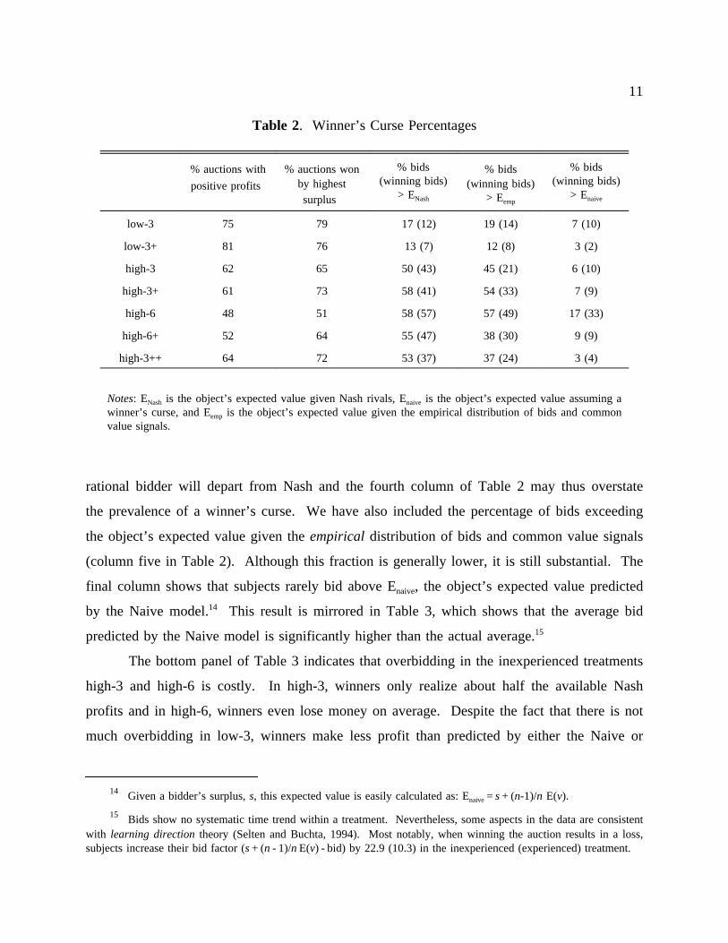
11

rational bidder will depart from Nash and the fourth column of Table 2 may thus overstate

Table 2. Winner’s Curse Percentages

% auctions with

positive profits

% auctions wonby highestsurplus

% bids(winning bids)

> ENash

% bids(winning bids)

> Eemp

% bids(winning bids)

> Enaive

low-3 75 79 17 (12) 19 (14) 7 (10)

low-3+ 81 76 13 (7) 12 (8) 3 (2)

high-3 62 65 50 (43) 45 (21) 6 (10)

high-3+ 61 73 58 (41) 54 (33) 7 (9)

high-6 48 51 58 (57) 57 (49) 17 (33)

high-6+ 52 64 55 (47) 38 (30) 9 (9)

high-3++ 64 72 53 (37) 37 (24) 3 (4)

Notes: ENash is the object’s expected value given Nash rivals, Enaive is the object’s expected value assuming awinner’s curse, and Eemp is the object’s expected value given the empirical distribution of bids and commonvalue signals.

the prevalence of a winner’s curse. We have also included the percentage of bids exceeding

the object’s expected value given the empirical distribution of bids and common value signals

(column five in Table 2). Although this fraction is generally lower, it is still substantial. The

final column shows that subjects rarely bid above Enaive, the object’s expected value predicted

by the Naive model.14 This result is mirrored in Table 3, which shows that the average bid

predicted by the Naive model is significantly higher than the actual average.15

The bottom panel of Table 3 indicates that overbidding in the inexperienced treatments

high-3 and high-6 is costly. In high-3, winners only realize about half the available Nash

profits and in high-6, winners even lose money on average. Despite the fact that there is not

much overbidding in low-3, winners make less profit than predicted by either the Naive or

14 Given a bidder’s surplus, s, this expected value is easily calculated as: Enaive = s + (n-1)/n E(v).

15 Bids show no systematic time trend within a treatment. Nevertheless, some aspects in the data are consistentwith learning direction theory (Selten and Buchta, 1994). Most notably, when winning the auction results in a loss,subjects increase their bid factor (s + (n - 1)/n E(v) - bid) by 22.9 (10.3) in the inexperienced (experienced) treatment.

12

Nash benchmark. This is because the auction is not always won by the bidder with the

Table 3. Bids and the Winner’s CurseTop Panel: Bids, Lower Panel: Winner’s Profit Per Period

low-3 high-3 high-6 low-3+ high-3+ high-6+ high-3++

Actual 189.6 172.6 182.4 189.5 179.5 176.7 175.6

Naive 191.50.09

186.70.01

194.30.01

191.50.12

187.00.05

194.60.11

187.00.02

Nash 188.30.28

159.90.01

171.10.01

188.30.17

160.40.03

169.30.29

160.70.02

ENash 197.10.01

173.90.51

176.40.01

197.10.03

174.50.05

174.31.00

174.80.87

Actual 7.27 11.88 -2.75 9.62 10.55 5.34 12.44

Naive 12.020.01

8.540.33

2.670.02

11.720.05

8.830.17

2.230.29

9.310.05

Nash 13.340.01

21.770.01

10.010.01

13.050.03

21.960.03

9.830.11

22.450.02

Notes: The p-value of a Wilcoxon rank test comparing predictions of the benchmark models with the actual bidare displayed in italics. Groups are the unit of observation. Test results are based on only three pair-wiseobservations in high-6+. ENash is the object’s expected value given Nash rivals.

highest surplus (see Table 2), as predicted by Nash/Naive bidding. One possible explanation

for why a bidder with an inferior surplus wins the auction is that subjects put too much

weight on their common value signal. An alternative explanation is that bidding is more

erratic or "noisy" (see section 6).

Overall, subjects’ performance is somewhat better in the experienced sessions than in

the inexperienced sessions. First, in the inexperienced sessions 7 subjects (6%) went

bankrupt, while none of the experienced subjects went bankrupt. Second, earnings are higher

in the experienced sessions. This improved performance may be either the result of learning,

selection, or both. Subjects that subscribed for an experienced session earned, on average,

1.62 points per period in the inexperienced sessions, while those that did not subscribe earned

1.03 points. This supports the idea that selection plays a role, although the difference

between the earnings is far from significant (a Mann-Whitney test with subjects as the unit of

observation yields p = 0.77). The 45 subjects that participated twice in the same treatment

13

earned somewhat higher profits and deviated slightly less from Nash (in an absolute sense) in

the experienced session. Thus, there are also some (weak) signs for learning, although

learning mainly occurs within the inexperienced session, and not between the inexperienced

and experienced sessions.

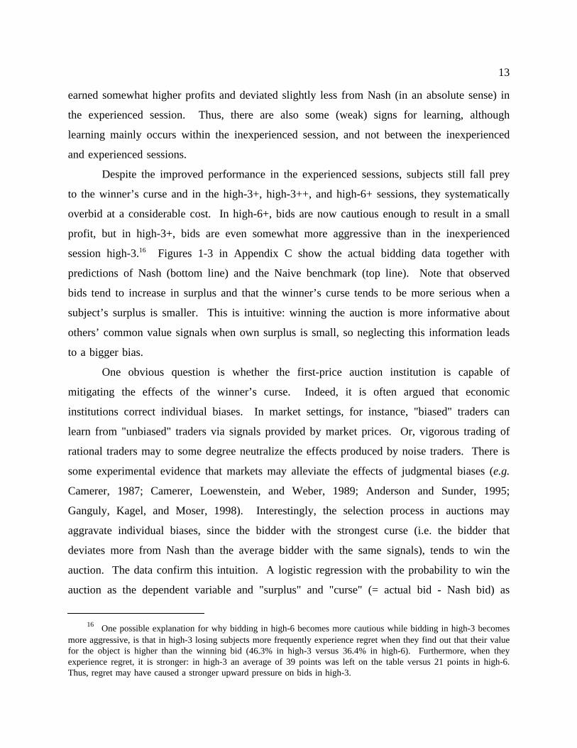
Despite the improved performance in the experienced sessions, subjects still fall prey

to the winner’s curse and in the high-3+, high-3++, and high-6+ sessions, they systematically

overbid at a considerable cost. In high-6+, bids are now cautious enough to result in a small

profit, but in high-3+, bids are even somewhat more aggressive than in the inexperienced

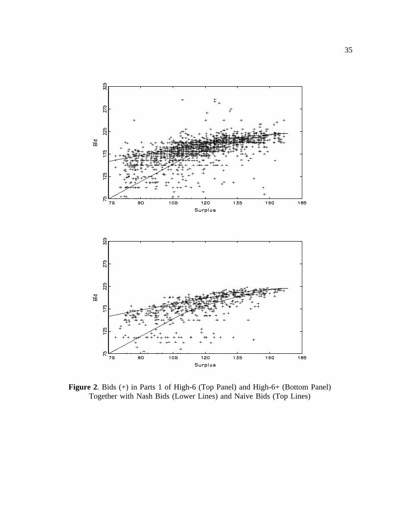
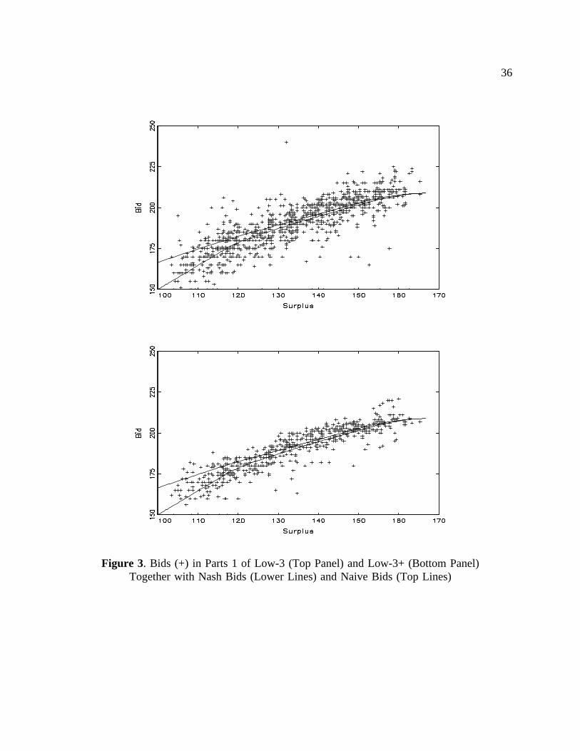
session high-3.16 Figures 1-3 in Appendix C show the actual bidding data together with

predictions of Nash (bottom line) and the Naive benchmark (top line). Note that observed

bids tend to increase in surplus and that the winner’s curse tends to be more serious when a

subject’s surplus is smaller. This is intuitive: winning the auction is more informative about

others’ common value signals when own surplus is small, so neglecting this information leads

to a bigger bias.

One obvious question is whether the first-price auction institution is capable of

mitigating the effects of the winner’s curse. Indeed, it is often argued that economic

institutions correct individual biases. In market settings, for instance, "biased" traders can

learn from "unbiased" traders via signals provided by market prices. Or, vigorous trading of

rational traders may to some degree neutralize the effects produced by noise traders. There is

some experimental evidence that markets may alleviate the effects of judgmental biases (e.g.

Camerer, 1987; Camerer, Loewenstein, and Weber, 1989; Anderson and Sunder, 1995;

Ganguly, Kagel, and Moser, 1998). Interestingly, the selection process in auctions may

aggravate individual biases, since the bidder with the strongest curse (i.e. the bidder that

deviates more from Nash than the average bidder with the same signals), tends to win the

auction. The data confirm this intuition. A logistic regression with the probability to win the

auction as the dependent variable and "surplus" and "curse" (= actual bid - Nash bid) as

16 One possible explanation for why bidding in high-6 becomes more cautious while bidding in high-3 becomesmore aggressive, is that in high-3 losing subjects more frequently experience regret when they find out that their valuefor the object is higher than the winning bid (46.3% in high-3 versus 36.4% in high-6). Furthermore, when theyexperience regret, it is stronger: in high-3 an average of 39 points was left on the table versus 21 points in high-6.Thus, regret may have caused a stronger upward pressure on bids in high-3.

14

independent variables, shows that the estimated parameter for surplus is 0.10 (s.d. 0.003), the

estimated parameter for curse is 0.06 (s.d. 0.003) and the estimated parameter for the constant

is -14.45 (s.d. 0.443). Hence, subjects with a stronger curse have a higher probability to

determine the price for the commodity.17

5. Experimental Results: Efficiency

Recall from section 3 that the relative weight bidders place on their common value

signal determines the efficiency level of the auction. For example, if bidders would ignore

their common value information, bids are ranked according to the private value signals, and

100% efficiency is attained. At the other extreme case where bidders neglect their private

information, the auction is no more efficient than a random allocation rule. For Nash and

Naive bidders, the weight of the common value signal is 1/n, which results in an intermediate

level of inefficiency.

Table 4 shows the efficiency levels realized in the experiment, per block of ten

periods, and the predictions of several benchmark models are added for comparison. The

efficiency levels are determined as follows. Let twinner denote the private value of the winner

and tmin (tmax) the minimal (maximal) private value in the group, then

The efficiency level predicted by a benchmark is obtained by replacing twinner with the private

(7)

value of the bidder predicted to win by the model. The predicted efficiencies of the Nash and

Naive benchmarks are the same since both models predict the same winner.

Note that actual efficiency levels are substantially below the Nash/Naive predictions in

the first ten periods of the inexperienced sessions, although this difference becomes smaller in

later periods. The efficiency levels of the experienced treatments are roughly constant and in

the same range as those in the last twenty periods of the inexperienced sessions. In the next

17 This selection force may weaken in the long run, however, as bidders with more severe curses go bankruptand disappear from the auctions.

15

section we compare the benchmarks of section 3 to the individual data.

Table 4. Observed Efficiencies By Blocks of Ten Periods

inexperienced once experienced twice experienced

1-10 11-20 21-30 1-10 11-20 21-30 1-10 11-20 21-30

High-3High-3 High-3+High-3+ High-3++High-3++

Actual 54 68 68 73 62 72 71 69 71

Nash/Naive 710.01

730.07

750.07

720.92

720.05

750.12

750.46

730.31

760.18

High-6High-6 High-6+High-6+

Actual 72 81 85 93 89 90

Nash/Naive 940.01

860.05

910.07

921.00

881.00

911.00

Low-3Low-3 Low-3+Low-3+

Actual 79 87 89 90 91 86

Nash/Naive 960.01

930.11

980.01

970.03

920.92

970.04

Notes: The p-value of a Wilcoxon rank test comparing a model’s efficiency with realized efficiency isdisplayed in italics. Groups are the unit of observation.

6. Analysis of the Individual Bidding Data

The Nash and Naive benchmark both make point predictions, and one has to make an

assumption about how players err to evaluate these models. We invoke a commonly made

assumption: for each of the benchmarks a random error term is added to the predicted bid.

The error terms are drawn from a truncated Normal distribution with mean 0 and variance σ2,

and are identically and independently distributed across subjects and periods.18 This method

of transforming deterministic models into stochastic models can easily be criticized on

theoretical grounds, but there is no a priori reason why one model will be favored over

another. So this procedure seems adequate to compare the "goodness-of-fit" of different

benchmark models. Since the results of the previous section suggest a difference between

18 The distribution is truncated to ensure that bids stay between the lower and upper limit on bids.

16

bidding behavior in the first ten and later periods (see Table 4), we provide separate tables for

Table 5A. Maximum Likelihood Results for Periods 11-30

low-3n=600

high-3n=519

high-6n=981

low-3+n=360

high-3+n=360

high-6+n=360

high-3++n=420

Nash σ 8.4 25.4 27.9 6.4 28.1 31.0 26.2

-logL 3.53 4.60 4.71 3.26 4.70 4.79 4.64

Naive σ 8.8 21.9 26.2 7.0 18.5 34.3 23.2

-logL 3.59 4.50 4.68 3.37 4.34 4.95 4.56

Nash - NaiveCombined

σ1 6.0 21.4 27.6 4.9 27.3 30.6 23.8

σ2 15.5 15.8 12.5 10.4 12.9 8.8 12.7

p 0.83 0.45 0.44 0.77 0.22 0.72 0.37

-logL 3.38 4.32 4.31 3.20 4.15 4.49 4.21

Bα - Bαcurse

Combined

σ1 5.6 21.9 27.6 4.8 20.3 30.7 25.3

σ2 13.4 15.9 12.6 10.6 13.8 8.8 12.2

p 0.75 0.32 0.44 0.78 0.11 0.72 0.33

α 0.40 0.47 0.17 0.28 0.43 0.17 0.42

-logL 3.37 4.30 4.31 3.19 4.10 4.49 4.18

Random -logL 4.62 5.53 5.53 4.62 5.53 5.53 5.53

Notes: Loglikelihood per choice is displayed.

periods 1-10 and periods 11-30.

Table 5A reports the estimation results for the final twenty periods. The top panel

pertains to the Nash and Naive benchmarks. Based on the loglikelihoods there is no obvious

ranking of the two models: Nash performs better in low-3, Naive in high-3, and the results

are mixed for high-6. Glancing at Figures 1-3, it seems plausible that there is some

heterogeneity among subjects, with some bidders suffering from the winner’s curse while

others don’t. This is tested in the Nash-Naive combined model, which allows subjects to bid

17

according to either the Nash or Naive benchmark.19 This combined model results in a much

higher likelihood than either of the two individual models.

The Nash-Naive combined model should be compared to the model in the bottom

panel of Table 5A, which is based on the bidding functions (5) and (6). This model also

allows (a fraction of the) bidders to fall prey to the winner’s curse, and to weigh their

common value signal differently than Nash bidders (i.e. the relative weight of the common

value signal is not necessarily 1/n). The inclusion of the weight α results in a small, albeit

significant increase in likelihood when there are three bidders, but adds nothing when group

size is six. The maximum likelihood results suggest that while a significant fraction of the

subjects (e.g. more than 50 percent) falls prey to a winner’s curse, bidders correctly weigh

their private and common value information. This conclusion, which is based on the

individual bidding data, is further corroborated by the aggregate results of Table 4, which

shows that actual efficiency levels are close to predicted levels in the final part. To

summarize, the data seem best described by a model in which bidders weigh their information

in roughly the same manner as rational bidders would, while a fraction of the bidders falls

prey to the winner’s curse.20

Estimates for the initial ten periods of the different treatments are reported in Table

5B. For the inexperienced treatments, all models result in much lower likelihoods than those

reported for the final twenty periods (Table 5A). This is partly due to the higher weight

bidders assign to their common value signal, which causes the "wrong" bidder to win.

19 To be precise, the unconditional likelihood L(xi,11,...,xi,30) of a player i’s choices x in periods 11-30 is:

where L(xi,t|Nash) represents the conditional probability of xi,t predicted by the Nash model, L(xi,t|Naive) represents theconditional probability of xi,t given the Naive model, and p is the probability that a subject plays according to theNash equilibrium. The Nash and Naive benchmarks are nested as special cases (i.e. p = 1 or p = 0).

20 We also estimated a model in which bidders make a "logit" best response to the empirical distribution of bids(with or without a winner’s curse). This model generally resulted in a much worse description of the data (i.e. a 10-20 percent reduction in the loglikelihood per obervation). Finally, we estimated a "discount" model in which bids aredetermined as a fraction of the (rational or naive) expected value of the object. This model yielded similarloglikelihoods as the ones in Table 5. We prefer the benchmark models of section 3, however, as they have a moresound theoretical foundation.

18

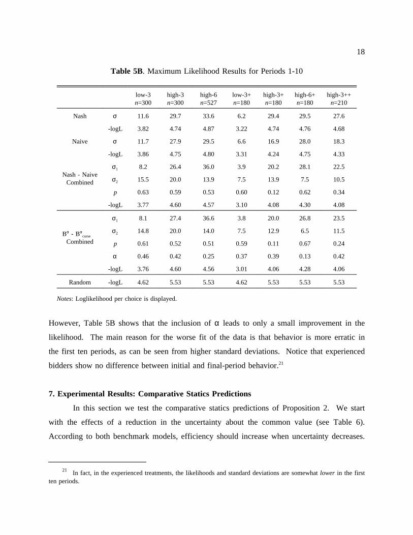
However, Table 5B shows that the inclusion of α leads to only a small improvement in the

Table 5B. Maximum Likelihood Results for Periods 1-10

low-3n=300

high-3n=300

high-6n=527

low-3+n=180

high-3+n=180

high-6+n=180

high-3++n=210

Nash σ 11.6 29.7 33.6 6.2 29.4 29.5 27.6

-logL 3.82 4.74 4.87 3.22 4.74 4.76 4.68

Naive σ 11.7 27.9 29.5 6.6 16.9 28.0 18.3

-logL 3.86 4.75 4.80 3.31 4.24 4.75 4.33

Nash - NaiveCombined

σ1 8.2 26.4 36.0 3.9 20.2 28.1 22.5

σ2 15.5 20.0 13.9 7.5 13.9 7.5 10.5

p 0.63 0.59 0.53 0.60 0.12 0.62 0.34

-logL 3.77 4.60 4.57 3.10 4.08 4.30 4.08

Bα - Bαcurse

Combined

σ1 8.1 27.4 36.6 3.8 20.0 26.8 23.5

σ2 14.8 20.0 14.0 7.5 12.9 6.5 11.5

p 0.61 0.52 0.51 0.59 0.11 0.67 0.24

α 0.46 0.42 0.25 0.37 0.39 0.13 0.42

-logL 3.76 4.60 4.56 3.01 4.06 4.28 4.06

Random -logL 4.62 5.53 5.53 4.62 5.53 5.53 5.53

Notes: Loglikelihood per choice is displayed.

likelihood. The main reason for the worse fit of the data is that behavior is more erratic in

the first ten periods, as can be seen from higher standard deviations. Notice that experienced

bidders show no difference between initial and final-period behavior.21

7. Experimental Results: Comparative Statics Predictions

In this section we test the comparative statics predictions of Proposition 2. We start

with the effects of a reduction in the uncertainty about the common value (see Table 6).

According to both benchmark models, efficiency should increase when uncertainty decreases.

21 In fact, in the experienced treatments, the likelihoods and standard deviations are somewhat lower in the firstten periods.

19

The intuition is that with less variation in the common value signal, vi, private value

Table 6. Effect of Uncertainty about the Common ValueTop Panel: Efficiency, Middle Panel: Winner’s Profit, Bottom Panel: Revenues

Inexperienced Experienced

high-3 low-3 p-value high-3+ low-3+ p-value

Actual 62 85 0.00 69 89 0.00

Nash/Naive 73 96 0.00 73 95 0.00

Actual 11.88 7.27 0.27 10.55 9.62 0.38

Nash 21.77 13.34 0.00 21.96 13.05 0.00

Naive 8.54 12.02 0.10 8.83 11.72 0.52

Actual 194.1 202.4 0.03 198.2 200.8 0.20

Nash 187.0 198.7 0.00 187.2 198.5 0.00

Naive 200.2 200.1 0.94 200.4 199.9 0.69

Notes: The third and the sixth column report p-values for a Mann-Whitney rank test results comparing high-3with low-3 and low-3+ and high-6+ respectively. Groups are the unit of observation.

differences are exemplified, making it more likely that the bidder with the highest private

value wins. This predicted effect of a decrease in uncertainty is borne out by the data: the

realized efficiency level is substantially and significantly higher in treatment low-3 than in

high-3, both for inexperienced and experienced subjects.

The effect of increased uncertainty on winner’s profits and revenues depends on the

benchmark. Nash predicts that with more uncertainty, bids are less aggressive because of the

increased winner’s curse and profits are higher as a result. In contrast, naive bidders neglect

the fact that winning is informative and hence are insensitive to the increased risk of a

winner’s curse. In fact, they will bid higher when there is more uncertainty, because the

maximum surplus, v/n + t, is higher when the common value signals are drawn from U[0,200]

than when they are drawn from U[75,125]. Table 6 shows that actual profits are lower with

less uncertainty, although less so than predicted by Nash (both for inexperienced and

experienced bidders). Revenue results are the opposite: Nash predicts that revenues will

decrease when the uncertainty about the common value increases, while the naive benchmark

20

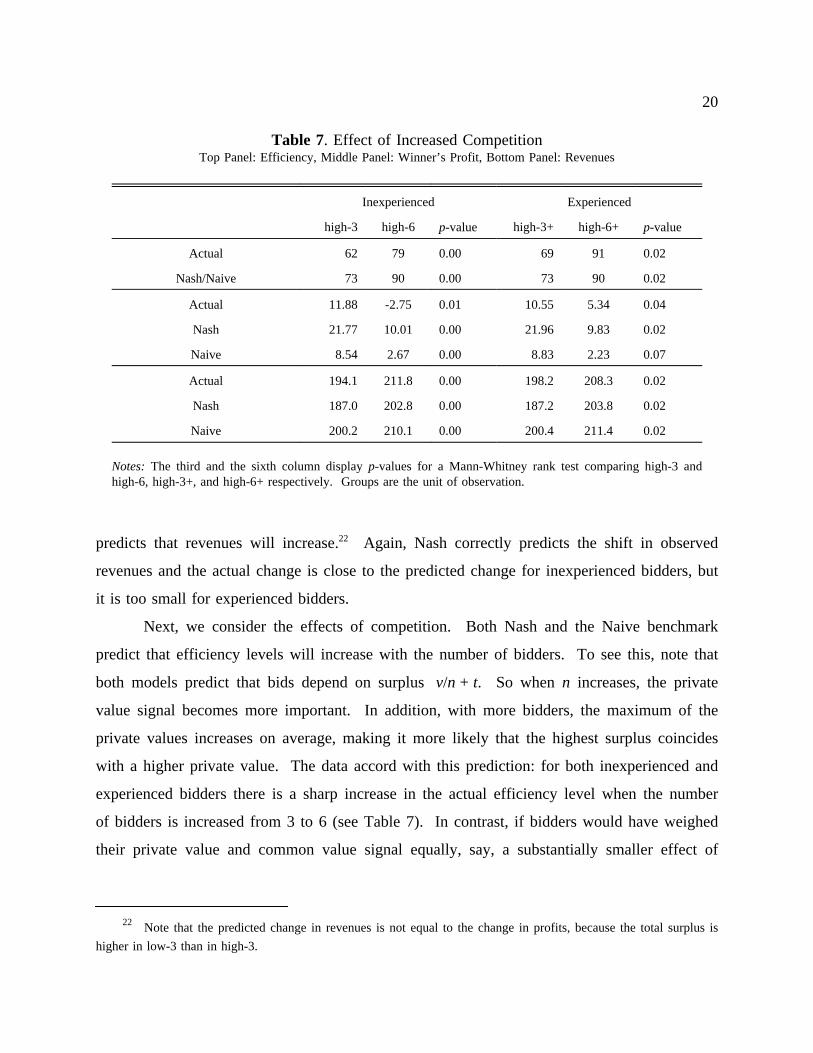
predicts that revenues will increase.22 Again, Nash correctly predicts the shift in observed

Table 7. Effect of Increased CompetitionTop Panel: Efficiency, Middle Panel: Winner’s Profit, Bottom Panel: Revenues

Inexperienced Experienced

high-3 high-6 p-value high-3+ high-6+ p-value

Actual 62 79 0.00 69 91 0.02

Nash/Naive 73 90 0.00 73 90 0.02

Actual 11.88 -2.75 0.01 10.55 5.34 0.04

Nash 21.77 10.01 0.00 21.96 9.83 0.02

Naive 8.54 2.67 0.00 8.83 2.23 0.07

Actual 194.1 211.8 0.00 198.2 208.3 0.02

Nash 187.0 202.8 0.00 187.2 203.8 0.02

Naive 200.2 210.1 0.00 200.4 211.4 0.02

Notes: The third and the sixth column display p-values for a Mann-Whitney rank test comparing high-3 andhigh-6, high-3+, and high-6+ respectively. Groups are the unit of observation.

revenues and the actual change is close to the predicted change for inexperienced bidders, but

it is too small for experienced bidders.

Next, we consider the effects of competition. Both Nash and the Naive benchmark

predict that efficiency levels will increase with the number of bidders. To see this, note that

both models predict that bids depend on surplus v/n + t. So when n increases, the private

value signal becomes more important. In addition, with more bidders, the maximum of the

private values increases on average, making it more likely that the highest surplus coincides

with a higher private value. The data accord with this prediction: for both inexperienced and

experienced bidders there is a sharp increase in the actual efficiency level when the number

of bidders is increased from 3 to 6 (see Table 7). In contrast, if bidders would have weighed

their private value and common value signal equally, say, a substantially smaller effect of

22 Note that the predicted change in revenues is not equal to the change in profits, because the total surplus is

higher in low-3 than in high-3.

21

increasing competition would be expected (from 63% to 65% in high-6 and from 62% to 66%

in high-6+).

Both benchmarks yield identical predictions for the effects of an increase in the

number of bidders on profits and revenues. Revenues increase with the number of bidders for

two reasons. First, with more competition, bidders are forced to bid closer to their estimate

of the value of the commodity. Second, with a higher number of bidders the total surplus to

be divided between seller and bidders is higher. The opposite effect is expected for the

winner’s profits, which declines with more bidders according to both benchmarks. Table 7

shows that for both inexperienced and experienced bidders, the profit of the winning bidder

decreases as the number of bidders increases.

Finally, consider the case where the auctioneer has an independent estimate of the

common value of the object for sale. By revealing this information, the auctioneer decreases

bidders’ uncertainty about the common value, which results in a more efficient allocation.

The decrease in uncertainty reduces the winner’s curse, forcing bidders to be more aggressive,

resulting in lower winner’s profits and higher revenues.23 The higher the quality of the

auctioneer’s information, the stronger the predicted effects.

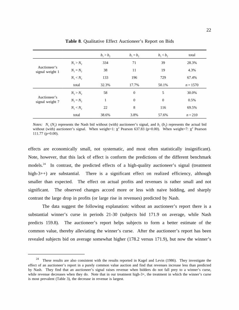
Table 8 shows that, by and large, bidders change their bid in the direction predicted by

Nash, both when the quality of the auctioneer’s signal is the same as that of the bidders and

when its quality is higher. Interestingly, the most common deviation from the Nash

prediction is that a bidder does not increase her bid when Nash bidders would. This occurs

when bidders neglect the fact that the extra information mitigates the winner’s curse and that,

as a consequence, more aggressive bidding is warranted.

Table 9 shows that the public disclosure of the auctioneer’s signal, which is of the

same quality as bidders’ signals, has no effects on efficiency, revenues, and profits (i.e. the

23 This argument is flawed when bidders neglect the fact that winning is informative. The disclosure of theauctioneer’s information leads to an improvement in bidders’ estimates of the value, resulting in a more efficientallocation. However, when bidders neglect the fact that winning is informative both with and without the auctioneer’sreport, their bids will be equally aggressive. Due to the improved estimate of the value, higher profits for the winnerare expected though. The effect of information disclosure on revenue is ambiguous, since the positive effect of ahigher winner’s curse without information may be offset by a negative effect on the total surplus to be dividedbetween the seller and the bidders.

22

effects are economically small, not systematic, and most often statistically insignificant).

Table 8. Qualitative Effect Auctioneer’s Report on Bids

b1 > b2 b1 = b2 b1 < b2 total

Auctioneer’ssignal weight 1

N1 > N2 334 71 39 28.3%

N1 = N2 38 11 19 4.3%

N1 < N2 133 196 729 67.4%

total 32.3% 17.7% 50.1% n = 1570

Auctioneer’ssignal weight 7

N1 > N2 58 0 5 30.0%

N1 = N2 1 0 0 0.5%

N1 < N2 22 8 116 69.5%

total 38.6% 3.8% 57.6% n = 210

Notes: N1 (N2) represents the Nash bid without (with) auctioneer’s signal, and b1 (b2) represents the actual bidwithout (with) auctioneer’s signal. When weight=1: χ2 Pearson 637.83 (p=0.00). When weight=7: χ2 Pearson111.77 (p=0.00).

Note, however, that this lack of effect is conform the predictions of the different benchmark

models.24 In contrast, the predicted effects of a high-quality auctioneer’s signal (treatment

high-3++) are substantial. There is a significant effect on realized efficiency, although

smaller than expected. The effect on actual profits and revenues is rather small and not

significant. The observed changes accord more or less with naive bidding, and sharply

contrast the large drop in profits (or large rise in revenues) predicted by Nash.

The data suggest the following explanation: without an auctioneer’s report there is a

substantial winner’s curse in periods 21-30 (subjects bid 171.9 on average, while Nash

predicts 159.8). The auctioneer’s report helps subjects to form a better estimate of the

common value, thereby alleviating the winner’s curse. After the auctioneer’s report has been

revealed subjects bid on average somewhat higher (178.2 versus 171.9), but now the winner’s

24 These results are also consistent with the results reported in Kagel and Levin (1986). They investigate theeffect of an auctioneer’s report in a purely common value auction and find that revenues increase less than predictedby Nash. They find that an auctioneer’s signal raises revenue when bidders do not fall prey to a winner’s curse,while revenue decreases when they do. Note that in our treatment high-3+, the treatment in which the winner’s curseis most prevalent (Table 3), the decrease in revenue is largest.

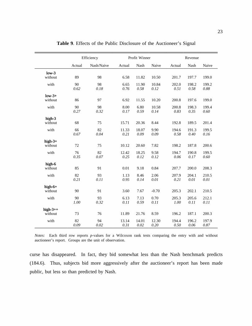
23

curse has disappeared. In fact, they bid somewhat less than the Nash benchmark predicts

Table 9. Effects of the Public Disclosure of the Auctioneer’s Signal

Efficiency Profit Winner Revenue

Actual Nash/Naive Actual Nash Naive Actual Nash Naive

low-3low-3without 89 98 6.58 11.82 10.50 201.7 197.7 199.0

with 900.62

980.18

6.650.76

11.900.58

10.840.12

202.00.51

198.20.58

199.20.88

low-3+low-3+without 86 97 6.92 11.55 10.20 200.8 197.6 199.0

with 900.27

980.32

8.000.17

6.800.59

10.580.14

200.80.83

198.30.35

199.40.60

high-3high-3without 68 75 15.71 20.36 8.44 192.8 189.5 201.4

with 660.67

820.04

11.330.21

18.070.09

9.900.09

194.60.58

191.30.40

199.50.16

high-3+high-3+without 72 75 10.12 20.60 7.82 198.2 187.8 200.6

with 760.35

820.07

12.420.25

18.250.12

9.580.12

194.70.06

190.80.17

199.50.60

high-6high-6without 85 91 0.01 9.18 0.84 207.7 200.0 208.3

with 820.21

930.11

1.130.95

8.460.14

2.060.01

207.90.21

204.10.01

210.50.01

high-6+high-6+without 90 91 3.60 7.67 -0.70 205.3 202.1 210.5

with 901.00

930.32

6.130.11

7.130.59

0.700.11

205.31.00

205.60.11

212.10.11

high-3++high-3++without 73 76 11.89 21.76 8.59 196.2 187.1 200.3

with 820.09

940.02

13.140.31

14.010.02

12.300.20

194.40.50

196.20.06

197.90.87

Notes: Each third row reports p-values for a Wilcoxon rank tests comparing the entry with and withoutauctioneer’s report. Groups are the unit of observation.

(184.6). Thus, subjects bid more aggressively after the auctioneer’s report has been made

public, but less so than predicted by Nash.

24

8. Conclusion

The majority of the theoretical and empirical literature on auctions pertains to either

private or common value auctions. A remarkable feature of these polar cases is that both

yield fully efficient allocations (in a Nash equilibrium). Most real-world auctions, however,

exhibit both private and common value elements and inefficiencies should be expected, even

in a Nash equilibrium. This paper reports a series of first-price auction experiments in which

bidders receive a private value signal and an independent common value signal. We

investigate the extent of inefficiency that occurs with (financially motivated) human bidders.

In addition, we test several policies aimed at reducing inefficiencies.

As expected, a fraction of the bidders falls prey to the winner’s curse and this curse is

more severe when winning is more informative. While there is systematical overbidding in

most treatments, bidders aggregate their private and common value information in roughly the

same manner as rational bidders would. As a result, realized efficiencies are of the same

magnitude as predicted by Nash. Large differences occur only in the first ten periods of the

inexperienced sessions, and seem mostly due to initially more erratic behavior. These

findings are further corroborated by an analysis of the individual bidding data.

An increase in uncertainty about the common value leads to a substantial decrease in

efficiency, accompanied by a slight increase in winner’s profits and a slight decrease in the

seller’s revenues. These results are in line with Nash predictions, although the effects on

profits and revenues are smaller than predicted because the increase in uncertainty aggravates

the winner’s curse. The public disclosure of the auctioneer’s information about the common

value has no systematic effects on efficiency, profits, or revenues when the information

provided is of the same quality as that of the bidders. Furthermore, the public release of

high-quality information positively affects efficiency, although less so than predicted by Nash.

Finally, our results indicate that more competition is a robust way to enhance

efficiency, reduce winner’s profits, and raise the seller’s revenues. The reasons for these

positive effects are partly "statistical": with more bidders, the winner will on average have

better information (i.e. higher signals). More importantly, however, an increase in

competition induces bidders to weigh their own common value signal significantly less, which

makes their private value information more important and an efficient outcome more likely.

25

ReferencesAbbink, Klaus and Abdolkarim Sadrieh (1995) "Ratimage, Research Assistance Toolbox for

Computer-Aided Human Behavior Experiments," Discussion paper B-325, Universityof Bonn.

Albers, Wulf and Ronald M. Harstad (1991) "Common-Value Auctions with IndependentInformation: A Framing Effect Observed in a Market Game," in R. Selten, ed., GameEquilibrium Models: Volume II, Berlin: Springer-Verlag.

Anderson, M.J., and S. Sunder (1995) "Professional Traders as Intuitive Bayesians," Organi-zational Behavior and Human Decision Processes, 64, 185-202.

Ashenfelter, Orley and David Genesove (1992), "Testing for Price Anomalies in Real-EstateAuctions," American Economic Review: Papers and Proceedings, 82, 501-5.

Avery, Christopher and John H. Kagel (1997), "Second-Price Auctions with AsymmetricPayoffs: An Experimental Investigation," Journal of Economics and ManagementStrategy, 6(3), 573-603.

Bazerman, Max H. and William F. Samuelson (1983), "I Won the Auction But Don’t Wantthe Prize," Journal of Conflict Resolution, 27(4), 618-34.

Bikhchandani, Sushil and John G. Riley (1991) "Equilibria in Open Common Value Auc-tions," Journal of Economic Theory, 53, 101-130.

Bulow, Jeremy I. and Paul D. Klemperer (1999) "Prices and the Winner’s Curse," workingpaper.

Bulow, Jeremy I., M. Huang and Paul D. Klemperer (1999) "Toeholds and Takeovers,"Journal of Political Economy, 107(3), 427-54.

Camerer, Colin F. (1987) "Do Biases in Probability Judgments Matter in Markets? Experi-mental Evidence," American Economic Review, 77, 981-997.

Camerer, C., G. Loewenstein, and M. Weber (1989) "The Curse of Knowledge in EconomicSettings: An Experimental Analysis," Journal of Political Economy, 97, 1232-1254.

Capen E.C., R.V. Clapp and W.M. Campbell (1971), "Competitive Bidding in High-RiskSituations," Journal of Petroleum Technology, 23, 641-53.

Campbell, Colin M., John H. Kagel and Dan Levin (1999), "The Winner’s Curse and PublicInformation in Common Value Auctions: Reply," American Economic Review, 89,325-334.

Cox, James C., Samuel H. Dinkin and Vernon L. Smith (1998), "Endogenous Entry and Exitin Common Value Auctions," working paper, University of Arizona.

Cox, James C., Samuel H. Dinkin and Vernon L. Smith (1999), "The Winner’s Curse andPublic Information in Common Value Auctions: Comment," American EconomicReview, 89, 319-324.

Dasgupta, Partha and Eric S. Maskin (1999) "Efficient Auctions," Quarterly Journal ofEconomics, forthcoming.

Dyer, Douglas, John H. Kagel and Dan Levin (1989), "A Comparison of Naive and Experi-enced Bidders in Common Value Offer Auctions," Economic Journal, 99, 108-15.

Ganguly, A.R., J.H. Kagel, and D.V. Moser (1998) "Do Asset Market Prices Reflect Traders’Judgment Biases?," working paper, University of Pittsburgh.

Garvin, Susan and John H. Kagel (1994), "Learning in Common Value Auctions: Some InitialObservations," Journal of Economic Behavior and Organization, 25, 351-72.

26

Goeree, Jacob K. and Theo Offerman (1999), "Competitive Bidding in Auctions with Privateand Common Values," working paper, University of Virginia.

Jehiel, Philippe and Benny Moldovanu (1999) "Efficient Design with Interdependent Valua-tions," working paper, Mannheim University.

Holt, Charles A. and Roger Sherman (2000) "Risk Aversion and the Winner’s Curse,"Working Paper, University of Virginia.

Kagel, John H., Ronald M. Harstad and Dan Levin (1987), "Information Impact andAllocation Rules in Auctions with Affiliated Private Values: A Laboratory Study,"Econometrica, 55, 1275-1304.

Kagel, John H. and Dan Levin (1986), "The Winner’s Curse and Public Information inCommon Value Auctions," American Economic Review, 76, 894-920.

Kagel, John H. and Dan Levin (1999), "Common Value Auctions with Insider Information,"Econometrica, 67(5), 1219-38.

Kagel, John H., Dan Levin, Raymond C. Battalio and Donald J. Meyer (1989), "First-PriceCommon Value Auctions: Bidder Behavior and the Winner’s Curse," EconomicInquiry, 27, 241-58.

Kirchkamp, Oliver and Benny Moldovanu (2000) "An Experimental Analysis of AuctionsWith Interdependent Valuations," Working Paper, University of Mannheim.

Klemperer, Paul D. (1998) "Auctions With Almost Common Values," European EconomicReview, 42, 757-769.

Krishna, Vijay and John Morgan (1997) "(Anti-) Competitive Effects of Joint Bidding andBidder Restrictions," working paper, Penn State University and Princeton University.

Levin, Dan, John H. Kagel and Jean-Francois Richard (1996), "Revenue Effects and Informa-tion Processing in English Common Value Auctions," American Economic Review, 86,442-60.

Lind, Barry and Charles R. Plott (1991), "The Winner’s Curse: Experiments with Buyers andwith Sellers," American Economic Review, 81(1), 335-46.

Maskin, Eric S. (1992) "Auctions and Privatization," in Privatization (ed. by H. Siebert),Institut fur Weltwirtschaften der Universitat Kiel, 115-136.

McAfee, Preston R. and John McMillan (1987) "Auctions and Bidding," Journal of EconomicLiterature, XXV(2), 699-738.

Pesendorfer, Wolfgang and Jeroen M. Swinkels (1999) "Efficiency and Information Aggrega-tion in Auctions," American Economic Review, forthcoming.

Roll, Richard (1986) "The Hubris Hypothesis of Corporate Takeovers," Journal of Business,59(2), 197-216.

Selten, Reinhard and Joachim Buchta (1994) "Experimental Sealed Bid First-Price Auctionswith Directly Observed Bid Functions," Discussion paper B-270, University of Bonn.

Stigler, George J. (1987) "Competition" in The New Palgrave: A Dictionary of Economics,edited by John Eatwell, Murray Milgate and Peter Newman. The Macmillan PressLimited: London.

Thaler, Richard H. (1988) "Anomalies: The Winner’s Curse," Journal of Economic Perspec-tives, 2(1), 191-202.

Wilson, Robert (1977) "A Bidding Model of Perfect Competition," Review of EconomicStudies, 44, 551-518.

27

Appendix A: (Computerized) Instructions for Treatment High-3Welcome to the experiment! You can make money in this experiment. Your choices willdetermine how much money you will make. Read the instructions carefully. There is paper,a pen, and a calculator on your table. You can use these during the experiment. Before theexperiment starts, we will hand out a summary of the instructions and there will be onepractice period.

The experimentThe experiment consists of two parts. You will earn points in both parts of the experiment.At the end of the experiment your points will be exchanged in guilders. Each point will yield25 cent. First you will receive the instructions for part 1. When part 1 of the experiment isfinished, you will receive the instructions for part 2.

Instructions part 1You will start part 1 with a starting capital of 120 points. Part 1 consists of 20 periods.Each period you will be allocated to a group of 3 persons. A product will be sold in yourgroup in each period. The person with the highest bid in the group will buy the product. Ifmore than one person choose the same highest bid, the computer will determine by lotterywhich participant will buy the product.

The buyer will not literally receive a product. He or she will receive an amount equalto the value of the product minus the costs of the product (in points).

Value and costs of the productThe participant who buys the product will pay a price equal to the own bid. The costs of theproduct are thus equal to the own bid.

The value of the product is determined as follows. For each participant the value isequal to a “private value” plus a “common value”. For each participant the private value willlie between 75 and 125 points, and each number between 75 and 125 is equally likely. Theprivate value of one participant is independent of the private value of the other participants.Your private value therefore (very) probably differs from those of the others. At the start ofa period you will get to know your private value. You will not know the private value ofother participants, just like other participants will not know your private value.

The common value of the product is determined as follows. Each participant in thegroup will receive a common component. A common component lies between 0 and 200points. The common component of the one participant is independent of the commoncomponents of the other participants. At the start of a period each participant will only get toknow her or his own common component. The COMMON VALUE equals the AVERAGEof the common components of the participants in a group. If the average is not an integer, itwill be rounded to the nearest integer. For each participant, all values between 0 and 200 areequally likely to be the common component.

Notice that the private value differs for each participant, while the common value isexactly the same for all members of the group. You know your private value at the time ofbidding. You will only know your own common component at the time of bidding. You will

28

not know the common value for sure, because you don't know others’ common valuecomponents. Thus at the time of bidding you only partially know the value of the product.

ProfitOnly the person with the highest bid earns an amount, which equals his or her private valueplus the common value minus his or her own bid. Notice that this amount may be negative.If the highest bidder bids higher than the value of the product, (s)he will make a loss. Justlike a profit is automatically added to the amount earned up to that period, a loss willautomatically be subtracted.

Note also that in the most unfavorable case the value of the product will equal 75points, when the common value equals 0 points and your private value equals 75 points. Inthe most favorable case the value of the product will equal 325 points, when the commonvalue equals 200 points and your private value equals 325 points. This is the reason that yourbid will have to lie between 75 and 325 points. Note: In low-3 and low-3+ bids wererestricted to [150, 250].

InformationWhen all bidders have entered their bid in a period, the results of the period will becommunicated. You will get to know all bids in your group, ordered from high to low. Youwill be told whether you did or did not buy the product. You will get to know the commonvalue of the product and your profit.

Then a new period will be started. In the new period again a product will be sold.For each participant the product will have a different value. Each participant receives a newprivate value for the product and a new common component. Your value for the product in aperiod will thus not depend on your value for the product in any other period.

Now you are asked to answer some questions about the instructions.

Question about the common valueAssume that your common component equals 112 points and you don't know the commoncomponents of the other participants. Assume that for the other participants it holds that:

Participant Common component1 1322 55

How large is the common value in this example?

Note: Subjects could only pass a question by giving the right answer. After a wrong answerthe relevant part in the instructions was explained anew, and the subject had to try again.

Question about the profitAssume that your private value for the product equals 115 points. The common value of theproduct in your group equals 87 points. You have bid 170 points (this bid is arbitrarily

29

chosen by us, and does not contain any information about how you should bid). Assume thatyour bid is the highest. How large is your profit in this case?

EndYou have reached the end of the instructions. If you want to read some parts of theinstructions again, push the button BACK.

Otherwise you push the button READY. When all participants have pushed READY,the experiment will start. When the experiment has started, you will not be able to return tothese instructions. Before the experiment is started, a summary of the instructions will behanded out and a practice period will be carried out. Your profit or loss during the practiceperiod will NOT be added to your earnings.

If you have a question, please raise your hand!

Instructions part 2Here follow the instructions for part 2. Before part 2 actually starts, you will receive

a summary of these instructions. An amount of 60 points will be added to the total that youearned until now. This is resulting amount is your starting capital for part 2. Part 2 lastsfrom period 21 to 30. Each period you will be allocated to a group of 3 persons, and oneproduct will be sold to each group.

Two decisions per periodFrom now on you will make two decisions per period. Each period consists of part A

and part B. In each part you make a decision. Only one of the two decisions will be actuallypaid. At the end of the period the computer determine by lottery which decision is paid out.The probability that decision A will be paid out is 50%. If decision A is not paid out,decision B will be paid out.

The decision that you will make in part A is exactly the same as the decision in thefirst part of the experiment.

Decision part BWhen all participants have made their decision for part A, part B of a period is

started. In part B each participant will again bid for the product. For a large part thesituation is the same as for the decision in part A. Again each participant is allocated to agroup of 3 persons. Again the product will be sold to the person with the highest bid. Withmore than one highest bid, the buyer will be determined by lottery. The buyer pays a priceequal to the own bid.

The value of the product in part B equals a private value plus a common value. Foreach participant the private value equals the private value in part A. The common componentis also for each participant exactly as the common component in part A. The only differencebetween the decision in part A and the decision in part B is that the common value for theproduct is computed differently.

The so-called PUBLIC COMPONENT is important for calculating the common valuein part B. The public component lies between 0 points and 200 points, where each number isequally likely. The value for the public component does not depend on the value of the

30

common components of the participants. EACH participant gets to know the publiccomponent of her or his group at the start of part B. Thus all participants in a group areconfronted with the same public component.

In part B the common value equals the AVERAGE of the common components of theparticipants in a group AND the public component of the group. To be precise, all commoncomponents of the participants in the group are added. Then the public component is addedto this number. The resulting number is divided by four and (when needed) rounded to theclosest integer number.

ProfitWhen all participants have made their decision for part B, the computer determines

whether part A or part B is used for actual payment. Only the person with the highest bid inthe part that is paid out earns an amount. This amount equals her or his private value plusthe common value minus her or his bid. Just like in the first part of the experiment profits(losses) are automatically added (subtracted) from the amount earned up to now.

You do not have to enter the same bid twice. Nor do you have to enter a different bidfor part B than for part A. It is up to you to decide what you want to do.

InformationWhen all participants have made both decisions, the results of the period will be

communicated. Only the results of the part that is used for actual payment will becommunicated. You will see all bids in your group ranked from high to low. You will get toknow whether or not you bought the product. You will see the common value of the productand your profit.

Then a new period will be started. In the new period again a product will be sold.For each participant the product will have a different value. Each participant receives a newprivate value for the product and a new common component. At the start of part B eachparticipant will see the new public component. Your value for the product in one period doesnot depend on your value for the product in any other period.

Now you will be asked to answer some questions about these instructions.

Question about the common valueAssume that your common component equals 54 points. The public component equals 113points. Assume that for the other participants it holds that:

Participant Common component1 1272 66

How large is the common value in this example?

Note: Again, subjects could only pass the question by giving the right answer. After a wronganswer the relevant part in the instructions was explained anew, and the subject had to tryagain.

31

Question about the public componentIs the following statement right or wrong?In part B of a period each participant in a group will receive a different public component.

EndYou have reached the end of the instructions. If you want to read some parts of theinstructions again, push the button BACK.

Otherwise you push the button READY. When all participants have pushed READY,the second part of the experiment will start. When the experiment has started, you will notbe able to return to these instructions. Before the experiment is started, a summary of theinstructions will be handed out.

If you have a question, please raise your hand!

32

Appendix B: Nash Equilibrium Bids for Treatment High-3

Recall from section 3 that the Nash equilibrium bids are given by

where the surplus variable is defined as s = v/n + t, and Y1 is the maximum of the n surplus

(B1)

draws. For treatment high-3, the surplus variable is the sum of two uniformly distributed

random variables: t ∼ U[75,125] and v ∼ U[0,200]. It is useful to decompose the support of s

into three regions: RI = [75, 125] ∪ RII = [125, 75+200/3] ∪ RIII = [75+200/3, 125+200/3]. The

density of the surplus variable can then be worked out as: fI(s) = 3(s - 75)/10000, fII(s) = 3/200,

and fIII(s) = 3(575/3 - s)/10000, i.e. the density has a "trapezoid" shape.

An alternative way to write (B1) is

The first term on the right side of (B2) can be written as

(B2)

with fs the density of the surplus variable. The second term on the right side of (B2) equals

(B3)

with Fs the cumulative distribution corresponding to fs. The bidding functions on each of the

(B4)

three regions can now be computed from the conditional expectations EI(v|s = y) = 3(y - 75)/2,

EII(v|s = y) = 3(y - 100), EIII(v|s = y) = 3(y - 175/3)/2, and the expressions for the density, fs,

given above. The explicit formulas are:

for 75 ≤ x ≤ 125,

(B5)

33

(B6)

for 125 ≤ x ≤ 425/3, and

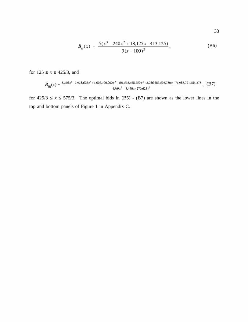
for 425/3 ≤ x ≤ 575/3. The optimal bids in (B5) - (B7) are shown as the lower lines in the

(B7)

top and bottom panels of Figure 1 in Appendix C.

34

Appendix C: Data Figures

Figure 1. Bids (+) in Parts 1 of High-3 (Top Panel) and High-3+, High-3++ (Bottom Panel)Together with Nash Bids (Lower Lines) and Naive Bids (Top Lines)

35

Figure 2. Bids (+) in Parts 1 of High-6 (Top Panel) and High-6+ (Bottom Panel)Together with Nash Bids (Lower Lines) and Naive Bids (Top Lines)

36

Figure 3. Bids (+) in Parts 1 of Low-3 (Top Panel) and Low-3+ (Bottom Panel)Together with Nash Bids (Lower Lines) and Naive Bids (Top Lines)