1

Efficiency and Productivity MeasurementMeasuring Productivity Growth Using

different methods

D.S. Prasada RaoSchool of Economics,

University of Queensland. Australia

2

Measuring Productivity Growth

• Now we consider the case we have data on firms over time – output and input quantities for each firm over t.

• The problem is one of measuring productivity growth – total/multi-factor productivity (TFP/MFP) growth.

• TFP index for two periods s and t would depend upon output and input quantities in the two periods. Let us denote this by F(xt,qt,xs,qs).

• It should satisfy the property:

0,/,,,F allforssss qxqx

In general, the TFP index should be homogeneous of degree +1 q and -1 in x.

3

Four approaches to TFP Measurement

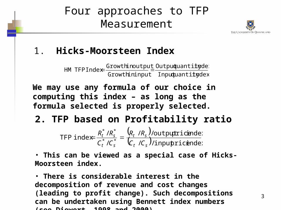
1. Hicks-Moorsteen Index

indexquantityInput

indexquantityOutput

inputinGrowth

outputinGrowthIndexTFPHM

We may use any formula of our choice in computing this index – as long as the formula selected is properly selected.

2. TFP based on Profitability ratio

indexpriceinput//

indexpriceoutput//

/

/indexTFP

**

**

st

st

st

st

CC

RR

CC

RR

• This can be viewed as a special case of Hicks-Moorsteen index.

• There is considerable interest in the decomposition of revenue and cost changes (leading to profit change). Such decompositions can be undertaken using Bennett index numbers (see Diewert, 1998 and 2000).

4

Malmquist Productivity Index

• Malmquist Productivity index makes use of distance functions to measure productivity change.

• It can be defined using input or output orientated distance functions.

• This approach was first proposed in Caves, Christensen and Diewert (1982).

• We just look at the Output-orientated Malquist productivity Index (MPI).

• Using period s-technology:

,

,, ,

,

ss o t t

o s t s t so s s

dm

d

q xq q x x

q x

5

Malmquist Productivity Index

• Using period t-technology:

• Since there are two possible MFP measures, based on period s and period t technology, the MFP is defined as the geometric average of the two:

ss

to

ttt

otsts

to

d

dm

xq

xqxxqq

,

,,,,

0.5

0.5

, , , , , , , , ,

, ,

, ,

s to s t s t o s t s t o s t s t

s to t t o t ts to s s o s s

m m m

d d

d d

q q x x q q x x q q x x

x q x q

x q x q

6

Malmquist Productivity Index - Properties

Properties of Malmquist Productivity Index:

1. It can be decomposed into efficiency change and technical change:

5.0

,

,

,

,

,

,,,,

ssto

ssso

ttto

ttso

ssso

ttto

sstsod

d

d

d

d

dm

qx

qx

qx

qx

qx

qxxxqq

Efficiency change Technical change

2. Malmquist productivity index is the same as the Hicks-Moorsteen index if the technology exhibits global constant returns to scale and inverse homotheticity.

7

Malmquist Productivity Index

x

q

0

E

D

qs

qa

qc

qt

qb

xs xt

Frontier in period s

Frontier in period t

Efficiency change =

as

ct

qq

qq

/

/Technical change =

5.0

/

/

/

/

bs

as

ct

bt

qq

qq

qq

qq

8

Malmquist Productivity Index - Properties

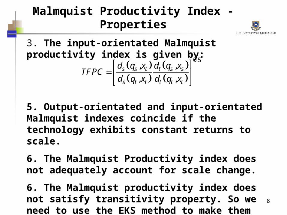
3. The input-orientated Malmquist productivity index is given by:

5. Output-orientated and input-orientated Malmquist indexes coincide if the technology exhibits constant returns to scale.

6. The Malmquist Productivity index does not adequately account for scale change.

6. The Malmquist productivity index does not satisfy transitivity property. So we need to use the EKS method to make them transitive.

0.5, ,

, ,s s t t s s

s t t t t t

d q x d q xTFPC

d q x d q x

9

Malmquist Productivity Index - Properties

7. If panel data on input and output quantities are available then there is no need for price data.

8. If only two data points are available, then we need to use index number approach – may require some behavioural assumptions

10

Productivity Index – components approach

The last approach is to measure productivity change by identifying various sources of productivity growth:

1. Efficiency change2. Technical change3. Scale efficiency change4. Output and input mix effect

Then Productivity change is measured as the product of the four changes above. The resulting index is:

5.0

,

,*

,*

,*

,*,,,

ssto

ttto

ssso

ttso

tststs

d

d

d

dTFPC

qx

qx

qx

qxqqxx

where (*) denotes “cone technology” – the smallest CRS technology that encompasses the technology – in periods t and s.

11

MPI using Index Numbers

• This is the case where we have only two observed points (qt,xt) and (qs,xs).

• In this case we can compute MPI provided we have additional information on prices, (pt,wt) and (ps,ws) and assume that that the firms are technically and allocatively efficient.

• In this case, we have the following result from Caves, Christensen and Diewert which makes it possible to compute the Malmquist productivity index using Tornqvist index numbers.

• The result states that:

12

MPI -Index Number approach

• If the output distance functions in periods s and t are represented by translog functional form with identical second order terms and then under the assumption of technical and allocative efficiency, we can use the Tornqvist output and input quantity index numbers to compute the Malmquist productivity index.

5.0so

too x,x,q,qmx,x,q,qmx,x,q,qm tstststststs

2/*ksK

1k ks

kt

x

x

indexinputTornqvist

indexoutputTornqvist

skistktk 1s1ss *where t and s are the local returns-to-

scale values in periods t and s,

13

MPI -Index Number approach

• If in both periods there is constant returns to scale, then the MPI is simply given by the ratio of the output and input indexes computed using the Tornqvist formula.

• We note that the MPI based on Tornqvist index is not transitive. We can use EKS method to generate transitive Malmquist Productivity indexes.

• Another useful result: If the distance functions are quadratic and under the assumption of technical and allocative efficiency, the Malmquist index is given by the ratio of Fisher output and input quantity index numbers.

1 1

1 1ln ln ln ln

2 2

M K

is it it is js jt jt jsi j

r r q q s s x x

14

Transitive Tornqvist TFP Index

12

1

12

1

12

1

12

1

ln ln ln

ln ln

ln ln

ln ln

Mtransitive

ist it it ii

M

iis is ii

K

jjt jt jj

K

jjs js jj

TFP r r q q

r r q q

s s x x

s s x x

If we apply the EKS method and generate transitive index numbers, we can show that

15

Example

• Recall our example in session 2• Two firms producing t-shirts using labour

and capital (machines)• Let us now assume that they face different

input prices

firm labour capital cost output

x1 w1 x2 w2 q

A 2 80 2 100 360 200

B 4 90 1 120 480 200

16

• In this example we compare productivity across 2 firms (instead of 2 periods)

• First we calculate the input cost shares

• Labour share for firm A

= (280)/(280+2100) = 0.44

• Labour share for firm B

= (490)/(490+1120) = 0.75

• Thus the capital shares are (1-0.44)=0.56 and (1-0.75)=0.25, respectively

17

Ln Output index = ln(200)-ln(200) = 0.0

Ln Input index = [0.5(0.44+0.75)(ln(2)-ln(4)) +0.5(0.56+0.25)(ln(2)-ln(1))]

= -0.13

ln TFP Index = 0.0-(-0.13) = 0.13

TFP Index = exp(0.13)=1.139

ie. firm A is 14% more productive than firm B

18

Malmquist Productivity Index Using DEA

• We recall that the Malmquist productivity index depends upon four different distance functions.

• If we have observed output and input quantity data for a cross-section of firms in periods s and t we can identify the production frontier using DEA and use them in computing the distance needed. In general we need to solve the following four linear programming problems:

0.5

0.5

, , , , , , , , ,

, ,

, ,

s to s t s t o s t s t o s t s t

s to t t o t ts to s s o s s

m m m

d d

d d

q q x x q q x x q q x x

x q x q

x q x q

19

Malmquist Productivity Index Using DEA

• These four LP’s are solved under CRS assumption

[dot(qt, xt)]

-1 = max , , st -qit + Qt 0, xit - Xt 0,

0,

[dos(qs, xs)]

-1 = max , , st -qis + Qs 0, xis – Xs 0,

0,

[dot(qs, xt)]

-1 = max , , st -qis + Qt 0, xis - Xt 0,

0,

[dos(qt, xt)]

-1 = max , , st -qit + Qs 0, xit – Xs 0,

0,

20

Calculation using DEA• TFP growth can be computed using DEA and we need to run 6 different DEA

LPs:

– VRS observation s versus frontier s– VRS observation t versus frontier 1– CRS observation s versus frontier s– CRS observation t versus frontier t– CRS observation s versus frontier t– CRS observation t versus frontier s

• Repeat for each observation between each pair of adjacent periods

• We note here that some VRS LPs may not have a solution – but always guaranteed for CRS

21

Calculation using DEA

Listing of Data File, EG4-DTA.TXT_________________________________

1 22 43 34 55 61 23 44 33 55 51 23 44 33 55 5

_________________________________

Listing of Instruction File, EG4-INS.TXT

___________________________________________________________________ eg4-dta.txt DATA FILE NAME eg4-out.txt OUTPUT FILE NAME 5 NUMBER OF FIRMS 3 NUMBER OF TIME PERIODS 1 NUMBER OF OUTPUTS 1 NUMBER OF INPUTS 1 0=INPUT AND 1=OUTPUT ORIENTATED 0 0=CRS AND 1=VRS 2 0=DEA(MULTI-STAGE), 1=COST-DEA, 2=MALMQUIST-DEA, 3=DEA(1-STAGE), 4=DEA(2-STAGE) ___________________________________________________________________

22

DEAP output

MALMQUIST INDEX SUMMARY OF ANNUAL MEANS year effch techch pech sech tfpch 2 0.844 1.333 0.955 0.883 1.125 3 1.000 1.000 1.000 1.000 1.000 mean 0.918 1.155 0.977 0.940 1.061

MALMQUIST INDEX SUMMARY OF FIRM MEANS firm effch techch pech sech tfpch 1 0.866 1.155 1.000 0.866 1.000 2 1.061 1.155 1.106 0.959 1.225 3 1.000 1.155 1.000 1.000 1.155 4 0.750 1.155 0.806 0.930 0.866 5 0.949 1.155 1.000 0.949 1.095 mean 0.918 1.155 0.977 0.940 1.061 [Note that all Malmquist index averages are geometric means]

23

TFP decomposition with an SFA production function

Suppose we estimate a translog production frontier of the following form using panel data under the standard distributional assumptions

,2

1ln

lnln2

1lnln

2

1

1 110

ititttt

N

nnittn

N

n

N

jnitnitnj

N

nnitnit

uvttxt

xxxβq

i=1,2,...,I , t=1,2,...,T, Efficiency change = TEit/TEis.

where TEit=E(exp(-uit)|eit),

Technical change = ln ln1exp

2is itq q

s t

.

Scale change =

N

nnisnititnitisnis xxSFSF

1)/ln(

2

1exp ,

where isisisSF /)1( ,

N

nnisis

1 and

nis

isnis x

q

ln

ln

.

24

TFP decomposition with an SFA production functionMaximum-Likelihood Estimates of the Stochastic

Frontier Model

Coefficient Estimate Standard Error

t-ratio

0 0.342 0.033 10.230 1 0.453 0.063 7.223 2 0.286 0.062 4.623 3 0.232 0.036 6.391 t 0.015 0.007 2.108 11 -0.509 0.225 -2.263 12 0.613 0.169 3.622 13 0.068 0.144 0.475 1t 0.005 0.024 0.215 22 -0.539 0.264 -2.047 23 -0.159 0.148 -1.073 2t 0.024 0.026 0.942 33 0.021 0.093 0.230 3t -0.034 0.018 -1.893 tt 0.015 0.007 2.176 2

s 0.223 0.025 9.033 0.896 0.033 27.237

Log-likelihood -70.592

25

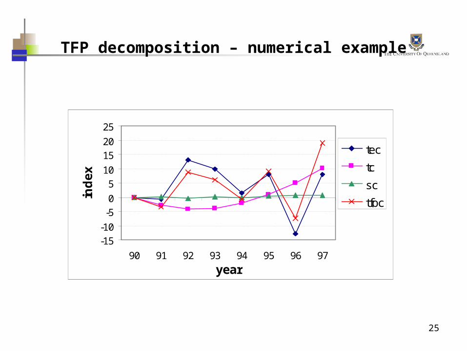
TFP decomposition – numerical example

-15-10

-50

510

1520

25

90 91 92 93 94 95 96 97

year

ind

ex

tec

tc

sc

tfpc