Policy ReseaRch WoRking PaPeR 4324

Efficiency and Equity Impacts of Rural Land Rental Restrictions:

Evidence from India

Klaus DeiningerSongqing Jin

Hari K. Nagarajan

The World BankDevelopment Research GroupSustainable Rural and Urban Development TeamAugust 2007

WPS4324P

ublic

Dis

clos

ure

Aut

horiz

edP

ublic

Dis

clos

ure

Aut

horiz

edP

ublic

Dis

clos

ure

Aut

horiz

edP

ublic

Dis

clos

ure

Aut

horiz

edP

ublic

Dis

clos

ure

Aut

horiz

edP

ublic

Dis

clos

ure

Aut

horiz

edP

ublic

Dis

clos

ure

Aut

horiz

edP

ublic

Dis

clos

ure

Aut

horiz

ed

Produced by the Research Support Team

Abstract

The Policy Research Working Paper Series disseminates the findings of work in progress to encourage the exchange of ideas about development issues. An objective of the series is to get the findings out quickly, even if the presentations are less than fully polished. The papers carry the names of the authors and should be cited accordingly. The findings, interpretations, and conclusions expressed in this paper are entirely those of the authors. They do not necessarily represent the views of the International Bank for Reconstruction and Development/World Bank and its affiliated organizations, or those of the Executive Directors of the World Bank or the governments they represent.

Policy ReseaRch WoRking PaPeR 4324

Recognition of the potentially deleterious implications of inequality in opportunity originating in a skewed asset distribution has spawned considerable interest in land reforms. However, little attention has been devoted to fact that, in the longer term, the measures used to implement land reforms could negatively affect productivity. Use of state level data on rental restrictions, together with a nationally representative survey from

This paper—a product of the Sustainable Rural and Urban Development Team, Development Research Group—is part of a larger effort in the group to assess the impact of land policies on poverty and economic growth. Policy Research Working Papers are also posted on the Web at http://econ.worldbank.org. The author may be contacted at kdeininger@worldbank.org.

India, suggests that, contrary to original intentions, rental restrictions negatively affect productivity and equity. The restrictions reduce the scope for efficiency-enhancing rental transactions that benefit poor producers. Simulations suggest that, by doubling the number of producers with access to land through rental, from about 15 million currently, liberalization of rental markets could have far-reaching impacts.

Efficiency and equity impacts of rural land rental restrictions:

Evidence from India

Klaus Deininger1, Songqing Jin1, and Hari K. Nagarajan2

1 World Bank, Washington DC, USA

2 National Council for Applied Economic Research, New Delhi, India

We would like to thank A. Kaushik, T. Olsen, and S. Vats for excellent research assistance and S. Bery, D. Bradley, R. Buckley, E. Cook, J. Farrington, G. Feder, T. Hanstad, T. Haque, D. Lal, I. Lavadenz, K. Otsuka, S. Rozelle, two anonymous referees, and the editor managing this submission for insightful comments and suggestions. Financial support from the collaborative DFID-World Bank program on land policies and rural development is gratefully acknowledged. The views expressed in this paper are those of the authors and do not necessarily reflect those of the World Bank, NCAER, or DFID.

1. Introduction

Researchers and policy-makers alike have come to realize that unequal access to opportunities arising

from a skewed distribution of assets can be harmful for sustained long-term growth and thus of concern

(Aghion et al. 1999, World Bank 2005). Not surprisingly in view of the important role and long-lasting

impacts of historical land tenure arrangements (Banerjee and Iyer 2005), land reforms have occupied

center stage in India’s policy debates for a long time. Following successful abolition of intermediaries

immediately after independence, award of property rights to sitting tenants through tenancy laws and

expropriation with subsequent transfer of ‘above-ceiling land’ from large land owners to small farmers

were main mechanisms to improve operational and ownership distribution of land. After a slow start,

these policies alone transferred rights to almost 10 mn ha of land, more than three times the land

distributed in land reforms in Japan, Korea, and Taiwan together (King 1977).

Still, despite considerable progress in the past, such legislation has almost ceased to provide new

land access and there is growing concern that, in today’s changed context, maintaining restrictions on

land rental could cause large efficiency losses by precluding efficiency-enhancing transfers of land to

complement rural diversification. Given that, despite increased opportunities for rental, the share of

Indian households participating in rental markets decreased from 26% in 1971 to 11% in 2001 and that in

other countries rental markets have been found to significantly increase productivity (World Bank 2007),

the impact of such restrictions could potentially be very large. This is countered by arguments that rental

markets could, through ‘reverse’ tenancy, give rise to land concentration that is not only inefficient but

would also disempower the poor by forcing them to offer their labor to monopsonistic landlords in local

markets for casual labor that discriminate heavily on the basis of gender and caste.

To assess the functioning of land rental markets and explore efficiency and equity impacts of land

rental restrictions, we use a model of producers who differ in endowments and skills and who face

imperfect labor markets and transaction costs -further increased by policy-induced restrictions- in the land

market. The model would lead us to expect three distinct effects, namely (i) a factor equalization effect

whereby land markets will transfer land to farmers with lower land and higher labor endowments and

with a higher level of ability; (ii) a diversification effect whereby increases in the non-agricultural wage

rate will lead to an increase in land rental activity and a decrease in the equilibrium rental rate; and (iii) a

transaction cost effect whereby higher levels of transaction costs -which may be policy-induced- will

increase the share of producers remaining in autarky thus reducing the number of efficiency-enhancing

land transfers.

1

We use a nationally representative household panel spanning the 1982 to 1999 period to

empirically test these predictions. As land is a state subject, we use cross-state variation in land reform

legislation and its implementation to explore impacts of rental restrictions on land market functioning and

outcomes A panel production function is used to obtain a measure of producers’ ability to assess the

productivity-impact of land rental. Results highlight that, contrary to what is often assumed, land rental

markets help improve productivity and equity by transferring land to more productive and landless or

land-poor households who, in the process, are able to improve their economic status. More importantly,

the pro-poor nature of land markets has improved over time as wealth bias that had characterized such

markets earlier has been eliminated. The fact that land rental is more active in locations with higher levels

of non-farm activity supports the notion that it makes an important contribution to diversification of

income sources in rural areas -in fact, the opportunities opened up through diversification could be a key

factor underlying to help eliminate wealth-related barriers to rental market participation. Our analysis

demonstrates that tenancy restrictions have not only significantly increased the share of producers who

remain in autarky but also prevent land access by more efficient producers. In addition to the results being

very robust, we also find that the magnitudes involved are very large. Simulations suggest that

elimination of these restrictions could prompt an additional 40%-70% of producers to offer land for rental

and, due to the smaller size of land rented in, double the number of those who are able to access land

through rental. Using the mean difference between rental partners to make inferences on potential

productivity impacts suggests that such impacts could be large as well. Thus, while implementing such

laws has helped to obtain social gains in the past, maintaining them is an increasingly potent obstacle to

realizing greater land access by those who are more productive and land-poor or landless and ways to

improve on this may need to be explored.

The paper is structured as follows. Section two describes the history of land reforms and tenancy

regulations in rural India, reviews evidence on the impact of land rental market restrictions and key

differences between rural and urban land markets, and uses this to lay out a conceptual model and

empirical strategy. Section three presents the data used and reviews descriptive statistics for policy

variables and household characteristics. Section four contains econometric results for the production

function and different models of land rental market participation and discusses the results and their

robustness. Section five concludes by putting results into context and drawing out policy implications.

2. Background and conceptual framework

Land reform policy, through abolition of intermediaries, imposition of land ceilings, and regulation of

tenancy contracts, played a key role in India from the moment it started its independent existence. A

review key elements of land rental and ceiling laws, their implementation, and possible links between

2

legislation and land market outcomes is followed by a conceptual model for households’ land market

participation and derivation of hypotheses that can be tested with the data at hand.

2.1 Origins and nature of rural tenancy restrictions in India

Under colonial rule, the main goal of India’s land administration system was to obtain government

revenue. The de facto award of land rights to revenue collectors (zamindars) in large parts of the country

has consequences that affect development to this day (Banerjee and Iyer 2005). Agrarian reform was thus

at the top of the immediate post-independence agenda and the fact that land was put under the

competence of states rather than the Center led to considerable diversity in the timing, substance, and

implementation of reforms across states. Abolition of rent-collecting intermediaries was tackled swiftly

and successfully virtually everywhere. However, ceiling legislation -aiming to legislate a maximum land

holding and force owners to dispose of all that was owned beyond this limit- and tenancy reform -which

had the goal of limiting the rent to be paid for land and prohibiting tenant evictions- took a long time. The

fact that implementation started in earnest only after 1972 allowed landlords to “prepare” by resuming

self cultivation, evicting tenants or transforming them into wage workers, or implement spurious

subdivisions,1 and enthusiasm for such reforms quickly disappeared after 1980 (Appu 1997).

The existence of wide variations in legislation across states provides ample scope to analyze the

impact of such policies on observed outcomes. However, capturing the fine differences in timing,

applicability, modalities of implementation, and definitions inherent in such legislation appears difficult if

not impossible. Rather than trying to do so, we use the share of households who benefited from key

policies as an indicator for policy-induced constraints to the operation of rental markets. Specifically, we

construct for each state the share of households who were awarded tenancy rights and the share of ceiling

surplus area that was actually transferred to beneficiaries.2 As none of the Indian states permit sub-leasing

of lands to which tenants had received permanent rights and most states also impose restrictions on

transfers of land received in the course of implementing ceiling legislation, this is proxies for direct

restrictions on the operation of land rental markets. Both figures also provide an approximation for a state

government’s level of implementation effort, a variable that is exogenous to households’ decisions but

that was shown to be of great importance in earlier studies (Banerjee et al. 2002).

1 Using census figures, Appu (1997) estimates that, to avoid having to give rights to tenants, landlords evicted about 30 mn tenants or about one third of the total agriculturally active population. This is similar to evidence from other countries where landlords often succeeded- to evict tenants in anticipation of legislation to protect tenants against eviction or limit the rents they would have had to pay(Deininger 2003). 2 We use area rather than beneficiaries because in some cases ceiling surplus land was distributed to a collective entity such as a cooperative so that the number of beneficiaries would be misleading. Also, the existence of large discrepancies between the amount of land expropriated and actually distributed -which is due to the fact that in some cases land that had been distributed could not occupied by beneficiaries or was taken back after some time- led us to focus on land actually distributed.

3

Table 1 presents summary statistics by state for total agricultural area and 1980 population

(columns 1 and 2) and our measures of land reform implementation around 1980 (columns 3 and 4).3

Relative emphasis across types of intervention, and the extent of implementation vary across states. More

than 10% of households received tenancy rights in Kerala, Gujarat, West Bengal, and Maharashtra and

more than 5% of area was distributed under ceiling surplus legislation in West Bengal, Andhra,

Maharashtra, Rajasthan, and UP. Some states (e.g. West Bengal, Maharashtra) heavily relied on both

measures, others (e.g. Andhra, Rajasthan and UP) focused exclusively on ceiling surplus, and some (e.g.

Kerala and Gujarat) emphasized tenancy laws. Although -without detailed knowledge on content and

implementation effort- the number of tenancy laws enacted is at best an imperfect proxy for the number

and severity of restrictions on land rental, it is a useful point of reference. We thus include in the mean

number of tenancy laws in each state (column 5) from Besley and Burgess (2000). One notes that the

mean number of laws at any point amounts to 1.5, from none in Haryana to more than 4 in Tamil Nadu.

The correlation between the number of laws and the number of tenants who received rights is low (ρ =

0.28), supporting the notion that legal provisions alone had limited impact and implementation effort was

required.

While we do not separate it out in the table, a more detailed look at the time dimension of these

measures allows a number of conclusions (Kaushik 2005). First, land reform has been a major effort; up

to 2000, land reform laws resulted in the transfer of almost 10 mn ha, 2.5 mn ha under programs to

redistribute of ceiling surplus land and 7.35 mn ha under tenancy legislation.4 Second, after a spurt of

land transfers in the 1970s and 1980s, progress has slowed down considerably; in fact between 1995/96

and 2003/04, i.e. for almost a decade, progress in awarding land rights to tenants had come to a complete

standstill.5

2.2 Tenancy legislation and rent controls: International evidence

Even though empirical evidence on the impact of rent ceilings and other forms of tenancy control in rural

areas is limited, the issue has been analyzed in urban contexts where rent control is a textbook example

for policies that can be effective to transfer resources in the short term but will be associated with

inefficiencies in the medium to long run (Arnott 2003). The key reason, which also formed the basis for

analytical approaches, is that, by fixing rents below their equilibrium level, controls reduce the supply of

3 Wherever available, the level of the respective variables in 1980 and 1998, respectively, is used as a right hand side variable in the regressions. 4 The amount of land involved is much larger than what was redistributed in other Asian land reforms such as Japan (2 mn has), Korea (0.58 mn has) and Taiwan (0.24 mn has). In terms of total area distributed, this puts India on par with Mexico which, in a much more land-abundant setting, and starting in 1917, managed to distribute slightly more than 13 mn ha (Deininger 2003). 5 The increment in ceiling surplus land transferred during the period amounted to only 10,800 ha which is only about one tenth of the land declared ceiling surplus which had not been distributed. The fact that all the remainder remains tied up in litigation suggests that further progress in achieving redistribution of ceiling land could be slow -it would take almost 90 years to dispose of remaining ceiling surplus cases if the current pace is maintained- and that, by clogging up the court system and preventing it from quickly dispensing justice in other urgent matters, the ceiling legislation may impose external effects beyond land rental markets (Moog 1997).

4

new housing or maintenance of existing units by landlords who face an artificially reduced price

(Gyourko and Linneman 1990). Thus, although they transfer resources from landlords to sitting tenants at

the time of imposition, they make access to rental property more difficult thereafter (Basu and Emerson

2000). With a constant or decreasing number of beneficiaries and an increasing number of new entrants

who need to access to land in distorted markets, social cost of maintaining land rental restrictions will

increase over time (Glaeser 2002). While rent controls may be useful to deal with emergencies in the

short term, other policies may be more effective (Malpezzi and Ball 1991), have fewer undesirable side-

effects including reduced tenant mobility (Munch and Svarer 2002), and can be better targeted.

While there is little empirical evidence on the impact of rental restrictions in rural areas, a number

of reasons would lead one to expect that it will go far beyond the price effects on which the urban

literature has focused. First, due to labor market imperfections, the way in which rural land is used will

have a clear impact on productive efficiency (Binswanger et al. 1995). Second, supply of housing to

urban markets will be less elastic as owners can not revert to own- or wage labor-based cultivation, an

issue that has been highly relevant in India (Appu 1997). Third, as rural rents are generally defined as an

in-kind output share, contract terms will be less flexible than urban ones, limiting the scope for

circumventing them by adjusting rental rates (Basu and Emerson 2003). Finally, rights given to tenants

are heritable but non-transferable and still require rent payment to the landlord, thus reducing both

parties’ incentives for land-related investments and the scope to increase allocative efficiency through

sub-leasing.6

While all of these issues could significantly add to the long-term cost of land reforms, they have

not featured prominently in the large literature on Indian land reforms (Warriner 1969, Thorner 1976,

Besley and Burgess 2000, Banerjee et al. 2002). Exploring this by assessing how land rental markets

work and to what extent they are affected by tenancy restrictions will allow us to get an indication of such

cost and help put the policy debate on land markets in India on a more robust empirical footing.

2.3 Conceptual framework

A key rationale for producers to engage in land markets is the desire to adjust for differences in their

existing endowments of land and family labor. Following similar models in the literature (Carter and Yao

2002), let household i be endowed with fixed amounts of labor ( iL ) and land ( iA ), and a given level of

agricultural ability ( iα ). Agricultural production follows a production function f(αi,,li,a,Ai) with standard

6 The tenant will be unlikely to invest as doing so will result in an immediate increase of the rent whereas investment by the landlord is unlikely as part of the benefits will go to the tenant.

5

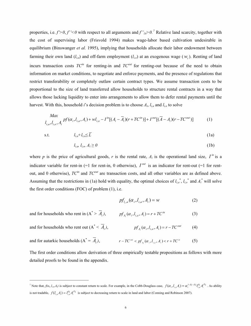
properties, i.e. f’>0, f’’<0 with respect to all arguments and f’’lA>0.7 Relative land scarcity, together with

the cost of supervising labor (Frisvold 1994) makes wage-labor based cultivation undesirable in

equilibrium (Binswanger et al. 1995), implying that households allocate their labor endowment between

farming their own land (li,a) and off-farm employment (li,o) at an exogenous wage ( ). Renting of land

incurs transaction costs TC

iwin for renting-in and TCout for renting-out because of the need to obtain

information on market conditions, to negotiate and enforce payments, and the presence of regulations that

restrict transferability or completely outlaw certain contract types. We assume transaction costs to be

proportional to the size of land transferred allow households to structure rental contracts in a way that

allows those lacking liquidity to enter into arrangements to allow them to defer rental payments until the

harvest. With this, household i’s decision problem is to choose Ai, li,a and li,o to solve

)])([()])([(),,(,, ,,

,,

outi

outinii

inoiiaii

ioiaiTCrAAITCrAAIwlAlpf

AllMax

−−++−−+α (1)

s.t. li,a+li,o≤ L (1a)

li,a, li,o, Ai ≥ 0 (1b)

where p is the price of agricultural goods, r is the rental rate, Ai is the operational land size, inI is a

indicator variable for rent-in (=1 for rent-in, 0 otherwise), outI is an indicator for rent-out (=1 for rent-

out, and 0 otherwise), TCin and TCout are transaction costs, and all other variables are as defined above.

Assuming that the restrictions in (1a) hold with equality, the optimal choices of li,a*, li,o

* and Ai* will solve

the first order conditions (FOC) of problem (1), i.e.

wAlpf iaiiali=),,( ,, α (2)

and for households who rent in (A* > iA ), (3) iniaiiA TCrAlpf

i+=),,( ,α

and for households who rent out (A* < iA ), (4) outiaiiA TCrAlpf

i−=),,( ,α

and for autarkic households (A* = iA ), (5) iniaiiiA

out TCrAlpfTCr +<<− ),,( ,α

The first order conditions allow derivation of three empirically testable propositions as follows with more

detailed proofs to be found in the appendix.

7 Note that, f(αi,,li,a,Ai) is subject to constant return to scale. For example, in the Cobb-Douglass case, . As ability

is not tradable, is subject to decreasing return to scale in land and labor (Conning and Robinson 2007).

21,

211, ),( ββββαα iaiiiaii AlAlf −−=

21,, )( ββ

iaiiai AlAlf =

6

Proposition 1: The amount of land rented in (out) is strictly increasing (decreasing) in

households’ agricultural ability, αi, and strictly decreasing (increasing) in the land endowment iA . Land

rental will transfer land to efficient, but land-poor producers, thereby contributing to higher levels of

productivity and more efficient factor use in the economy. For households renting in or out land, this

proposition can be derived by totally differentiating both sides of equations (2) and (3) or (2) and (4) with

respect to αi or iA . Manipulating terms yields ∂Ai*/∂αi >0 (or ∂Ai

*/∂ A <0). Since aiin or ai

out, the amount

rented in or rented out, respectively is defined as either Ai*- iA or iA -Ai

*, the result for aiin and ai

out

follows.

Proposition 2: The presence of transaction costs defines two critical ability levels αl(TCout, ..) and

αu(TCin, ..) such that households with ability αi∈[αl, αu] will remain in autarky. Any increase in TCin or

TCout will expand the autarky range, thus reducing the number of producers participating in rental markets

and the number of efficiency-enhancing land transactions. Compared to a situation with no transaction

cost, this will decrease productivity and social welfare. To see this, note that the cutoff points αl and αu

can be obtained from (4) and (3) by setting Ai*= iA and li,a= where is autarkic household i’s

optimal amount of labor in agricultural production which can be derived from (2) at A

*,ail

*,ail

i*= iA . Defining

, we can solve for α21,

211, ),,( ββββαα iaiiaii AlAlf −−= l and αu explicitly as

2111

121*,2 )(

ββ

βββα

−−

− ⎟⎟⎠

⎞⎜⎜⎝

⎛ −=

AlTCr

ai

out

l and

2111

121*,2 )(

ββ

βββα

−−

− ⎟⎟⎠

⎞⎜⎜⎝

⎛ +=

AlTCr

ai

in

u . Differentiation of αl or αu with respect to the corresponding transaction cost

variable TCout or TCin then yields the result of interest.

Proposition 3: Increases of the exogenously given wage for off-farm employment will imply that

higher amounts of land are transacted in rental markets as households with low agricultural ability who

join the off-farm labor market will supply more land. This leads to a decrease in the equilibrium rental

rate which will prompt high-ability workers (specializing in agricultural production) to rent in more land.

To derive this proposition, assume without loss of generality that the economy contains n

households who are endowed with identical amounts of land and labor A and L but different levels of

farming ability αi and that the latter is uniformly distributed between α and α . We also assume that, with

fixed setup costs, households give up agricultural production completely and rent out all their land if the

amount of labor to be allocated optimally to agricultural production is less than lac. To be able to derive a

closed form solution, we abstract from transaction costs (i.e. letting TCin=TCout=0) and use an explicit

7

functional form . With an exogenous wage w and prices normalized to 1, the

rental rate r will be determined endogenously and first order conditions (dropping i for notational clarity)

simplify to

21,

211, ),,( ββββαα iaiiaii AlAlf −−=

(6) wlAf aal== −−− )1(

2)1(' 2121 ββββ βα

and (7). rlAf aA == −−− 2121 )1(1

)1(' ββββ βα

As A* is proportional to households’ farming ability α, the market clearing condition can be expressed as

∫ =α

αα AndA* , which together with (6) and (7) can be used to solve for A*, la

*and r* as

)(2

22

*

ααα

−=

AnA , )

211

(

2

)12

1(

)12

1(

22*

2ββ

ββ

βααα−−

−

⎟⎟⎠

⎞⎜⎜⎝

⎛ −= w

Anla and 1

)21

1(

2

)12

1(

)12

121(

22*

2ββ

αα ββ

βββ

−−

−−+

⎟⎟⎠

⎞⎜⎜⎝

⎛ −= w

Anr

Setting la*=la

c allows to solve for the critical level of ability αc below which households will rent out all

their land endowment. For households who continue farm production, we solve for the new optimal

operational land size (A**) and new rental rate (r**) based on (6), (7) and the new market clearing

condition ( ∫ =α

αα

cAndA ** ). Setting AA =** allows us to solve for the farming ability by household who

remain autarkic αau. Taking derivatives of αc, A**, αau and r** with respect to w yields: ∂αc/∂w>0,

∂A**/∂w>0, ∂αau/∂w<0 and ∂r**/∂w<0, suggesting that, as off-farm opportunities increase, a larger

number of households will drop farm production and rent out all their endowment, the equilibrium rental

rate will decrease, households who remain in agricultural production cultivate more land, and a greater

number of households will rent in land.

2.4 Estimation strategy

Equations (2)-(5) indicate that producers’ decision to enter land rental markets depends on their marginal

productivity in autarky, MP( A ) as compared to the rental rate to be paid rin(T) or received rout(T) which

is a function of transaction costs. Formally, the three regimes are characterized by

⎪⎭

⎪⎬

⎫

>+<<+<=

<+>

)r(TC ε) AMP()r(TC ) A MP() r(TC

)r(TC ε) AMP(

ini

ini

out

outi

:)Aregime(Ain -Rent III.:)A(A regimeAutarky II.

:)A(A regimeout -Rent I.

i*i

i*i

i*i

(8)

A producer’s marginal product MP( A ), will depend on his or her ability (α), endowment with land ( A ),

family labor ( L ), assets (K), and the opportunity cost of labor which will be affected by the level of

education (E) and the presence of opportunities in the local off-farm labor market (O). Defining a well-

8

behaved net earning function g(α, A , L ,K,E,O) with first derivative g’(.),we can write a linear version of

the latter as MP( A )=g’(α, A , L ,K,E,O)= β0 + β1α + β2 A + β3 L + β4K + β5E + β6O. Transaction

costs are expected to depend on policy variables S, household characteristics Z, and a time dummy D99.

Defining an index variable yi such that yi = 1 if A*< A ; yi = 2 if A*= A ; yi = 3 if A*> A , we can

rewrite (8) as an ordered probit model that can be estimated using maximum likelihood methods.

)9(

3Pr

2Pr1Pr

654321099

3210

654321099

3210

654321099

3210

654321099

3210

⎪⎪⎭

⎪⎪⎬

⎫

−−−−−−−+++>Φ==−−−−−−−+++<

<−−−−−−−+++Φ==−−−−−−−+++<Φ==

O}EKLADZS{ε)ob(yO}EKLADZS

OEKLADZS{ ) ob(yO}EKLADZS{ ) ob(y

iii

ii

ii

βββββαββδδδδβββββαββδδδδ

εβββββαββηηηηβββββαββηηηηε

Variables we expect to affect marginal productivity are agricultural ability (α), the derivation of

which will be discussed below, a dummy for landlessness and the log of the land endowment to represent

A , the number of members in the 14-60 and below 14-year age group to represent L , the value of assets

and the share of agricultural assets (livestock, implements, and agricultural structures) for K, the head’s

age (as a proxy for experience) and a dummy for primary education to represent human capital E, and

mean village income O to represent wage labor opportunities in off-farm labor markets. Transaction cost

of land rental participation are affected by producer’s caste status, (Z), a time dummy (D99), and land

policy (S) which is proxied by either the share of households who were recognized under tenancy reform,

the share of area distributed under ceiling legislation, or the number of tenancy laws enacted as discussed

earlier.

The propositions from our model allow making predictions on the signs of individual coefficients.

The factor equalization from proposition 1 implies that rental markets will transfer land to more

productive producers (β1>0) with lower levels of land endowments (β2<0) and more family labor (β3>0).

The hypothesis of wealth bias in rental markets, possibly due to credit market imperfections, translates

into β4>0. Diversification effects implied by proposition 3 suggest that producers with higher levels of

education have better off farm opportunities and will be less likely to rent in land (β5<0) and that higher

levels of non-agricultural wages, proxied by O, will make renting in less likely (β6<0).

Proposition 2 implies that, by moving the cut-off points where producers shift from renting out to

autarky and from autarky to renting in, respectively, rental market restrictions expand the range of autarky

but do not affect producers’ marginal product.8 We thus expect η1>0 and δ1<0, respectively. By the same

logic, higher transaction costs for producers from scheduled and backward castes imply η2>0, and δ2<0

8 It is intuitive that rental restrictions will directly affect whether or not households participate but, unless there are selectivity issue, are unlikely to affect producers’ marginal productivity. Indeed testing for selectivity of rental market participation, by including rental restrictions in the marginal product equation as well, does not produce conclusive results.

9

while a reduction over time in transaction costs due to better access to information implies η3<0 and

δ3>0.

A key element of the regression (8) is households’ agricultural ability α. As the data available are

a panel of households and their offspring who were observed in 1982 and again in 1999, we can recover

this parameter from a panel production function using household (or dynasty) fixed effects to proxy for

ability (Deininger and Jin 2007). Let technology be represented by the Cobb-Douglas production function

)exp()exp( 4321 tXKLAQ ijtijtijtijtjiijt φαα θθθθ+= (10)

where Qijt is the value of agricultural output produced by household i in village j in year t; Aijt, Lijt and Kijt,

Xijt are total cultivated area, labor for crop production, value of agricultural assets, and amounts of

chemical fertilizer, organic manure, pesticides, and seeds, θ1, θ2, θ3, and θ4 are technical coefficients, αj is

a time invariant village level parameter reflecting, among others, access to markets, infrastructure, and

other time invariant factors such as climate, αi is the time invariant household fixed effect which we use

to measure of ability, and t is a time dummy so that exp(φt) measures productivity changes over time. To

estimate this, we let αij = αi +αj, take logarithms of both sides, and add an iid error term to obtain

qijt = αij +θ1aijt + θ2 lijt + θ3 kijt + θ4 xijt + φt + εijt (11)

where lower case letters are logarithms. With multiple observations per household, we can subtract means

qijt - ijq = αij - jiα + θ (Zijt - ijZ ) + φ (t- t ) + εijt - jiε (12)

where Zijt is a vector including a, l, k, x with coefficients θ . As αij - jiα = 0, this can be simplified to

qijt - ijq = θ (Zijt - ijZ ) + φ (t- t ) + εijt - jiε (13)

This can be used to obtain , composed of a producer’s idiosyncratic ability αijα̂ i and unobserved

village attributes αj. Letting the latter be the average of household fixed effect in the village

(Mundlak 1961) allows to obtain ∑=i

jijj n/)ˆ(ˆ αα iα̂ , the producer-specific effect by subtracting jα̂ from

ijα̂ .9

3. Data sources and descriptive evidence

9 An alternative approach is to use a stochastic frontier production function to determine producers’ level of technical efficiency in each of the periods. This assumes that the disturbance term is composed of two additive components vi and ui where vi is pure white noise and ui~N+(0, δu

2) captures producers’ level of technical inefficiency TEi = exp(-ui) (Coelli 1995). While the strong distributional assumption and the fact that ui captures other shocks imply that this is inferior to the panel approach, the fact that a large number of households dropped out of the panel makes this an attractive alternative which we use as a robustness check for our results below.

10

Before discussing the econometric results, we describe the data by presenting evidence on socio-

economic characteristics as well as land market participation and changes in these variables over time.

This allows us to explore changes of the economic structure, growth, and asset accumulation by

individuals and at the village level. Concerning rental markets, our interest is to find out whether our

hypotheses are supported by descriptive evidence or whether, possibly as a result of “reverse tenancy”

rental markets lead to transfers from small to larger producers rather than to land-poor ones.

3.1 Household characteristics

The data used in the analysis come from two rounds of NCAER’s ARIS/REDS survey conducted in 1982

and 1999, respectively. This survey, the first rounds of which were implemented in 1968-71 to evaluate

the impact of an agricultural development program, covers all of India’s major states. Even though the

first round sample, stratified by farm size and wealth class, was limited to project areas, the survey was

expanded in 1982 to make it more representative at the national level, covering slightly less than 5,000

households (Foster and Rosenzweig 1996). The 1999 sample contains the 1982 sample and replacements

for those no longer present. If the original household had split, all of the households belonging to the

same dynasty in the original village plus a sub-sample of successor households outside the village were

interviewed, bringing the total to about 7,500 households (Foster and Rosenzweig 2004).

Table 2 reports descriptive statistics for the whole country and its four main regions in both

periods.10 We note that there has been a marked increase in educational attainment, as illustrated by the

fact that the share of household heads with primary schooling completed increased from about 26% in

1982 to 50% in 1999. The gap that had earlier separated Northern and Southern states also narrowed

considerably. At the same time, population growth led to a decline in the average land endowment, from

3.3 ha in 1982 to 2.1 ha in 1999, and a small increase in landlessness, from 22% to 24%. Average

household size decreased, from 6.9 to 6.0, with about 4 in the 14 to 60 age category, 0.4 aged above 60,

and 2.4 as compared to 1.8 below the age of 14. The share of female headed households is, with 6.8%,

almost the same in both periods, although female headship is more pronounced in the South than in other

regions.

Survey results also point towards an annual increase of per capita income of 3.1% during the

period under concern. This aggregate masks pronounced differences across regions with the South having

caught up and even replaced the North as the region with the highest income in the second period. Use of

the information from the listing exercise allows us to compute the Gini coefficient for self-assessed

income in a way that includes all households in the sampled villages. With a Gini coefficient of 0.32 in 10 We group states into four regions as follows: The North includes the states of Haryana, Himachal Pradesh, Punjab, and Uttar Pradesh; the West includes Gujarat, Maharashtra, Madhya Pradesh, and Rajasthan; the East includes Assam, Bihar, Orissa, and West Bengal; and the South includes Andhra Pradesh, Karnataka, Kerala, and Tamil Nadu.

11

the first and 0.31 in the second period, inequalities in income remain modest and have not appreciably

increased between the two periods. The overall improvement in living standards as illustrated by

increased income is mirrored by a significant rise in asset values of approximately 6% per year.11 It is

worth noting that, with a Gini coefficient of 0.60 in 1982, inequality in assets is higher than income

inequality, as found in other parts in the world as well. However, this coefficient has actually decreased to

0.56 in the second period. While overall asset endowments have increased, the broad composition of

households’ asset portfolio shows greater stability; the house and consumption durables make up the

largest share in both periods (57.5% and 56.9%, respectively in 1982 and 1999), followed by financial

and off-farm assets (26.7% and 23.2%), and farm assets including livestock (15.8% and 19.9%).

The bottom panel illustrates the diversification of income sources achieved during the period by

highlighting the share of households who participated in various activities, noting that households

generally rely on more than just one income source. Three observations are of particular interest. First,

despite a drop by about 7 and 15 percentage points in the share of households engaging in crop and

livestock production, respectively (from 70% to 63% for crop and from 78% to 63% for livestock), self

employment in agriculture remains the most important source of employment in India’s rural economy.

The fact that this is followed by agricultural wage employment, the share of which has actually increased

over the period (from 37.6% to 43.3%) points to a continued importance of agriculture and the importance

of agricultural wage employment for the landless. A second finding of interest is that the share of

households engaging in self-employment in rural India has been more or less constant, implying that

growth of the rural non-farm sector has been just large enough to absorb population growth. This

contrasts with other countries where the rural non-farm economy developed as a result of out-migration of

labor or due to households taking up non-farm self employment. In fact, according to our data, the main

source of income diversification was growth of non-farm wage employment, participation in which

increased from 8.6% in 1982 to 20% in 1999. This fact, which has also been observed elsewhere (Foster

and Rosenzweig 2004), could result from the government’s emphasis on creating rural employment

through mechanisms ranging from direct subsidies for firms to set up in remote areas to industrial and

labor market regulation such as small scale reservation acts (Besley and Burgess 2004).

3.2 Operation of land rental markets

To provide evidence on the extent to which our hypotheses on land markets are borne out descriptively,

Table 3 presents key variables by households’ land rental participation status (rent in, rent out, or

autarky). It points towards a large increase in the level of land market activity over the period; from 5.3%

11 While part of this increase may be due to improvements in the survey instrument that resulted in better measurement of assets in the second period, it is impossible to test this hypothesis as disaggregated data for 1982 were not available.

12

and 2% for renting out and renting in, respectively, in 1982, the share of market participants has increased

to 10.7% and 4.1%, in 1999.12 Descriptive figures also support the propositions from our model and the

notion of better rental market functioning in the second, as compared to the first period.

Comparing the per capita land endowment for land owners who either remained in autarky (0.51

ha and 0.36 ha in 1982 and 1999, respectively), rented in (0.28 ha and 0.20 ha), or rented out (0.68 ha and

0.64 ha) in the two periods illustrates that, in both periods, rental provided opportunities for relatively

land-scarce and labor-abundant households to gain access to land. Land markets transferred land from

households with more educated and female heads to male headed ones with lower educational attainment.

We also note that the share of landless who had gained access to land through rental markets increased

from 12% in the first to 37% in the second period, suggesting a marked expansion of outreach towards

this group over time. Noting that our sample represents about 130 mn rural households, in 1999 about 15

mn households -a quarter of them landless- were able to use markets as a means to get access to land.

This figure is not only much larger than the number of those who got access to land through land reform

but also that, given the magnitudes involved, even policies with “modest” impact on the functioning of

land rental markets could have implications for a large number of households.

Comparing levels of consumption and assets for households who differ in the nature of their land

market participation reinforces the notion that rental provides opportunities for poor segments of the

population to access productive resources and thereby improve their well-being, especially in the second

period. The value of all assets owned by rent-in households in 1999 is, with Rs. 33,839, more than 25%

below the average, compared to asset ownership that is similar to the mean for autarkic households and

about 33% higher than the mean for those renting out, supporting the notion that it is the asset-poor who

benefit from the access to land which rental markets provide. The narrowing of the gap between rent-in

and average households with respect to per capita expenditure supports the hypothesis of land markets

making a positive contribution to the livelihood of participants. Finding significant differences in the

composition of the asset portfolio between rent-in and rent-out households, with the former having

relatively more of their wealth in farming and livestock and the latter in off-farm and financial assets is

not too surprising.

While higher participation in crop and livestock production by those renting in should not come

as a surprise, the high share of renters engaging in (agricultural) wage employment suggests that land

rental provides wage laborers with opportunities to earn additional income. At the same time, the fact that

12 While this is a large change, the level of rental market activity increased more rapidly, and in a shorter period, in other Asian countries such as China or Vietnam, despite the fact that the more egalitarian land ownership distribution in these countries would put greater limits on the potential of land markets to equalize operational holdings than in India. In Vietnam, the share of households renting in increased form 3.8% to 15.8% in the 5-year period between 1993 and 1998 (Deininger and Jin 2007). In China, the same figure increased from 2.3% in 1996 to 9.4 in 2001 (Deininger and Jin 2005).

13

-in contrast to what was found in 1982- non-farm self employment is much higher among rent-in

households than either the mean or those who remained in autarky suggests that land rental is not an

obstacle to participation in the rural non-farm economy. To the contrary, renting may provide an

opportunity to accumulate experience and capital to replace the “agricultural ladder” (Spillman 1919)

with a general increase in occupational mobility including the non-farm sector (Alston and Ferrie 2005).

4. Econometric evidence

We find that measures to implement land reform, whether proxied by the number of laws passed, the area

transferred under ceiling legislation, or the number of beneficiaries from tenancy acts, constrain rental

market activity, thereby reducing both equity and efficiency. They make it more difficult for producers

with high ability, including the landless, to gain access to land while at the same time constituting an

obstacle for giving up farming by those with low ability who want to get out of agriculture.

4.1 Production function

To obtain a measure of households’ or dynasties’ agricultural ability, a production function, coefficients

for which are reported in Table 4, was estimated. Although a significant number of households for whom

production is observed only in one of the periods are dropped, the specification fit the data very well with

an R2 of 0.76 for the fixed effect estimation, and of 0.83 for OLS with coefficient estimates from both

being close to each other. Concerning the individual variables, land is estimated to be by far the most

important input to crop production; doubling cultivated land area alone would lead to a 50% to 58%

increase in total crop production. This is followed by seed expenditures and labor use with an estimated

elasticity of 13% to 17% each. Compared to these, returns to fertilizer, pesticides, irrigation and assets are

more moderate with elasticities of about 5%, 2-3%, 1-2%, and 4% for expenditure on fertilizer, pesticides,

irrigation and others. While neither education nor the gender of the household head are significant, land

quality matters and doubling land values, which we use as a proxy for land quality, would increase total

output by 11-12%. Significant variation of ability across households could imply that, even without a

strong pull from non-agricultural employment opportunities, the scope for market-mediated transfers to

bring about efficiency gains could be large. The estimated size of technological change between the two

periods is between 14 and 24%.13

4.2 Determinants of land market participation

13 The fact that coefficients for the frontier production function are very similar to those obtained using OLS and the panel increases our confidence in the robustness of the results.

14

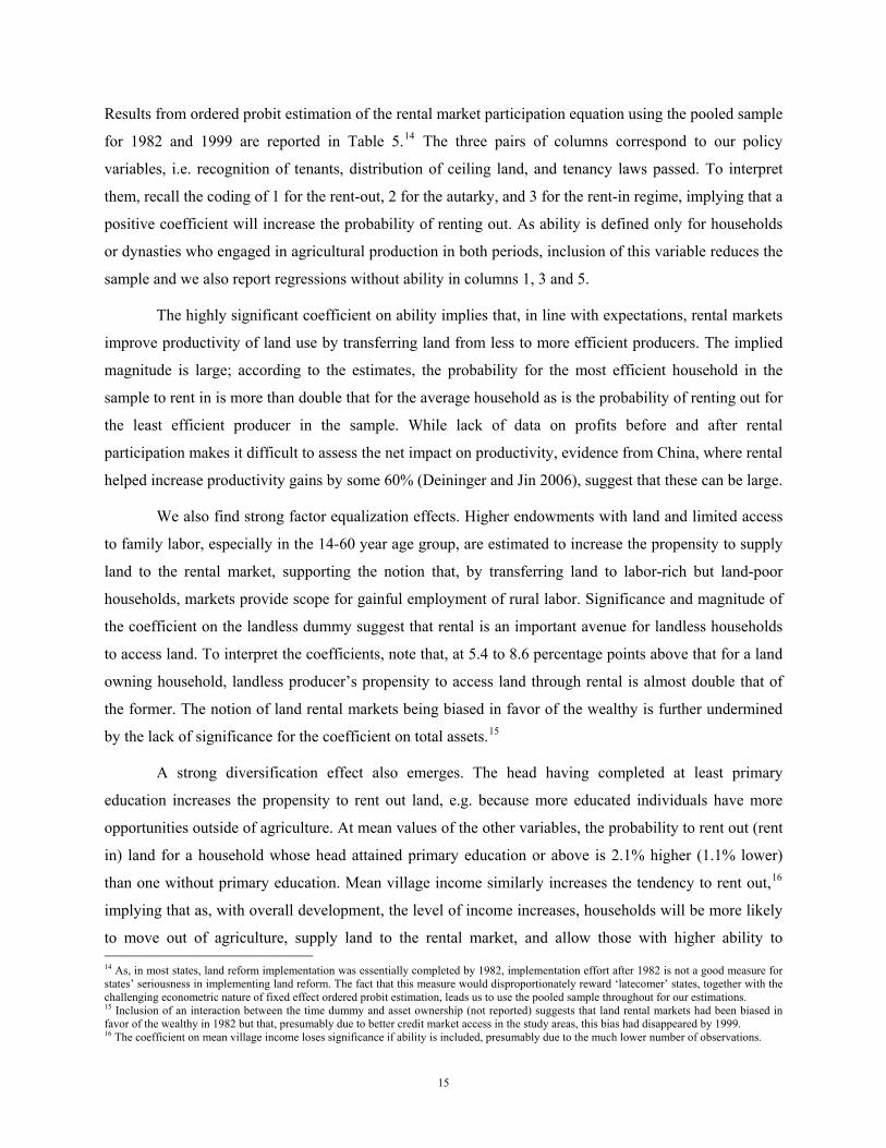
Results from ordered probit estimation of the rental market participation equation using the pooled sample

for 1982 and 1999 are reported in Table 5.14 The three pairs of columns correspond to our policy

variables, i.e. recognition of tenants, distribution of ceiling land, and tenancy laws passed. To interpret

them, recall the coding of 1 for the rent-out, 2 for the autarky, and 3 for the rent-in regime, implying that a

positive coefficient will increase the probability of renting out. As ability is defined only for households

or dynasties who engaged in agricultural production in both periods, inclusion of this variable reduces the

sample and we also report regressions without ability in columns 1, 3 and 5.

The highly significant coefficient on ability implies that, in line with expectations, rental markets

improve productivity of land use by transferring land from less to more efficient producers. The implied

magnitude is large; according to the estimates, the probability for the most efficient household in the

sample to rent in is more than double that for the average household as is the probability of renting out for

the least efficient producer in the sample. While lack of data on profits before and after rental

participation makes it difficult to assess the net impact on productivity, evidence from China, where rental

helped increase productivity gains by some 60% (Deininger and Jin 2006), suggest that these can be large.

We also find strong factor equalization effects. Higher endowments with land and limited access

to family labor, especially in the 14-60 year age group, are estimated to increase the propensity to supply

land to the rental market, supporting the notion that, by transferring land to labor-rich but land-poor

households, markets provide scope for gainful employment of rural labor. Significance and magnitude of

the coefficient on the landless dummy suggest that rental is an important avenue for landless households

to access land. To interpret the coefficients, note that, at 5.4 to 8.6 percentage points above that for a land

owning household, landless producer’s propensity to access land through rental is almost double that of

the former. The notion of land rental markets being biased in favor of the wealthy is further undermined

by the lack of significance for the coefficient on total assets.15

A strong diversification effect also emerges. The head having completed at least primary

education increases the propensity to rent out land, e.g. because more educated individuals have more

opportunities outside of agriculture. At mean values of the other variables, the probability to rent out (rent

in) land for a household whose head attained primary education or above is 2.1% higher (1.1% lower)

than one without primary education. Mean village income similarly increases the tendency to rent out,16

implying that as, with overall development, the level of income increases, households will be more likely

to move out of agriculture, supply land to the rental market, and allow those with higher ability to 14 As, in most states, land reform implementation was essentially completed by 1982, implementation effort after 1982 is not a good measure for states’ seriousness in implementing land reform. The fact that this measure would disproportionately reward ‘latecomer’ states, together with the challenging econometric nature of fixed effect ordered probit estimation, leads us to use the pooled sample throughout for our estimations. 15 Inclusion of an interaction between the time dummy and asset ownership (not reported) suggests that land rental markets had been biased in favor of the wealthy in 1982 but that, presumably due to better credit market access in the study areas, this bias had disappeared by 1999. 16 The coefficient on mean village income loses significance if ability is included, presumably due to the much lower number of observations.

15

increase their holdings and income levels. This phenomenon, which has also been observed in China,

highlights the importance of rental markets with economic development and suggests that imposing

restrictions on the operation of such markets could not only inflict efficiency losses but also become more

difficult over time.

Regarding the lower bound equation, regressions suggest that policy restrictions will lead to a

significant and quantitatively large reduction of land supply to rental markets. Estimated effects are

weakest for the number of laws (columns 5 and 6) and strongest for recognition of tenants (col. 1 and 2),

consistent with the notion that implementation is more important than mere legislation and that landlords

will be less willing to rent out if doing so can attenuate their property rights or if there are limits on their

ability to negotiate the amount of rent.17 The share of land affected by redistribution of ceiling land is in

the middle between these two, consistent with expectations that ceiling legislation poses less of a threat

than tenancy regulation -as the latter applies to all market participants irrespective of their holding size-

and enforcing it is more politically controversial and administratively complex than implementing

tenancy legislation. Coefficients on other variables suggest that, even after adjusting for policies,

scheduled and backward castes are less likely to rent out land than the remainder of the population,

possibly due to lower levels of social capital and less opportunity to find partners in rental markets or to

enforce protection of property rights for rented land. The highly significant and positive coefficient on the

1999 dummy illustrates that, over time, land rental supply increased significantly, possibly due to

information access. To quantify the impact of policy restrictions we compute, for every household, the

predicted probability to rent out with actual values for all right hand side variables and with the tenancy

restriction variable taking a value of zero. Taking the difference between these two values as a measure

for the impact of tenancy restrictions suggests that their removal could lead to a considerable increase in

renting out, by between 40% and 70%.

Turning to the (upper) bound between autarky and renting in, the positive coefficient on all the

policy variables suggests that over and above the reduction in supply they also depressed demand, making

it more difficult for households to obtain land through rental. Across policy variables, those relating to the

intensity of enforcement are again more significant; in fact the number of laws, while of the expected

sign, is not different from zero at conventional levels. In most equations, coefficients are bigger for the

upper as compared to the lower bound, suggesting that the impact of policy-induced restrictions will be

larger on the demand side. Applying the methodology used earlier for the lower bound to assess predicted

impacts of eliminating policy restrictions suggests that, with a coefficient much larger than for the upper

bound, removal of tenancy restriction could double participation rates by rent-in households.

17 Note that the coefficients on the number of laws and the amount of land distributed via ceiling laws lose significance in the smaller sample.

16

Consistent with what emerged for the upper bound, we also find that backward and scheduled

castes are more likely to remain in autarky and that over time, the size of the autarky area has decreased,

i.e. land rental markets have become more active. While this is encouraging sign and suggests that time

may partly offset undesirable impacts of rental regulation, the magnitude of the coefficients is small;

estimated coefficients imply that almost a century will be required to fully offset these effects. Together

with case studies suggesting that circumventing such legislation is easier for the rich than for the poor

(Yugandhar 1996, Thangaraj 2004), this implies that passage of time is unlikely to eliminate the negative

effects of tenancy regulation or do so in an equitable manner. To test the robustness of our conclusions,

we compare results those derived from using the productivity measure derived from the frontier

production function instead of the panel. Doing so increases the sample size by two thirds but leads to

very similar substantive conclusions; in particular providing strong support to the factor equalization and

diversification effects as well as the negative impact of policy restrictions (Appendix Table 1).

4.3 Efficiency impact of land rental restrictions

Results thus far highlight that policy restrictions negatively affected efficiency by reducing overall rental

market and impeding access to land by the poor. Interacting policy variables with producers’ estimated

productive efficiency allows more detailed exploration of rental restrictions’ impact on efficiency. Results

from doing so, with three columns again representing three types of policy variables, are reported in Table

6 where main equation coefficients are very consistent with those reported in Table 5. The positive and

significant coefficient of the interaction with tenancy and ceiling implementation in the upper bound

equation (bottom panel) suggests that land rental restrictions have prevented land access by the most

efficient producers.

One explanation consistent with this is that sitting tenants who already own land but are not

necessarily the most efficient benefit from tenancy regulation at the cost of more productive and land-

poor producers who are constrained by tenancy restrictions and unable to effectively express their demand

in the market.18 Thus even if they had positive distributional effects, land rental restrictions would be

difficult to justify as it should be possible to use the productivity gains form their elimination to

compensate losers. The fact that, according to our analysis, this is not the case implies that an elimination

of such restrictions would benefit everybody. The fact that there are likely to be further dynamic

inefficiencies as the negative productivity effects from rental restrictions will accumulate over time -for

example with generational shift, e.g. if children do not want to continue in farming as in the case of the

Philippines (Deininger et al. 2002)- makes the case for their removal more compelling.

18 The fact that interactions remain insignificant throughout in the lower bound equation –with the policy variables even losing significance for ceiling land redistribution- is not unexpected as the data do not allow us to obtain a measure of productive efficiency for all producers who rent out all their land in the second period.

17

5. Conclusion

In rural India, there is an increasing recognition of the importance of land rental markets to bring land to

more productive uses while at the same time providing a basis for development of the rural non-farm

economy. Although the continued need for restrictions on the operation of land rental markets has been

debated at an abstract level in numerous case studies, quantitative evidence of its impact has been scant,

giving rise to a debate that is highly ideological in nature. Use of a national sample, jointly with cross-

state variation in tenancy legislation, allows us to provide evidence on the impact of rental markets in

general and restrictions on the operation of such markets in particular.

Contrary to what is often assumed, our data suggest that, by allowing higher ability individuals to

access land and equalizing factor ratios, rental markets improve productivity and equity. The level of

activity has increased significantly over time and wealth bias that had characterized such markets earlier

evaporated as the economy has diversified. While land markets make an essential contribution to the

emergence of the non-agricultural economy, rental restrictions limit the level of market activity and the

ability of the most productive producers to access more land, thus reducing overall welfare. These results,

which are in line with case study evidence from a number of states (Hanstad et al. 2006), highlight the

importance of taking action on eliminating rental market restrictions, as articulated in the government’s

10th 5-year plan (Government of India 2002) and reiterated even more forcefully in the documents

circulated in preparation for the 11th plan.19 Moreover, our results will also be of great relevance for

neighboring countries, many of which have equally restrictive land rental policies that are likely to have

similar impacts.

19 “…freedom in leasing of land, both 'leasing in' and 'leasing out' will help generate income for both lessee and lessor/contractor. A legislation needs to be enacted to facilitate the land utilisation by making land transactions easier and facilitating leasing and contract farming.” (Government of India 2002, p. 528). Note that political resistance to abolition of tenancy restrictions can likely be minimized by taking sitting tenants’ welfare into account and by proceeding in a stepwise manner, starting with states characterized by high agricultural potential, and by carefully documenting the results from doing so.

18

Table 1: Land reform implementation in various Indian states State

Total agric. area

(mn.ac)

1980 Population

(mn)

Share of households receiving

tenancy rights

Share of area redistributed under ceiling

legislation

Mean level of land tenancy

laws

Andra Pradesh 17.11 75.73 0.75% 8.34% 0.53 Bihar 22.22 82.88 0.00% 4.42% 2.64 Gujarat 8.44 50.60 11.20% 1.95% 1.47 Haryana 10.60 21.08 0.01% 1.26% 0.00 Himachal Pradesh 2.08 6.08 3.19% 0.06% n.a. Karnataka 18.79 52.73 5.29% 1.71% 1.42 Kerala 0.94 31.84 12.49% 1.30% 2.42 Madhya Pradesh 43.75 60.39 0.61% 2.69% 0.94 Maharashtra 33.54 96.75 10.68% 7.74% 0.97 Orissa 13.54 36.71 1.43% 2.24% 1.94 Punjab 15.45 24.29 0.04% 1.50% 0.58 Rajasthan 27.04 56.47 0.16% 6.63% 0.00 Tamil Nadu 10.12 62.11 3.23% 2.47% 4.03 Uttar Pradesh 51.17 166.05 0.00% 5.81% 1.42 West Bengal 16.98 80.22 10.80% 14.91% 3.83 All India 298.77 930.57 5.35% 4.41% 1.49 Source: Kaushik (2005), based on annual reports by the Ministry of Rural Development for columns 1-4; Besley and Burgess (2000) for column 5.

19

Table 2: Key household characteristics by region and time 1982 1999 All North West East South All North West East South Basic characteristics Household size 6.86 7.20 7.28 6.97 6.01 6.02 6.64 6.10 6.30 5.21 Members aged below 14 2.36 2.58 2.61 2.36 1.87 1.86 2.15 2.02 1.93 1.36 Members aged 14 – 60 4.16 4.22 4.35 4.28 3.83 3.75 4.01 3.68 4.02 3.44 Members older than 60 0.34 0.41 0.32 0.33 0.32 0.41 0.48 0.40 0.36 0.41 Head's age 50.10 51.52 49.59 48.89 49.96 49.20 49.45 48.55 48.43 50.30 Female head dummy (%) 6.86 4.14 4.39 4.63 13.29 6.66 4.28 5.14 4.65 11.89 Head with primary or above. 0.26 0.22 0.17 0.26 0.40 0.50 0.56 0.42 0.54 0.51 Land endowment (ha) 3.29 2.65 4.78 2.31 2.52 2.12 1.99 2.82 1.29 1.86 Land endowment p.c. 0.52 0.42 0.72 0.36 0.42 0.39 0.35 0.52 0.24 0.37 Landless dummy (%) 22.28 22.43 18.78 20.30 27.02 23.93 27.16 21.10 23.41 25.03 Consumption and asset ownership Per capita income 1538.62 1915.45 1470.32 1226.49 1424.24 2595.59 2994.16 2125.07 1979.44 3246.56 Per capita consumption exp. 1305 1506 1200 1058 1362 1561 1803 1526 1287 1579 Gini (per capita cons. exp.) 0.32 0.30 0.29 0.31 0.36 0.31 0.31 0.30 0.36 0.28 Value of all assets (Rs.) 17710 24654 17947 10170 14743 47749 66529 43810 29298 48688 Financial and off-farm (%) 26.69 25.73 29.56 28.30 23.62 23.21 18.56 19.87 25.14 31.66 Farming and livestock (%) 15.81 16.69 20.67 7.16 10.58 19.86 23.53 26.27 8.08 13.01 House & cons. durables (%) 57.50 57.58 49.79 64.54 65.79 56.93 57.91 53.86 66.78 55.33 Gini (all assets per capita) 0.60 0.54 0.56 0.55 0.64 0.56 0.55 0.53 0.59 0.54 Participation in economic activities (%) Crop production 70.24 68.57 75.64 71.49 65.07 62.89 67.45 68.41 61.29 53.15 Livestock production 78.11 81.31 87.35 66.27 70.36 62.85 72.90 66.88 55.16 54.26 Non-farm self-employment 11.33 10.63 11.16 13.13 11.22 10.96 7.86 10.77 20.73 7.41 Salaried employment 17.47 24.71 12.65 22.24 14.18 17.27 27.33 13.59 16.22 13.90 Off-farm wage employment 8.59 5.63 11.10 10.15 7.62 19.96 17.01 18.48 32.36 16.17 Wage employment 37.59 21.27 39.49 42.69 47.71 43.29 28.27 44.98 53.94 47.05 No. of observation 4980 1279 1613 670 1417 7476 1705 2479 1307 1985 Source: Own computation from 1982 and 1999 ARIS/REDS surveys. All values are in 1982 Rs with 1999 values having been deflated by state level deflators.

20

Table 3: Key household characteristics by rental market participation status in 1982 and 1999 1982 1999

Rent-in Autarkic Rent-out Rent-in Autarkic Rent-out Basic Characteristics Household size 8.15 6.92 5.34 6.91 6.04 5.54 Members aged below 14 2.75 2.38 1.83 2.38 1.87 1.53 Members aged 14 – 60 4.90 4.20 3.10 4.17 3.77 3.45 Members older than 60 0.49 0.34 0.41 0.36 0.40 0.56 Land endowment (ha) 2.31 3.34 2.93 1.27 2.02 2.87 Land endowment p.c. 0.28 0.51 0.68 0.20 0.36 0.64 Landless dummy (%) 11.83 23.76 0.00 37.34 26.29 0.00 Head's age 51.85 49.97 51.71 47.41 48.98 51.65 Female head dummy (%) 2.15 6.67 12.03 3.30 6.54 8.90 Head with primary or above (%) 29.03 25.34 35.71 49.50 48.51 61.53 Agric. production profits (Rs/ha) Consumption and asset ownership Per capita consumption exp. (Rs.) 1426.98 1280.42 1697.84 1346.19 1549.19 2213.63 Value of all assets (Rs) 34783 17215 20333 33839 46568 62466 Financial and off-farm (%) 19.48 26.47 34.20 19.23 22.69 27.160 Farming and livestock (%) 32.12 15.70 7.69 21.67 20.91 13.26 House & cons. durables (%) 48.40 57.83 58.10 59.10 56.41 59.58 Participation in activities (%) Crop production 100.00 72.60 19.17 100.00 66.12 23.07 Livestock production 97.85 78.66 61.65 81.82 63.57 49.88 Non-farm self-employment 5.38 11.30 13.91 14.61 9.9 17.96 Salaried employment 18.28 16.84 28.2 10.71 15.98 30.05 Wage employment 26.88 38.82 19.92 59.74 44.93 23.94 Number of observations 93 4621 266 308 6366 802

Source: Own computation from 1982 and 1999 ARIS/REDS surveys All values are in 1982 Rs; 1999 values are deflated by state level deflators.

21

Table 4: Coefficient estimates for the Cobb-Douglass production function OLS

1982 & 1999 pooled Panel Fixed Effect

Stochastic Frontier

Log of total crop area 0.499*** (41.32)

0.578*** (30.33)

0.513*** (53.60)

Log of total labor use 0.173*** (16.11)

0.128*** (9.19)

0.172*** (20.27)

Log of seed expenditure 0.174*** (22.72)

0.129*** (12.43)

0.148*** (25.23)

Log of fertilizer expenditure 0.051*** (12.32)

0.047*** (8.66)

0.046*** (14.43)

Log of pesticide expenditure 0.031*** (9.41)

0.019*** (4.16)

0.030*** (10.79)

Log of irrigation and other expenditures 0.017*** (4.65)

0.012** (2.48)

0.019*** (6.75)

Log of agricultural assets value 0.039*** (11.83)

0.036*** (8.65)

0.036*** (13.31)

Head’s age 0.000 (0.83)

0.001* (1.75)

0.001 (1.53)

Head with primary education -0.017 (1.13)

-0.030 (1.35)

-0.005 (0.41)

Female headed -0.036 (1.09)

-0.028 (0.60)

-0.033 (1.26)

Log of land value 0.114*** (12.66)

0.119*** (9.27)

0.110*** (14.61)

0.141*** (4.97)

0.244*** (6.55)

0.116*** (5.06)

Observations 5215 5215 8816

R-squared 0.84 0.76 Absolute value of t statistics in parentheses: * significant at 10%; ** significant at 5%; *** significant at 1%; regional dummies were included in the OLS regression but not reported.

22

Table 5: Determinants of land rental market participation Policy measure in the upper/lower bound equations Tenants recognized Ceiling land redistributed No. of tenancy laws Main equation Cultivation ability 0.208**

(2.50) 0.226***

(2.68) 0.205**

(2.43) Landless dummy 0.623***

(18.09) 0.574***

(7.00) 0.626*** (17.81)

0.611*** (7.06)

0.622*** (17.91)

0.568*** (6.84)

Land endowment (ac) -0.012*** (4.63)

-0.024*** (6.42)

-0.013*** (5.14)

-0.024*** (6.50)

-0.011*** (4.61)

-0.024*** (6.46)

Members below 14 years 0.054*** (6.22)

0.040*** (3.17)

0.055*** (6.18)

0.043*** (3.32)

0.056*** (6.38)

0.041*** (3.23)

Members aged 14-60 years 0.063*** (7.97)

0.056*** (5.28)

0.062*** (7.74)

0.057*** (5.28)

0.060*** (7.55)

0.056*** (5.19)

Head's age 0.021*** (3.44)

0.031*** (3.18)

0.022*** (3.62)

0.032*** (3.22)

0.021*** (3.45)

0.031*** (3.10)

Head's age squared/100 -0.025*** (4.34)

-0.031*** (3.36)

-0.025*** (4.36)

-0.032*** (3.34)

-0.025*** (4.34)

-0.031*** (3.28)

Head has primary or above -0.148*** (4.59)

-0.116** (2.45)

-0.153*** (4.77)

-0.114** (2.42)

-0.161*** (4.99)

-0.118** (2.45)

Mean village income (log) -0.090*** (3.42)

-0.037 (0.96)

-0.077*** (2.91)

-0.007 (0.18)

-0.072*** (2.77)

-0.017 (0.46)

Total assets (log) 0.010 (0.59)

-0.008 (0.30)

0.008 (0.50)

-0.024 (0.86)

0.011 (0.65)

-0.010 (0.38)

Off-farm share in total assets -1.194*** (5.43)

-1.249*** (2.85)

-1.180*** (5.24)

-1.230*** (2.83)

-1.216*** (5.42)

-1.321*** (2.85)

Lower bound (rent out to autarky) Policy variable -12.300***

(6.50) -13.652***

(3.17) -1.502**

(2.53) -1.329 (1.40)

-0.110*** (6.07)

-0.043 (1.41)

ST/SC dummy -0.200*** (3.85)

-0.112 (1.26)

-0.178*** (3.38)

-0.134 (1.52)

-0.187*** (3.54)

-0.133 (1.51)

OBC dummy -0.105** (2.49)

-0.068 (1.04)

-0.104** (2.42)

-0.068 (1.02)

-0.093** (2.23)

-0.068 (1.03)

1999 dummy 0.527*** (8.73)

0.778*** (6.80)

0.454*** (7.49)

0.719*** (6.38)

0.451*** (7.53)

0.744*** (6.68)

Upper bound (autarky to rent in) Policy variable 12.697***

(4.18) 24.871***

(3.96) 2.551***

(2.71) 6.829***

(3.86) 0.018 (0.90)

0.008 (0.24)

ST/SC dummy 0.166** (2.52)

0.255** (2.43)

0.148** (2.24)

0.313*** (2.89)

0.165** (2.52)

0.312*** (2.97)

OBC dummy 0.148** (2.42)

0.223*** (2.79)

0.116* (1.87)

0.194** (2.39)

0.147** (2.42)

0.239*** (3.03)

1999 dummy -0.239*** (3.41)

-0.074 (0.71)

-0.245*** (3.43)

-0.113 (1.10)

-0.258*** (3.69)

-0.126 (1.25)

Observations 11331 5303 11147 5303 11221 5237 Log likelihood -4564.94 -1985.13 -4450.96 -1986.69 -4514.77 -1976.77 Robust z statistics in parentheses; * significant at 10%; ** significant at 5%; *** significant at 1%; constants and regional dummies included throughout but not reported.

23

Table 6: Ordered probit regression interacting policy with efficiency measures Policy measure in the upper and lower bound equations Tenants recognized Ceiling land distributed No. of tenancy laws Ability 0.300***

(3.14) 0.411***

(3.00) 0.255** (2.22)

Landless dummy 0.567*** (6.93)

0.612*** (7.07)

0.562*** (6.78)

Land endowment -0.024*** (6.38)

-0.024*** (6.51)

-0.024*** (6.47)

Members below 14 years 0.040*** (3.16)

0.043*** (3.33)

0.041*** (3.22)

Members aged 14-60 years 0.056*** (5.27)

0.058*** (5.29)

0.056*** (5.23)

Head's age 0.032*** (3.21)

0.033*** (3.27)

0.031*** (3.08)

Head's age squared/100 -0.032*** (3.38)

-0.032*** (3.38)

-0.031*** (3.27)

Head has primary or above -0.116** (2.45)

-0.114** (2.41)

-0.118** (2.45)

Mean village income (log) -0.037 (0.94)

-0.005 (0.14)

-0.018 (0.47)

Total assets (log) -0.010 (0.37)

-0.026 (0.93)

-0.010 (0.41)

Share of off-farm in total assets -1.232*** (2.80)

-1.234*** (2.86)

-1.316*** (2.85)

Lower bound (rent out to autarky) Policy variable -13.512***

(3.14) -1.282 (1.35)

-0.043 (1.40)

Policy variable*ability 13.253 (0.91)

2.254 (0.84)

-0.017 (0.23)

ST/SC dummy -0.112 (1.27)

-0.135 (1.52)

-0.135 (1.53)

OBC dummy -0.068 (1.04)

-0.067 (1.01)

0.238*** (1.01)

1999 dummy 0.776*** (6.78)

0.717*** (6.36)

0.745*** (6.68)

Upper bound (autarky to rent in) Policy variable 25.781***

(4.02) 6.912***

(3.86) 0.008 (0.25)

Policy variable*ability 44.336*** (2.59)

8.009** (2.51)

0.126 (1.54)

ST/SC dummy 0.256** (2.43)

0.316*** (2.93)

0.311*** (2.96)

OBC dummy 0.222*** (2.76)

0.191** (2.35)

-0.126 (3.00)

1999 dummy -0.076 (0.73)

-0.116 (1.13)

-0.067 (1.25)

Observations 5303 5303 5237 Log likelihood -1982.67 -1984.27 -1975.78 Robust z statistics in parentheses; *significant at 10%; ** significant at 5%; *** significant at 1%; constants and regional dummies included throughout but not reported.

24

Annex 1: Proofs for main propositions Proposition 1: The amount of land rented in (out) is strictly increasing (decreasing) in households’ agricultural

ability αi, and strictly decreasing (increasing) in the land endowment iA . Rental markets will transfer land to

efficient, but land-poor producers, thereby contributing to higher levels of productivity and more efficient factor use

in the overall economy.

Total differentiation of both sides of (2) with respect to α yields

0)(),,( =∂∂

+∂∂

+αα

αα

Afl

fpAlpf Aala

alalaal (A1)

Similarly, total differentiation of both sides of (3) or (4) with respect to α, yields:

0)(),,( =∂∂

+∂∂

+αα

ααa

AlAAaAlfAfpAlpf

a (A2)

From (A1), we can obtain α∂∂ al ; substituting this into (A2) gives, after some manipulation of terms

0])([)( 2

*

>−

−=

−

−=

∂∂

aAlalalAA

alalAalaAl

AalaAlalalAA

alalAalaAl

fffffff

ffffffffA ααα

α (A3)

Thus, for all households who participate on either side of rental markets, area operated increases with ability. The

amount of land rented in or out can be expressed as the difference between operational area and the household’s land

endowment,

AAa in −= * and *AAa out −= (A4)

Total differentiation of both sides of (A4) with respect to α yields 0*

>∂∂

=∂∂

ααAain

and 0*

<∂∂

−=∂∂

ααAaout

, implying

that amount of land rented in (or out) is increasing (deceasing) in agricultural ability.

Total differentiation of both sides of (A4) with respect to A , yield 01<−=∂∂

Aa in

and 01>=∂∂

Aaout

, implying the

amount of land rented in (or out) is strictly decreasing (or increasing) in land endowment.

Proposition 2: The presence of transaction costs defines two critical ability levels αl(TCout, ..) and αu(TCin, ..) such

that households with ability αi∈[αl; αu] will remain in autarky. Any increase in TCin or TCout will expand the autarky

range, thereby reducing the number of producers participating in rental markets and thus the number of efficiency-

enhancing land transactions. Compared to a situation with no transaction cost, this will decrease productivity and

social welfare.

Using the functional form for the production function, FOC (2-4) can be rewritten as: 21211),,( ββββαα AlAlf aa−−=

25

(A5) wAlp a =−−− 2112111

ββββαβ

and for households who rented in: (A6) ina TCrAlp +=−−− 121211

2ββββαβ

for households who rented out: (A7) ina TCrAlp −=−−− 121211

2ββββαβ

Substituting AA = into (A5) yields 11

1

122-1-11

* )( −−

= ββββαβ Ap

wla (A8)

Substituting and *aa ll = AA = into (A7) allow us to derive

2111

121*2 )(

ββ

βββα

−−

− ⎟⎟⎟

⎠

⎞

⎜⎜⎜

⎝

⎛ −=

Al

TCr

a

out

l (A9)

Similarly, substituting and *aa ll = AA = into (A6) yields

2111

121*2 )(

ββ

βββα

−−

− ⎟⎟⎠

⎞⎜⎜⎝

⎛ +=

AlTCr

a

in

u (A10)

Straightforward differentiation then yields ∂αl/∂TCout<0 and ∂αu/∂TCin>0, implying that increased transaction costs

will reduce the number of producers participating in rental markets and the reverse.

Proposition 3: Increases of the wage for off-farm employment will increase the amounts of land transacted in rental

markets by increasing the amount rented out by households with low agricultural ability -who as a consequence will

join the off-farm labor market- and the amount rented in by those with high-ability who specialize in agricultural

production. This will be associated with a decrease in the equilibrium rental rate which, in a risk-free environment,

will make everybody better off.

First, we consider the case where there is no minimum labor (lac) below which households quit farming.

Obtaining )

211

()2

211(

)2

1(

1

)2

1(

ββ

βββ

ββ αβ

−

−

−−−= Arla from (7) and substituting it into (6) yields, after some manipulation,

)121

21(

)121

12(1

)211

2(2

)121

2(* −+

−

−+

−

−−−+= ββ

β

βββ

βββ

βββ

ββα rwA (A11).

This implies suggesting that the optimal operational land size is proportional to farming ability. Denoting by Δ the

second part of this expression allows us to rewrite this as A*= αΔ (A12)

With n agents, the total amount of land in the economy is An , yielding the land market clearing condition

∫ =Δα

ααα And which we can use to obtain an expression for Δ 22

2αα −

=ΔAn . Substituting this expression back into

(A12) allows to solve for A*, and thus for la*, and r*. Specifically, we have:

)(2

22*

ααα

−=

AnA , )

211

(

2

)12

1(

)12

1(

22*

2ββ

ββ

βααα−−

−

⎟⎟⎠

⎞⎜⎜⎝

⎛ −= w

Anla and 1

)21

1(

2

)12

1(

)12

121(

22*

2ββαα ββ

βββ

−−

−

−+

⎟⎟⎠

⎞⎜⎜⎝

⎛ −= w

Anr .

26

Now assume that all those who optimally would supply a level of farm labor below a critical threshold (lac) will be

better off exiting agriculture altogether and renting out all of their land. To solve this problem, note that, due to the

monotonic relationship between both variables implied by ∂la*/∂α>0, it will suffice to find the critical level of ability

αc that corresponds to this threshold so that households with ability α<αc will have la*<la

c and rent out all their land.

Setting la*=la

c and manipulating terms allows us to solve for αc as

cac lw

An)

12

1(

2

)21

1(

)21

1(22

2−

−−

⎟⎟⎠

⎞⎜⎜⎝

⎛ −= β

βββ

βααα (A13)

As, by assumption, only households with α∈[αc, α ] will remain in cultivation, the new market clearing condition

will be ∫ =Δα

ααα

c

And . Substitution of ac from (A13) into the market clearing condition allows us to obtain an

expression for the optimal operational land size A** in this situation.

calw

An

AnA

)12

2(

2

)21

2(

)21

12(22

2

**

2

2

−−

−

⎟⎟⎠

⎞⎜⎜⎝

⎛ −−

=

ββ

ββ

βααα

α (A14)

Setting A**= A allows us to solve for the level of ability αau that separates households who rent-in (for αi>αau) from

those who rent out (αi<αau)

n

lwAn

ca

au 22

)12

2(

2

)21

2(

)2112

(222

−−

−

⎟⎟⎠

⎞⎜⎜⎝

⎛ −−

=

ββ

ββ

βαααα (A15)

Noting that the right hand side of (A11) and (A14) will be identical allow us to solve for the new equilibrium rental

rate r** which can be explicitly solved for after some manipulation but which we omit for space reasons and since it

is not particularly informative in our context.

Simple differentiation of the expressions derived above then yields 0**

>∂∂

wA

, 0<∂∂

wauα

, 0>∂∂

wcα

and 0**

<∂∂

wr

, all

of which suggest that, as off-farm opportunities increase a larger number of households will leave agriculture and

rent out all their land endowment, that households who remain in agricultural production will cultivate more land,

more households will rent in land, and the equilibrium rental rate will decrease.

27

Appendix Table 1: Determinants of land rental participation using alternative ability measure Policy measure in the upper/lower bound equations Tenants recognized Ceiling land redistributed No. of tenancy laws Main equation Cultivation ability 0.248***

(2.63) 0.252***

(2.63) 0.247***

(2.61) Landless dummy 0.746***

(15.16) 0.786*** (15.43)

0.762*** (15.24)

Land endowment (ac) -0.029*** (8.56)

-0.029*** (8.63)

-0.029*** (8.35)

Members below 14 years 0.054*** (5.65)

0.056*** (5.80)

0.058*** (5.96)

Members aged 14-60 years 0.056*** (6.42)

0.057*** (6.53)

0.055*** (6.29)

Head's age 0.026*** (3.56)

0.026*** (3.51)

0.026*** (3.59)

Head's age squared/100 -0.028*** (4.14)

-0.028*** (4.08)

-0.029*** (4.24)

Head has primary or above -0.117*** (3.23)

-0.119*** (3.30)

-0.135*** (3.67)

Mean village income (log) -0.106*** (3.56)

-0.100*** (3.32)

-0.078*** (2.64)

Total assets (log) 0.009 (0.44)

0.002 (0.11)

0.007 (0.32)

Off-farm share in total assets -1.617*** (4.63)

-1.588*** (4.53)

-1.685*** (4.65)

Lower bound (rent out to autarky) Policy variable -4.294*

(1.90) -2.154***

(2.97) -0.121***

(5.38) ST/SC dummy -0.138**

(2.16) -0.127**

(1.98) -0.136**

(2.10) OBC dummy -0.040

(0.81) -0.024 (0.48)

-0.030 (0.60)

1999 dummy 1.426*** (13.09)

1.391*** (12.79)

1.359*** (12.51)

Upper bound (autarky to rent in) Policy variable 8.816***

(2.64) 4.256***

(4.06) -0.023 (1.00)

ST/SC dummy 0.101 (1.44)

0.090 (1.28)

0.110 (1.57)

OBC dummy 0.166*** (2.64)

0.139** (2.20)

0.170*** (2.72)

1999 dummy 0.143* (1.75)

0.156* (1.89)

0.097 (1.19)

Observations 8820 8820 8711 Log likelihood -3513.55 -3501.93 -3436.48 Robust z statistics in parentheses; * significant at 10%; ** significant at 5%; *** significant at 1%. Constants and regional dummies included throughout but not reported. As explained in the text, the ability measure used here is derived from the stochastic frontier production function.

28

References:

Aghion, P., E. Caroli and C. Garcia-Penalosa. 1999. "Inequality and Economic Growth: The Perspective of the New Growth Theories." Journal of Economic Literature 37 (4): 1615-60.

Alston, L. J. and J. P. Ferrie. 2005. "Time on the Ladder: Career Mobility in Agriculture, 1890-1938." NBER Working Paper 11231. Cambridge MA: National Bureau of Economic Research.

Appu, P. S. 1997. Land Reforms in India: A Survey of Policy, Legislation and Implementation. New Delhi: Vikas Publishing House.

Arnott, R. 2003. "Tenancy rent control." Swedish Economic Policy Review 10 (1): 89-121.

Banerjee, A. and L. Iyer. 2005. "History, Institutions, and Economic Performance: The Legacy of Colonial Land Tenure Systems in India." American Economic Review 95 (4): 1190-213.

Banerjee, A. V., P. J. Gertler and M. Ghatak. 2002. "Empowerment and Efficiency: Tenancy Reform in West Bengal." Journal of Political Economy 110 (2): 239-80.

Basu, K. and P. M. Emerson. 2000. "The Economics of Tenancy Rent Control." Economic Journal 110 (466): 939-62.

Basu, K. and P. M. Emerson. 2003. "Efficiency Pricing, Tenancy Rent Control and Monopolistic Landlords." Economica 70 (278): 223-32.

Besley, T. and R. Burgess. 2000. "Land Reform, Poverty Reduction, and Growth: Evidence from India." Quarterly Journal of Economics 115 (2): 389-430.

Besley, T. and R. Burgess. 2004. "Can Labor Regulation Hinder Economic Performance? Evidence from India." Quarterly Journal of Economics 119 (1): 91-134.

Binswanger, H. P., K. Deininger and G. Feder. 1995. "Power, Distortions, Revolt and Reform in Agricultural Land Relations." Handbook of development economics 3B 2659-772.

Carter, M. R. and Y. Yao. 2002. "Local versus Global Separability in Agricultural Household Models: The Factor Price Equalization Effect of Land Transfer Rights." American Journal of Agricultural Economics 84 (3): 702-15.

Coelli, T. J. 1995. "Recent Developments in Frontier Modelling and Efficiency Measurement." Australian Journal of Agricultural Economics 39 (3): 219-45.

Conning, J. H. and J. A. Robinson. 2007. "Property rights and the political organization of agriculture." Journal of Development Economics 82 (2): 416-47.

Deininger, K., M. Maertens, P. Olinto, and F. Lara. 2002. "Redistribution, Investments and Human Capital Accumulation: The Case of Agrarian Reform in the Philippines." World Bank Discussion Paper. Washington D.C.

Deininger, K. 2003. Land policies for growth and poverty reduction World Bank Policy Research Report series. Washington, D.C.: World Bank; Oxford and New York: Oxford University Press.

Deininger, K. and S. Jin. 2005. "The potential of land markets in the process of economic development: Evidence from China." Journal of Development Economics 78 (1): 241-70.

Deininger, K. and S. Jin. 2007. "Land Sales and Rental Markets in Transition: Evidence from Rural Vietnam." Oxford Bulletin of Economics and Statistics forthcoming.

Foster, A. D. and M. R. Rosenzweig. 1996. "Comparative advantage, information and the allocation of workers to tasks: Evidence from an agricultural labor market." University of Pennsylvania .

Foster, A. D. and M. R. Rosenzweig. 2004. "Agricultural Productivity Growth, Rural Economic Diversity, and Economic Reforms: India, 1970-2000." Economic Development and Cultural Change 52 (3): 509-42.

Frisvold, G. B. 1994. "Does Supervision Matter? Some Hypothesis Tests using Indian Farm-Level Data." Journal of Development Economics 43 (2): 217-38.

Glaeser, E. L. 2002. "Does rent control reduce segregation?" HIER Discussion Paper 1985. Cambridge MA: Harverd University.

Government of India. 2002. "10th Five Year Plan (2002-2007)." . New Delhi: Planning Commision.

Gyourko, J. and P. Linneman. 1990. "Rent Controls and Rental Housing Quality: A Note on the Effects of New York City's Old Controls." Journal of Urban Economics 27 (3): 398-409.

Hanstad, T., T. Haque, and R. Nielsen. 2006. "Improving Land Access for India's Rural Poor." . New Delhi: Paper presented at the MoRD/World Bank workshop on "Land Policies for Accelerated Growth and Poverty Reduction in India", Jan. 5 and 6, 2006.

29

Kaushik, A. 2005. "Nature of land market interventions in India." Institute for Sustainable Development Noida.

King, R. 1977. Land Reform: a World Survey. London: G.Bell and Sons.

Malpezzi, S. and G. Ball. 1991. "Rent control in developing countries." World Bank Discussion Papers, no. 129. Washington DC: World Bank.

Moog, R. S. 1997. Whose interests are supreme? Organizational politics in the civil courts in India. Ann Arbor, Michigan: Association for Asian Studies.

Munch, J. R. and M. Svarer. 2002. "Rent Control and Tenancy Duration." Journal of Urban Economics 52 (3): 542-60.

Mundlak, Y. 1961. "Production functions free of management bias." Journal of Farm Economics 43 (3): 414-35.

Spillman, W. J. 1919. "The agricultural ladder." American Economic Review 9 (1): 170-9.

Thangaraj, M. 2004. Land reforms in India. Volume 9. Tamil Nadu--An unfinished task New Delhi; Thousand Oaks, Calif. and London: Sage Publications.

Thorner, D. 1976. Agrarian Prospect in India. New Delhi: Allied Publishers.

Warriner, D. 1969. Land Reform in Principle and Practice. Oxford: Clarendon Press.

World Bank. 2005. "World Development Report 2006: Equity and Development." . Washington, DC: The World Bank and Oxford University Press.

World Bank. 2007. "India: Land policies for growth and poverty reduction." . New Delhi: World Bank Agriculture and Rural Development Sector Unit South Asia Region and Oxford University Press.

Yugandhar, B. N. 1996. Land reforms in India. Volume 3. Andhra Pradesh--People's pressure and administrative innovations New Delhi; Thousand Oaks, Calif. and London: Sage Publications.

30