effelsberg multifrequency pulsar polarimetry · a. von hoensbroech and k.m. xilouris: e elsberg...

ASTRONOMY & ASTROPHYSICS NOVEMBER II 1997, PAGE 121

SUPPLEMENT SERIES

Astron. Astrophys. Suppl. Ser. 126, 121-149 (1997)

Effelsberg multifrequency pulsar polarimetryA. von Hoensbroech1 and K.M. Xilouris2

1 Max-Planck-Institut fur Radioastronomie, Auf dem Hugel 69, D-53121 Bonn, Germany2 Cornell University, National Astronomy & Ionospheric Center, Arecibo Observatory, P.O. Box 995, Arecibo, PR 00613, U.S.A.

Received October 14, 1996; accepted February 24, 1997

Abstract. A sample of 64 well-calibrated pulsar polar-ization profiles measured at cm-wavelengths with theEffelsberg radio telescope is presented. All profiles weremeasured using an adding and a multiplying polarimeterwhich enables polarimetry over wide-bandwidths. Gainimbalances introduced by the active components in thesignal path, as well as system imperfections, alter the po-larization state of the incoming radiation. An analysis ofthe signal path of those devices is presented, together witha dynamic calibration procedure introduced to eliminatethe instrumental errors. The results were used to trace thelocation of the radiating region in pulsar magnetospheresat high frequencies.

Key words: polarization — techniques: polarimetric —pulsars: general — pulsars: individual PSR B0136+57,PSR B0301+19, PSR B0329+54, PSR B0355+54,PSR B0450+55, PSR B0525+21, PSR B0540+23,PSR B0740–28, PSR B0809+74, PSR B0823+26,PSR B0919+06, PSR B0950+08, PSR B1133+16,PSR B1237+35, PSR B1642–03, PSR B1822–09,PSR B1915+13, PSR B1929+10, PSR B1946+35,PSR B2016+28, PSR B2020+28, PSR B2021+51,PSR B2045–16, PSR B2154+40, PSR B2310+42,PSR B2319+60, PSR B2351+61

1. Introduction

Polarimetric studies of pulsar radio emission have con-tributed significantly to our understanding of both the

Send offprint requests to: A. von Hoensbroech ([email protected])

geometry involved, and the emission properties of the ra-diation generated in the magnetospheres of these stars.A promising technique involving high-quality polarimet-ric measurements has been put forward by Blaskiewiczet al. 1991 (1991, hereafter BCW), and followed up by(von Hoensbroech & Xilouris 1997). The classical rotat-ing vector model as developed by Radhakrishnan & Cooke(1969) was modified by BCW to include first-order rela-tivistic corrections. They predict a time-lag between thecentroid of the pulsar-profile and the steepest point ofits polarization position angle (PPA) curve. This timelag is proportional to the emission altitude. While theBCW method has been applied successfully to decime-ter wavelengths, presumably associated with high-altitudeemission regions in the context of the radius-to-frequencymapping model (Cordes 1978), very little is known aboutemission heights at cm-wavelengths, which correspond toregions much closer to the pulsar surface. Such an inves-tigation is initiated by our observations.

In the present paper, a procedure is presented thatdynamically accounts for the differential gain variationsintroduced by the observing system. In addition, correc-tions are applied for spurious polarization introduced tothe measurements by the system characteristics. The cal-ibrated data are presented here while the procedure toderive emission altitudes from this data set as well as thesignificance of a stratification of the lower magnetosphericregions in pulsar magnetospheres is discussed in an ac-companying paper (von Hoensbroech & Xilouris 1997).

2. System description

Pulsar polarimetry has been performed for the strongestpulsars in the declination range of the Effelsberg 100-mradio telescope using receivers centered at 1.4, 1.7, 4.85and 10.45 GHz. The dispersive properties of the inter-stellar medium (ISM) tend to degrade the milliperiodresolution attainable with the pulsar data acquisition

122 A. von Hoensbroech and K.M. Xilouris: Effelsberg multifrequency pulsar polarimetry

system at Effelsberg, PUB86 (Kramer 1995). Typically,between 1.4− 1.7 GHz, dispersion smearing is significantfor most of the pulsars in our sample, and therefore, a de-vice was employed to compensate for this effect. As disper-sion smearing scales inversely with the square of the fre-quency, observations at frequencies higher than 1.7 GHzwere usually performed without the use of a dedispers-ing device. Dedispersion is handled by an on-line signalprocessor called the Pulsar Signal Entzerrer, (PSE). Thisdevice is basically a four unit, 60 channel × 667-kHz fil-terbank providing 40-MHz total bandwidth in each unit.The output of each channel is detected and converted to adigital signal by a fast A/D converter. After a time delayselectable by the user to counteract the effect of disper-sion smearing, the outputs of all channels are summed,and the total 40-MHz bandwidth is then recorded by thePUB86. To provide both high time resolution polarime-try and profiles with high signal-to-noise ratio (snr), widebandwidths were needed. Therefore, two different typesof polarimeters were employed. When dispersion smear-ing significantly degraded the resolution of our profiles,an adding polarimeter was used. This device consists of anetwork of passive hybrids that produce a maximum band-width of 40 MHz. Where dispersion was not significant, amultiplying polarimeter was used to handle bandwidths ofup to 500 MHz. This is a correlation device which derivesthe linear component of the incident radiation by corre-lating two nominally circular inputs.

Differential complex gains introduced by various com-ponents in the signal path, as well as system imperfections,alter the polarization state of the incoming radiation. Wepresent here a full gain analysis of both polarimeters anddescribe the procedure followed to monitor gain variationsand then account for them during the off-line reduction.We will also refer to the cross-coupling correction; an ef-fect which tends to be stable with time. However, gainvariations demand dynamic monitoring if high-precisionpolarimetry is required.

3. Polarimeters and the calibration

The polarization state of a wave incident on a polarizerin front of the first amplification stage of a receiver canbe described by two circular components. Following Kraus(1966), these components can be expressed as:

RHC ≡ R = r · ejωt = r · ejψr

LHC ≡ L = l · e−j(ωt+φ) = l · ejψl , (1)

(2)

where r, l represent the electric vector amplitude of eachof the circularly polarized components, and δ = ψr − ψltheir relative phase. In reality, the incoming signal is el-liptically polarized due to the properties of the source,imperfections in the reflector, the feeds, and the polarizer.Measurements of continuum sources (Turlo et al. 1985) or

pulsars (Stinebring et al. 1984; Xilouris 1991) can estimatethose imperfections introduced by the receiving systemwhich tend to be stable over long time periods. To derivefull polarization information, a correlation device is of-ten employed which produces power outputs proportionalto the Stokes parameters defined as follows (see Saikia &Salter 1988):

I = < R2 + L2 >

V = < L2 −R2 >

Q = < L∗R+ LR∗ >= 2 < rl cos δ >

U = < L∗R− LR∗ >= 2 < rl sin δ >,

(3)

where <...> denotes time averaging. The Stokes parame-ters are used to characterize the polarization state of theincident radiation. The parameter I represents the totalpower, V the circularly polarized power, while the linearlypolarized power (L) is the vector sum of Stokes parametersQ and U . The PPA is given as ψ = δ

2 = 12 arctan U

Q . Thepolarization state of the incident radiation is degradedfurther by phase and gain imbalances introduced by thevarious amplification stages between the two channels fol-lowing the polarizer as well as by the correlation devicesused to produce the Stokes parameters. The gain imbal-ances are time dependent, and for high quality polarime-try, they must be continuously monitored and dynamicallycorrected for. In the following sections, our approach tothe problem of dynamic calibration is presented for boththe adding and multiplying polarimeters which we used.

3.1. Description of an adding polarimeter

The adding polarimeter is a passive device which performsanalog phase–correct additions of the two incoming sig-nals before their detection. This type of polarimeter isused when further analog signal processing (i.e. via a fil-ter bank) follows.

90o

180o

R-jL

L

RR+L

R-L

L

R

Hybrid-

-Hybrid

L-jR

Fig. 1. Block diagram of the 40-MHz adding polarimeter atEffelsberg. The RCH and LHC signals are split into three pairs.Each two pairs, appropriately delayed in phase are added bythe quadrature and 180◦ hybrids, resulting in the denoted sig-nal outputs

A. von Hoensbroech and K.M. Xilouris: Effelsberg multifrequency pulsar polarimetry 123

The adding polarimeter consists of a network of 90◦

and 180◦ hybrids which perform phase–correct additionswith wide-band response and minimal loss. It is this qual-ity of wide-band analog response that has made themthe best approach for high-frequency wide-bandwidth po-larimetry. Generally, an adding polarimeter can providesix analog outputs (see Fig. 1). The data acquisition sys-tem at Effelsberg PUB86, is capable of synchronously de-tecting only 4 inputs. We chose to record the LHC andRHC components separately and used these values to fur-nish the total intensity because it is straightforward toconvert the measured deflections into flux densities. Tomake an absolute flux-density calibration, one comparesthe noise-source deflections with those of standard contin-uum sources. The voltages provided by each output of theadding polarimeter are shown in Fig. 1. Following square-law detection, the power detected in each of the four cho-sen outputs is given by:

Channel 1 = <| R |2>=< R ·R∗ >

Channel 2 = <| L |2>=< L · L∗ >

Channel 3 = <| R − L |2>=< (R − L) · (R − L)∗ >

Channel 4 = <| L− jR |2>=< (L− jR) · (L− jR)∗ >,

(4)

where the ∗ denotes the complex conjugate of a vector.The Stokes parameters can then be derived as:

I = Channel 1 + Channel 2 (5)

V = Channel 2− Channel 1 (6)

Channel 3 = < (R − L)(R− L)∗ >

= < RR∗ + LL∗ −RL∗ − LR∗ >

= I− < rl(ej(ψr−ψl) + e−j(ψr−ψl)) >

= I− < rl(ejδ + e−jδ) >

= I− < 2rl cos δ >

= I −Q

⇒ Q = I − Channel 3 (7)

and

Channel 4 = < (R − jL)(R− jL)∗ >

= < RR∗ + LL∗ + jRL∗ − jLR∗ >

= I − j < rl(ej(ψr−ψl) − ej(ψr−ψl)) >

= I − j < rl(ejδ − e−jδ) >

= I+ < 2rl sin δ >

= I + U

⇒ U = Channel 4− I. (8)

Prior to subtraction, a scaling factor is necessary be-tween the total power I and the outputs of channels 3

and 4 in order to produce the linear components Q andU . Such scaling is necessary because of the gain differ-ences between the paths of channels 3 and 4, and the totalpower I.

3.1.1. Dynamic calibration

The quadrature and 180◦ hybrids have been measured tointroduce with great repeatability their nominal gain andphase delays in the circular components of the propagatingsignals. Other active components in the propagation pathsuch as amplifiers, and phase shifters, as well as any pieceof wave guide, introduce differential gains and phases be-tween the two circular components. These differences arereflected in the Stokes parameters as spurious polarizationand therefore they have to be detected and accounted for.To detect and monitor the stability of these gains, a noisesignal is fired synchronously to the pulsar period into thereceiver horn prior to the polarizer. The injection schemeis such that most of this calibration signal propagates to-wards the receiver and not the reflector. To get a corre-lated calibration signal, the power from a single diode issplit and fed into the feed horn. A visual conception of thegain factors involved in the system is presented in the fol-lowing block diagram in Fig. 2. The gains along the prop-

RA

LA G2

Polarimeter..PreamplifiersAntenna and Attenuators, PSE

and Detectors

F23

R

L2

4

3

1

F14F13

F24

F2

F1 G1

2

4

3

1

G3

G4

Fig. 2. Different gain-factors of the system

agation path can be identified in three different groups.Following Rankin et al. (1975), the gains introduced inthe path between the reflector and the entrance to thepolarimeter are symbolized as AR and AL. The gains be-tween the inputs and the outputs of the polarimeter aresymbolized as F1, F2, F13,F14,F23 and F24. The gains in-troduced by the variable attenuators, the dedisperser, andthe analog to digital detectors are symbolized asG1 to G4.The various gains will influence the measured power in theoutput of each channel as:

Channel 1 = ARF1G1· <| R |2>

Channel 2 = ALF2G2· <| L |2>

Channel 3 = < ARF13· | R |2 +ALF23· | L |

2 −


−√ARALF13F23 ·Q > ·G3

Channel 4 = < ARF14· | R |2 +ALF24· | L |

2 −

−√ARALF14F24 · U > ·G4, (9)

with R and L as the two circular components which rep-resent real signals. The main variations will occur in theA- and G-gains. The polarimeter-gains (F ) were foundto be relatively constant due to the passive componentsin the signal path. In particular, the products F13 · F23

and F14 · F24 should be equal. If this is the case, thenwe can set ARALF13F23 = ARALF14F24 ≡ α2. Further,we assume that ARF13G3 ·R + ALF23G3 · L ≡ g3 · I andARF14G4 ·R+ALF24G4 · L ≡ g4 · I. Thus, the system ofEqs. (9) can be simplified as:

Channel 1 = g1· <| R |2>

Channel 2 = g2· <| L |2>

Channel 3 = g3· < I − αQ >

Channel 4 = g4· < I − αU > . (10)

The remaining five gains (g1 − g4, α) can now be calcu-lated when the following assumptions are made for thecalibration noise-signal: (a) the noise-signal is 100% lin-early polarized, which requires the intensity in channels1 and 2 to be equal and (b) the PPA of the signal isset at 0◦. Deviations from this would result in unwantedterms inserted in the calculations. The signals in channels1 and 2 have to be calibrated to the same deflection lev-els. In channel 3 (= I −Q), no signal is expected becauseQ = I cos 2ψ = I when ψ = 0◦. In channel 4 (= I − U),we expect the maximum signal because, U = I sin 2ψ = 0when ψ = 0◦. This is accomplished by introducing thenecessary delays via a “delay-box”. This is a unit that al-lows extra electrical length in the signal path so that thecalibration signal as monitored on an oscilloscope displayfollowing the multiplying polarimeter has all the power inthe U channel while there is virtually no power in the Qchannel. This is checked over the entire bandwidth and thephases are adjusted in such a way as to put as few zerocrossings in the Q channel as possible thereby, ensuringthat the polarimeter operates within the white-light fringeregime. This calibration is performed before each run. Forthe two year period of these polarization experiments, thephase delays that we had to introduce were very stablewith time. Changes were only encountered when a compo-nent in the propagation path was deliberately changed ormalfunctioning. With Cal1 to Cal4 representing the powerof the calibration-signal in the four channels, we obtain thefour gain-factors:

g1 = Cal1

g2 = Cal2

g3 =Cal4

2

rms3

rms4

g4 =Cal4

2

α = 1−Cal3Cal4

rms4

rms3, (11)

where α should be close to unity. The rms3 and rms4 givethe size of the statistical noise, measured over a baseline inthe off-pulse region of channels 3 and 4. To obtain g3 andα, one has to normalize channel 3 to channel 4. Therefore,channel 3 is scaled to the same rms level as channel 4. Thefactor of 2 in channels 3 and 4 is introduced because thetotal intensity of the noise-signal is measured in channel4, whereas only half of the noise signal is measured inchannels 1 and 2. The calibration signal is given in unitsof half of the noise-signal. The Stokes-Parameters are thencalculated as follows:

I =1

g1Channel 1 +

1

g2Channel 2

V =1

g2Channel 2−

1

g1Channel 1

Q =1

α

(I −

1

g3Channel 3

)U =

1

α

(I −

1

g4Channel 4

). (12)

We dynamically monitor the gain values for each pulsar asthe calibration signal is synchronously introduced to thepulsar period at the first 50 bins of each pulsar period.These gains were found to be very stable in their ratiosfor long observing runs. Furthermore, when different ratioswere detected this indicated a malfunction of the system.

3.2. Multiplying polarimeter

The multiplying polarimeter is easier to calibrate thanthe adding polarimeter. A multiplying polarimeter workson the principle of correlating the input signals. If thetwo circular components carry radiation that is linearlypolarized, the signals will be 100% correlated. In one ofthe branches, a 90◦ phase shift is induced which enablesthe estimation of all four Stokes parameters. The responseof this device is linear for the bandwidths of interest.

3.2.1. The Stokes-parameters

The outputs of the multiplying polarimeter are as follows:

Channel 1 = <| R |2>= R ·R∗

Channel 2 = <| L |2>= L · L∗

Channel 3 = rl · cos δ

Channel 4 = rl · sin δ, (13)

and therefore, the Stokes parameters are given by:

I = Channel 1 + Channel 2

V = Channel 2− Channel 1

Q = 2 ·Channel 3

U = 2 ·Channel 4. (14)


Channel 2L

R

L

R

90

RLcos2

RLsin2

ψ

ψ

2

2

Channel 1

Channel 3

Channel 4

Fig. 3. Block diagram of the multiplying polarimeter. Athree-way power splitter feeds the RHC and LHC signals intothe input of broadband mixers. In one of the branches, a 90◦

phase delay is introduced, to allow for all Stokes parameters tobe derived

3.2.2. Calibration

It is again helpful to consider the different gain-factors (seeFig. 4) introduced by the observing set-up. The calibration

2

4

3

1

LA

RA

G3

..

F23

R

L

F14F13

F24

F2

F1

PreamplifiersAntenna and Polarimeter with

G1

Detectors

G4

G2

Fig. 4. Different gain-factors of the system

is much easier in this case because the signal is detecteddirectly so there are no vector additions involved (Eq. 15).Using the same definitions for the gains as for the addingpolarimeter, the gain propagation along the signal path isdescribed as follows:

Channel 1 = ARF1G1· <| R |2>

Channel 2 = ALF2G2· <| L |2>

Channel 3 =√ARALF13F23 ·G3 · rl cos δ

Channel 4 =√ARALF14F24 ·G4 · rl sin δ. (15)

Because there are only multiplicative gains involved, theset of Eq. (15) can be simplified without further assump-tions by introducing Eq. (3) as follows:

Channel 1 = g1· <| R |2>

Channel 2 = g2· <| L |2>

Channel 3 = g3 ·1

2Q

Channel 4 = g4 ·1

2U. (16)

To derive the gain-factors, a noise-signal is used in thesame way as with the adding polarimeter. However, herewe only need to assume that the noise-signal is 100% lin-early polarized. The PPA of the signal can then be calcu-lated from channels 3 and 4 as:

ψCal =1

2arctan

(Cal4Cal3

rms3

rms4

). (17)

The following gain-factors are then derived:

g1 = Cal1

g2 = Cal2

g3 =Cal3

cos 2ψCal

g4 =Cal4

sin 2ψCal. (18)

Finally, the Stokes parameters can be calculated and nor-malized to units of half the noise-signal:

I =1

g1Channel 1 +

1

g2Channel 2

V =1

g2Channel 2−

1

g1Channel 1

Q = 2 ·1

g3Channel 3

U = 2 ·1

g4Channel 4. (19)

The linear (L) and circular (V ) polarized intensity andPPA can then be calculated as described in Sect. (3). Theerror of the PPA was calculated as:

∆ψ =1

2(Q2 + U2)·√

(Q · rmsU )2 + (U · rmsQ)2. (20)

The error of the polarized linear and circular intensitiesis estimated by the variance calculated in their off-pulseposition of the very nearly Gaussian fluctuations in theStokes parameters Q, U and V respectively. Typically,each sub-integration lasted for a few hundred pulses. Dueto the lengthy integrations and the low gain of the tele-scope at high frequencies, it is not necessary to correct forbright pulses which could increase the overall system tem-perature Tsys. The statistics of the linearly polarized in-tensity are directly derived from the average baseline levelof the array containing the linear polarization. Followingthe instrumental correction procedure, polarization pro-files of the same source from different epochs were some-times added to produce high signal-to-noise profiles thatwe used for our fitting purposes. To enable this adding,the parallactic angle of each integration was referencedto zero. This transformation was performed on the PPAcurve following every instrumental calibration.


Table 1. The values of the cross-coupling parameters, ampli-tude ε and phase θ, are shown for all the Effelsberg receiversused in this two year polarization survey

Central BW Ampl. PhaseRF[GHz] [MHz] [◦]

1.4 40 0.1 68†

1.4 80 0.08 37

1.7 40 0.08 67†

4.85 500 0.019 4910.55 300 0.08 60

† observations made with the adding polarimeter.

3.3. Cross-coupling

Differential gains, cross-coupling and depolarization willtransform the incident polarization state S(I,Q,U, V )true

to the observed S(I,Q,U, V )obs.. The origin of these ef-fects is discussed by Stinebring et al. (1984) and Xilouris(1991), while an evaluation of the instrumental polariza-tion performance of Effelsberg radio telescope at 1.7 GHzwas presented by Xilouris (1991). Typically, most of thefeeds used have an elliptical rather than a circular re-sponse. This means that the axial ratio ρ of the LHC andRHC polarized components of the antenna response is notequal, but very close to, unity. Even if the response is el-liptical rather than circular, the feeds can be orthogonalto one another resulting in the antenna fully responding toan arbitrarily polarized wave. Assuming an orthogonallyresponding antenna, and following proper gain calibrationprocedures, the cross-coupling will have the net effect ofmixing the Stokes parameters. Under the assumption thatthe amplitude of this effect ε is small (

√ε�1), the Stokes

parameters are modified to first order as:

Iobs. = Itrue

Vobs. = Vtrue + Ltrue ·√ε cos 2(φ− θ)

Qobs. = Qtrue − Vtrue ·√ε cos(2θ)

Uobs. = Utrue − Vtrue ·√ε sin(2θ),

(21)

where θ and ε are the cross-coupling phase and amplitude.Here, φ = (χ+ n) represents the angle between the effec-tive dipole axis of the antenna and the electric vector ofthe incident polarization state S(I,Q,U, V )true, while χ isthe true PPA and n the parallactic angle. In most pulsars,the circularly polarized component is small compared tothe linear polarization. Assuming ε to be small which isusually the case for most radio telescopes, the effect ofcross-coupling on the observed polarization state can befurther simplified as:

Lobs. = Ltrue

Vobs.

Lobs.=

Vtrue

Ltrue+√ε cos 2(φ− θ). (22)

When measurements of the incident polarization stateS(I,Q,U, V )true are conducted over a sufficient range ofparallactic angle n, or equivalently, effective parallacticangle φ, the ratio of Vobs.

Lobs.will exhibit a sinusoidal be-

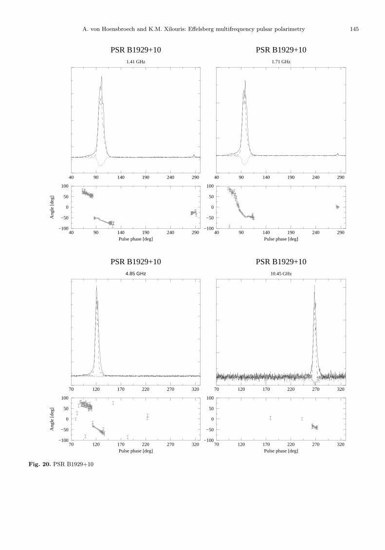
havior. The cross coupling parameters ε and θ are readilyobtained from the amplitude and phase of a cosine wavefit to the data. Two well studied and bright pulsars, PSRB1929+10 and PSR B0355+54, were chosen as calibratorsand were observed for a small range of parallactic angleduring each observing run. Those pulsars apart from ex-hibiting standard polarization profiles, involve a numberof different polarization states with strong linear polar-ization and small circular, with the associated PPA welldefined. This provides a good estimate of the ratio Vobs.

Lobs.

as a function of φ. The fitted parameters ε and θ wereused to correct the L and V waveforms as well as the pul-sar intrinsic polarization position angle curve by solvingthe system of Eqs. (21) for the true polarization states.The results from a two year monitoring of the polariza-tion properties for all of the receivers that we used arepresented in Table 1. The cross-coupling amplitude wasless than 10% and quite stable within the time intervalsthat the instrumental set-up remained unchanged.

A known source of depolarization is Faraday rotationwhich occurs both in the galactic interstellar medium andin the Earth’s ionosphere. These effects combine with un-equal phase delays between the two polarization channelsof the instrumental setup to effectively depolarize the in-cident polarization state. In all cases, this effect resultsfrom different propagation velocities between the left-handand right-hand circularly polarized components. The neteffect of either true or instrumental Faraday rotation isthat the position angle of the linear polarization becomesfrequency dependent. Across some finite bandwidth, thedispersion of the position angle results in a net loss oflinear polarization. Both the shape and the width of theIF filters that are used to form gain corrected Stokes pa-rameters play an important role in a quantitative deter-mination of the depolarization. Following the analysis ofRankin et al. (1975) for square filters, the largest amountsof depolarization estimated for the highest rotation mea-sure pulsars in our sample at 1.4 GHz is between 3 to8% with the rest of the sources less than 1%. At frequen-cies higher than 1.4 GHz, this effect was negligible. TheFaraday-induced position angle rotation across the band-widths used was between 16◦ and 32◦ for the high RMpulsars in our sample. Most of the RMs in our samplewere low and in these cases less than 5◦ of rotation werecalculated. The instrumentally-induced position angle ro-tation across the bandwidths used is proportional to thedifference in electrical path length between the two circu-lar channels. Severe depolarization would occur if the timedelay exceeded the reciprocal of the observing bandwidth.For the 1.4 GHz setup, a difference in the electrical path


of 7.5 m would be required to cause severe instrumentaldepolarization.

4. Results

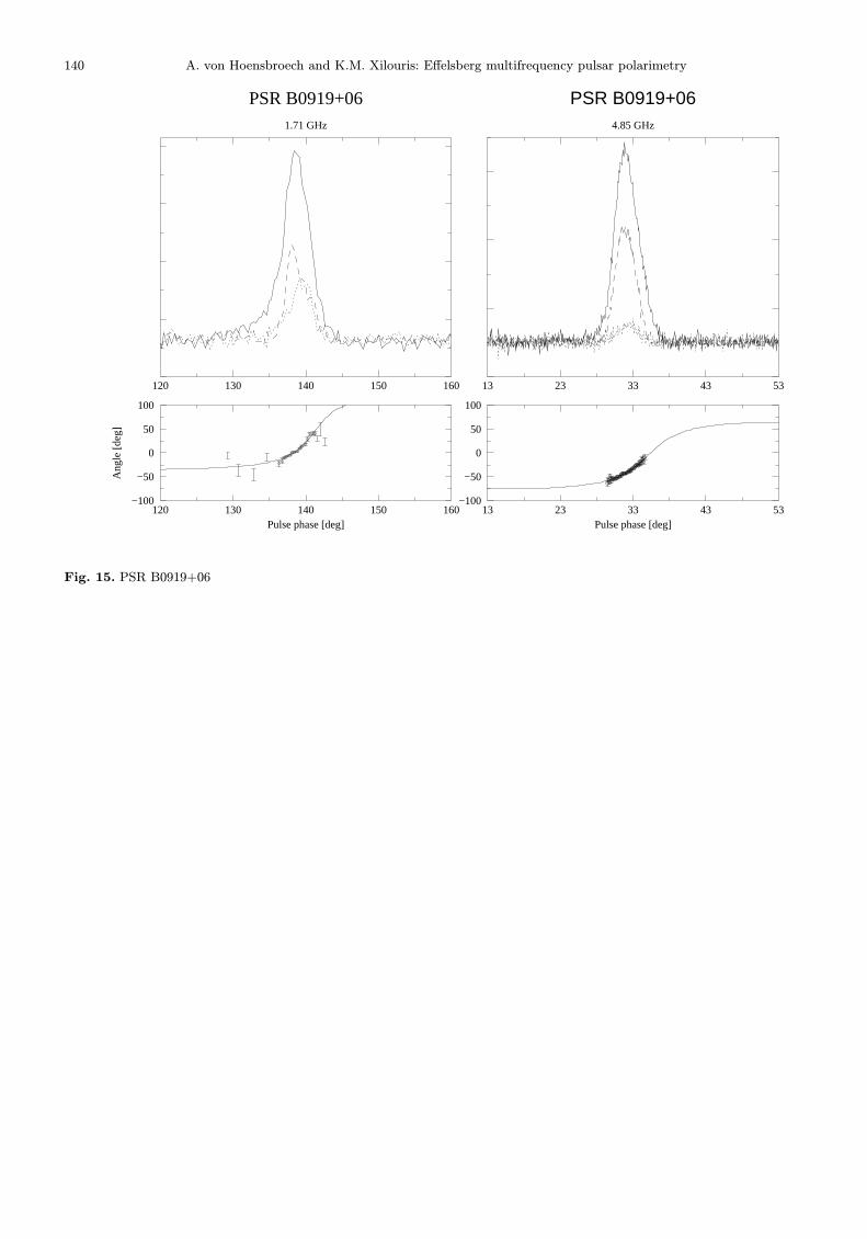
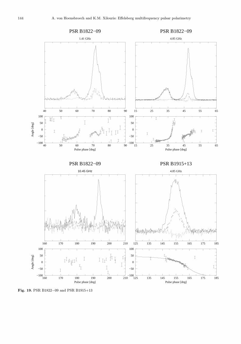
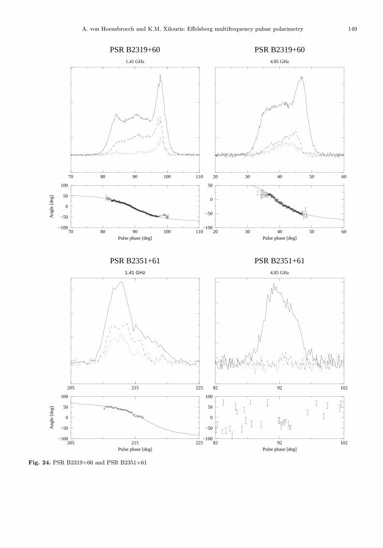
An elaborate procedure was developed to ensure highquality pulsar polarimetry at wide bandwidths. Thisscheme has served reasonably well for detecting instru-mental errors on-line and for monitoring of the polariza-tion characteristics of our instrumental set-up for a periodof 2 years at the Effelsberg radio telescope. This procedurewas applied to 64 polarization profiles of 28 pulsars atcm-wavelengths. The calibrated polarization profiles areshown in Figs. 5-24 at the end of this section. Wheneverpossible, a fit of the Rotating-Vector-Model (RVM; e.g.Manchester & Taylor 1977) to the PPA curve of eachsource was made which enabled a determination of theviewing geometry of each system. The viewing geometryof each system is presented in Table 3 while the fits aresuperimposed on the polarization plots of Figs. 5-24. Themagnetic inclination angle α and the the impact parame-ter σ (the closest approach of the magnetic axis to the line-of-sight trajectory) are listed in Cols. 3 and 4 of Table 3 re-spectively, together with their estimated errors. The valuesof α have a certain ambiguity, because the parameters αand σ are highly correlated. This accounts for the large er-rors associated with these parameters. Thus, it is doubtfulwhether α always represents the “true” value of the mag-netic inclination. However, the BCW method that we haveused to determine emission heights at cm-wavelengths isinsensitive to the magnetic inclination. Therefore, our re-sults for the emission altitudes are not effected by thisambiguity. The derived heights are presented in the lastcolumn of Table 3. A detailed description of the fittingprocedure and its associated complications as well as adiscussion of our findings is presented in von Hoensbroech& Xilouris (1997).

In Table 3, quantitative polarization parameters aresummarized. The cut-level given in Col. 3 represents theheight above the noise (relative to the peak of the respec-tive outer component) where the outer edges of a pro-file were found. The resulting width of the profile is thenlisted in the next column. The linear and circular inten-sities are the relative polarized power integrated over thiswidth. Low polarization levels which become progressivelyless with frequency are found for most of our sources.Additionally, the flux density was determined and listedin Table 3, together with the integration time of the par-ticular observation.

Polarization plots for all the pulsars in our sample atmany frequencies are presented in Figs. 5-24. For each po-larization plot, the upper panel contains the total intensityI (solid line), the linearly polarized L (dashed line), andthe circularly polarized V (dotted line) intensities. Thelower panel contains the derived PPA curve with associ-ated errors at each point. The points were chosen so that

Table 2. The derived geometry and emission heights for eachpulsar as a result the fitting procedure. The magnetic inclina-tion, α, is the angle between the rotation- and the magneticaxis, while σ represents the impact angle between the magneticaxis and the line-of-sight. The emission height derived with theBCW-method is presented on the last column

PSR B Freq. α σ rdelay

[GHz] [◦] [◦] [km]

0136 + 57 4.85 96.0±15.0 −3.6±15.0 530±740301 + 19 4.85 94.3±15.0 −13.9±15.0 1416±8880329 + 54 10.45 94.0±15.0 −12.4±15.0 −23±1920355 + 54 1.71 53.1±80.0 −8.6±4.0 303±76

4.85 155.8±80.0 −2.7±4.0 214±12010.45 111.9±80.0 −10.2±6.0 128±211

0525 + 21 1.41 135.8±60.0 1.3±.2 224±311.71 66.3±80.0 2.0±1.0 736±4674.85 17.8±70.0 0.6±2.0 378±174

0535 + 28 1.41 108.5±30.0 −11.5±6.0 619±964.85 79.5±15.0 −18.5±15.0 240±267

0540 + 23 1.41 162.5±80.0 −3.5±6.0 612±814.85 80.3±20.0 10.0±10.0 730±15510.45 101.1±90.0 −8.3±6.0 297±167

0740 − 28 1.41 96.2±20.0 −16.0±15.0 210±294.85 78.2±15.0 14.8±15.0 268±3810.45 47.3±90.0 −6.9±5.0 225±218

0809 + 74 1.71 93.4±10.0 −9.8±15.0 1267±4384.85 174.3±90.0 −0.7±7.5 447±725

0823 + 26 1.41 89.8±25.0 1.0±0.2 37±531.71 82.3±80.0 1.7±1.5 107±674.85 97.5±15.0 −12.1±15.0 80±21

0919 + 06 1.71 90.4±80.0 2.9±2.0 314±874.85 48.0±80.0 2.9±2.5 247±68

0950 + 08 1.41 −0.7±15.0 1.0±15.0 432±2494.85 −26.9±90.0 4.1±5.0 159±348

1133 + 16 1.41 26.9±90.0 2.8±4.4 452±1021.71 103.6±80.0 4.1±2.5 505±1464.85 33.0±80.0 3.1±4.0 426±165

1915 + 13 4.85 90.7±12.5 −9.3±15.0 346±751946 + 35 4.85 52.9±80.0 4.2±3.0 133±1682016 + 28 4.85 89.8±15.0 4.2±15.0 159±1812021 + 51 1.41 22.5±90.0 1.2±2.5 787±42

1.71 21.0±80.0 3.1±5.0 450±914.85 22.4±90.0 4.0±5.0 389±13710.45 87.9±80.0 5.8±3.0 590±182

2045 − 16 4.85 89.5±15.0 −1.5±15.0 443±2322154 + 40 4.85 101.1±15.0 −16.0±15.0 904±4702319 + 40 1.41 102.3±80.0 −8.1±4.0 −418±223

4.85 89.9±15.0 −6.5±15.0 −1242±5402351 + 61 1.41 61.2±80.0 −2.9±2.0 379±241

the linear polarization was 3 σ above the noise level. Incertain cases where significant off-pulse emission was de-tected, this criterion was relaxed. When a fit of the RVMto the data was applied, the fitted function was overplot-ted to the data as a solid line. The points which wereconsidered for these fits are marked with circles.

5. Conclusions

Carefully conducted polarimetric observations still sufferfrom polarization state changes due to gain and phase de-lays, cross-coupling, and depolarization in the observing


Table 3. The polarization parameters for each frequency for the pulsars in our sample

Pulsar Freq. Cut-level Width Linear Circular Time Flux[GHz] [%] [◦] [%] [%] [min] [mJy]

PSR B0136+57 4.85 10 12.5±2.6 54.0±1.0 12.1±1.5 20 0.17PSR B0301+19 4.85 10 14.0±1.6 10.3±3.0 5.5±5.0 45 3.09PSR B0329+54 1.41 2 30.7±1.1 24.1±0.1 36.3±0.1 10 90.9

1.71 7 28.8±1.2 21.0±0.0 9.3±0.0 10 39.44.85 7.6 27.4±0.9 12.3±0.2 7.4±0.2 10 20.510.45 33 22.2±1.7 12.9±2.3 7.3±3.3 15 1.75

PSR B0355+54 1.71 10 35.2±4.8 53.9±2.1 4.7±0.4 1 33.44.85 5 33.5±6.0 69.3±1.3 8.2±1.0 10 3.3610.45 5 31.4±21.7 41.9±5.5 0.9±5.7 15 3.37

PSR B0450+55 1.41 5 33.5±3.0 35.2±0.9 11.0±1.4 5 21.94.85 10 29.3±6.1 44.8±1.5 6.0±1.6 15 1.78

PSR B0525+21 1.41 1 21.1±0.3 40.4±0.2 3.9±0.3 3 85.71.71 10 17.9±0.7 30.9±1.5 3.4±1.1 10 8.84.85 3 17.2±0.4 20.6±0.6 1.0±0.9 90 0.10

PSR B0535+28 1.41 15.9 29.7±4.5 82.9±1.7 1.0±0.9 13 3.14.85 16.9 31.9±11.3 51.1±2.8 1.0±0.9 15 0.94

PSR B0540+23 1.41 3 33.7±4.9 46.9±0.9 3.8±0.4 3 22.24.85 7 28.4±4.9 29.7±1.2 13.4±1.3 20 2.1910.45 10 22.5±4.2 6.2±7.1 3.6±7.6 35 1.16

PSR B0740-28 1.41 4 19.6±2.1 77.0±0.5 10.7±0.5 5 20.74.85 7 20.3±2.0 63.4±1.7 8.5±1.9 60 2.4710.45 10 14.2±8.8 39.9±12.2 4.3±12.9 30 0.65

PSR B0809+74 1.71 8 29.0±3.4 23.4±2.5 9.1±2.6 8 10.74.85 10 26.7±3.6 14.1±1.0 3.1±1.6 15 2.54

PSR B0823+26 1.41 5 9.3±1.1 20.0±3.1 3.4±2.7 3 12.81.71 5 8.0±1.4 22.8±5.9 2.8±6.9 10 4.14.85 1 13.8±1.6 17.3±0.9 0.7±1.4 30 2.63

PSR B0919+06 1.71 8 10.5±2.0 38.5±10.6 27.5±13.5 5 3.24.85 7 7.9±1.4 47.3±2.6 4.6±3.0 45 0.63

PSR B0950+08 1.41 1 72.4±4.7 14.8±0.1 3.7±0.1 5 80.44.85 4 45.3±8.6 8±0.8 0.3±1.3 10 41.310.45 15 23.8±11.9 5.3±6.4 3.2±9.2 50 8.61

PSR B1133+16 1.41 8 10.9±0.6 15.8±0.4 1.8±0.7 5 19.51.71 4 11.6±0.3 12.1±0.2 5.4±0.3 10 24.54.85 8 9.4±0.5 10.4±0.3 2.4±0.4 20 4.3810.45 8 9.8±6.9 7.8±23.9 10.4±31.2 20 0.45

setup. A detailed analysis is presented here for an addingand a multiplying polarimeter used with three different re-ceivers with the Effelsberg radio telescope to perform highquality polarimetry. The analysis consists of a method todynamically detect and account for the differential gainsin the observing system. The gain monitoring is basedon the injection of a calibration signal prior to the po-larizer. This signal is synchronous to the pulsar periodand is dynamically adjusted for imbalances between thepolarization channels if needed. Once gain corrected dataare available, a detailed procedure is followed to accountfor cross-coupling effects. These effects are then removedfrom the measurements. Using the method we have de-scribed, the performance of the observing system can beroutinely evaluated. This reduction procedure providedevidence for the stability of the polarization characteris-tics of the instrumental set-up used, and ensured the highquality of the polarization data. The sample of 28 pulsarsat many frequencies presented here was also used to de-rive emission altitudes based on a method developed by

Blaskiewicz et al. (1991) and the results and interpreta-tion are presented in von Hoensbroech & Xilouris (1997).The polarization data presented here comprise a reliabledatabase at cm-wavelengths which can facilitate furtherstudies of polarization effects of pulsars at high frequen-cies.

Acknowledgements. We want to express our gratitude to Drs.M. Kramer, A. Jessner and R. Wielebinski for their con-stant help, support and valuable advice. We are in particulargrateful to C. Salter for extremely helpful suggestions. AreciboObservatory is operated by Cornell University under coopera-tive agreement with NSF.

References

Blaskiewicz M., Cordes J., Wasserman J., 1991, ApJ 370, 643Cordes J., 1978, ApJ 222, 1006Hoensbroech A. von, Xilouris K.M., 1996 (accepted)Kramer M., 1995, PhD-thesis, University of BonnKraus J.D., 1966, Radio Astronomy. McGraw-Hill Book

Company, p. 122


Table 3. continued

Pulsar Freq. Cut-level Width Linear Circular Time Flux[GHz] [%] [◦] [%] [%] [min] [mJy]

PSR B1237+25 1.41 2 15.4±0.5 51.0±0.2 16.0±0.2 8 28.34.85 5 13.6±1.4 13.5±1.7 5.2±2.1 20 0.79

PSR B1642-03 1.41 1.6 17.9±3.1 11.2±1.9 9.2±2.4 3 15.24.85 10 18.6±3.3 8.6±3.5 1.2±3.5 25 1.10

PSR B1822-09 1.41 18 22.8±2.2 32.9±1.1 11.6±1.2 5 6.34.85 10 23.5±1.7 32.1±1.7 2.3±0.5 15 4.7610.45 30 19.3±5.5 86.7±76.5 36.3±71.6 25 0.26

PSR B1915+13 4.85 8 20.4±2.6 31.6±2.5 1.4±3.6 60 0.50PSR B1929+10 1.41 1 53.8±4.1 71.9±0.1 12.5±0.1 3 233.3

1.71 1 52.1±4.8 71.5±0.2 13.8±0.2 2 160.64.85 1 41.8±6.0 65.7±0.5 0.6±0.5 5 6.8010.45 10 14.8±3.0 43.1±4.1 2.9±5.0 20 2.23

PSR B1946+35 4.85 10 18.7±1.4 12.6±2.7 0.3±4.3 20 0.50PSR B2016+28 4.85 10 15.1±1.9 0.8±1.7 3.0±2.1 20 0.85PSR B2020+28 4.85 2 18.3±0.9 14.3±0.3 5.7±0.3 20 1.64

10.45 8 13.7±0.5 5.4±6.4 8.4±10.7 45 0.77PSR B2021+51 1.41 2 23.8±1.1 28.6±0.1 3.6±0.1 5 52.3

1.71 3 22.2±2.2 38.8±0.3 11.0±0.5 5 30.84.85 3 19.3±2.0 22.7±0.3 0.7±0.3 25 9.7310.45 10 12.7±2.6 29.6±6.3 0.7±8.3 10 1.22

PSR B2045-16 4.85 10 14.2±0.4 9.2±1.6 2.2±2.1 20 1.06PSR B2154+40 4.85 10 23.9±3.0 25.1±4.8 0.7±6.2 20 0.64PSR B2310+42 1.41 5 17.3±1.6 28.4±2.0 4.4±1.6 30 12.4

4.85 10 14.3±0.9 6.9±0.4 2.7±1.0 30 0.20PSR B2319+60 1.41 4 23.3±0.9 40.1±0.3 9.5±0.1 8 27.1

4.85 5 20.9±1.6 21.3±0.9 9.4±1.5 20 0.24PSR B2351+61 1.41 7 12.0±1.4 64.6±10.0 22.8±11.3 20 1.1

4.85 10 9.5±3.1 6.8±3.8 1.8±4.9 20 0.08

Manchester R.N., Taylor J.H., 1977, Pulsars, Freeman, SanFrancisco

Radhakrishnan V., Cooke D.J., 1969, Astrophys. Lett. 3, 225Rankin J.M., Campbell D.B., Spangler S.R., 1975, NAIC-

Reports, Vol. 44

Saikia D.J., Salter C.J., 1988, ARA&A 26, 93Stinebring D.R., Cordes J.M., Weisberg J.M., Rankin J.M.,

Boriakoff V., 1984, ApJS 55, 27Turlo S., Fokert T., Sieber W., 1985, A&A 142, 181Xilouris K.M., 1991, A&A 248, 323


30 40 50Pulse phase [deg]

−100

−50

0

50

100

Ang

le [d

eg]

30 40 50

PSR B0136+574.85 GHz

40 50 60 70Pulse phase [deg]

−100

−50

0

50

100

40 50 60 70

PSR B0301+194.85 GHz

Fig. 5. PSR B0301+57 and PSR B0301+19. For each profile two panels are plotted. The upper one shows total power (solid),linearly- (dashed) and circularly [V = LHC− RHC] (dotted) polarized intensity. The lower plot shows the derived PPA-pointswith their error bars. In all cases only such PPA-points are shown which have a signal–to–noise ratio above a certain level,depending on the polarisation of the pulsar. In those cases when a fit of the RVM to the data was applied, the fitted functionis plotted. The points which were considered for the fits are marked with circles


35 45 55 65 75Pulse phase [deg]

−100

−50

0

50

100

Ang

le [d

eg]

35 45 55 65 75

PSR B0329+544.85 GHz


−100

−50

0

50

100

Ang

le [d

eg]

21 31 41 51 61

PSR B0329+541.41 GHz

70 80 90 100 110Pulse phase [deg]

−100

−50

0

50

100

70 80 90 100 110

PSR B0329+5410.55 GHz

273Pulse phase [deg]

−100

−50

0

50

100

273 283 293 303 313

PSR B0329+541.71 GHz

Fig. 6. PSR B0329+54


72 82 92 102 112 122 132Pulse phase [deg]

−100

−50

0

50

100

Ang

le [d

eg]

72 82 92 102 112 122 132

PSR B0355+5410.55 GHz

40 50 60 70 80 90 100Pulse phase [deg]

−100

−50

0

50

100

Ang

le [d

eg]

40 50 60 70 80 90 100

PSR B0355+541.71 GHz

75 85 95 105 115 125 135Pulse phase [deg]

−100

−50

0

50

100

75 85 95 105 115 125 135

PSR B0355+544.85 GHz

Fig. 7. PSR B0355+54


200 210 220 230 240 250 260 270Pulse phase [deg]

−100

−50

0

50

100

Ang

le [d

eg]

200 210 220 230 240 250 260 270

PSR B0450+551.41 GHz

30 40 50 60 70 80 90 100Pulse phase [deg]

−100

−50

0

50

100

30 40 50 60 70 80 90 100

PSR B0450+554.85 GHz

Fig. 8. PSR B0450+55



−100

−50

0

50

100

Ang

le [d

eg]

95 105 115 125

PSR B0525+214.85 GHz


−100

−50

0

50

100

Ang

le [d

eg]

198 208 218 228

PSR B0525+211.41 GHz


−100

−50

0

50

100

40 50 60 70

PSR B0525+211.71 GHz

Fig. 9. PSR B0525+21


50.0 70.0 90.0 110.0Pulse phase [deg]

-100.0

-50.0

0.0

50.0

100.0

Ang

le [

deg]

50.0 70.0 90.0 110.0

PSR J0538+281.41 GHz


-100

-50

0

50

100

55 75 95 115

PSR J0538+284.85 GHz

Fig. 10. PSR J0538+28


290 300 310 320 330 340 350Pulse phase [deg]

−100

−50

0

50

100

Ang

le [d

eg]

290 300 310 320 330 340 350

PSR B0540+2310.45 GHz

100 110 120 130 140 150 160Pulse phase [deg]

−100

−50

0

50

100

Ang

le [d

eg]

100 110 120 130 140 150 160

PSR B0540+231.41 GHz

60 70 80 90 100 110 120Pulse phase [deg]

−100

−50

0

50

100

60 70 80 90 100 110 120

PSR B0540+234.85 GHz

Fig. 11. PSR B0540+23



−100

−50

0

50

100

Ang

le [d

eg]

125 135 145 155

PSR B0740−2810.55 GHz


−100

−50

0

50

100

Ang

le [d

eg]

55 65 75 85

PSR B0740−281.41 GHz


−100

−50

0

50

100

60 70 80 90

PSR B0740−284.85 GHz

Fig. 12. PSR B0740−28


35.0 45.0 55.0 65.0 75.0 85.0 95.0Pulse phase [deg]

−100.0

−50.0

0.0

50.0

100.0

Ang

le [d

eg]

35.0 45.0 55.0 65.0 75.0 85.0 95.0

PSR B0809+744.85 GHz

60 70 80 90 100 110Pulse phase [deg]

−100

−50

0

50

100

Ang

le [d

eg]

60 70 80 90 100 110

PSR B0809+741.41 GHz

60 70 80 90 100 110Pulse phase [deg]

−100

−50

0

50

100

60 70 80 90 100 110

PSR B0809+741.71 GHz

Fig. 13. PSR B0809+74



−100

−50

0

50

100

Ang

le [d

eg]

250 260 270

PSR B0823+264.85 GHz


−100

−50

0

50

100

Ang

le [d

eg]

48 58 68

PSR B0823+261.41 GHz


−100

−50

0

50

100

57 67 77

PSR B0823+261.71 GHz

Fig. 14. PSR B0823+26


120 130 140 150 160Pulse phase [deg]

−100

−50

0

50

100

Ang

le [d

eg]

120 130 140 150 160

PSR B0919+061.71 GHz


−100

−50

0

50

100

13 23 33 43 53

PSR B0919+064.85 GHz

Fig. 15. PSR B0919+06


40 90 140 190 240 290Pulse phase [deg]

−100

−50

0

50

100

Ang

le [d

eg]

40 90 140 190 240 290

PSR B0950+0810.45 GHz

70 120 170 220 270 320Pulse phase [deg]

−100

−50

0

50

100

Ang

le [d

eg]

70.0 170.0 270.0

PSR B0950+081.41 GHz

70 120 170 220 270 320Pulse phase [deg]

−100

−50

0

50

100

70.0 170.0 270.0

PSR B0950+084.85 GHz

Fig. 16. PSR B0950+08



-100

-50

0

50

100

Ang

le [

deg]

20 30 40

PSR B1133+164.85 GHz


-100

-50

0

50

100

Ang

le [

deg]

57.0 67.0 77.0

PSR B1133+161.41 GHz


-100

-50

0

50

100

213 223 233

PSR B1133+1610.45 GHz


-100

-50

0

50

100

15 25 35

PSR B1133+161.71 GHz

Fig. 17. PSR B1133+16


155 165 175 185 195Pulse phase [deg]

−100

−50

0

50

100

Ang

le [d

eg]

155 165 175 185 195

PSR B1642−031.41 GHz


−100

−50

0

50

100

Ang

le [d

eg]

55 65 75

PSR B1237+251.41 GHz

107 117 127 137 147Pulse phase [deg]

−100

−50

0

50

100

107 117 127 137 147

PSR B1642−034.85 GHz


−100

−50

0

50

100

54 64 74

PSR B1237+254.85 GHz

Fig. 18. PSR B1237+25 and PSR B1642-03


160 170 180 190 200 210Pulse phase [deg]

−100

−50

0

50

100

Ang

le [d

eg]

160 170 180 190 200 210

PSR B1822−0910.45 GHz

40 50 60 70 80 90Pulse phase [deg]

−100

−50

0

50

100

Ang

le [d

eg]

40 50 60 70 80 90

PSR B1822−091.41 GHz

125 135 145 155 165 175 185Pulse phase [deg]

−100

−50

0

50

100

125 135 145 155 165 175 185

PSR B1915+134.85 GHz

15 25 35 45 55 65Pulse phase [deg]

−100

−50

0

50

100

15 25 35 45 55 65

PSR B1822−094.85 GHz

Fig. 19. PSR B1822−09 and PSR B1915+13


70 120 170 220 270 320Pulse phase [deg]

−100

−50

0

50

100

Ang

le [d

eg]

70 120 170 220 270 320

PSR B1929+104.85 GHz

40 90 140 190 240 290Pulse phase [deg]

−100

−50

0

50

100

Ang

le [d

eg]

40 90 140 190 240 290

PSR B1929+101.41 GHz

70 120 170 220 270 320Pulse phase [deg]

−100

−50

0

50

100

70 120 170 220 270 320

PSR B1929+1010.45 GHz

40 90 140 190 240 290Pulse phase [deg]

−100

−50

0

50

100

40 90 140 190 240 290

PSR B1929+101.71 GHz

Fig. 20. PSR B1929+10



−100

−50

0

50

100

Ang

le [d

eg]

35 45 55 65

PSR B2020+284.85 GHz

85 95 105 115 125Pulse phase [deg]

−100

−50

0

50

100

Ang

le [d

eg]

85 95 105 115 125

PSR B1946+354.85 GHz


−100

−50

0

50

100

152 162 172 182

PSR B2020+2810.45 GHz


−100

−50

0

50

100

25 35 45 55

PSR B2016+284.85 GHz

Fig. 21. PSR B1946+35, PSR B2016+28 and PSR B2020+28



−100

−50

0

50

100

Ang

le [d

eg]

20 30 40 50 60

PSR B2021+514.85 GHz

75 85 95 105 115Pulse phase [deg]

−100

−50

0

50

100

Ang

le [d

eg]

75 85 95 105 115

PSR B2021+511.41 GHz

130 140 150 160 170Pulse phase [deg]

−100

−50

0

50

100

130 140 150 160 170

PSR B2021+5110.45 GHz

65 75 85 95 105 115Pulse phase [deg]

−100

−50

0

50

100

65 75 85 95 105

PSR B2021+511.71 GHz

Fig. 22. PSR B2021+51



−100

−50

0

50

100

Ang

le [d

eg]

95 105 115 125

PSR B2310+421.41 GHz


−100

−50

0

50

100

Ang

le [d

eg]

48 58 68

PSR B2045−164.85 GHz


−100

−50

0

50

100

37 47 57 67

PSR B2310+424.85 GHz

185 195 205 215 225Pulse phase [deg]

−100

−50

0

50

100

185 195 205 215 225

PSR B2154+404.85 GHz

Fig. 23. PSR B2054−16, PSR B2154+40 and PSR B2310+42



−100

−50

0

50

100

Ang

le [d

eg]

205 215 225

PSR B2351+611.41 GHz

70 80 90 100 110Pulse phase [deg]

−100

−50

0

50

100

Ang

le [d

eg]

70 80 90 100 110

PSR B2319+601.41 GHz


−100

−50

0

50

100

82 92 102

PSR B2351+614.85 GHz


−100

−50

0

50

20 30 40 50 60

PSR B2319+604.85 GHz

Fig. 24. PSR B2319+60 and PSR B2351+61

effelsberg multifrequency pulsar polarimetry · a. von hoensbroech and k.m. xilouris: e elsberg...

Documents