effects of wave shape on sheet flow sediment transport of wave shape on sheet flow sediment...

Effects of wave shape on sheet flow sediment transport

Tian-Jian Hsu1

Center for Applied Coastal Research, University of Delaware, Newark, Delaware, USA

Daniel M. Hanes2

Western Coastal and Marine Geology, U.S. Geological Survey Pacific Science Center, Santa Cruz, California, USA

Received 30 July 2003; revised 19 March 2004; accepted 1 April 2004; published 25 May 2004.

[1] A two-phase model is implemented to study the effects of wave shape on the transportof coarse-grained sediment in the sheet flow regime. The model is based on balanceequations for the average mass, momentum, and fluctuation energy for both the fluid andsediment phases. Model simulations indicate that the responses of the sheet flow, such asthe velocity profiles, the instantaneous bed shear stress, the sediment flux, and thetotal amount of the mobilized sediment, cannot be fully parameterized by quasi-steadyfree-stream velocity and may be correlated with the magnitude of local horizontal pressuregradient (or free-stream acceleration). A net sediment flux in the direction of waveadvance is obtained for both skewed and saw-tooth wave shapes typical of shoaled andbreaking waves. The model further suggests that at critical values of the horizontalpressure gradient, there is a failure event within the bed that mobilizes more sediment intothe mobile sheet and enhances the sediment flux. Preliminary attempts to parameterizethe total bed shear stress and the total sediment flux appear promising. INDEX TERMS:

4558 Oceanography: Physical: Sediment transport; 4546 Oceanography: Physical: Nearshore processes; 3022

Marine Geology and Geophysics: Marine sediments—processes and transport; 4568 Oceanography: Physical:

Turbulence, diffusion, and mixing processes; KEYWORDS: sediment transport, bed shear stress, sheet flow

Citation: Hsu, T.-J., and D. M. Hanes (2004), Effects of wave shape on sheet flow sediment transport, J. Geophys. Res., 109,

C05025, doi:10.1029/2003JC002075.

1. Introduction

[2] One of the most important but relatively unknownaspects of wave-induced sediment transport and cross-shoreprofile evolution is the mechanism through which wavestransport sediment onshore to counteract the effects ofgravity. A key parameter for cross-shore sediment transportunder breaking and near-breaking waves is the shape of thenear-bed wave orbital velocity. It is generally believed that askewed velocity field can cause a net cross-shore transportof sediment without a net transport of water, though thedetailed mechanics of this process are not well understood.From a parameterization point of view, there is significantexperimental evidence that flow acceleration, which servesas a proxy for horizontal pressure gradient in coastal bottomboundary layer, has an effect on sediment transport. Thisevidence derives from U-tube experiments [e.g., King,1990] and field measurements in the surf zone [e.g., Hanesand Huntley, 1986; Gallagher et al., 1998] and in the swash[e.g., Butt and Russell, 1999; Puleo et al., 2003]. Motivatedin part by King’s [1990] measured sediment transport rates

under saw-tooth shaped waves, Nielsen [1992] proposed anempirical formula that estimates the Shields parameterbased on both flow velocity and acceleration. More recently,Nielsen [2002] and Nielsen and Callaghan [2003] imple-mented a modified version of the formula for the Shieldsparameter proposed by Nielsen [1992] and applied it topredict sediment transport rate measurements in the swashzone [Masselink and Hughes, 1998] and to measurements ofsheet flow in a large-scale wave flume under non-breakingwaves [Dohmen-Janssen and Hanes, 2002]. Although theformula proposed by Nielsen and his colleagues hasachieved a certain degree of success in predicting thesediment transport rate under unsteady conditions, a morecomplete theoretical background for the unsteady effect onbed shear stress and corresponding sediment transport iswarranted.[3] Numerical simulations of bedload sediment transport

have also indicated that the sediment flux is influenced byflow acceleration. Drake and Calantoni [2001] proposed aparameterization of acceleration effects based upon discreteelement simulations. Recently, Hoefel and Elgar [2003] usethe acceleration skewness parameterization suggested byDrake and Calantoni [2001] in combination with thecommonly used energetics-based total load formula ofBailard [1981]. They are able to predict the beach profileevolution, including both onshore and offshore sandbarmigrations, over a 45-day period during the Duck94 experi-ments [Elgar et al., 2001].

JOURNAL OF GEOPHYSICAL RESEARCH, VOL. 109, C05025, doi:10.1029/2003JC002075, 2004

1Now at Applied Ocean Physics and Engineering Department, WoodsHole Oceanographic Institution, Woods Hole, Massachusetts, USA.

2Also at Department of Civil and Coastal Engineering, University ofFlorida, Gainesville, Florida, USA.

Copyright 2004 by the American Geophysical Union.0148-0227/04/2003JC002075$09.00

C05025 1 of 15

Report Documentation Page Form ApprovedOMB No. 0704-0188

Public reporting burden for the collection of information is estimated to average 1 hour per response, including the time for reviewing instructions, searching existing data sources, gathering andmaintaining the data needed, and completing and reviewing the collection of information. Send comments regarding this burden estimate or any other aspect of this collection of information,including suggestions for reducing this burden, to Washington Headquarters Services, Directorate for Information Operations and Reports, 1215 Jefferson Davis Highway, Suite 1204, ArlingtonVA 22202-4302. Respondents should be aware that notwithstanding any other provision of law, no person shall be subject to a penalty for failing to comply with a collection of information if itdoes not display a currently valid OMB control number.

1. REPORT DATE 2004 2. REPORT TYPE

3. DATES COVERED 00-00-2004 to 00-00-2004

4. TITLE AND SUBTITLE Effects of Wave Shape on Sheet Flow Sediment Transport

5a. CONTRACT NUMBER

5b. GRANT NUMBER

5c. PROGRAM ELEMENT NUMBER

6. AUTHOR(S) 5d. PROJECT NUMBER

5e. TASK NUMBER

5f. WORK UNIT NUMBER

7. PERFORMING ORGANIZATION NAME(S) AND ADDRESS(ES) Center for Applied Coastal Research,University of Delaware,Newark,DE,19711

8. PERFORMING ORGANIZATIONREPORT NUMBER

9. SPONSORING/MONITORING AGENCY NAME(S) AND ADDRESS(ES) 10. SPONSOR/MONITOR’S ACRONYM(S)

11. SPONSOR/MONITOR’S REPORT NUMBER(S)

12. DISTRIBUTION/AVAILABILITY STATEMENT Approved for public release; distribution unlimited

13. SUPPLEMENTARY NOTES

14. ABSTRACT

15. SUBJECT TERMS

16. SECURITY CLASSIFICATION OF: 17. LIMITATION OF ABSTRACT Same as

Report (SAR)

18. NUMBEROF PAGES

15

19a. NAME OFRESPONSIBLE PERSON

a. REPORT unclassified

b. ABSTRACT unclassified

c. THIS PAGE unclassified

Standard Form 298 (Rev. 8-98) Prescribed by ANSI Std Z39-18

[4] On the contrary, recent laboratory measurements ofsediment transport under sheet flow condition in U-tubes orunder nonbreaking waves suggest that most of the transportoccurs in the concentrated region near the bed where thetime evolution of sediment concentration responses directlyto the free-stream velocity [e.g., Ribberink, 1998; Dohmen-Janssen and Hanes, 2002]. In this paper, we examine theresponses of sheet flow sediment transport under unsteadyforcing using a two-phase sheet flow model [Hsu et al.,2004]. We demonstrate that whether the sediment transportrate can be successfully parameterized by solely the mag-nitude of free-stream velocity strongly depends on the waveshape. We find that in general the time-dependent sedimenttransport is highly coherent with the corresponding instan-taneous bed shear stress. However, for certain wave shapes,the time evolution of bed shear stress cannot be parameter-ized by the instantaneous free-stream velocity in a quasi-steady sense.[5] After a brief description of the model, supplementary

model validations on the temporal variation of sedimenttransport rate are presented. To demonstrate that the sedi-ment transport process sometimes cannot be fully describedby solely the magnitude of free-stream velocity, we first usethe model to examine sheet flow under a prescribed free-stream velocity time history of a saw-tooth shape. Theseresults are further interpreted through an examination of thesediment-phase momentum equations to study the relevantphysical mechanisms responsible for our observation and toemphasize the effect of horizontal pressure gradient inmodeling unsteady sediment dynamics. We then investigateskewed waves typical in shallow water outside the surfzone. To further explore and quantify the relation betweenbed failure and sediment transport, the sediment transport isnext forced by using a free-stream velocity time historyshaped like a ramp, which drives the flow with a constantacceleration between two steady state conditions. Finally,motivated by the results of the two-phase model, we suggestnew directions toward an improved parameterization fornearshore sediment transport under sheet flow conditions.

2. Model Description

2.1. Two-Phase Equations

[6] The two-phase model of Hsu et al. [2004] will bebriefly summarized here for the convenience of the reader.We treat the mixture of grains and water as a two-phasemixture where each phase obeys the basic conservation ofmass, momentum, and energy. The fluid phase is treated asan incompressible liquid with mass density r f, and theparticle phase is treated as identical spheres with diameterd and mass density rs. The overall combined sheet flow isconsidered as that in a U-tube, in which the flow is assumedto be uniform in the flow direction and driven by aprescribed time history of free-stream velocity through thehorizontal pressure gradient.[7] The dynamics of the 1-dimensional fluid-granular

flow under consideration are assumed to be governed bythe two-phase conservation equations of fluid and sediment.The fluid and sediment phase continuity equations are

@r f 1� �cð Þ@t

þ @r f 1� �cð Þ~wf

@z¼ 0 ð1Þ

@rs�c@t

þ @rs�c~ws

@z¼ 0; ð2Þ

where z is normal to the channel bottom and ~w f and ~ws are,respectively, the z-components of the fluid and particlevelocities.[8] The horizontal (x) and vertical (z) components of the

fluid-phase momentum equations can be expressed as

@r f 1� �cð Þ~u f

@t¼� @r f 1� �cð Þ~u f ~wf

@z� 1� �cð Þ @

�Pf

@x

þ @t fxz

@z� b�c ~u f � ~us

� �ð3Þ

@r f 1� �cð Þ~wf

@t¼� @rf 1� �cð Þ~wf ~wf

@z� 1� �cð Þ @

�P f

@zþ @t f

zz

@z

þ r f 1� �cð Þg � b�c ~wf � ~ws� �

þ bnft@�c

@z; ð4Þ

where ~uf and ~us are, respectively, the x-components of thefluid and particle velocities, �P f is the fluid pressure, txz

f andtzzf are fluid phase stresses, including the fluid viscous stress

and the fluid Reynolds stresses, and g = �9.8 (m/s2) is thegravitational acceleration. The last two terms in equation (4)are the Favre-averaged [e.g., Drew, 1976] drag force with bdefined as

b ¼ r f Ur

d

18:0

Repþ 0:3

� �1

1� �cð Þn ; ð5Þ

in which

Ur ¼ffiffiffiffiffiffiffiffiffiffiffiffiffiffiffiffiffiffiffiffiffiffiffiffiffiffiffiffiffiffiffiffiffiffiffiffiffiffiffiffiffiffiffiffiffiffiffi~u f � ~usð Þ2þ ~wf � ~wsð Þ2

qð6Þ

is the magnitude of the relative velocity between the fluidand sediment phase, and Rep = r fUrd/mf is the particleReynolds number, with mf the fluid viscosity. In equation (5)the experimental results of Richardson and Zaki [1954] areadopted to incorporate the effect of sediment concentrationon the drag force, with n a coefficient depending on theparticle Reynolds number,

n ¼ 4:45Re�0:1p � 1; 1 � Rep < 500:

The last term in equation (4) is the modeled form for fluidturbulent suspension based on gradient transport, with nftthe fluid eddy viscosity.[9] The x and z components of the sediment-phase

momentum equations are

@rs�c~us

@t¼ � @rs�c~us~ws

@z� �c

@�P f

@xþ @tsxz

@zþ b�c ~u f � ~us

� �ð7Þ

@rs�c~ws

@t¼� @r s�c~ws~ws

@z� �c

@�P f

@zþ @t s

zz

@z

þ rs�cg þ b�c ~wf � ~ws� �

� bnft@�c

@z; ð8Þ

where txzs and tzz

s are the stresses of the sediment phase,including the small-scale particle (intergranular) stresses

C05025 HSU AND HANES: SHEET FLOW UNDER WAVES

2 of 15

C05025

and the Reynolds stresses of the Favre-averaged particlevelocities. Note that fluid and sediment phases exchangemomentum with each other through the equal andoppositely signed drag terms, and overall momentum isconserved.

2.2. Closure of Stresses

[10] The closures of the fluid Reynolds stresses and thesediment stresses are the essential components of thepresent two-phase sheet flow model. The fluid Reynoldsstresses are calculated by the eddy viscosity, which isfurther calculated by the fluid turbulence kinetic energy kfand its dissipation rate �f. The balance equations of kf and �fare derived from the two-phase theory that incorporatesessential influences from the sediment phase. Because thepresent kf -�f formulations are already presented in detail byHsu et al. [2003, 2004], they are not repeated here.[11] To calculate the sediment stress, a measure of the

strength of the particle velocity fluctuations,

Ks ¼1

2�ccDusiDu

si ; ð9Þ

the particle fluctuation energy, is introduced. This term isthe particle phase analog to turbulent kinetic energy in thefluid phase. The particle fluctuation energy is thencalculated by its balance equation,

rs@�cKs

@tþ @�cKs~w

s

@z

� �¼ tsxz

@~us

@zþ tszz

@~ws

@z� @Q

@z� g

þ 2b�c akf � Ks

� �; ð10Þ

with Q as the flux of the fluctuation energy and g as the rateof dissipation. The last term in equation (10) represents theeffect of the drag force, with a representing the degree ofcorrelation between the fluid velocity fluctuations andparticle velocity fluctuations,

a ¼ 1

1þ Tp=min TL;Tcð Þ ; ð11Þ

with TL = 0.165 kf /�f the fluid turbulence timescale[Elghobashi and Abou-Arab, 1983] and Tp = rs/b theparticle response time [Drew, 1976], which measures thetime to accelerate a single particle from rest to the velocityof surrounding fluid. The time between collisions Tc = lc/Ks

1/2

is estimated based on the strength Ks1/2 of sediment velocity

fluctuations and the mean free path lc =ffiffip

pd

24�cg0 �cð Þ of collidingparticles. Here g0(�c) is the contact value of the radialdistribution function [Torquato, 1995; Hsu et al., 2004]. Tosolve equation (10), we need to further incorporate closuresfor sediment stresses txz

s and tzzs , the flux of fluctuation

energy Q, and the rate of dissipation g.[12] Because the governing equations for sheet flow are

obtained from two averaging processes at different scales[e.g., Hsu et al., 2003], the closures in equation (10) mustincorporate intergranular components due to particle-parti-cle interactions and large-scale components of particlevelocity fluctuations induced by fluid turbulence [Youngand Leeming, 1997]. Following Jenkins and Hanes [1998],the intergranular interactions are assumed to be dominatedby particle collisions and a closure based on kinetic theory

of collisional granular flow [e.g., Jenkins and Savage, 1983]is implemented. On the other hand, since the large-scalesediment stress is influenced by fluid turbulence, we adopt aclosure similar to the one-equation fluid turbulence model.For the detailed mathematical representations of the clo-sures on txz

s , tzzs , Q and g, the readers are referred to Hsu et

al. [2004].[13] In the highly concentrated region nearest and

within the stationary bed, where the sediment concentra-tion is greater than the random loose-packing (c* = 57%),particles are in relatively long-term enduring contact.Since the fundamental assumption in the kinetic theoryrequires that the duration of contact between particlesmust be much smaller than the time between collisions,we need to modify the kinetic theory when modelingsediment stress in the region where sediment concentra-tion is between random loose-packing and random close-packing (c* = 63.5%).[14] For the particle shear stress, we modify the colli-

sional viscosity in the kinetic theory appropriate to theglass transition and adopt the experimental results ofBocquet et al. [2002], which suggest a much larger valueof collisional viscosity than that in the kinetic theorywhen the sediment concentration is greater than randomloose-packing. Hence the particle shear stress in theregion of enduring contact is modeled as an extremelyviscous granular continuum.[15] For particle normal stress, an additional component

tzzse due to enduring contact is incorporated into tzz

s when thesediment concentration is greater than random loose-pack-ing. We use the closure for tzz

se suggested by Jenkins et al.[1989], who analyzed homogeneously packed, identicalspheres in Herzian contact. They proposed a formula forparticle normal stress phrased in terms of the averagecompressive volume strain raised to the 3/2 power. Becausethe volume strain is not determined in the present model, weneed to modify the formula of Jenkins et al. [1989] in termsof sediment concentration,

tsezz ¼0; �c < c*mpd2 K �cð Þ�c �c� c*

� �cc* � �c � c*;

�ð12Þ

where m depends on material properties given in terms ofshear modulus and Poisson ratio of the granular materialand K(�c) is the coordination number, a function of sedimentconcentration, representing average numbers of particleswith which a particle is in contact. The specific mathemat-ical formulae of m and K(�c) are given by Hsu et al. [2004],and are not repeated here. The power c is considered to be anumerical coefficient in the model. Since c is stronglyrelated to the boundary conditions at bed, its value shall begiven in the next section.

2.3. Boundary Conditions

[16] The present model simulates sediment transportprocesses spanning the entire region from the stationary,porous sediment bed, where sediment particles are immo-bile, through the slowly shearing region of enduring particlecontact, to the rapid flow region of intense particle colli-sions, and finally to turbulent suspension. A description ofthe instantaneous (vertical) location of the bed (ILB), whichchanges in time according to the external flow forcing, must


3 of 15

C05025

be incorporated. We determine the movement of ILB byincorporating the Coulomb failure criterion,

tsxz ¼ tszz tanf; ð13Þ

where f is the friction angle of the sediment [see Hanesand Inman, 1985a, 1985b]. We note that throughmodifying the collisional viscosity to the glass transition,the total bed shear stress becomes part of the solution ofthe model that must respond to the unsteady forcing. Byapplying equations (12) and (13) at the stationary bedinterface with the known bed shear stress, the corre-sponding concentration at the bed, which we denote asfailure concentration c, can be calculated. Since thesediment concentration just above the immobile bed mustbe equal to c, the location of ILB can then be determinedso that the total amount of mobilized sediment is adjustedto satisfy the governing equations of the whole transienttwo-phase system. In addition, because the value of cmust be close to but not greater than the random close-packing, an appropriate numerical value for c can becalibrated. In the present model, c is set to be 5.5, whichgives c of about 62% to 63%. Within the porousimmobile bed, the sediment mean velocity and fluctuationenergy must vanish, and no-slip boundary conditions arespecified.[17] The proposed model is solved numerically with a

finite difference scheme. To drive the model with oscillatoryflow by a prescribed time history of free stream velocityu0(t), the horizontal pressure gradient is specified accordingto the acceleration of the free stream velocity,

1

rf@�Pf

@x¼ � duo tð Þ

dt: ð14Þ

2.4. Model Validation

[18] Hsu et al. [2004] validate the model with detailedvelocity and concentration profiles from laboratory experi-ments of Sumer et al. [1996] for steady flow and Asano[1995] for oscillatory flow. In this paper, we are interestedin the temporal variation of the volume sediment transportrate,

qs tð Þ ¼Z h

0

�c tð Þ~us tð Þdz; ð15Þ

calculated by integrating the horizontal sediment flux acrossthe water depth h with z = 0 located below the lowestmoving grains. Therefore we present comparisons betweenthe calculated qs, with that of Asano [1995] (Figure 1),under the prescribed free-stream velocity time history of asinusoidal wave,

u0 tð Þ ¼ U01 sin2pT

t

� �; ð16Þ

where U01 is the velocity amplitude and T is the oscillatoryperiod. The predicted instantaneous sediment transport ratesagree fairly well with the measured data. We note here thatno specific adjustments of the model parameters areconducted to fit the measured data set. Slightly largerdiscrepancies can be observed during the settling phase(t/T = 0.22 to 0.4) for case C1 and C2, which is due to theoverprediction of sediment velocity. More detailed com-parisons for sediment concentration and velocity at variousphases are presented by Hsu et al. [2004].

3. Asymmetric Saw-Tooth Wave Forcing

[19] The measured time histories of near-bed flow veloc-ity under broken waves often follows a saw-tooth shape[e.g., Elgar and Guza, 1985]. The time history of the saw-tooth wave velocity can be described as [e.g., Drake andCalantoni, 2001]

u0 tð Þ ¼ U0s

X5n¼1

1

2n�1sin n

2pT

t þ n� 1ð Þp �

; ð17Þ

with U0s the velocity amplitude of the saw-tooth wave. Thesaw-tooth wave exhibits the following important features:(1) Both the mean and skewness of the saw-tooth waveinduced velocity are zero; (2) the flow acceleration isasymmetric with respect to the positive and negative phases(see Figures 2a and 2b), with large accelerations betweentrough and crest, and relatively smaller decelerationsbetween crest and trough. Whereas, for a single sinusoidalwave of free-stream velocity (equation (16)), the flowacceleration is symmetric. If sediment transport processeswere only dependent on free-stream flow velocity, themagnitude of the sediment transport at the velocity extremaof the saw-tooth wave would be equivalent (though inopposite directions).[20] The transport of coarse sand of diameter d = 1.1 mm

and specific gravity s = 2.65 driven by saw-tooth waveforcing (equation (17)) with wave period T = 6.0 s andamplitude U0s = 1.0 m/s is calculated by the two-phase sheet

Figure 1. Comparisons of time histories of total sedimenttransport rate between calculated results (solid curves) andthe measured data (symbols) of Asano [1995] usingparticles of diameter d = 4.17 mm and specific gravity s =1.24. The corresponding time histories of free-streamvelocity are shown in the dashed curve; (a) case C1,U01 = 0.926 m/s, T = 4.64 s; (b) case C2, U01 = 0.85 m/s,T = 4.64 s; and (3) case C4, U01 = 0.637 m/s, T = 4.28 s.


4 of 15

C05025

flow model. The sediment concentration and horizontalsediment flux �c~us at the instant of maximum positive free-stream velocity and that of maximum negative velocity arepresented in Figures 2c, 2d and 2e, 2f, respectively. Thecorresponding time history of the saw-tooth free-streamvelocity and acceleration are also shown in Figures 2aand 2b for reference. It is evident that even though themagnitudes of the maximum positive and maximum nega-tive free-stream velocity are identical, and the accelerationsare both zero, the corresponding sediment concentrationprofiles are quite different. Specifically, the calculatedhorizontal sediment flux at the instant of maximum positivefree-stream velocity is significantly larger (Figure 2d) thanthat of the maximum negative (Figure 2f ). According to thecalculated instantaneous location of the bed, marked by thedashed lines in Figures 2c, 2d and 2e, 2f, the bed is lowerunder maximum positive velocity, suggesting that moresediment is mobilized under the wave crest than under thewave trough. Here, we further utilize the erosion depth lE[e.g., Zala Flores and Sleath, 1998], defined as the distancebetween the initially undisturbed bed level and the instan-taneous location of the interface between the moving and

stationary grains in the bed, to quantify the amount ofmobilized sediment. Because the large sediment transportunder the wave crest occurs shortly after a duration oflarge free-stream acceleration, it seems that the transportprocesses, including the erosion depth, may be correlated tothe flow acceleration, though not instantaneously.[21] Similarly, the calculated sediment concentration and

horizontal sediment volume flux at the two instants of flowreversal are shown in Figures 3c, 3d and 3e, 3f. Even whenthe free-stream velocity vanishes at these two instants, someof the sediment remains mobile. In addition, there issignificantly more sediment at the instant of crosses, thetime of peak acceleration, than that at the inverted triangles,the time of peak deceleration (which is lower in magnitude).This observation seems to be related to the differences in theduration of the settling phase as well as any mobilizingforces present during this phase (such as the pressuregradient) associated with the instant of the crosses and theinverted triangles. During the settling phase, the magnitudeof the flow velocity decreases, the fluid and particle inducedsuspension mechanisms become weaker, and sedimentparticles tend to settle toward the bed. It takes some timefor both the flow turbulence and intergranular collisions tobe completely dissipated and the sediment to entirely settle

Figure 2. Snapshots of sediment concentration andhorizontal volume flux under saw-tooth wave of waveperiod T = 6.0 s at the instant of maximum positive free-stream velocity (inverted triangle), and maximum negativevelocity (cross). (a) Prescribed free-stream velocity, (b) free-stream acceleration, (c) sediment concentration, and(d) horizontal volume flux at the inverted triangles;(e) sediment concentration and (f ) horizontal volume fluxat the crosses.

Figure 3. Snapshots of sediment concentration andhorizontal volume flux under saw-tooth wave of wave periodT = 6.0 s at two instants of flow reversal. (a) Prescribedfree-streamvelocity, (b) free-streamacceleration, (c) sedimentconcentration and (d) horizontal volume flux at the triangles;(e) sediment concentration and (f ) horizontal volume fluxat the crosses.


5 of 15

C05025

into the bed. The amount of residual sediment that remainsmobilized is less under a shorter duration of the settlingphase.[22] The calculated sediment transport rate under the saw-

tooth forcing (solid curves), is shown in Figure 4c alongwith that under single sinusoidal forcing (i.e., equation (16),denoted by the dashed curves) with the same magnitude ofRMS velocity and period. The calculated nondimensionalvolume sediment transport rate is defined as

� tð Þ ¼ qs tð Þffiffiffiffiffiffiffiffiffiffiffiffiffiffiffiffiffiffiffiffiffis� 1ð Þgd3

p : ð18Þ

In sinusoidal forcing, because both the time history of flowvelocity and acceleration are symmetric with respect to thepositive and negative phase, the net sediment transport rateis zero, even though the sediment transport rate for eachsingle positive phase or negative phase remains significant.On the other hand, under the saw-tooth forcing, thecalculated sediment transport rates for the positive andnegative phases are quite different and their magnitudes arenot correlated with that of the corresponding free-streamvelocity. In fact, their magnitudes are approximatelycorrelated with the corresponding magnitude of free-streamacceleration. This observation is consistent with the resultsobtained in Figure 2. In particular, the model predicts asediment transport rate under the positive phase (associatedwith large acceleration) 2.1 times greater than that under thenegative phase (associated with the small acceleration) anda net sediment transport in the positive phase direction isobtained.[23] The effects of wave period are further investigated by

comparing a case of T = 12 s with the previous results forT = 6 s. Figure 5b indicates that longer wave period has asmaller magnitude free-stream acceleration. In Figure 5c, asthe overall magnitude of acceleration becomes smaller, thecorresponding time history of sediment transport rate asso-

ciated with the positive and negative phase becomes moresymmetric. This reinforces the speculation that under thesaw-tooth wave shape, the flow acceleration is a betterparameter (than the flow velocity) for the asymmetricsediment transport rate.[24] The present results are qualitatively consistent with

the discrete element model of Drake and Calantoni [2001],and the hypothesis proposed by Elgar et al. [2001] toexplain the observed onshore sandbar migration undernear-breaking waves [see also Hoefel and Elgar, 2003].Because the magnitudes of sediment transport rate cannotbe fully explained by the corresponding magnitudes of free-stream velocity under saw-tooth waves, we shall furtherexplain the physical mechanisms responsible for thisphenomenon next.[25] In the two-phase theory, the mechanics of sediment

transport can be analyzed based on the horizontal sedimentflux �c~us using the horizontal momentum equation of thesediment phase (equation (7)). According to the right-handside of equation (7), several mechanisms contribute to thetemporal variations in the horizontal sediment flux. Theyare: the convection, the horizontal pressure gradient (equiv-alent to the free-stream acceleration in the present model),the vertical gradient of the particle shear stress, and the dragfrom the fluid phase. A qualitative picture of horizontalsediment flux can be described as follows.[26] In a fully developed flow, the horizontal particle

motion results from several forces. The fluid pressureapplies a net force to the sediment particles. This mecha-nism is represented by the horizontal pressure gradient termin equation (7). In addition, the fluid drag force, representedby the last term in equation (7), contributes to sedimentparticle motion. Furthermore, due to the presence of sta-tionary bed and the no-slip boundary condition of theparticle velocity there, the particle horizontal motion isretarded by the vertical gradient of particle shear stress(the third term in equation (7)) that results from particle-

Figure 4. Sediment transport under saw-tooth forcing(solid curve) and single sinusoidal forcing (dashed curve) ofwave periods T = 6.0 s. (a) Prescribed free-stream velocity,(b) free-stream acceleration, and (c) nondimensional sedi-ment transport rate.

Figure 5. Sediment transport under saw-tooth forcing withT = 12.0 s (solid curve), and T = 6.0 s (dashed curve).(a) Prescribed time history of free-stream velocity, (b) free-stream acceleration, and (c) nondimensional sedimenttransport rate.


6 of 15

C05025

particle interactions (e.g., collisions). Finally, the verticalmotion of particles also induces exchange of horizontalmomentum through vertical convection (the first term inequation (7)).[27] It is not difficult to carry out an order-of-magnitude

estimate on the relative magnitude of these effects inequation (7). On the basis of a first-order boundary layerapproximation, the convection term can be neglected. Sincethe drag (quadratic) term is proportional to the area of theparticle (�d2) while the pressure gradient term is propor-tional to the volume of the particle (�d3), the magnitude ofthe drag force shall be significantly larger than that of thehorizontal pressure gradient force for typical sediment sizes.Nevertheless, the pressure gradient term may still be im-portant during a short interval near flow reversal when theflow velocity vanishes. Therefore, despite the fact that theparticle stress in the present problem cannot be simplyestimated using dimensional considerations, one may con-clude that the flow acceleration associated with the hori-zontal pressure gradient force will be, in general, not asimportant as that associated with the drag force.[28] To understand the role of particle stress in equation (7)

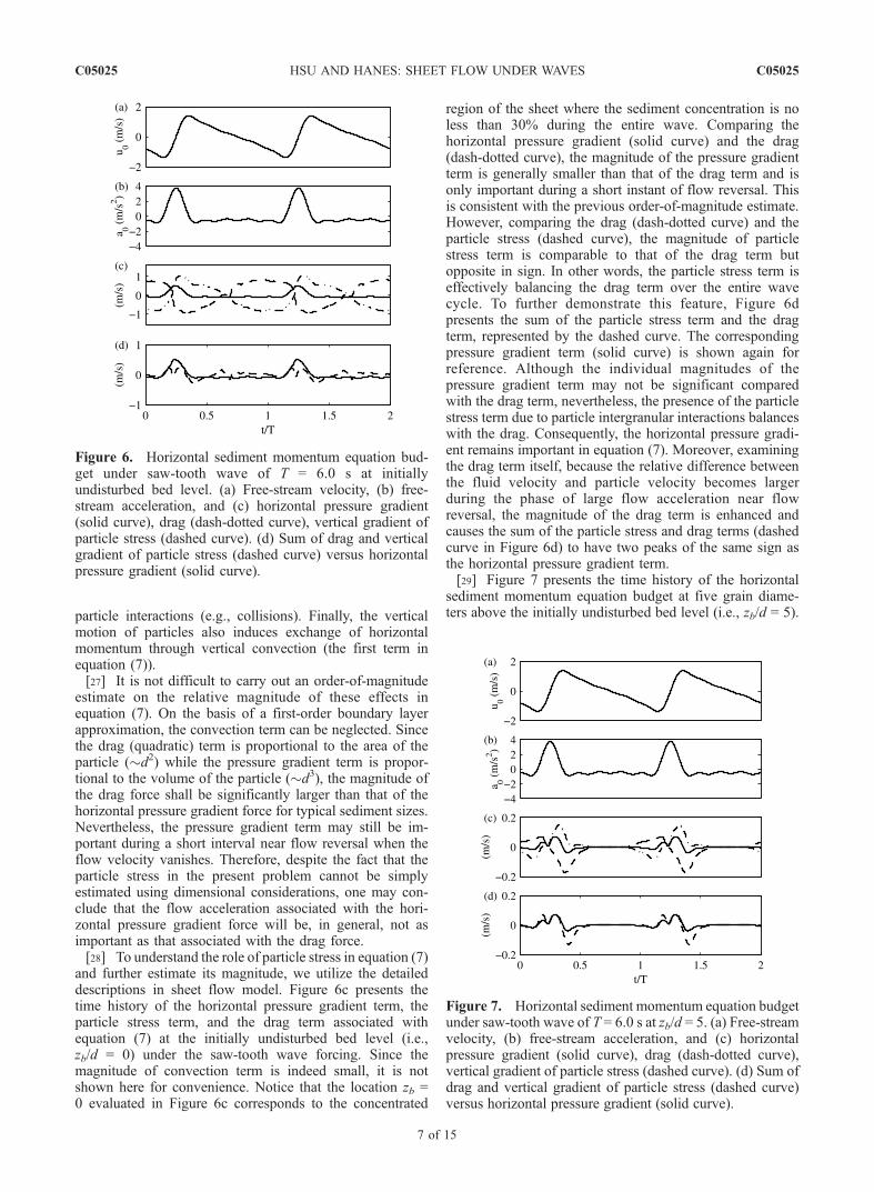
and further estimate its magnitude, we utilize the detaileddescriptions in sheet flow model. Figure 6c presents thetime history of the horizontal pressure gradient term, theparticle stress term, and the drag term associated withequation (7) at the initially undisturbed bed level (i.e.,zb/d = 0) under the saw-tooth wave forcing. Since themagnitude of convection term is indeed small, it is notshown here for convenience. Notice that the location zb =0 evaluated in Figure 6c corresponds to the concentrated

region of the sheet where the sediment concentration is noless than 30% during the entire wave. Comparing thehorizontal pressure gradient (solid curve) and the drag(dash-dotted curve), the magnitude of the pressure gradientterm is generally smaller than that of the drag term and isonly important during a short instant of flow reversal. Thisis consistent with the previous order-of-magnitude estimate.However, comparing the drag (dash-dotted curve) and theparticle stress (dashed curve), the magnitude of particlestress term is comparable to that of the drag term butopposite in sign. In other words, the particle stress term iseffectively balancing the drag term over the entire wavecycle. To further demonstrate this feature, Figure 6dpresents the sum of the particle stress term and the dragterm, represented by the dashed curve. The correspondingpressure gradient term (solid curve) is shown again forreference. Although the individual magnitudes of thepressure gradient term may not be significant comparedwith the drag term, nevertheless, the presence of the particlestress term due to particle intergranular interactions balanceswith the drag. Consequently, the horizontal pressure gradi-ent remains important in equation (7). Moreover, examiningthe drag term itself, because the relative difference betweenthe fluid velocity and particle velocity becomes largerduring the phase of large flow acceleration near flowreversal, the magnitude of the drag term is enhanced andcauses the sum of the particle stress and drag terms (dashedcurve in Figure 6d) to have two peaks of the same sign asthe horizontal pressure gradient term.[29] Figure 7 presents the time history of the horizontal

sediment momentum equation budget at five grain diame-ters above the initially undisturbed bed level (i.e., zb/d = 5).

Figure 6. Horizontal sediment momentum equation bud-get under saw-tooth wave of T = 6.0 s at initiallyundisturbed bed level. (a) Free-stream velocity, (b) free-stream acceleration, and (c) horizontal pressure gradient(solid curve), drag (dash-dotted curve), vertical gradient ofparticle stress (dashed curve). (d) Sum of drag and verticalgradient of particle stress (dashed curve) versus horizontalpressure gradient (solid curve).

Figure 7. Horizontal sediment momentum equation budgetunder saw-tooth wave of T = 6.0 s at zb/d = 5. (a) Free-streamvelocity, (b) free-stream acceleration, and (c) horizontalpressure gradient (solid curve), drag (dash-dotted curve),vertical gradient of particle stress (dashed curve). (d) Sum ofdrag and vertical gradient of particle stress (dashed curve)versus horizontal pressure gradient (solid curve).


7 of 15

C05025

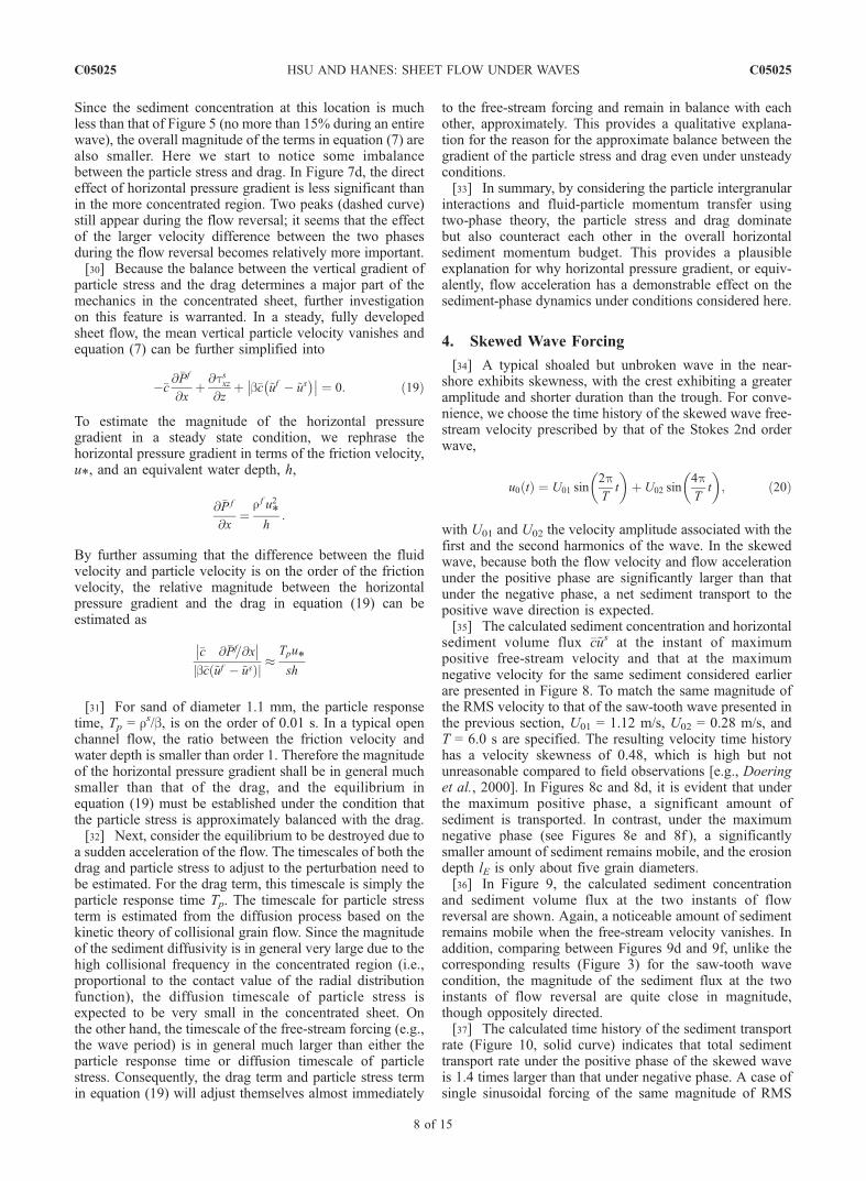
Since the sediment concentration at this location is muchless than that of Figure 5 (no more than 15% during an entirewave), the overall magnitude of the terms in equation (7) arealso smaller. Here we start to notice some imbalancebetween the particle stress and drag. In Figure 7d, the directeffect of horizontal pressure gradient is less significant thanin the more concentrated region. Two peaks (dashed curve)still appear during the flow reversal; it seems that the effectof the larger velocity difference between the two phasesduring the flow reversal becomes relatively more important.[30] Because the balance between the vertical gradient of

particle stress and the drag determines a major part of themechanics in the concentrated sheet, further investigationon this feature is warranted. In a steady, fully developedsheet flow, the mean vertical particle velocity vanishes andequation (7) can be further simplified into

��c @�Pf

@xþ @tsxz

@zþ b�c ~uf � ~us

� � ¼ 0: ð19Þ

To estimate the magnitude of the horizontal pressuregradient in a steady state condition, we rephrase thehorizontal pressure gradient in terms of the friction velocity,u*, and an equivalent water depth, h,

@�P f

@x¼

r f u2*

h:

By further assuming that the difference between the fluidvelocity and particle velocity is on the order of the frictionvelocity, the relative magnitude between the horizontalpressure gradient and the drag in equation (19) can beestimated as

�c @�Pf=@x b�c ~uf � ~usð Þj j

Tpu*sh

[31] For sand of diameter 1.1 mm, the particle responsetime, Tp = rs/b, is on the order of 0.01 s. In a typical openchannel flow, the ratio between the friction velocity andwater depth is smaller than order 1. Therefore the magnitudeof the horizontal pressure gradient shall be in general muchsmaller than that of the drag, and the equilibrium inequation (19) must be established under the condition thatthe particle stress is approximately balanced with the drag.[32] Next, consider the equilibrium to be destroyed due to

a sudden acceleration of the flow. The timescales of both thedrag and particle stress to adjust to the perturbation need tobe estimated. For the drag term, this timescale is simply theparticle response time Tp. The timescale for particle stressterm is estimated from the diffusion process based on thekinetic theory of collisional grain flow. Since the magnitudeof the sediment diffusivity is in general very large due to thehigh collisional frequency in the concentrated region (i.e.,proportional to the contact value of the radial distributionfunction), the diffusion timescale of particle stress isexpected to be very small in the concentrated sheet. Onthe other hand, the timescale of the free-stream forcing (e.g.,the wave period) is in general much larger than either theparticle response time or diffusion timescale of particlestress. Consequently, the drag term and particle stress termin equation (19) will adjust themselves almost immediately

to the free-stream forcing and remain in balance with eachother, approximately. This provides a qualitative explana-tion for the reason for the approximate balance between thegradient of the particle stress and drag even under unsteadyconditions.[33] In summary, by considering the particle intergranular

interactions and fluid-particle momentum transfer usingtwo-phase theory, the particle stress and drag dominatebut also counteract each other in the overall horizontalsediment momentum budget. This provides a plausibleexplanation for why horizontal pressure gradient, or equiv-alently, flow acceleration has a demonstrable effect on thesediment-phase dynamics under conditions considered here.

4. Skewed Wave Forcing

[34] A typical shoaled but unbroken wave in the near-shore exhibits skewness, with the crest exhibiting a greateramplitude and shorter duration than the trough. For conve-nience, we choose the time history of the skewed wave free-stream velocity prescribed by that of the Stokes 2nd orderwave,

u0 tð Þ ¼ U01 sin2pT

t

� �þ U02 sin

4pT

t

� �; ð20Þ

with U01 and U02 the velocity amplitude associated with thefirst and the second harmonics of the wave. In the skewedwave, because both the flow velocity and flow accelerationunder the positive phase are significantly larger than thatunder the negative phase, a net sediment transport to thepositive wave direction is expected.[35] The calculated sediment concentration and horizontal

sediment volume flux �c~us at the instant of maximumpositive free-stream velocity and that at the maximumnegative velocity for the same sediment considered earlierare presented in Figure 8. To match the same magnitude ofthe RMS velocity to that of the saw-tooth wave presented inthe previous section, U01 = 1.12 m/s, U02 = 0.28 m/s, andT = 6.0 s are specified. The resulting velocity time historyhas a velocity skewness of 0.48, which is high but notunreasonable compared to field observations [e.g., Doeringet al., 2000]. In Figures 8c and 8d, it is evident that underthe maximum positive phase, a significant amount ofsediment is transported. In contrast, under the maximumnegative phase (see Figures 8e and 8f ), a significantlysmaller amount of sediment remains mobile, and the erosiondepth lE is only about five grain diameters.[36] In Figure 9, the calculated sediment concentration

and sediment volume flux at the two instants of flowreversal are shown. Again, a noticeable amount of sedimentremains mobile when the free-stream velocity vanishes. Inaddition, comparing between Figures 9d and 9f, unlike thecorresponding results (Figure 3) for the saw-tooth wavecondition, the magnitude of the sediment flux at the twoinstants of flow reversal are quite close in magnitude,though oppositely directed.[37] The calculated time history of the sediment transport

rate (Figure 10, solid curve) indicates that total sedimenttransport rate under the positive phase of the skewed waveis 1.4 times larger than that under negative phase. A case ofsingle sinusoidal forcing of the same magnitude of RMS


8 of 15

C05025

velocity is also plotted here for reference. From a parame-terization point of view, under the present skewed waveshape, the net sediment transport rate may be plausiblydescribed by the free-stream flow velocity. However, on thebasis of the shape of the sediment transport rate time history,we observe that within the positive or negative phase, alarger magnitude of sediment transport tends to bulgetoward the times of larger magnitude of accelerations. Thisis especially obvious during the negative phase where themagnitude of flow velocity is relatively small for theskewed wave. For example, in Figure 10c, the peak mag-nitude of negative sediment transport occurs at about t/T =0.81, while the peak magnitude of free-stream velocity andfree-stream acceleration in the negative phase occurs at t/T =1.0 and t/T = 0.67, respectively; suggesting that sedimenttransport is influenced by flow acceleration. Despite thedetailed instantaneous variation, the overall feature in theskewed wave is that the magnitudes of free-stream velocityand corresponding acceleration are well correlated (i.e., thetimes of large velocity are close to the times of largeacceleration and vise versa.). Therefore it has been reportedthat the sediment transport rate under skewed waves can be

successfully parameterized by the third moment of free-stream velocity [e.g., Ribberink, 1998].

5. Step Acceleration Forcing

[38] Various sediment responses between two steadystates using a prescribed free stream velocity of a rampshape are now investigated to further examine the flowacceleration (or equivalently, the horizontal pressure gradi-ent) effect. First, we investigate the transient responsebetween two steady state conditions, where the mixtureboundary layer flow slowly adjusts itself from a lower free-stream velocity to a higher free-stream velocity due to aninstantaneous jump in the pressure gradient applied to forcethe system. Next, a large pressure gradient is prescribedduring a finite interval between the two steady states suchthat a constant acceleration of the free stream velocity isestablished during the transient.[39] Figure 11 illustrates the transport of coarse sand

(diameter d = 1.1 mm, specific gravity s = 2.65) duringthe transient between a low free-stream velocity of 1.02 m/sto a high free-stream velocity of 2.18 m/s due to aninstantaneous increase in the pressure gradient applied att = 0. In Figure 11a the flow has already achieved the firststeady state of free-stream velocity 1.02 m/s before t = 0 s

Figure 8. Snapshots of sediment concentration andhorizontal volume flux under Stokes second-order waveof wave period T = 6.0 s at the instant of maximum positivefree-stream velocity (inverted triangles), and maximumnegative velocity (crosses). (a) Prescribed free-streamvelocity, (b) free-stream acceleration, (c) sediment concen-tration, and (d) horizontal volume flux at the invertedtriangles; (e) sediment concentration and (f ) horizontalvolume flux at the crosses.

Figure 9. Snapshots of sediment concentration andhorizontal volume flux under Stokes second-order waveof wave period T = 6.0 s at two instants of flow reversal.(a) Prescribed free-stream velocity, (b) free-stream accelera-tion, (c) sediment concentration, and (d) horizontal volumeflux at the inverted triangles; (e) sediment concentration and(f ) horizontal volume flux at the crosses.


9 of 15

C05025

due to a lower horizontal pressure gradient. A higherhorizontal pressure gradient is imposed after t = 0 s, andthe flow adjusts itself to a second steady state of free-streamvelocity 2.18 m/s. In terms of the free-stream velocity andnondimensional total sediment transport rate (Figures 11aand 11b), it takes about 150 s for the entire flow (both thefluid and sediment phase) to adjust to the next steadystate. On the other hand, according to the erosion depth lE(Figure 11c), it only takes about 10 s for the bed to reach thelocation of the next steady state. Therefore the responsetime for bed failure and sediment entrainment is muchshorter than that of the entire boundary layer flow. Thebed responds to the variation of the external forcing quicklybecause the failure/entrainment process occurs very nearthe bed where sediment concentration is large, particleintergranular interaction dominates, and the diffusion ofmomentum becomes very efficient. On the contrary, thetotal sediment transport rate, including some transportthrough fluid turbulent suspension, must adjust to theexternal forcing according to the turbulence timescale ofthe entire flow domain.[40] Two cases for the transport of coarse sand undergo-

ing a constant acceleration between the two steady statesare presented in Figure 12. Between Figures 12b and 12c,the flow is accelerated with a constant flow accelerationof 2.37 m/s2 from the low free-stream velocity stage of1.02 m/s to the high free-stream velocity stage of 2.18 m/swithin duration of Dt = 0.49 s. Between Figures 12b and12d, the flow is accelerated between the same limitingvelocities within a duration of Dt = 1.22 s due to a lowerconstant acceleration of 0.95 m/s2. Figures 12b and 12cshow snapshots of the sediment concentration, horizontalsediment flux, and particle and fluid velocity fluctuationintensities under acceleration of 2.37 m/s2 at the beginningof the acceleration, denoted by the circle, and at the end ofthe acceleration, denoted by the asterisk, respectively. Thedashed curve in Figure 12c corresponds to the results of a

steady state case of free stream velocity of 2.18 m/s.Comparison between the dashed curve and the solid curveillustrates the effect of flow acceleration on sedimenttransport at the same free-stream velocity. From the sedi-ment flux in snapshots b-2 and c-2, it is evident that withinthe short duration of 0.49 s, more sediment is mobilized dueto higher magnitude of the flow. Specifically, comparingthe solid curve and the dashed curve in snapshot c-2, theimmobile bed location is significantly lower under largeacceleration than that of no acceleration. The flow acceler-ation considerably enhances the bed failure and mobilizesmore sediment. An interesting feature of the newly failedregion is that although it is mobile, the sediment concen-tration remains very large and its vertical distribution is veryclose to that of the steady state condition. This region couldbe identified as a highly concentrated plug flow [Sleath,1999; Foster et al., 2002]. Moreover, from snapshots c-3and c-4, noticeable particle fluctuations in the newly failedregion are observed while the fluid turbulence remainsnegligible due to high sediment concentration. Snapshotsd-1 to d-4 show the corresponding snapshots for the case oflower constant acceleration of 0.95 m/s2. On the basis ofsediment concentration and horizontal flux shown in snap-shots d-1 and d-2, the differences are less significantbetween the case of acceleration of 0.95 m/s2 and that ofno acceleration. The bed locations between these twoconditions become very close, suggesting that a flowacceleration of 0.95 m/s2 cannot cause significant bedfailure for the present particles.[41] It appears that bed failure is responsible for a major

part of the excessive sediment transport under large accel-erations. We next conduct further investigations on therelation between the flow acceleration, the bed failure,and the corresponding sediment transport rate using a seriesof step acceleration forcings. Figure 13 shows the results

Figure 10. Sediment transport under skewed forcing(solid curve) and single sinusoidal forcing (dashed curve)of wave period T = 6.0 s. (a) Prescribed free-stream velocity,(b) free-stream acceleration, and (c) nondimensional sedi-ment transport rate.

Figure 11. Transport of coarse sand during the transientbetween a low free-stream velocity of 1.02 m/s to a highfree-stream velocity of 2.18 m/s. (a) Time history of free-stream velocity, (b) nondimensional sediment transportrate, and (c) nondimensional erosion depth.


10 of 15

C05025

obtained after forcing the free-stream flow from a lowvelocity (1.02 m/s) to a high velocity (either 1.5 or2.18 m/s) at various constant accelerations. The sedimenttransport rates obtained upon just reaching the high free-stream velocity of 2.18 m/s, normalized by its steady statevalue, are plotted in the solid curve of Figure 13a. Theacceleration does not seem to noticeably enhance sedimenttransport until its magnitude is greater than about 0.25 m/s2.Within the range of acceleration between 0.25 m/s2 and1.0 m/s2, the enhanced sediment transport rate graduallyincreases but remains within 10% of that under the steadystate condition. In contrast, as the acceleration becomesgreater than about 1.0 m/s2, the corresponding sedimenttransport rate increases abruptly to about 30% more. Themajor reason for the sudden increase of sediment transportrate is revealed by examining the erosion depth lE. In thesolid curve of Figure 13b, the erosion depth is made

nondimensional by the grain diameter and plotted againstthe acceleration. Evidently, as the acceleration becomesgreater than about 1.0 m/s2, lE increases abruptly fromabout 10 grain diameters to about 15 grain diameters. Thisresults in the large sediment transport rate observed inFigure 13a. Therefore, according to the present model, thereseems to exist a critical acceleration for given sedimentparticle properties such that severe failure occurs across asignificant depth of the sediment bed.[42] Somewhat different behavior is obtained as we

evaluate the sediment transport rate at the instant wherefree-stream velocity just reaches a smaller magnitude of1.5 m/s (dotted curves of Figure 13). Since both theresults in the solid curve and dotted curve series are dueto the same magnitude of low stage free-stream velocity,evaluating at a lower high free-stream velocity also corre-sponds to a shorter duration of the constant acceleration.Nevertheless, because the calculated sediment transport ratefor each case in Figure 13a has already been normalized byits corresponding sediment transport rate in the steady state,we believe that the observed differences between the solidcurve series and the dotted curve series are due to thediffering durations of acceleration rather than due to thedifferent velocities. Specifically, when evaluated at asmaller high free-stream velocity of 1.5 m/s (dotted curve),a constant acceleration with a magnitude between 0.1 m/s2

and 2.0 m/s2 causes the corresponding sediment transportrate to be smaller than that in the steady state (i.e., qs/qs0smaller than unity). This is because when acceleration issmall, the corresponding horizontal pressure gradient is notstrong enough to cause bed failure (see the erosion depthplotted in Figure 13b). On the other hand, it takes time for

Figure 12. Snapshots of sediment concentration, sedimenthorizontal flux, and intensity of particle and fluid velocityfluctuations under two constant accelerations of 2.37 m/s2

(solid curve in Figure 12a) and 0.95 m/s2 (dash-dotted curvein Figure 12a) of step shapes. In Figures 12b–12d, the solidcurves indicate the corresponding results at the circle,asterisk, and inverted triangle shown in Figure 12a, thedashed curves indicate steady state results with the samefree-stream velocity of that at the asterisk and invertedtriangle, and the dash-dotted lines represent the location ofbed.

Figure 13. Sediment transport under prescribed stepacceleration forcing. The step has a low free-stream velocityof 1.02 m/s and high free-stream velocity of 2.18 m/s.(a) Sediment transport rate under various constant accel-eration relative to that of their steady state condition and(b) corresponding nondimensional erosion depth, evaluatedat free-stream velocity of 2.18 m/s (circles) and free-streamvelocity of 1.5 m/s (triangles).


11 of 15

C05025

the mobilized sediment to respond to the changing forcingconditions. Hence the sediment transport rate under steadystate (i.e., fully saturated) is larger than at the same freestream velocity under a constant acceleration, where a finiteduration for the development of transport is imposed, andwhere the pressure gradient is not sufficient to cause bedfailure. When acceleration becomes greater than about2.0 m/s2, the effect of bed failure dominates and thecorresponding sediment transport increases.[43] Notice that the erosion depth and the corresponding

sediment transport rate begin to decrease as the accelera-tion becomes greater than about 3.0 m/s2. Because anacceleration of 3.0 m/s2 for these cases corresponds to aduration of acceleration of only Dt = 0.39 s, the observeddecrease of the erosion depth and sediment transport rateagain suggests a minimum development timescale offailure for the sediment bed in response to the changingflow.[44] Using the step forcing, we have demonstrated that

the bed failure is closely related to flow acceleration/horizontal pressure gradient. However, it appears to requiresome time for both sediment transport and turbulent flow toadjust to the changing forcing conditions, and it alsorequires some shorter amount of time for the bed tocompletely fail or yield. We will refer to these two time-scales as the saturation timescale and yield timescale,respectively. Because large acceleration often suggests ashorter duration of forcing, flow acceleration does notalways enhance sediment transport. We believe that forsmall accelerations where the bed failure is not significant,the acceleration may cause a decrease in the sedimenttransport rate if the duration of forcing does not exceedthe saturation timescale. On the contrary, when accelerationis large enough to approach or exceed the critical acceler-ation for bed failure, enhancing acceleration results in moresevere failure and larger sediment transport. However, evenfor large accelerations, if the duration of forcing is shorterthan the yield timescale, enhancing acceleration may againresult in smaller sediment transport rate. Finally, we believethat the saturation and yield timescales are also functions ofthe magnitude of the flow velocity, the flow acceleration,and the fluid and sediment properties. Further systematicanalysis on these issues and critical experiments are clearlymotivated.[45] One of the key features of unsteady sheet flows is

that the amount of mobilized sediment and the location ofthe bed change with time. Bagnold [1956] argues that forsteady flows the immersed weight of the sheet flow layer isrelated to the bed shear stress through a dynamic Coulombyield criterion. If for some reason the bed shear stressincreases slowly, then in the quasi-steady Bagnold para-digm, successive layers of stationary grains would beentrained into the flow until the newly increased immersedweight balanced the increase in the bed shear stress.However, results presented earlier also suggest that undervery high accelerations the bed undergoes a sudden failure,analogous to the episodic avalanching of sand that is piledsteeper than the critical angle of repose.[46] Madsen [1974] performs an analysis on the momen-

tary internal failure of sand bed under waves. He demon-strates that momentary bed failure under waves is morelikely to be initiated by shear failure due to significant

horizontal pressure gradient and less likely to be initiated bythe vertical flow in the porous bed. Moreover, Madsenintroduces a simple formula, based on the properties ofthe sand bed, to calculate the critical horizontal pressuregradient for momentary shear failure. On the basis of thetwo-phase equations, the horizontal momentum equation forthe sediment-fluid mixture can be obtained by combiningthe horizontal momentum equation of the fluid and sedi-ment phase. At the stationary bed, because all the particlemotion vanishes and the fluid horizontal velocity can bealso neglected for simplicity, a simplified mixture equation,similar to that used by Madsen [1974], becomes

�r f@u0 tð Þ@t

¼@ t f

xz þ tsxz� �

@z; at zb ¼ �lE: ð21Þ

Note that the horizontal pressure gradient term has beenreplaced by the free-stream acceleration. Equation (21)indicates that the gradient of total shear stress at bed mustrespond to the given flow acceleration, a surrogate forhorizontal pressure gradient.[47] To calculated the right-hand side of equation (21),

Madsen [1974] further adopts the quasi-steady Bagnoldparadigm [Bagnold, 1956], in which the gradient of totalshear stress at bed is related to the normal stress throughCoulomb failure and calculated by the immersed weight ofsediment in fluid,

@ tfxz þ tsxz� �

@z¼ rs � rf

� ��cjgj tanf; at zb ¼ �lE: ð22Þ

Combining equations (21) and (22), and applying typicalvalues for sediment density, concentration, and internalfriction angle, this analysis suggests that an acceleration ofapproximately 0.4 jgj is enough to cause catastrophic failurewithin the bed. Strictly speaking, because the closurepresented in equation (22) is only valid in the fullydeveloped steady state condition, the quasi-steady approachadopted by Madsen [1974] may be too simple to evaluatebed failure under highly unsteady conditions. The consti-tutive relations and closures used in the present two-phasemodel embody substantially more physics than Bagnold’sdescriptions. On the basis of numerical experiments ofvarious step forcing using the sheet flow model (Figure 13),we also demonstrate that when the flow acceleration/horizontal pressure gradient exceeds a critical value, rapidinternal bed failure occurs.[48] Sleath [1999] presents another analysis of the con-

dition for the so-called ‘‘plug’’ formation motivated by hismeasured laboratory data [Dick and Sleath, 1991; ZalaFlores and Sleath, 1998]. We note here that the ‘‘plug ’’that was described by Sleath [1999] is essentially the sameas the bed failure described by Madsen [1974] and thepresent paper. On the basis of a somewhat more complicatedquasi-steady analysis than Madsen [1974], Sleath [1999]introduces another parameter S = U0w/(s � 1) g for the plugformation with w the radial frequency. On the basis of hisanalysis and the measured data using acrylic particles (d =0.7 mm, s = 1.14), he suggests that the plug may form whenS is greater than a critical value (about 0.37 to 0.76). SinceU0w defined in S is equivalent to an averaged accelerationunder sinusoidal wave forcing, a critical acceleration similar


12 of 15

C05025

to that of Madsen [1974] and the present paper is alsoreported by Sleath [1999].[49] All these models indicate the existence of critical

acceleration/horizontal pressure gradient for bed failure,although our simulation results suggest failure occurs inthe dynamic system at a somewhat lower threshold accel-eration than that suggested by the quasi-static analysis.Notice that Sleath [1999] also observes that the criticalvalue for S also depends on the degree of compaction of thesediment. On the basis of our numerical experiments, ourmodel also indicates that the bed failure or the erosion depthunder unsteady forcing depends on the compaction of thebed.[50] In addition to laboratory experiments, recent field

observations of Foster et al. [2002] also suggested theoccurrence of plug flow during flow reversal. Because thebed failure can be a direct consequence of the large flowacceleration/horizontal pressure gradient, further measure-ments toward a better understanding of bed failure arenecessary [e.g., Cox et al. 1991].

6. Toward Parameterization

[51] On the basis of the two-phase model, we demon-strate that whether the net sediment transport rate can beplausibly parameterized by the flow velocity depends onthe wave shape. In particular, it is insufficient to simplyuse the instantaneous flow velocity to calculate thecorresponding time-dependent sediment transport rate ina quasi-steady sense. This results from several mecha-nisms, such as the closures of fluid and sediment stresses,the effect of pressure gradient on the particles, and bedfailure, that are not incorporated in the quasi-steady

parameterization procedures. Hence our next objective isto explore a new calculation procedure for the sedimenttransport rate that incorporates essential unsteady effects.[52] The nondimensional bed shear stress, usually called

the Shields parameter,

Q ¼ tbrs � rfð Þgd ; ð23Þ

is perhaps the most well-accepted parameter in characteriz-ing sediment transport processes [e.g., Ribberink, 1998]. Wepoint out here that the location of the bed shear stress isclearly defined for fixed beds, but that for unsteady sheetflows the vertical location of the stationary bed changes intime. In addition, the fluid and granular phase shear stressesvary with vertical position and time. Since the closures ofboth the fluid and particle stresses have been incorporated inthe model, the total shear stress at any level within the sheet,including the bed shear stress, becomes part of the solutionof the model. Here the term ‘‘bed shear stress’’ is used toindicate the instantaneous total shear stress at the uppermostlevel of the stationary bed. Figure 14c shows the calculatedtime history of the nondimensional bed shear stress, whichwe shall refer to as q(t), the generalized Shields parameter,due to the saw-tooth forcing considered earlier. Notice thatunlike the time history of free-stream velocity shown inFigure 14a, the time history of q(t) is not symmetric withrespect to the positive and negative phase. Therefore aformula that calculates q(t) solely based on the free-streamvelocity is inappropriate. Moreover, since the shape of q(t)in Figure 14c is similar to the time history of the sedimenttransport rate presented in Figure 14c, we are motivated toestimate the sediment transport rate by substituting thegeneralized Shields parameter, q(t), into the Meyer-PeterMuller formula,

� tð Þ ¼ 8 q tð Þ � 0:05½ �3=2: ð24Þ

The resulting nondimensional sediment transport rate(solid curve in Figure 14d) closely resembles the directcalculations from the sheet flow model (dashed curve).Therefore the present sheet flow model indicates that it is,at least qualitatively, reasonable to apply a steady stateformula in a quasi-steady manner to an unsteadycondition as long as the corresponding bed shear stresscan be accurately estimated.[53] Owing to improved computational power, phase-

resolving models for surfzone hydrodynamics and sedimenttransport have become popular in recent years [e.g.,Wei andKirby, 1995; Lin and Liu, 1998]. Therefore it would beextremely useful to develop a reliable and efficient calcu-lation procedure for instantaneous sediment transport ratethat incorporates essential unsteady effects. On the basis ofthe two-phase model, we believe that given the instanta-neous bed shear stress, a quasi-steady approach may beapplied to estimate the instantaneous sediment transportrate. However, such calculation procedure must rely onaccurate prediction on instantaneous bed shear stress whichmay not be parameterized solely by the flow velocity quasi-steadily.[54] For a predictive nearshore morphological model, a

more efficient approach to calculate the bed shear stress

Figure 14. Sediment transport under saw-tooth wave ofwave period T = 6.0 s. (a) Prescribed free-stream velocity,(b) free-stream acceleration, and (c) nondimensional bedshear stress. (d) Nondimensional sediment transport rateusing calculated nondimensional bed shear stress andMeyer-Peter Muller formula (solid curve) and two-phasesheet flow model (dashed curve).


13 of 15

C05025

than the present two-phase model is necessary. Nielsen[1992] and Nielsen and Callaghan [2003] propose aformula to calculate the instantaneous bed shear stressthat explicitly incorporates flow velocity and acceleration.However, the development of a more physical-based,yet efficient calculation procedure for instantaneous bedshear stress is nontrivial [e.g., Grant and Madsen, 1979;Trowbridge and Madsen, 1984]. Evidently, in a waveboundary layer flow, the near-bed flow velocity would becompletely in phase with the free-stream velocity if the flowwere inviscid. In other words, an accurate prediction of bedshear stress must rely on reasonable closure on fluid andsediment stresses. For this, whether we can cost-effectivelyparameterize (or simplify) the vertical distribution of thefluid turbulence and particle intergranular interactionsacross the wave boundary layer becomes crucial andrequires future work.

7. Conclusion

[55] Using a recently developed two-phase model,we examine in detail the effects of wave shape onsediment transport. We find that for certain wave shapes,time-dependent sediment transport cannot be completelyparameterized by the instantaneous free-stream velocity.Examinations of the sheet flow response to flow forcingtypical of asymmetric and skewed waves indicate a netsediment transport in the direction of wave propagation.[56] Using a closure of particle intergranular stress based

on the kinetic theory of granular flow in the two-phaseequations, we examine the role of the particle collisionalstress in the sediment momentum budget. The particlecollisional stress tends to effectively balance the dragforce in the sediment horizontal budget and thus enhancethe relative effect of horizontal pressure gradient on thesediment dynamics. Moreover, numerical experimentsindicate that catastrophic internal bed failure is a directconsequence of large horizontal pressure gradient (or largeflow acceleration).[57] Using the sheet flow model, we demonstrate that

a power law, which can be as simple as the Meyer-Peter Muller formula, can predict the sediment transportreasonably well as long as accurate description for thecorresponding instantaneous bed shear stress can beobtained. We believe these results will provide new guide-lines toward an improved parameterization for sedimenttransport rate under unsteady conditions.[58] Finally, we note here that all the simulations pre-

sented in this work were for coarse sand with a diameter of1.1 mm. For such coarse sediment, collisions betweengrains are dominated by the grains’ inertia, the fluid playsa minor role, and the kinetic theory for granular flowappropriately captures the dominant momentum and energypathways. More typical beach sand, of diameter 0.2 mm forexample, may behave differently due to the relativelygreater influence of the interstitial fluid upon the grain-to-grain interactions. We believe one of the most importantextensions of this and previous work would be to modelsediment transport of fine and medium sands using the two-phase approach with the closure of particle stresses basedon particle fluctuation energy and concentrated viscoussuspension models.

[59] Acknowledgments. We gratefully acknowledge the financialsupports of the National Ocean Partnership Program and the Departmentof Civil and Environmental Engineering, University of Delaware. Numer-ous discussions with James Jenkins and Philip Liu during the developmentof the sheet flow model are appreciated. We also wish to thank James Kirby,John Warner, Jon Warrick, and Fernanda Hoefel for their useful commentson earlier versions of this manuscript.

ReferencesAsano, T. (1995), Sediment transport under sheet-flow conditions,J. Waterw. Port Coast. Ocean Eng., 121(5), 1–8.

Bagnold, R. A. (1956), The flow of cohesionless grains in fluid, Philos.Trans. R. Soc. London, Ser. A, 249(964), 235–297.

Bailard, J. (1981), An energetic total load sediment transport model for aplane sloping beach, J. Geophys. Res., 86, 10,938–10,954.

Bocquet, L., W. Losert, D. Schalk, T. C. Lubensky, and J. P. Gollub (2002),Granular shear flow dynamics and forces: Experiment and continuumtheory, Phys. Rev. E, 65(1), 011307.

Butt, T., and P. Russell (1999), Suspended sediment transport mechanism inhigh-energy swash, Mar. Geol., 161, 361–375.

Cox, D. T., N. Kobayashi, and M. Hajime (1991), Effect of fluid accelera-tion on sediment transport in surf zone, Coastal Sed., 91, 447–461.

Dick, J. E., and J. F. A. Sleath (1991), Velocities and concentrations inoscillatory flow over beds of sediment, J. Fluid Mech., 233, 165–196.

Doering, J. C., B. Elfrink, D. M. Hanes, and G. Ruessink (2000),Parameterization of velocity skewness under waves and its effect oncross-shore sediment transport, paper presented at 27th Coastal Engineer-ing Conference, Am. Soc. of Civ. Eng., Reston, Va.

Dohmen-Janssen, C. M., and D. M. Hanes (2002), Sheet flow dynamicsunder monochromatic nonbreaking waves, J. Geophys. Res., 107(C10),3149, doi:1029/2001JC001045.

Drake, T. G., and J. Calantoni (2001), Discrete particle model for sheet flowsediment transport in the nearshore, J. Geophys. Res., 106(C9), 19,859–19,868.

Drew, D. A. (1976), Production and dissipation of energy in the turbulentflow of a particle-fluid mixture, with some results on drag reduction,J. Appl. Mech., 43, 543–547.

Elgar, S., and R. T. Guza (1985), Observations of bispectra of shoalingsurface gravity waves, J. Fluid Mech., 161, 425–448.

Elgar, S., E. L. Gallagher, and R. T. Guza (2001), Nearshore sandbarmigration, J, Geophy. Res., 106(C6), 11,623–11,627.

Elghobashi, S. E., and T. W. Abou-Arab (1983), A two-equation turbulencemodel for two-phase flows, Phys. Fluids, 26(4), 931–938.

Foster, D. L., R. A. Holman, and A. J. Bowen (2002), Field evidencefor plug flow, Eos Trans. AGU, 83(47), Fall Meet. Suppl., AbstractOS72C-02.

Gallagher, E. L., S. Elgar, and R. T. Guza (1998), Observations of sand barevolution on a natural beach, J. Geophys. Res., 103(C2), 3203–3215.

Grant, W. D., and O. S. Madsen (1979), Combined wave and currentinteraction with a rough bottom, J. Geophys. Res., 84(C4), 1797–1808.

Hanes, D. M., and D. A. Huntley (1986), Continuous measurements ofsuspended sand concentration in a wave dominated nearshore environ-ment, Cont. Shelf Res., 6, 585–596.

Hanes, D. M., and D. L. Inman (1985a), Observations of rapidly flowinggranular-fluid materials, J. Fluid Mech., 150, 357–380.

Hanes, D. M., and D. L. Inman (1985b), Experimental evaluation of adynamic yield criterion f or gr anular-fluid f low, J. Geophys. Res.,90(B5), 3670–3674.

Ho efe l , F., and S. E lg ar (200 3), Wave-in duc ed s edim ent t rans por t andsandbar migration, Science, 299 , 1885 – 1887.

Hsu, T.-J., J. T. Jenkins, and P. L.-F. Liu (2003), On two-phase sediment trans-port: Dilute flow, J. Geophys. Res., 108(C3), 3057, doi:10.1029/2001JC001276 .

Hsu, T.-J., J. T. Jenkins, and P. L.-F. Liu (2004), On two-phase sedimenttransport: Sheet flow of massive particles, Proc. R. Soc. London, Ser. A,460(2048), doi:10.1098/rspa.2003.1273.

Jenkins, J. T., and D. M. Hanes (1998), Collisional sheet flows of sedimentdriven by turbulent fluid, J. Fluid Mech., 370, 29–52.

Jenkins, J. T., and S. B. Savage (1983), A theory for the rapid flow ofidentical, smooth, nearly elastic particles, J. Fluid Mech., 370, 29–52.

Jenkins, J. T., P. A. Cundall, and I. Ishibashi (1989), Micromechanicsmodeling of granular material, in Powders and Grains, edited byJ. Biarez and R. Gourves, pp. 257–264, A. A. Balkema, Brookfield, Vt.

King, D. B. (1990), Studies in oscillatory flow bed load sediment transport,Ph.D. thesis, Univ. of Calif., San Diego.

Lin, P., and P. L.-F. Liu (1998), A numerical study of breaking waves in thesurf zone, J. Fluid Mech., 359, 239–264.

Madsen, O. S. (1974), Stability of a sand bed under breaking waves, paperpresented at 14th Coastal Engineering Conference, Am. Soc. of Civ.Eng., Reston, Va.


14 of 15

C05025

Masselink, G., and M. G. Hughes (1998), Field investigation of sedimenttransport in the swash zone, Cont. Shelf Res., 18, 1179–1199.

Nielsen, P. (1992), Coastal Bottom Boundary Layers and Sediment Trans-port, World Sci., River Edge, N. J.

Nielsen, P. (2002), Shear stress and sediment transport calculations forswash zone modeling, Coastal Eng., 45, 53–60.

Nielsen, P., and D. P. Callaghan (2003), Shear stress and sediment transportcalculations for sheet flow under waves, Coastal Eng., 47, 347–354.

Puleo, J. A., K. T. Holland, N. G. Plant, D. N. Slinn, and D. M. Hanes(2003), Fluid acceleration effects on suspended sediment transport in theswash zone, J. Geophys. Res., 108(C11), 3350, doi:10.1029/2003JC001943.

Ribberink, J. S. (1998), Bed-load transport for steady flows and unsteadyoscillatory flows, Coastal Eng., 34, 59–82.

Richardson, J. F., and W. N. Zaki (1954), Sedimentation and fluidization:1, Trans. Inst. Chem. Eng., 32, 35–53.

Sleath, J. F. A. (1999), Conditions for plug formation in oscillatory flow,Cont. Shelf Res., 19, 1643–1664.

Sumer, B. M., A. Kozakiewicz, J. Fredsøe, and R. Deigaard (1996),Velocity and concentration profiles in sheet-flow layer of movable bed,J. Hydrol. Eng., 122(10), 549–558.

Torquato, S. (1995), Nearest-neighbor statistics for packings of hardspheres and disks, Phys. Rev. E, 51, 3170–3182.

Trowbridge, J., and O. S. Madsen (1984), Turbulent wave boundary layers:2. Second-order theory and mass transport, J. Geophys. Res., 89(C5),7999–8007.

Wei, G., and J. T. Kirby (1995), A time-dependent numerical code forextended Boussinesq equations, J. Waterw. Port Coastal Ocean Eng.,121, 251–261.

Young, J., and A. Leeming (1997), A theory of particle deposition inturbulent pipe flow, J. Fluid Mech., 340, 129–159.

Zala Flores, N., and J. F. A. Sleath (1998), Mobile layer in oscillatory sheetflow, J. Geophys. Res., 103(C6), 12,783–12,793.

��D. M. Hanes, Western Coastal and Marine Geology, U.S. Geological

Survey Pacific Science Center, 400 Natural Bridges Drive, Santa Cruz, CA95060, USA. ([email protected])T.-J. Hsu, Woods Hole Oceanographic Institution, Applied Ocean

Physics and Engineering Department, MS 11, Woods Hole, MA 02543,USA. ([email protected])


15 of 15

C05025

effects of wave shape on sheet flow sediment transport of wave shape on sheet flow sediment...

Documents