effects of topography on assessing wind farm impacts using

Effects of Topography on AssessingWind Farm Impacts UsingMODIS DataLiming Zhou*

Department of Atmospheric and Environmental Sciences, University at Albany,State University of New York, Albany, New York

Yuhong Tian

IMSG, NOAA/NESDIS/STAR, College Park, Maryland

Haishan Chen

Key Laboratory of Meteorological Disaster, Ministry of Education, Nanjing Universityof Information Science and Technology, Nanjing, China

Yongjiu Dai

School of Geography, Beijing Normal University, Beijing, China

Ronald A. Harris

Department of Atmospheric and Environmental Sciences, University at Albany,State University of New York, Albany, New York

Received 17 December 2012; accepted 27 June 2013

*Corresponding author address: Liming Zhou, Department of Atmospheric and Environ-mental Sciences, University at Albany, State University of New York, 1400 Washington Avenue,Albany, NY 12222.

E-mail address: [email protected]

Earth Interactions d Volume 17 (2013) d Paper No. 13 d

DOI: 10.1175/2012EI000510.1

Copyright � 2013, Paper 17-013; 45117 words, 6 Figures, 0 Animations, 1 Tables.http://EarthInteractions.org

ABSTRACT: This paper uses the empirical orthogonal function (EOF) anal-ysis to decompose satellite-derived nighttime land surface temperature (LST)for the period of 2003–11 into spatial patterns of different scales and thus toidentify whether (i) there is a pattern of LST change associated with the de-velopment of wind farms and (ii) the warming effect over wind farms reportedpreviously is an artifact of varied surface topography. Spatial pattern and timeseries analysis methods are also used to supplement and compare with the EOFresults. Two equal-sized regions with similar topography in west-central Texasare chosen to represent the wind farm region (WFR) and nonwind farm region(NWFR), respectively. Results indicate that the nighttime warming effect seenin the first mode (EOF1) in WFR very likely represents the wind farm impactsdue to its spatial coupling with the wind turbines, which are generally built ontopographic high ground. The time series associated with the EOF1 mode inWFR also shows a persistent upward trend over wind farms from 2003 to 2011,corresponding to the increase of operating wind turbines with time. Also, thewind farm pixels show a warming effect that differs statistically significantlyfrom their upwind high-elevation pixels and their downwind nonwind farmpixels at similar elevations, and this warming effect decreases with elevation. Incontrast, NWFR shows a decrease in LSTwith increasing surface elevation andno warming effects over high-elevation ridges, indicating that the presence ofwind farms in WFR has changed the LST–elevation relationship shown inNWFR. The elevation impacts on Moderate Resolution Imaging Spectroradi-ometer (MODIS) LST, if any, are much smaller and statistically insignificantthan the strong and persistent signal of wind farm impacts. These results pro-vide further observational evidence of the warming effect of wind farms re-ported previously.

KEYWORDS: Wind farm impact; Empirical orthogonal function; Landsurface temperature

1. IntroductionClimate change is one of the most serious environmental issues of our time.

Wind power as an alternative clean energy source to fossil fuels supports envi-ronmental sustainability and possibly provides part of the solution to our energysecurity problem (Pacala and Socolow 2004; NRC 2007; Pryor and Barthelmie2011). The use of wind power in the United States and other countries like China,Germany, Spain, and India has experienced continuous growth in recent years.Wind energy currently amounts to ;3% of U.S. electricity generation (AWEA2012; U.S. DOE 2012) and could supply up to 20% of the total U.S. electricity by2030 (U.S. DOE 2008). To generate this substantial amount of energy, wind farmswould have to install a huge number of wind turbines over a continental-scale area(Wang and Prinn 2010; Fiedler and Bukovsky 2011).

Wind power depends on weather and climate, and wind farms, if large enough,might also modify the weather and climate, at least in their immediate vicinity.While converting wind’s kinetic energy into electrical power, wind turbines modifysurface fluxes of heat, momentum, moisture, and CO2 exchanges in the atmo-spheric boundary layer (ABL) (Rajewski et al. 2013) and enhance turbulence intheir rotor wakes, thus increasing the vertical mixing within ABL (Baidya Roy andTraiteur 2010). The net effect should be small and local for a limited numberof wind turbines but may become noticeable if hundreds or thousands of wind


turbines are installed over a particular region. During the past few years a growingnumber of numerical simulations using global and regional models with hypo-thetical wind farms have generally agreed that wind farms can affect local toregional weather and climate (e.g., Keith et al. 2004; Kirk-Davidoff and Keith2008; Wang and Prinn 2010; Fiedler and Bukovsky 2011; Fitch et al. 2013).However, these studies are primarily in the model domain, with limitations anduncertainties due to the use of simple subgrid-scale wind turbine parameteriza-tions and the lack of observations for validation.

Increasing scientific and public interests in assessing environmental conse-quences of wind farms highlight the need to understand the detailed processes ofobserved meteorological fields at wind farm/turbine scales (Rajewski et al. 2013)and to develop the modeling capability to characterize wind turbine–atmosphereinteractions in numerical models. Doing so requires high-resolution observations(in both space and time) over operating wind farms. However, the general structureand functioning of wind farms, wind turbine parameters, and meteorological ob-servations within wind farms are proprietary and thus not available to the public.Furthermore, most wind farms are not within the synoptic weather observationalnetwork, which makes the use of conventional meteorological data challenging.

The availability of high-resolution remote sensing data provides an observa-tional approach to detect, quantify, and attribute wind farm impacts with spatialdetail. Satellite-derived land surface temperature (LST) measures the temperatureof Earth’s surface thermal emission. LST has a stronger day–night variation thansurface air temperatures from daily weather reports and thus is more sensitive tochanges in surface conditions (Jin and Dickinson 2002; Imhoff et al. 2010). Zhouet al. (Zhou et al. 2012) find a nighttime warming effect over large wind farms inwest-central Texas using winter and summer mean LSTs derived from the Mod-erate Resolution Imaging Spectroradiometer (MODIS). Zhou et al. (Zhou et al.2013) provides further observational evidence of this warming effect by analyzingdiurnal and seasonal variations of MODIS LST anomalies with more observationsunder different quality controls.

The wind turbines in the study region of Zhou et al. (Zhou et al. 2012; Zhou et al.2013) are generally built on mountain ridges that overlap with the reported warmingeffect. This raises a critical question of whether this warming effect is an artifactof topography. Mountains affect climate by changing the patterns of temperature,wind circulation, and precipitation (Minder et al. 2010). While variations in ele-vation, terrain slope, and aspect angles can interact with satellite viewing geometryto cause biases in retrieved LSTs (Lipton and Ward 1997; Liu et al. 2009), only theelevation effect and zenith angle changes were corrected in the routine retrieval inthe MODIS LSTs (Wan and Li 1997; Wan 2006). Hence, some residual topo-graphic effects may still exist in the MODIS LSTs. Furthermore, using satellitedata to detect and quantify wind farm impacts is still in the exploratory stage. LSTvariations over an operational wind farm contain not only the local wind turbineeffect but also the variability controlled by surface properties (Zhang et al. 2010;Imhoff et al. 2010) and large-scale meteorological conditions (Zhou et al. 2012).Separating the local versus regional- to large-scale variability of the MODIS LSTsis crucial to uncovering the wind farm effect. To identify and quantify the windfarm impacts, Zhou et al. (Zhou et al. 2012) simply use the areal mean LST dif-ferences (i) between two periods and (ii) between wind farm pixels and nearby


nonwind farm pixels, while the topographic effect on LST has to be assessed atthe pixel level. In addition, LSTs also contain uncertainties due to residual at-mospheric effects and errors from observations and retrievals (Wan 2006).Therefore, considering the significant implications of this finding, it is necessary touse other approaches to verify that the reported warming effect over wind farms isnot an artifact of varied surface topography.

Here we use an empirical orthogonal function (EOF) analysis to explore thestructure of LST variability fromMODIS, identify the spatial patterns of variability(EOF modes) and their time variations (EOF time series), and give a measure of the‘‘importance’’ of each pattern. We choose EOF analysis for its potential to evaluatethe spatial pattern of LST changes. EOF determines a set of orthogonal functionsthat characterizes the covariability of time series for a set of grid points. The degreeof spatial covariability may help uncover underlying processes of changes detectedby using satellite data (e.g., Zhou et al. 2001). Pixels with strong spatial covariancereflect similar year-to-year LST changes. If changes in LST are due to variations ofsurface topography, we would expect to see a high degree of spatial covariabilityover regions with similar elevations. If LST variations are dominated by a ran-domly distributed (in space) effect such as data noise, we would expect pixels toshow differences in LST variations that lack spatial coherence. If changes in LSTare due to the presence of operational wind turbines, we would expect a highdegree of spatial covariability over pixels with wind turbines. However, we realizethat MODIS time series might be too short to draw any definite conclusions basedon EOF analysis alone. Therefore, the approaches of spatial pattern and time seriesanalysis in Zhou et al. (Zhou et al. 2012; Zhou et al. 2013) are also used to sup-plement and compare with the EOF results but with an emphasis on the topographiceffect at pixel level, which was not done previously.

The objective of this paper is threefold. First, it aims to find whether the EOFapproach can decompose the LSTs into spatial patterns of different scales and thushelp to identify whether there is a pattern associated with the development of windfarms. Second, it serves as a detailed analysis to examine whether the warmingeffect over wind farms reported by Zhou et al. (Zhou et al. 2012) is primarily due tovaried topography at pixel level. Third, it explores EOF as a different approach toverify whether the results of Zhou et al. (Zhou et al. 2012) are robust.

2. Data and methods

2.1. Study region

We choose two equal-sized regions in west-central Texas that are close to eachother and share similar topography in terms of elevation, slope, and orientation ofterrain features, one with wind farms and the other without wind farms, which arereferred to as the wind farm region (WFR) and the nonwind farm region (NWFR),respectively. The WFR (32.18–32.98N, 1018–99.88W; Figure 1) had 2358 windturbines installed by 2011, with;90% completed by 2008. The wind turbines areidentified geographically based on the database of the Federal Aviation Admin-istration (FAA) (Zhou et al. 2012) and verified via Google Earth (Zhou et al.2013). As there are several other wind farms near WFR, it is impossible to find anNWFR without any wind turbines. Instead, we identify a region (30.58–31.38N,


100.98–99.78W; Figure 1) to the south of WFR as NWFR that has 99 wind tur-bines built in and after 2009. The presence of these 99 wind turbines is expectedto have a very limited impact on LST in NWFR because (i) the total number ofwind turbines is small and (ii) most of the wind turbines are likely operating onlyin the last 1–2 years of the study period. WFR consists of four of the world’slargest wind farms and has the highest concentration of wind turbines in west-central Texas. Particularly, the majority of the wind turbines were built between2005 and 2008, which makes it possible to use ;10 years of MODIS data. Forother wind farms near WFR, most wind turbines were installed recently, making ittoo short to investigate their impacts on LSTs.

2.2. Data processing

The collection-5 MODIS 8-day-average 1-km LST images are aggregated spa-tially and temporally into seasonal [December–February (DJF) and June–August(JJA)] and annual (ANN) means and anomalies at 0.018 resolution for the period

Figure 1. Elevation (m) map of west-central Texas that contains WFR (upper box)and NWFR (lower box) at spatial resolution of 30 arc-s (~1.0 km). Clusterpixels in black with a plus symbol are wind turbines: 2358 in WFR (32.18–32.98N, 1018–99.88W) and 99 (the inner rectangle) in NWFR (30.58–31.38N,100.98–99.78W). The pixels in black with a plus symbol outside the innerrectangle in NWFR are AWFPs.


of 2003–11, as done by Zhou et al. (Zhou et al. 2013). The MODIS LST data havebeen proven to be of high quality in a variety of studies (Wan 2006). The LSTimages consist of four acquisitions (;1030 and;1330 local solar time at daytimeand ;2230 and ;0130 local solar time at nighttime) and have quality assurance(QA) values for each image. For simplicity, we will not consider daytime LSTs andQA information of MODIS LSTs in the present analysis because the impacts ofwind farms on LST (i) are too small to be detected at daytime and (ii) differ onlyslightly under different QA controls (Zhou et al. 2013). We also combine the twoLSTs at;2230 and;0130 local solar time to produce one average nighttime LSTto reduce data uncertainties/noise and only consider the MODIS LSTs with a wholeyear of data (Zhou et al. 2012). Furthermore, we show primarily the results of JJAat nighttime when the wind farm impacts are largest but also supplement ouranalysis with some results in DJF and ANN. DJF represents the season with theleast wind farm impact. In total, there are nine images (from 2003 to 2011) forevery season (DJF, JJA, and ANN) in each study region (WFR and NWFR) andeach image has 9600 pixels (120 columns 3 80 lines).

The wind turbines in WFR are generally built on mountain ridges, with anaverage elevation of 749.1 6 21.4m based on the wind turbine site elevation dataof FAA (Figure 1). The 99 wind turbines in NWFR are also located in mountainridges (Figure 1). The global 30 arc-s elevation dataset (GTOPO30) global digitalelevation map with a horizontal grid spacing of 30 arc-s (;1.0 km) was down-loaded online (from http://eros.usgs.gov/#/Find_Data/Products_and_Data_Available/gtopo30_info). We reproject the elevation data into the 0.018 pixels as done for theMODIS LSTs. In total, there are 890 pixels with at least one wind turbine, referredto as wind farm pixels (WFPs), in WFR and 51 WFPs in NWFR at the 0.018resolution (Figure 1). We plan to compare the LST changes of WFPs betweenWFR and NWFR, but the sample size of the latter is too small and so we artifi-cially designate some pixels as ‘‘wind farms’’ in NWFR following the elevationhistogram of real wind farms in WFR (Figure 2a). Among the 9600 pixels, wechoose 2276 with an elevation greater than 712m (.76th percentile) in WFR and1920 with an elevation greater than 731m (.80th percentile) in NWFR as high-elevation pixels. These pixels generally represent the site elevations of wind tur-bines as 734 out of 890WFPs (i.e., 82.5%) belong to the 2276 high-elevation pixelsin WFR. Note that the wind turbines in WFR were mostly built over ridges whoseelevations are higher than their surroundings across the study region, not only overthe highest ridge pixels in the northwestern WFR (Figure 1). The 76th and 80thpercentile thresholds are chosen so that two groups of pixels defined in the nextparagraph will have a similar number of pixels and a similar elevation distributionas the real wind farm pixels.

To resemble the real wind turbines over high elevations, we randomly choose849 pixels from the 1920 high-elevation pixels in NWFR. To differentiate thesepixels from real WFPs, we refer to these 849 pixels plus 51 WFPs (in total890 pixels) as artificial wind farm pixels (AWFPs) in NWFR (Figure 1). These849 pixels are chosen randomly instead from a particular area because it is difficultto justify the choice of one area over another. The presence of wind turbines willhave an effect on their downwind pixels. For WFR, we further choose 898 pixelsfrom the 2276 high-elevation pixels that are located in the upwind direction of windfarms (i.e., in the east and south of WFPs) to exclude the downwind effect of WFPs.


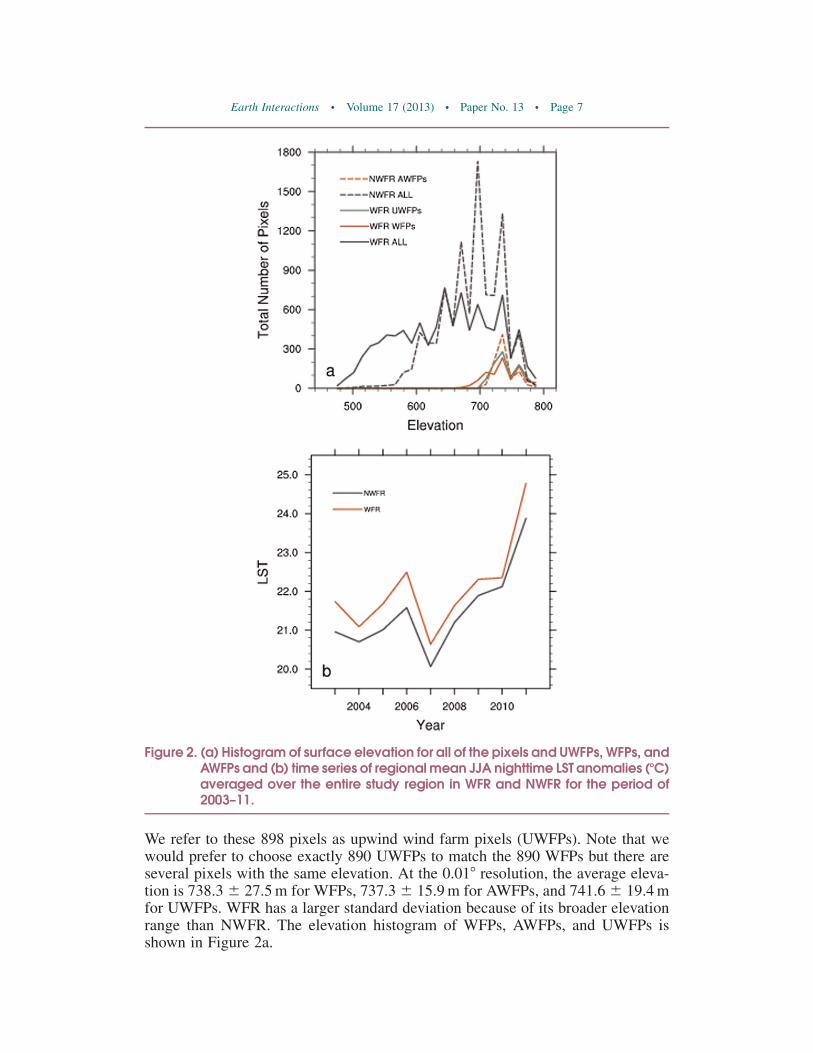
We refer to these 898 pixels as upwind wind farm pixels (UWFPs). Note that wewould prefer to choose exactly 890 UWFPs to match the 890 WFPs but there areseveral pixels with the same elevation. At the 0.018 resolution, the average eleva-tion is 738.36 27.5m for WFPs, 737.36 15.9m for AWFPs, and 741.66 19.4mfor UWFPs. WFR has a larger standard deviation because of its broader elevationrange than NWFR. The elevation histogram of WFPs, AWFPs, and UWFPs isshown in Figure 2a.

Figure 2. (a) Histogram of surface elevation for all of the pixels and UWFPs, WFPs, andAWFPs and (b) time series of regionalmean JJA nighttime LST anomalies (8C)averaged over the entire study region in WFR and NWFR for the period of2003–11.


To quantify the wind farm impact, Zhou et al. (Zhou et al. 2012) compared theLSTs of 890 WFPs with 1538 nearby nonwind farm pixels for WFR. For NWFR,we randomly choose 1538 pixels around the 890 AWFPs following the elevationhistogram of the 1538 pixels in WFR as their corresponding nearby nonwind farmpixels. At the 0.018 resolution, the average elevation for these 1538 pixels is661.2 6 55.6 m in WFR and 661.7 6 14.8 m in NWFR.

2.3. Methods

The LST variations consist of two components: the background regional- orlarge-scale variability signal (referred to as regional interannual variability) and thesubregional-scale variability. The former is much larger than the latter in magni-tude and is irrelevant to wind farms. Particularly, the two study regions are smalland close to each other, and thus their pixels should share a similar backgroundsignal. Figure 2b shows the regional mean JJA nighttime LST anomalies averagedover the entire domain inWFR and NWFR, respectively, for the period of 2003–11.The study regions exhibit strong year-to-year variations, with the coldest year in2007 and the warmest year in 2011 when the historic Texas drought occurred(Karl et al. 2012). Evidently, WFR and NWFR have gone through similar me-teorological conditions from 2003 to 2011 and have been getting warmer since2007. Because our analysis is interested in the variability on spatial scales smallerthan regional, we remove this background regional interannual variability signalfrom the MODIS LSTanomalies created in section 2.2 for each LST image. In otherwords, we subtract the same regional mean LSTanomaly (one value per image) fromthe MODIS LST anomaly for every pixel in each year to emphasize the pixel-levelLST spatial variability. Note that the resulting LST change represents a changerelative to the regional mean value and is denoted as DLST.

Three different methods are used to quantify the topographic effect on LSTsover our study regions. The first method (method I) applies a simple EOF analysisto the MODIS DLSTs. The EOF method has been extensively used to analyze thespatial and temporal variability of geophysical fields by decomposing the data intoa set of orthogonal basis functions (Bjornsson and Venegas 1997). Its goal is toexpress the signal in terms of a relatively small number of EOFs to describe asmuch of the original information as possible. The EOF modes show the spatialstructure of the major factors that can account for the temporal variations, whichrepresent spatial variability or ‘‘modes of variability.’’ The EOF time series tellsus how the amplitude of each EOF mode varies with time. The first few EOFs mayexplain the majority of the data variance and thus the inversion of the EOF trans-form using only the first few EOFs provides a noise-filtered dataset.

Note that, even though the EOF method breaks the data into modes of variability,these modes are primarily data modes and not necessarily ‘‘physical modes,’’ andwhether they are physical is a matter of subjective interpretation (Bjornsson andVenegas 1997). The first EOF mode would explain more than 94% of the totalDLST variance in WFR and NWFR if one simply performed the EOF analysisusing the MODIS LST anomalies. For this case, EOF1 would represent primarilythe climatology of DLSTand its time series would represent the regional mean LSTanomalies from 2003 to 2011 (as shown in Figure 2b). This explains why we removethe background regional interannual variability signal from the MODIS LST


anomalies as described above. One similar example for doing so is the removalof the seasonal cycle of meteorological data before performing EOF analysis, asthis signal dominates everything else (Bjornsson and Venegas 1997).

The second and third methods (methods II and III) are adopted from the spatialpattern and time series analyses over WFR in Zhou et al. (Zhou et al. 2012; Zhouet al. 2013) but are used here as a new analysis of topographic effects on LST toprimarily supplement and compare with the EOF results over both WFR andNWFR given the short record of the MODIS data. Method II simply calculates theDLST differences at pixel level between two periods, 2009–11 and 2003–05 (thelast 3 years versus the first 3 years of data), and examines their spatial couplingwith wind turbines. This method is reasonable as there are only 111 wind turbinesin 2003 but 2358 in 2011 over WFR. Note that the DLST differences between twoindividual years (2010 minus 2003) are also examined in Zhou et al. (Zhou et al.2012) but will not be used here, as the results are similar to the differences betweenthe two periods. Method III quantifies the areal mean DLST differences betweenWFPs (AWFPs) and their nearby nonwind farm pixels in WFR (NWFR) from 2003to 2011, as done in urban heat island studies (Zhou et al. 2012). Zhou et al.(Zhou et al. 2013) used three different approaches to quantify DLST but ob-tained consistent results. Here we simply use one of the approaches, the total trend(trend per year3 8 years of intervals) estimated from the least squares fitting, as thenumber of operational wind turbines has increased with time since 2003.

3. Results and discussionTo understand how LST changes with varied elevation, we examine the spatial

patterns of the surface elevation and the JJA nighttime LST climatology over WFRand NWFR. As expected, LST drops with elevation increase (Liu et al. 2009;Minder et al. 2010) and so the valleys and plains are generally warmer than theridges and the lowest temperatures are observed in the highest elevations (figuresomitted for brevity). The spatial correlation coefficient between elevation and LSTis20.6 for WFR and20.46 for NWFR, which are statistically significant given thelarge size of samples (p � 0.05; n 5 9600 pixels). The correlation is not close to1 as spatial variations in land surface properties other than surface elevation (e.g.,vegetation amount and type) also play a role in determining the climatology of LST.

The first three EOF modes explain more than 66.6% of the total DLST variancefor both regions: 29.1%, 22.4%, and 15.1% for WFR and 34.6%, 18.4%, and 13.8%for NWFR. For WFR, there is a strong spatial coupling in EOF1 between positiveDLSTs and WFPs (Figure 3a), and the corresponding time series (more discussionbelow) shows a persistent upward trend from 2003 to 2011. Positive DLSTs arealso seen in lower-elevation plain pixels in the northeastern part of WFR, but theyare much weaker in magnitude and spatially smaller than those in WFPs. ForNWFR, there is a weak spatial coupling between positive DLST and southernlower-elevation valleys in EOF1 (Figure 3b), and the time series does not show anevident trend from 2003 to 2009 (more discussion below). Negative DLSTs inEOF1 are generally located over northern ridge pixels of NWFR (Figure 3b) andthe western part of WFR (Figure 3a). Overall, EOF1 and its time series show awarming effect over higher-elevation WFPs in WFR but over lower-elevationvalleys in NWFR. EOF2 and EOF3 in WFR represent the spatial patterns of higher


DLSTs over lower elevations in the northeastern and southwestern parts of WFR,respectively, and their time series indicate a large interannual variation. There is nospatial coupling between the wind farms and DLSTs in EOF2 and EOF3 (figuresnot shown for brevity).

As mentioned above, the EOF modes are primarily data modes and not neces-sarily physical modes. To further attribute the EOF1 mode and its time series to thedevelopment of wind farms, we compared our results to those in Zhou et al. (Zhouet al. 2012). We use method II to calculate the DLST differences (2009–11 minus2003–05 averages) over WFR (Figure 3c) and NWFR (Figure 3d). The spatialcoupling between the warming effect and the wind turbines is evident in Figure 3cand this coupling is well captured by the EOF1 mode (Figure 3a), while there areno warming effects related to topography over NWFR in both Figures 3b and 3d.In general, EOF1 captures the major variations of DLST, as also indicated by thepercentage of variance explained. If the warming effect of WFPs in EOF1 overWFR was an artifact of topography, we would observe a similar warming effect ofAWFPs in EOF1 over NWFR. Furthermore, unlike EOF1 in WFR, EOFs 2 and 3 in

Figure 3. EOF1 of MODIS JJA nighttime DLST (8C) in (a) WFR and (b) NWFR for theperiod of 2003–11 and differences (2009–11 minus 2003–05 averages) ofMODIS JJA nighttime DLST (8C) in (c) WFR and (d) NWFR. Pixels with a plussymbol are WFPs in WFR and AWFPs in NWFR. Note that (c) and Figure 2adiffer slightly from Figure 2a of Zhou et al. (Zhou et al. 2012), as the latterwas calculated from the JJA LST means.


WFR and EOFs 1 and 2 in NWFR generally show negative DLSTs over higherelevations, consistent with the observational decrease of temperature with altitude(Liu et al. 2009; Minder et al. 2010).

Next we examine how the DLST vary as a function of surface elevation withinpixels. All of the 9600 pixels in the two study regions are divided equally into 10 binsin terms of surface elevation, with each bin having ;960 pixels. Note that somebins may have several pixels more or less than 960 because not every pixel has adifferent elevation. For each bin, we also consider two subgroups (WFPs andUWFPs) in WFR and one subgroup (AWFPs) in NWFR, if there are more than50 pixels present for each subgroup. The corresponding box-and-whisker chart ofEOF1 in WFR (Figure 4a) indicates that the minimum, 25th percentile, median,and 75th percentile DLSTs are always larger than those of pixels in similar ele-vation bins, suggesting a warming effect over WFPs relative to their similar sur-roundings. However, EOF1 of NWFR (Figure 4b) shows similar DLSTs in bothAWFPs and other pixels with similar elevation bins, suggesting no differencesbetween AWFPs and their similar surroundings. Also, it is interesting to note thatthe DLST generally decreases with elevation for all of the 10 bins in NWFR andalso for an elevation lesser than 700m in WFR. However, the DLST increases withan elevation greater than 700m with the presence of wind turbines in WFR. Thisincrease in WFR differs from NWFR and overlaps with the elevations where thewind farms are built, mainly because of the downwind effects of wind farms overpixels that are close to wind farms but have no wind turbines (Figures 3a,c). Thiscan be seen clearly from the DLST changes in UWFPs (Figure 4a). Figures 4c and4d illustrate the corresponding box-and-whisker chart of the DLST differencesbetween the averages of 2009–11 and those of 2003–05 as a function of elevationfor WFR and NWFR using method II. Again, WFPs are generally associated withhigher elevations and their DLSTs are often warmer than other pixels with similarelevations in WFR while AWFPs correspond to higher elevation but lower DLSTsin NWFR. The similarities between Figures 4a and 4c and between Figures 4b and4d indicate that our results from the two different methods are robust.

Zhou et al. (Zhou et al. 2012; Zhou et al. 2013) found that the warming effectover wind farms is the smallest in DJF and the strongest in JJA over WFR. Here weapply the EOF analysis (method I) to DJF and ANN and examine how DLSTchanges with elevation as done in Figure 4. For EOF1 in WFR, there is an increasein DLST in DJF with elevation, which differs from JJA, and the LSTs in WFPs areonly slightly higher than other pixels with similar elevations (Figure 5a). For EOF1in NWFR, the DJF DLST decreases with elevation and the DLSTs differ littlebetween AWFPs and other pixels with similar elevations (Figure 5a). The DLSTdifferences between the averages of 2009–11 and those of 2003–05 (Figure 5b) aresimilar to those in EOF1 (Figure 5a). As expected, the results of ANN show similarfeatures as those in JJA but with a smaller magnitude in terms of DLST changes.Again, our two different methods (methods I and II) provide consistent results inboth WFR and NWFR.

Results of Figures 4 and 5 show that the DLST means between three subgroupsof pixels (WFPs, UWFPs, and AWFP) differ from their surroundings pixels withsimilar elevations. Given the large variation of sample size among different groupsand different elevation bins, it is necessary to test (i) whether the DLST meansof WFPs differ statistically significantly from those of other pixels with similar


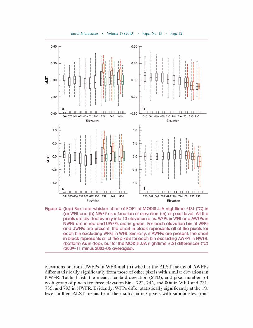
elevations or from UWFPs in WFR and (ii) whether the DLST means of AWFPsdiffer statistically significantly from those of other pixels with similar elevations inNWFR. Table 1 lists the mean, standard deviation (STD), and pixel numbers ofeach group of pixels for three elevation bins: 722, 742, and 806 in WFR and 731,735, and 793 in NWFR. Evidently, WFPs differ statistically significantly at the 1%level in their DLST means from their surrounding pixels with similar elevations

Figure 4. (top) Box-and-whisker chart of EOF1 of MODIS JJA nighttime DLST (8C) in(a) WFR and (b) NWFR as a function of elevation (m) at pixel level. All thepixels are divided evenly into 10 elevation bins. WFPs in WFR and AWFPs inNWFR are in red and UWFPs are in green. For each elevation bin, if WFPsand UWFPs are present, the chart in black represents all of the pixels foreach bin excluding WFPs in WFR. Similarly, if AWFPs are present, the chartin black represents all of the pixels for each bin excluding AWFPs in NWFR.(bottom) As in (top), but for the MODIS JJA nighttime DLST differences (8C)(2009–11 minus 2003–05 averages).


and from UWFPs for almost all of the 18 cases (3 elevation bins 3 3 seasons 32 methods). The only exception is the case for the highest-elevation bin (806m) inDJF, which is expected as the wind farm impact is the weakest in DJF (Zhou et al.2012). It is interesting to note that the DLST differences between WFPs and theirsurrounding pixels with similar elevations or between WFPs and UWFPs becomesmaller with the increase of elevation, which is also seen in Figures 4 and 5,suggesting that the impact of wind farms decreases with elevation. In NWFR, theDLST means of AWFPs are not different statistically from those of their sur-rounding pixels with similar elevations for all of the 18 cases, even at the 10%significance level.

Figure 5. (top) Box-and-whisker chart of MODIS DJF nighttime DLST (8C) in WFR andNWFR from (a) EOF1 and (b) the differences (2009–11 minus 2003–05 av-erages) using method II as a function of elevation (m) at pixel level. Theelevation bins and colors are defined as in Figure 4. (bottom) As in (top),but for MODIS ANN nighttime DLST.


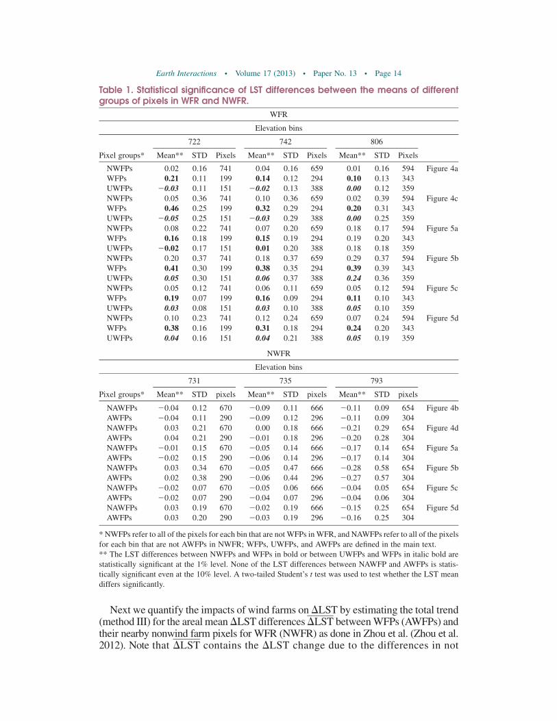
Next we quantify the impacts of wind farms on DLST by estimating the total trend(method III) for the areal meanDLST differencesDLST betweenWFPs (AWFPs) andtheir nearby nonwind farm pixels for WFR (NWFR) as done in Zhou et al. (Zhou et al.2012). Note that DLST contains the DLST change due to the differences in not

Table 1. Statistical significance of LST differences between the means of differentgroups of pixels in WFR and NWFR.

WFR

Elevation bins

722 742 806

Pixel groups* Mean** STD Pixels Mean** STD Pixels Mean** STD Pixels

NWFPs 0.02 0.16 741 0.04 0.16 659 0.01 0.16 594 Figure 4aWFPs 0.21 0.11 199 0.14 0.12 294 0.10 0.13 343UWFPs 20.03 0.11 151 20.02 0.13 388 0.00 0.12 359NWFPs 0.05 0.36 741 0.10 0.36 659 0.02 0.39 594 Figure 4cWFPs 0.46 0.25 199 0.32 0.29 294 0.20 0.31 343UWFPs 20.05 0.25 151 20.03 0.29 388 0.00 0.25 359NWFPs 0.08 0.22 741 0.07 0.20 659 0.18 0.17 594 Figure 5aWFPs 0.16 0.18 199 0.15 0.19 294 0.19 0.20 343UWFPs 20.02 0.17 151 0.01 0.20 388 0.18 0.18 359NWFPs 0.20 0.37 741 0.18 0.37 659 0.29 0.37 594 Figure 5bWFPs 0.41 0.30 199 0.38 0.35 294 0.39 0.39 343UWFPs 0.05 0.30 151 0.06 0.37 388 0.24 0.36 359NWFPs 0.05 0.12 741 0.06 0.11 659 0.05 0.12 594 Figure 5cWFPs 0.19 0.07 199 0.16 0.09 294 0.11 0.10 343UWFPs 0.03 0.08 151 0.03 0.10 388 0.05 0.10 359NWFPs 0.10 0.23 741 0.12 0.24 659 0.07 0.24 594 Figure 5dWFPs 0.38 0.16 199 0.31 0.18 294 0.24 0.20 343UWFPs 0.04 0.16 151 0.04 0.21 388 0.05 0.19 359

NWFR

Elevation bins

731 735 793

Pixel groups* Mean** STD pixels Mean** STD pixels Mean** STD pixels

NAWFPs 20.04 0.12 670 20.09 0.11 666 20.11 0.09 654 Figure 4bAWFPs 20.04 0.11 290 20.09 0.12 296 20.11 0.09 304NAWFPs 0.03 0.21 670 0.00 0.18 666 20.21 0.29 654 Figure 4dAWFPs 0.04 0.21 290 20.01 0.18 296 20.20 0.28 304NAWFPs 20.01 0.15 670 20.05 0.14 666 20.17 0.14 654 Figure 5aAWFPs 20.02 0.15 290 20.06 0.14 296 20.17 0.14 304NAWFPs 0.03 0.34 670 20.05 0.47 666 20.28 0.58 654 Figure 5bAWFPs 0.02 0.38 290 20.06 0.44 296 20.27 0.57 304NAWFPs 20.02 0.07 670 20.05 0.06 666 20.04 0.05 654 Figure 5cAWFPs 20.02 0.07 290 20.04 0.07 296 20.04 0.06 304NAWFPs 0.03 0.19 670 20.02 0.19 666 20.15 0.25 654 Figure 5dAWFPs 0.03 0.20 290 20.03 0.19 296 20.16 0.25 304

* NWFPs refer to all of the pixels for each bin that are not WFPs inWFR, and NAWFPs refer to all of the pixelsfor each bin that are not AWFPs in NWFR; WFPs, UWFPs, and AWFPs are defined in the main text.** The LST differences between NWFPs and WFPs in bold or between UWFPs and WFPs in italic bold arestatistically significant at the 1% level. None of the LST differences between NAWFP and AWFPs is statis-tically significant even at the 10% level. A two-tailed Student’s t test was used to test whether the LST meandiffers significantly.


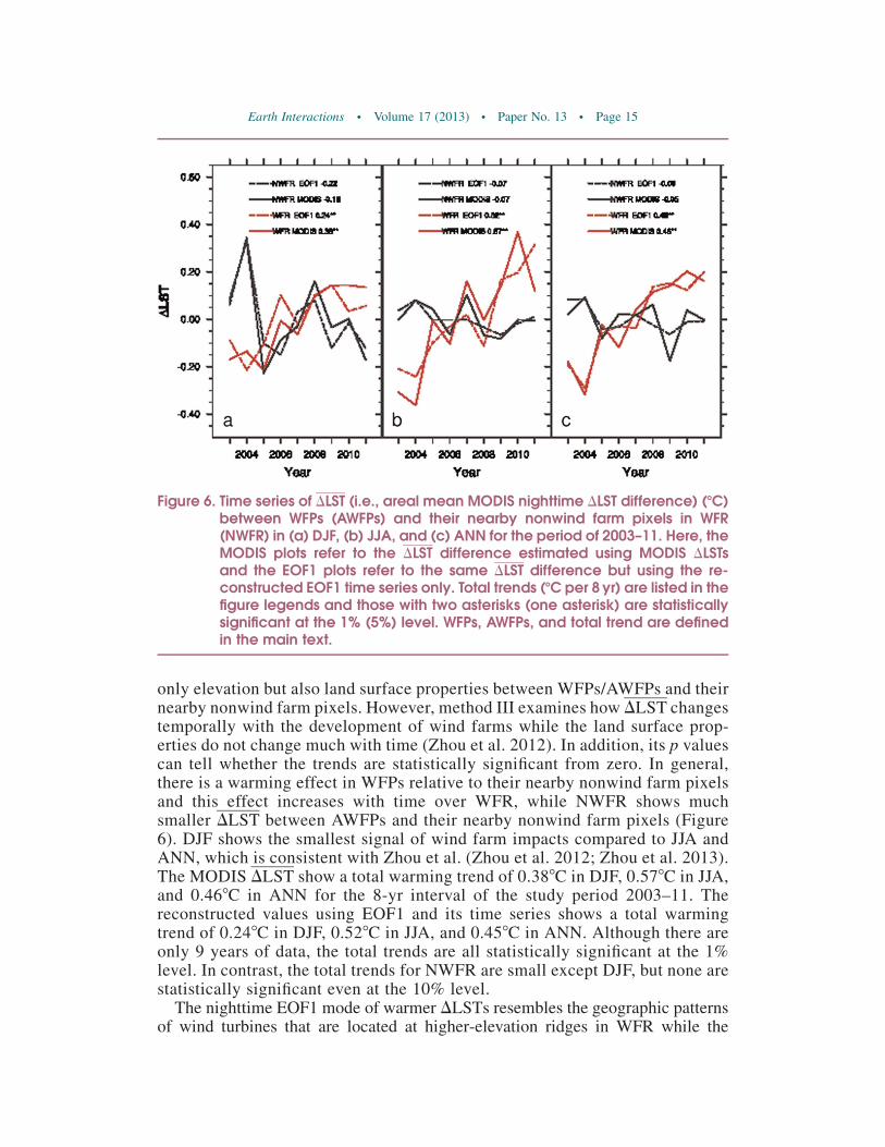
only elevation but also land surface properties between WFPs/AWFPs and theirnearby nonwind farm pixels. However, method III examines how DLST changestemporally with the development of wind farms while the land surface prop-erties do not change much with time (Zhou et al. 2012). In addition, its p valuescan tell whether the trends are statistically significant from zero. In general,there is a warming effect in WFPs relative to their nearby nonwind farm pixelsand this effect increases with time over WFR, while NWFR shows muchsmaller DLST between AWFPs and their nearby nonwind farm pixels (Figure6). DJF shows the smallest signal of wind farm impacts compared to JJA andANN, which is consistent with Zhou et al. (Zhou et al. 2012; Zhou et al. 2013).The MODIS DLST show a total warming trend of 0.388C in DJF, 0.578C in JJA,and 0.468C in ANN for the 8-yr interval of the study period 2003–11. Thereconstructed values using EOF1 and its time series shows a total warmingtrend of 0.248C in DJF, 0.528C in JJA, and 0.458C in ANN. Although there areonly 9 years of data, the total trends are all statistically significant at the 1%level. In contrast, the total trends for NWFR are small except DJF, but none arestatistically significant even at the 10% level.

The nighttime EOF1 mode of warmer DLSTs resembles the geographic patternsof wind turbines that are located at higher-elevation ridges in WFR while the

Figure 6. Time series of DLST (i.e., areal mean MODIS nighttime DLST difference) (8C)between WFPs (AWFPs) and their nearby nonwind farm pixels in WFR(NWFR) in (a) DJF, (b) JJA, and (c) ANN for the period of 2003–11. Here, theMODIS plots refer to the DLST difference estimated using MODIS DLSTsand the EOF1 plots refer to the same DLST difference but using the re-constructed EOF1 time series only. Total trends (8C per 8yr) are listed in thefigure legends and those with two asterisks (one asterisk) are statisticallysignificant at the 1% (5%) level. WFPs, AWFPs, and total trend are definedin the main text.


warmer DLSTs are observed over lower-elevation plains and valleys in NWFR.This contrast indicates a possible link between the warming effect over WFPs andthe development of wind farms. The gradual strengthening of the spatial couplingof EOF1 mode with wind turbines in WFR is expected, as wind turbines wereconstructed in stages, with more wind turbines built and likely operating with timefrom 2003 to 2011. This spatial coupling does not imply causation. However, Zhouet al. (Zhou et al. 2012; Zhou et al. 2013) have examined possible contributors tothe LST changes and found that the diurnal and seasonal variations in wind speedand the changes in near-surface ABL conditions due to wind farm operations arelikely the primary causes.

4. ConclusionsThis paper applies the empirical orthogonal function (EOF) analysis to de-

compose satellite-derived nighttime land surface temperature (LST) for the periodof 2003–11 into spatial patterns of different scales and thus to identify whether(i) there is a pattern of LST change associated with the development of wind farmsand (ii) the warming effect over wind farms reported previously is an artifact ofvaried surface topography. The spatial pattern and time series analysis approachesof Zhou et al. (Zhou et al. 2012; Zhou et al. 2013) are also used to supplement andcompare with the EOF results. Two equal-sized regions with similar topographyin west-central Texas are chosen to represent a wind farm region (WFR) and anonwind farm region (NWFR).

Our results indicate that the nighttime warming effect seen in the first mode(EOF1) in WFR very likely represents the wind farm impacts as its spatial patterncouples very well with the geographic distribution of wind turbines, which aregenerally built on high-elevation ridges. The time series associated with the EOF1mode in WFR also shows a persistent upward trend over wind farms from 2003 to2011, corresponding to the increase of operating wind turbines with time. Also, thewind farm pixels show distinctly warmer LST changes from their upwind high-elevation pixels and their downwind nonwind farm pixels at similar elevations. It isinteresting to note that the warming effect of wind farms decreases with elevation.In contrast, NWFR shows a decrease in LST with elevation, indicating that thepresence of wind farms inWFR has changed the LST–elevation relationship shownin NWFR. The elevation impacts on MODIS LST, if any, are much smaller andstatistically insignificant than the strong and persistent signal of wind farm im-pacts. While the MODIS data may be too short to draw any definite conclusions,these results are consistent with those in Zhou et al. (Zhou et al. 2012; Zhou et al.2013) and provide further observational evidence of the impacts of wind farms onLST. They also indicate that EOF analysis helps to decompose the MODIS LSTsinto different spatial patterns and thus can be used to detect and quantify theimpacts of wind farms at local scales.

Acknowledgments. We are grateful to two anonymous reviewers for their constructivecomments, which have helped to substantially improve the paper. This study was sup-ported by the startup funds provided by University at Albany, State University of New Yorkand by National Science Foundation (NSF AGS-1247137). H. Chen was supported by theNational Basic Research Program of China (Grant 2011CB952000). Y. Dai was supported


by the National Natural Science Foundation of China under Grant 40875062 and the 111Project of Ministry of Education and State Administration for Foreign Experts Affairs ofChina.

References

AWEA, 2012: The AWEA U.S. wind industry annual market report year ending 2011. AmericanWind Energy Association Rep., 94 pp.

Baidya Roy, S., and J. J. Traiteur, 2010: Impacts of wind farms on surface air temperatures. Proc.Natl. Acad. Sci. USA, 107, 17 899–17 904.

Bjornsson, H., and S. A. Venegas, 1997: A manual for EOF and SVD analyses of climatic data.McGill University CCGCR Rep. 97-1, 54 pp. [Available online at http://www.geog.mcgill.ca/gec3/wp-content/uploads/2009/03/Report-no.-1997-1.pdf.]

Fiedler, B. H., and M. S. Bukovsky, 2011: The effect of a giant wind farm on precipitation in aregional climate model. Environ. Res. Lett., 6, 045101, doi:10.1088/1748-9326/6/4/045101.

Fitch, A. C., J. K. Lundquist, and J. B. Olson, 2013: Mesoscale influences of wind farms throughouta diurnal cycle. Mon. Wea. Rev., 141, 2173–2198.

Imhoff, M. L., P. Zhang, R. E. Wolfe, and L. Bounoua, 2010: Remote sensing of the urban heatisland effect across biomes in the continental USA. Remote Sens. Environ., 114, 504–513.

Jin, M., and R. E. Dickinson, 2002: New observational evidence for global warming from satellite.Geophys. Res. Lett., 29, doi:10.1029/2001GL013833.

Karl, T. R., and Coauthors, 2012: U.S. temperature and drought: Recent anomalies and trends. Eos,Trans. Amer. Geophys. Union, 93, 473, doi:10.1029/2012EO470001.

Keith, D. W., J. F. DeCarolis, D. C. Denkenberger, D. H. Lenschow, S. L. Malyshev, S. Pacala, andP. J. Rasch, 2004: The influence of large-scale wind power on global climate. Proc. Natl.Acad. Sci. USA, 101, 16 115–16 120.

Kirk-Davidoff, D. B., and D. W. Keith, 2008: On the climate impact of surface roughness anom-alies. J. Atmos. Sci., 65, 2215–2234.

Lipton, A. E., and J. M. Ward, 1997: Satellite-view biases in retrieved surface temperatures inmountain areas. Remote Sens. Environ., 60, 92–100.

Liu, Y., Y. Noumi, and Y. Yamaguchi, 2009: Discrepancy between ASTER- and MODIS-derivedland surface temperatures: Terrain effects. Sensors, 9, 1054–1066, doi:10.3390/s90201054.

Minder, J. R., P. W. Mote, and J. D. Lundquist, 2010: Surface temperature lapse rates over complexterrain: Lessons from the Cascade Mountains. J. Geophys. Res., 115, D14122, doi:10.1029/2009JD013493.

NRC, 2007: Environmental Impacts of Wind-Energy Projects. National Academies Press, 377 pp.Pacala, S., and R. Socolow, 2004: Stabilization wedges: Solving the climate problem for the next

50 years with current technologies. Science, 305, 968–972, doi:10.1126/science.1100103.Pryor, S. C., and R. J. Barthelmie, 2011: Assessing climate change impacts on the near-term stability of

the wind energy resource over the United States. Proc. Natl. Acad. Sci. USA, 108, 8167–8171.Rajewski, D. A., and Coauthors, 2013 Crop Wind Energy Experiment (CWEX): Observations

of surface-layer, boundary layer, and mesoscale interactions with a wind farm. Bull. Amer.Meteor. Soc., 94, 655–672.

U.S. DOE, 2008: 20% wind by 2030: Increasing wind energy’s contribution to U.S. electricitysupply. U.S. Department of Energy Rep., 27 pp. [Available online at http://www1.eere.energy.gov/wind/pdfs/42864.pdf.]

——, 2012: Electric power monthly May 2012: With data for March 2012. U.S. Department ofEnergy Energy Information Administration Rep. DOE/EIA-0226 (2012/03), 180 pp. [Availableonline at http://www.eia.gov/electricity/monthly/current_year/may2012.pdf.]

Wan, Z., 2006: New refinements and validation of the MODIS land surface temperature/emissivityproducts. Remote Sens. Environ., 112, 59–74.


——, and Z.-L. Li, 1997: A physics-based algorithm for retrieving land-surface emissivity andtemperature from EOS/MODIS data. IEEE Trans. Geosci. Remote Sens., 35, 980–996.

Wang, C., and R. G. Prinn, 2010: Potential climatic impacts and reliability of very large-scale windfarms. Atmos. Chem. Phys., 10, 2053–2061.

Zhang, P., M. L. Imhoff, R. E. Wolfe, and L. Bounoua, 2010: Urban heat island effect across biomesin the continental USA. Proc. Int. Geoscience and Remote Sensing Symp., Honolulu, HI,IEEE, 1920–1923, doi:10.1109/IGARSS.2010.5653907.

Zhou, L., C. J. Tucker, R. K. Kaufmann, D. Slayback, N. V. Shabanov, and R. B. Myneni, 2001:Variations in northern vegetation activity inferred from satellite data of vegetation indexduring 1981 to 1999. J. Geophys. Res., 106 (D17), 20 069–20 083.

——, Y. Tian, S. Baidya Roy, C. Thorncroft, L. F. Bosart, and Y. Hu, 2012: Impacts of wind farmson land surface temperature. Nat. Climate Change, 2, 539–543.

——,——,——, Y. Dai, and H. Chen, 2013: Diurnal and seasonal variations of wind farm impactson land surface temperature over western Texas. Climate Dyn., 41, 307–326, doi:10.1007/s00382-012-1485-y.

Earth Interactions is published jointly by the American Meteorological Society, the American Geophysical

Union, and the Association of American Geographers. Permission to use figures, tables, and brief excerpts

from this journal in scientific and educational works is hereby granted provided that the source is

acknowledged. Any use of material in this journal that is determined to be ‘‘fair use’’ under Section 107 or that

satisfies the conditions specified in Section 108 of the U.S. Copyright Law (17 USC, as revised by P.IL. 94-

553) does not require the publishers’ permission. For permission for any other from of copying, contact one of

the copublishing societies.


effects of topography on assessing wind farm impacts using

Documents