effects of light and salinity stress on vallisneria

W&M ScholarWorks W&M ScholarWorks

Dissertations, Theses, and Masters Projects Theses, Dissertations, & Master Projects

2001

Effects of Light and Salinity Stress on Vallisneria americana (Wild Effects of Light and Salinity Stress on Vallisneria americana (Wild

Celery) Celery)

Gail T. French College of William and Mary - Virginia Institute of Marine Science

Follow this and additional works at: https://scholarworks.wm.edu/etd

Part of the Botany Commons

Recommended Citation Recommended Citation French, Gail T., "Effects of Light and Salinity Stress on Vallisneria americana (Wild Celery)" (2001). Dissertations, Theses, and Masters Projects. Paper 1539617774. https://dx.doi.org/doi:10.25773/v5-v10r-zt90

This Thesis is brought to you for free and open access by the Theses, Dissertations, & Master Projects at W&M ScholarWorks. It has been accepted for inclusion in Dissertations, Theses, and Masters Projects by an authorized administrator of W&M ScholarWorks. For more information, please contact [email protected].

https://scholarworks.wm.edu/

https://scholarworks.wm.edu/etd

https://scholarworks.wm.edu/etds

https://scholarworks.wm.edu/etd?utm_source=scholarworks.wm.edu%2Fetd%2F1539617774&utm_medium=PDF&utm_campaign=PDFCoverPages

http://network.bepress.com/hgg/discipline/104?utm_source=scholarworks.wm.edu%2Fetd%2F1539617774&utm_medium=PDF&utm_campaign=PDFCoverPages

https://dx.doi.org/doi:10.25773/v5-v10r-zt90

mailto:[email protected]

EFFECTS OF LIGHT AND SALINITY STRESS ON VALLISNERIA AMERICANA (WILD CELERY)

A Thesis

Presented to

The Faculty of the School of Marine Science

The College of William and Mary in Virginia

In Partial Fulfillment

Of the Requirements for the Degree of

Master of Science

by

Gail T. French 2001

APPROVAL SHEET

This thesis is submitted in partial fulfillment of

the requirements for the degree of

Master of Science

Gail T. French

Approved, August 2001

/Kenneth A. Moore, Ph.D. Committee Chairman/Advisor

DZ-p

Robert J. Orth, Ph.D.

AJames E. Perry, III, Ph.D

TABLE OF CONTENTS

Page

ACKNOWLEDGMENTS............................................................................................... v

LIST OF TA BLES.......................................................................................................... vi

LIST OF FIGURES........................................................................................................ vii

ABSTRACT................................................................................................................... viii

INTRODUCTION.............................................................................................................2

Ecology of Vallisneria americana ................................................................... 3

Pulse-Amplitude Modulated Fluorometry..................................................... 13

Objectives............................................................................................................ 18

Hypotheses..........................................................................................................19

METHODS.......................................................................................................................20

Experimental Systems................................................................................... 20

Measurements..................................................................................................24

Statistical Analyses.........................................................................................29

RESULTS.........................................................................................................................31

Environmental Conditions..............................................................................31

Morphology and Production...........................................................................38

Reproductive Structures..................................................................................68

Photosynthesis.................................................................................................. 68

DISCUSSION..................................................................................................................92

Morphology and Production...........................................................................92

Photosynthesis................................................................................................ 105

Reproduction...................................................................................................114

Applicability of Results to Field Conditions..............................................116

Determination of Light and Salinity Tolerance Limits.............................119

APPENDIX.................................................................................................................... 123

Salin ity .............................................................................................................. 123

Sediment Organic Carbon Content................................................................ 125

p H .......................................................................................................................127

Flowering Structures....................................................................................... 128

PAM Sample S ize ........................................................................................... 129

LITERATURE CITED.................................................................................................130

VITA................................................................................................................................140

iv

ACKNOWLEDGMENTS

This project would not have been possible without the unwavering guidance, patience, and good humor of my major professor, Dr. Ken Moore. I could not have imagined a better advisor. I also wish to thank my other Advisory Committee members, Dr. Bob Orth, Dr. Jim Perry, Dr. Linda Schaffner, and Dr. Peter van Veld, for their insightful recommendations. I am especially grateful to Dr. Orth for his boundless enthusiasm and support.

I am indebted to everyone who helped with mesocosm construction and maintenance, data collection, and laboratory analyses, including: Whitney Bishop, Dave Combs, Sara Everett, Curtis Copeland, Amy MacDonald, Alan Moore, Betty Berry Neikirk, Kevin Segerblom, Eric Slominski, Rachel Smith, Amy Tillman, Schuyler Van Montfrans, and Denise Wilson. Special thanks are extended to Jamie Fishman for advice on various aspects of this project, David Wilcox for computer help, Peter Ralph for his valuable instruction and insight on chlorophyll a fluorescence and Jennifer Rhode, Rom Lipcius, and Scott Marion for statistics help. Perhaps equally as important, I am grateful to all the wonderful people in Dr. Moore and Dr. Orth’s labs for keeping me relatively sane throughout my tenure at VIMS.

Financial support for portions of this study was received from Norfolk Southern and the City of Hopewell.

V

LIST OF TABLES

Table Page

1. Light and Salinity Studies on V. americana.................................................... 14

2. L igh t..................................................................................................................... 23

3. Salinity.................................................................................................................33

4. Grain Size.............................................................................................................33

5. p H ..........................................................................................................................39

6. Repeated Measures ANOVA R esults............................................................. 41

7. 2-Way ANOVA Results: Morphology, Production, and Reproduction.... 44

8. Chlorophyll ANOVA R esults...........................................................................71

9. Quantum Yield ANOVA Results..................................................................... 77

10. ETR ANOVA Results........................................................................................87

11. Summary of Light and Salinity Effects........................................................... 91

vi

LIST OF FIGURES

Figure Page

1. Distribution............................................................................................................ 62. Mesocosm Diagram............................................................................................213. Irradiance............................................................................................................. 324. Water Column D IN ............................................................................................355. Water Column PO4"3...........................................................................................366. Tem perature........................................................................................................377. Leaf Length.........................................................................................................408. Maximum Length...............................................................................................439. Elongation R ate.................................................................................................. 4710. Leaf W idth........................................................................................................... 4911. Width at Maximum Length...............................................................................5012. Leaf production per Rosette..............................................................................5213. Vegetative Reproduction................................................................................... 5314. Maximum Rosette Density................................................................................5515. Aboveground Biomass...................................................................................... 5816. Aboveground Biomass per Rosette..................................................................5917. Belowground Biom ass...................................................................................... 6118. Belowground Biomass per Rosette..................................................................6219. Leaf Area Index.................................................................................................. 6420. Aboveground Biomass per Leaf A rea............................................................. 6521. Leaf Area per Rosette.........................................................................................6622. Leaf Length * W idth..........................................................................................6723. Tubers...................................................................................................................6924. Chlorophyll, July 6 .............................................................................................7225. Chlorophyll, August 2 ....................................................................................... 7326. Chlorophyll, September 2 9 ...............................................................................7527. Effective Quantum Y ield ..................................................................................7828. Maximum Quantum Y ield ................................................................................8029. Initial Fluorescence............................................................................................8230. Maximum Fluorescence.................................................................................... 8331. RLC, August 20.................................................................................................. 8532. RLC, September 12............................................................................................8633. ETRmax..................................................................................................................8834. Ik, August 20........................................................................................................8935. Interactions........................................................................................................ 103

vii

ABSTRACT

The effects of light and salinity on Vallisneria americana (wild celery) were studied in outdoor mesocosms for an entire growing season. Morphology, production, photosynthesis, and reproductive output were monitored from tuber sprouting to plant senescence under four salinity (0, 5, 10, and 15 psu) and three light (2, 8, and 28% of surface irradiance) regimes. Chlorophyll a fluorescence was used to examine photochemical efficiency and electron transport rate. High salinity and low light each negatively influenced plant growth and reproduction. Production (biomass, rosette production, and leaf area index) was affected more by salinity than by light, apparently because of morphological plasticity (increased leaf length and width), increased photosynthetic efficiency, and increased chlorophyll concentrations under low light. Conversely, high salinity resulted in decreased photosynthetic efficiency, morphological changes that compounded salinity stress (reduced leaf elongation), and no change in chlorophyll concentrations. Light and salinity stresses were additive for morphological and photosynthetic characteristics. Although fluorescence parameters were correlated with physical symptoms of light and salinity stress, they did not predict reduced growth or death. Maximum electron transport rate (ETRmax) was highest in the 28% light treatment, indicating increased photosynthetic capacity. ETRmax was not, however, related to salinity, suggesting that the detrimental effects of salinity on production were through decreased photochemical efficiency and not decreased photosynthetic capacity. Light and salinity effects were interactive for measures of production, with negative salinity effects most apparent under high light conditions, and light effects found primarily at low salinity levels. The difference between responses of production and morphological measures may be due to the effects of light and salinity stress on a morphological characteristic compounding effects on another morphological characteristic or on photosynthesis, thus disproportionately decreasing production. For most production and morphology parameters, high light ameliorated salinity stress to a limited degree, but only between the 0 and 5 psu regimes. Growth was generally minimal in all of the 10 and 15 psu treatments, regardless of light level. Growth was also reduced at 2 and 8% light. The 28% light treatment was approximately at saturating levels, but did not cause photoinhibition. In addition, flowering and tuber production were impaired at 10 and 15 psu and at 2 and 8% light. Thus, upper salinity tolerance was between 5 and 10 psu, and light requirements may have been between 8 and 28% light. However, light requirements at 5 psu may be approximately 50% higher than at 0 psu. Results suggest that improving water clarity in the Chesapeake Bay may increase distribution, but only into regions less than 10 psu. The period May through July appears to be more important for resource procurement and colonization; thus, transplanting may be more successful at this time. Because of the interaction between salinity and light requirements for growth, effective management of SAV requires that growth requirements incorporate the effects of combined stressors.

EFFECTS OF LIGHT AND SALINITY STRESS ON VALLISNERIA AMERICANA (WILD CELERY)

2

INTRODUCTION

Over the past thirty years, distribution and abundance of rooted angiosperms, or

submersed aquatic vegetation (SAV), in the Chesapeake Bay has fluctuated at levels well

below historical levels (Bayley et al. 1978, Orth and Moore 1983, Orth and Moore 1984,

Twilley and Barko 1990). Declines have been related in large part to water quality

conditions that directly or indirectly limit light availability to the submersed plants for

growth (Kemp et al. 1983, Moore et al. 1996, Moore et al. 1997, Carter et al. 2000). Due

to the ecological and societal value of these submerged plant communities, extensive

research has been conducted to determine the causes of the decline and to define

optimum habitat characteristics for growth and reproduction. This information has been

used to set management goals and to evaluate sites for SAV restoration (Batiuk et al.

1992).

One poorly understood area of SAV ecology is the interaction between light

availability and salinity stress on plant response. In estuarine systems such as the

Chesapeake Bay turbidity levels are generally found to be inversely related to salinity,

with higher turbidities occurring in lower salinity regimes (Champ et al. 1980, Stevenson

et al. 1993, Moore et al. 1997). However, distribution of freshwater species generally

decreases at higher salinities (Moore et al. 2000a). Therefore, greater understanding of

the interactive effects of salinity and light availability on SAV growth can provide

important insights into the habitat requirements of SAV which are necessary for

improving conditions for restoration. With increasing development along shorelines

3

throughout the world, including the Chesapeake Bay, turbidity is rising (Dennison et al.

1993). Largely unknown is the effect of this increased turbidity alone. Also unknown is

whether there is an interactive effect between light and salinity. For instance, will

increased turbidity decrease salinity tolerance? Will lower salinity ameliorate light stress?

Answers to these questions will help us better manage the factors affecting SAV and

determine suitable areas for transplanting. Several short-term studies have indicated that

light stress may compound salinity stress (Kraemer et al. 1999, Ralph 1999c), but little is

known about the long-term (entire growing season) effects of these two stresses, either

individually or together. Also unclear is whether these stresses are interactive or additive.

In this study I evaluated the effects of different light and salinity regimes on the

SAV species Vallisneria americana throughout the growing season. I examined plant

response to environmental conditions using various measures of health, including plant

growth, morphology and biomass, photosystem characteristics, and reproductive output.

Ecology of Vallisneria americana

Taxonomy and morphology

Vallisneria americana (Michx.), also known as wild celery, tape grass, or eel-

grass, is a dioecious, freshwater, perennial aquatic plant (Lowden 1982) of the

Hydrocharitaceae family. It has linear submerged or floating leaves that can reach lengths

of 2 m or more. Its stem is vertical with a short axis and produces stolons and fibrous

roots (Lowden 1982). V. americana produces two basic forms: narrow- and broad-leaved.

The narrow-leaved variety bears leaves less than 10 mm wide with 3 to 5 distinct

longitudinal veins and smooth to finely toothed margins. It is found in lakes, lagoons, and

4

freshwater inland waterways. Leaves of the broad-leaved variety are 10 to 25 mm wide

with 5 to 9 veins and prominently toothed margins. It is found in coastal freshwater inlets

or spring-fed waterways subject to nearly constant temperature (Lowden 1982). The

narrow-leaved variety is the subject of this study.

Distribution

V. americana grows primarily in eastern North America, west from Nova Scotia

to South Dakota and south to the Gulf of Mexico (Korschgen and Green 1988). In the

Chesapeake Bay, V. americana has historically been one of the dominant freshwater and

low salinity species, inhabiting the upper Potomac, the upper James, and the upper

Chesapeake Bay, including the Susquehanna Flats and the Elk, Sassafras, Northeast and

Susquehanna rivers (Bayley et al. 1978, Haramis and Carter 1983, Twilley and Barko

1990, Moore et al. 2000a). It co-occurs most commonly with Myriophyllum spicatum and

Hydrilla verticillata (Moore et al. 2000a).

Unfortunately, historical distribution studies do not generally distinguish between

V. americana and other species in the typical freshwater SAV community (Moore et al.

2000a), so tracing historical changes in V. americana abundance requires the assumption

that V. americana has followed the patterns of other freshwater species.

Throughout the last half century, freshwater SAV abundance in the Chesapeake

Bay has fluctuated greatly. For example, in the tidal Potomac River the areal distribution

of submersed macrophyte species in 1981 was less than 25% of that in 1960 (Haramis

and Carter 1983). This decline has been related to increased nutrient and sediment inputs.

This same area experienced SAV resurgence in 1983 and 1984 (Twilley and Barko

5

1990). This comeback has been attributed to increased water clarity, a result of

improvements in sewage treatment and unusual weather conditions (Dennison et al.

1993), as well as the introduction and rapid expansion of the exotic species Hydrilla

verticillata (Carter and Rybicki 1986, Orth et al. 1994). The tidal freshwater portions of

the James River are thought to have supported SAV growth until the m id-1940’s.

Currently, SAV is found only in some tributary creeks near the Chickahominy River

(Orth et al. 1999, Moore et al. 2000b). This decline may be due to any number of factors,

including reduced water clarity due to suspended solids and phytoplankton, high epiphyte

loads, poor sediment characteristics (i.e., high organic content), or physical limitation due

to biological or physical disturbance (Moore et al. 2000b). Although detailed records of

SAV distribution in the upper Chesapeake Bay do not exist for the early part of the

twentieth century and previously, it is likely that distribution is substantially less today

(Orth and Moore 1984). Currently, only 20% of the upper Chesapeake Bay that could

potentially support SAV is vegetated, and most vegetated areas are sparsely covered

(Dennison et al. 1993). V. americana is primarily found in the Susquehanna and Potomac

Rivers only (Fig. 1, from Moore et al. 2000a).

Freshwater SAV distribution has exhibited recent periods of increase. For

example, from 1985 to 1993 Chesapeake Bay freshwater SAV increased from 3,200 to

6,650 metric tons, or 3200 to 4800 ha (Moore et al. 2000a, Orth et al. 1999), suggesting

that water quality may be improving in certain areas.

6

Figure 1. Distribution of V. americana throughout tidal regions of the Chesapeake Bay. Dots indicate all observations of the species made between 1985 and 1999 (Moore et al. 2000a, and updated by VIMS SAV mapping program).

Susquehanna River

V. Americana Observations

Delaware Bay

Atlantic Ocean

10 0 10 20 30 40 50 Km

7

Reproduction

V. Americana primarily reproduces asexually, although it is capable of sexual

reproduction, as well. Shoots emerge in late spring, when temperatures reach 10-14°C,

from tubers (also called winter buds or turions) (Korschgen and Green 1988). Tubers are

generally buried 5-27 cm deep in the Potomac River (Carter and Rybicki 1985). Near the

end of the growing season in late summer, the production of rosettes, or leaf clusters,

stops and some rosettes develop one or more tubers on stolons that grow down into the

sediment (Titus and Stephens 1983). After tuber formation, the remaining stem tissue

degenerates and breaks free of the substrate, floating until it decomposes.

Sexual reproduction occurs more rarely than asexual reproduction, although it

may be critical for long distance dispersal and maintenance of genetic diversity. During

the 1978 growing season in Chenango Lake, New York, for instance, only 24% of

sampled rosettes flowered (Titus and Stephens 1983). In the Pamlico River estuary, North

Carolina, no germination from seeds was observed (Korschgen and Green 1988). Flowers

are generally produced in summer (Carter and Rybicki 1985, Korschgen and Green

1988). In late summer or early fall, some of the fruit capsules rupture and release a

gelatinous matrix containing seeds (Kaul 1978). Other fruits do not rupture until the

plants break free of the substrate and float away (Korschgen and Green 1988).

Habitat value

V. americana has many important ecological functions. Like other SAV species,

its roots, rhizomes, and stolons provide structural support and habitat for benthic algae

and invertebrates, and stabilize nearshore sediments, thus reducing erosion (Sculthorpe

1967). Its foliage provides shelter to many types of organisms and, during daylight hours,

a locally enriched oxygen supply (Sculthorpe 1967). It removes inorganic nutrients from

the water column, thereby suppressing algal growth (Stevenson et al. 1979). Beds also

provide habitat for a number of fish species, including bluegills (.Lepomis macrochirus),

pumpkinseeds (Lepomis gibbosus), and yellow perch (Perea flavescens). As a food

source, V. americana is a particularly desirable species for many types of organisms,

including common carp (Cyprinus carpio), muskrats (Ondatra zibethicus), and red-

bellied turtles (.Pseudemys rubriventris), as well as many species of invertebrates (Carter

and Rybicki 1985, Korschgen and Green 1988). Waterfowl, particularly the canvasback

duck (.Aythya valisineria) prefer this species to many other SAV species, and use V.

americana beds as feeding areas during migration. Waterfowl consume both shoot

material and tubers (Korschgen and Green (1988).

Salinity tolerance

V. americana is a freshwater species that generally exhibits moderate salinity

tolerance. Experimental studies by Bourn (1932, 1934, op. cit. Twilley and Barko 1990)

found that growth of V. americana peaked at 2.8 practical salinity units (psu), and no

growth occurred above salinities of 8.4 psu. Laboratory experiments by Haller et al.

(1974) showed that growth occurred between 0.17 and 3.33 psu, and no growth occurred

at 6.66 psu. In the field, the species has been observed in slightly oligohaline regions of

estuaries and saline lakes. Along the north shore of the Pamlico River estuary, for

instance, V. americana was observed in 78.1% of quadrats with a mean salinity of 5.3 psu

(range from 0 psu to 12.8 psu). In regions of a slightly higher salinity (mean of 7.6 psu,

9

range from 2.2 psu to 13.9 psu), however, no V. americana was found (Davis and

Brinson 1976, op. cit. Twilley and Barko 1990).

Several more recent studies, however, have indicated a higher salinity tolerance

for the species. In a mesocosm study by Twilley and Barko (1990), V. americana under

8% and 50% of surface irradiance not only grew at 12 psu, but also grew at the same rate

as plants at lower salinities. The higher salinity tolerance observed in this study was

attributed to experimental methodology, whereby plants were exposed to gradual changes

in salinity (1 psu per day up to 6 psu, and then 2 psu per day up to the final salinity of 12

psu). This gradual increase possibly allowed some osmoregulatory mechanism to operate

(Twilley and Barko 1990). The highest recorded salinity tolerance, however, exceeded 15

psu, observed by Kraemer et al. (1999). In this study adult plants were transplanted to

sites in the Caloosahatchee Estuary, FL. At one site (diffuse attenuation coefficient <2

m '1) plants survived up to 12 weeks where salinity ranged from 12 to 20 psu and survived

4-6 weeks when salinities exceeded 15 psu. Additionally, in an unpublished mesocosm

experiment Doering observed survival, but no net growth, for 6 weeks at 15 psu

(Kraemer et al. 1999).

Light Requirements

The light environment that a plant experiences is a function of many factors,

including plant morphology, shoot density, depth, epiphyte accumulation, and light

attenuation through the water column. Attenuation of photosynthetically active radiation

(PAR) may be affected by the water itself, which absorbs suspended sediments and

dissolved substances, which most strongly absorb blue wavelengths (Kirk 1994).

10

Attenuation can also be increased by algae, which can form mats or blooms that absorb

the red and blue wavelengths used for photosynthesis (Korschgen et al. 1997).

V. americana is a relatively shade-tolerant species. In a photosynthesis study

using plants in test tubes, Meyer et al. (1943) found that V. americana could survive at

lower light intensities than any of the four other species tested (Najas flexilis,

Potamogeton Richardsonii, Eloclea canadensis, and Heteranthera dubia). In fact, the

apparent photosynthesis of V. americana was still 25% of that at the surface when plants

were receiving only a maximum of 0.5% surface light. In the field, however, its

maximum depth of distribution ranges from less than 2 to 9% of surface irradiance

(Batiuk et al. 1992, Carter et al. 2000), and it is most commonly found within the 10%

photic zone (Carter and Rybicki 1985).

This species’ shade tolerance is unexplained by its morphological plasticity. Other

SAV species, such as Myriophyllum spicatum L. (Titus and Adams 1979), form surface

canopies to intercept light under turbid conditions. V. americana, in contrast, has a

limited potential for elongation and canopy formation (Barko et al. 1991). It is thus

hindered in its ability to concentrate photoreceptive biomass near the water surface in low

light conditions. It compensates for this morphological disadvantage, however, by a high

physiological adaptability to low light. Its low half-saturation constant (60-197 jamol m’2

1 ^ 1 s’ , compared to 164-365 pmol m'~ s’ of Myriophyllum spicatum L.) indicates that it is

efficient at fixing CCF at low light intensities (Titus and Adams 1979). It also acclimates

very rapidly to increasing light (Titus and Adams 1979).

While V. americana is not as morphologically plastic as many other SAV species

(Barko et al. 1991), it can undergo moderate change. For instance, it is capable of a

11

certain degree of stem elongation in reduced light conditions (8% compared to 50% of

light; Barko et al. 1982, Barko et al. 1991). Under low light, leaf surface area and

length:breadth ratio can also increase (Barko et al. 1982), even while shoot density and

biomass decrease (Barko et al. 1982, Barko et al. 1991, but see Twilley and Barko 1990).

The production of reproductive structures by V. americana has been found to be

affected by light intensity. Number, total biomass, and individual mass of tubers are

inversely related to light intensity (Korschgen et al. 1997). Shoots emerging from tubers

under laboratory conditions, however, have the capability to grow to a mean length of

44.0 cm in total darkness (Korschgen, unpublished data). Kimber et al. (1995) found that

while seed germination was insensitive to light level, seedling survival was higher and

growth was greater in the study’s higher two light levels (9 and 25% of light, versus 2

and 5%). Tuber production was restricted to these two light levels.

Effects of combined stressors

Several studies have demonstrated the interactive effects of light and other

environmental condition, such as temperature, CCU, or nutrients, on V. americana. Barko

et al. (1991) studied the interactive effects of light, sediment fertility, and inorganic

carbon availability. They found that only under high light (50% of light, versus 8%) did

the other two factors affect plant biomass. Other studies have shown that experimental

manipulation affects growth more when V. americana has adequate light. Barko et al.

(1982), for instance, manipulated light and temperature and found that plants were more

responsive to differences in temperature at optimal light levels (600 and 1500 jimol nT“

s-1, versus 100 Limol irf2 s-1), and vice versa.

12

The demonstrated interactive effects of light and other environmental conditions

have led only a few experimenters to investigate the existence of interactive effects of

light and salinity. Twilley and Barko (1990) addressed this question in a mesocosm study

using light levels of 8 and 50% light and salinities of 0, 2, 4, 6, and 12. After five weeks,

they measured indices of survival, including stem density and length, chlorophyll from

the apical 10 cm, epiphyte mass, N and P concentrations, and reproductive structures.

They found no difference in total biomass (above- or belowground) or stem density

among the five salinity treatments in either light treatment. Epiphytic mass increased with

increasing salinity. Stem length increased with increasing salinity, except at the highest

salinity, at which it decreased. Stem length also increased with decreasing light. There

was no difference in number of underground buds between treatments, and there were

very few flowers in any treatment. N and P concentrations increased with increasing

salinity (except at 12 psu, when P concentration was at its lowest), with no difference

between the light levels.

The field transplant study of Kraemer et al. (1999) also examined combined light

and salinity effects. Transplants at sites with greater water clarity (approximately 27 to

38% light) were more tolerant of salinity. They suggest that light may moderate

hypersaline stress by providing additional energy to maintain an appropriate osmotic

potential.

Although salinity-irradiance interactions are beginning to be understood,

significant gaps in our knowledge remain. For example, the long-term effects (at least

one growing season) of shading and of a range of salinities on growth are unknown. The

field study of Kraemer et al. (1999) was conducted for two 12-week periods only, and

13

salinity and light levels varied naturally throughout the seasons. It is thus impossible to

distinguish short-term versus long-term effects of the stressors. The mesocosm study of

Twilley and Barko (1990) was likely too short-term to produce many significant

differences between regimes. In addition, the lowest light level (8%) was higher than

many V. americana plants in natural conditions experience; thus, light was not likely

limiting.

Relevant studies on the effects of light and salinity on V. americana are

summarized in Table 1.

Photosvstem Processes

Pulse-amplitude Modulated Fluorometry

Although monitoring morphological characteristics of SAV may be instructive of

a population’s health, careful, regular measurements are often cumbersome. In addition,

examining purely physical traits may reveal SAV stress only once the population has

begun its decline. The sooner managers are able to detect stress, the better chance they

have at maintaining populations or identifying environmental stressors. A technique that

reveals stress immediately would, therefore, be of great value in SAV research and

management. One technique that is gaining popularity for its ease of use and potential

predictive capabilities is chlorophyll a fluorescence. This technique, which can evaluate

photosynthesis in situ, has only been applied to SAV in recent years, but has quickly

added to our understanding of SAV response to stressors. However, there remains much

to learn about its applications.

Table 1. Summary of studies on light and salinity effects on V. americana.

14

Location Methods Factors Results ReferenceLake Erie, OH

Leaf blades in test tubes submerged at different depths

Light High rate of photosynthesis at very low light, compared to other freshwater SAV spp.

Meyer 1943

Florida Adultstransplanted to microcosms

Salinity 0, 3 psu: growth; 7, 10 psu: survival but no growth; 13, 17 psu: death

Haller et al. 1974

Pamlico River, NC

Survey of natural plants

Salinity Survival at 5 psu, not 8 psu Davis andBrinson1976

University Bay, W l

Harvested adult plants

Light Low half-saturation constant, compared to Myriophyllum

Titus and Adams 1979

Mississippi Adultstransplanted into tanks

Light,Temp.

Growth increased from 100 to 600 pmol m'2 s '1) but did not increase at 1500. Ligth and temp, effects interacted.

Barko et al. 1982

Potomac R. Survey of natural plants

Light Plants found only to <10% light Carter and Rybicki 1985

Maryland Adultstransplanted into microcosms

Salinity,Nutrients

Growth substantially reduced at 6 psu, compared to 0 psu

Staver 1986

Maryland Adultstransplanted into microcosms

Light and Salinity

Few differences in growth at different light (8, 50%) or salinity (0, 2, 4, 6, 12 psu) levels

Twilley and Barko 1990

Mississippi Adultstransplanted into microcosms

Light,C 0 2,Nutrients

Growth greater at 550 than 125 pmol m‘ s '1

Barko et al. 1991

Upper Mississippi R „ W l

Seedstransplanted to outdoor pool at different depths

Light Seed germination insensitive to light level; seedling survival higher and growth greater at 9 and 25% light, versus 2 and 5% light

Kimber et al. 1995

Upper Mississippi R „ Wl

Tubers planted in outdoor ponds at different light levels

Light Tuber production inversely related to light

Korschgen et al. 1997

Caloosahatch ee Estuary, SW FL

Adults transplanted along estuarine gradient

Light and Salinity

Salinity tolerance - 1 5 psu at higher light levels

Kraemer et al. 1999

Potomac R. Transplantedsprigs

Light Artificial light increased growth Carter et al. 2000

15

Chlorophyll a fluorescence reveals information about photosystem II (PSD)

photochemical processes, such as the light adaptation, photosynthetic capacity, and

efficiency of PSII (Ralph et al. 1998). Chlorophyll a fluorescence has been used to study

terrestrial plants for decades but has only been applied to SAV since 1997, with the

development of Diving-PAM (pulse-amplitude modulated), a submersible fluorometer

(Walz, Germany). This device provides information in situ about the effective quantum

yield (AF/Fm’), maximal quantum yield (Fv/Fm, ( p s ii) , and electron-transport rate (ETR)

of photosystem operation (Genty et al. 1989).

Effective quantum yield, also known as the Genty parameter, is a measure of

photochemical energy conversion at PS II reaction centers under ambient light (Genty et

al. 1989). It is measured with light-adapted leaves and is dependent on ambient

irradiance. Effective quantum yield is determined as follows: initial fluorescence (F) is

measured; a saturation pulse is applied; and fluorescence (Fm’) is immediately measured

again. Yield is the ratio of (Fm’- F) to Fm’.

Quantum yield of PSII is maximized after dark adaptation, when all PSII reaction

centers are open (all primary acceptors are oxidized) and heat dissipation is minimal

(Genty et al. 1989, Maxwell and Johnson 2000). Maximal quantum yield, then, is

determined in the same manner as effective quantum yield, only dark-adapted leaves are

used. Maximal quantum yield indicates maximum photochemical efficiency and is

affected by photoinhibition and processes related to other stresses, such as heat and

salinity (the quantum yield will be lower when a plant is stressed) (Ralph 1998a, Ralph

1998b, Ralph 1999c). The notation for maximal quantum yield is (Fm-Fo)/Fm, or Fv/Fm,

16

where Fm is the maximum fluorescence, Fo is the minimum fluorescence, and Fv is the

variable fluorescence (Genty et al. 1989, Maxwell and Johnson 2000).

The PAM fluorometer may also be used to conduct rapid light curves (RLC). For

this technique light is applied to a leaf at nine increasing light intensities over the course

of several minutes. At each level ETR is calculated. ETR is a measure of electron

transport through the photochemical reactions, resulting in carbon fixation. It is derived

from a relationship between irradiance, leaf absorbance and the quantum yield (Ralph et

al. 1998). ETR then may be plotted against irradiance to create a RLC. A RLC enables

determination of the maximum ETR (ETRinax), the minimum saturating irradiance (R),

and the irradiance at which photoinhibition begins (Walz 1998). RLCs allow for an

examination of the photoadaptation of a plant (Ralph, pers. comm.). Chlorophyll a

fluorescence, then, can be used to detect not only stress but also adaptation.

One advantage of chlorophyll a fluorescence is that it provides a convenient

means to study photosynthesis in situ with minimal disturbance. Prior to the development

of Diving-PAM, SAV photosynthesis was measured by enclosing plants in chambers and

measuring gas exchange, or bringing samples back to the lab. PAM fluorometry not only

provides a quick, in situ measurement of photosynthesis but also allows for a study of

multiple aspects of photosynthesis, such as heat dissipation and electron transport. The

utility of PAM fluorometry as a surrogate for gas exchange studies has been supported by

research finding a direct relationship between CL evolution and ETR (Ralph and Burchett

1995, Beer and Bjork 2000).

17

Use of PAM fluorometry in the study of stressors on SAV

Since the development of Diving-PAM, numerous studies have examined the

effects of environmental stress on SAV using PAM fluorometry. Most of these studies

have used the effective quantum yield and maximal quantum yield as an indication of

stress response (Ralph and Burchett 1998a, Ralph and Burchett 1998b, Ralph 1998a,

Ralph 1998b, Longstaff et al. 1999, Ralph 1999a, Ralph 1999b, Ralph 1999c, Prange and

Dennison 2000). Yield declines with stress. The most common type of stress studied in

this context is high light. Other stressors include temperature (Ralph 1998b, Ralph

1999c), salinity (Ralph 1998a, Ralph 1999c), heavy metals (Ralph and Burchett 1998b,

Prange and Dennison 2000), herbicides (Ralph 1999a), and petrochemicals (Ralph and

Burchett 1998a).

PAM fluorometry studies on SAV have most often examined the effect of short

term light stress on quantum yield. High light can cause photoinhibition, resulting in

decreased photochemical efficiency (Ralph and Burchett 1995, Ralph 1999c). The effect

of long-term differences in light regime has not been explicitly studied, although Ralph

(1999b) examined the effects of changes in light regime for up to 10 days. Plants adapted

to low light conditions by increasing photochemical efficiency and increasing total

chlorophyll concentrations (Ralph 1999b).

Few SAV studies have been conducted that measure rapid light curves (but see

Ralph et al. 1998, Beer et al. 1998, White and Critchley 1999), which can be a good

indicator of photoadaptation (Ralph, pers. comm.). Using this technique, for example,

Beer et al. (1998) found that the maximum ETR for Zostera marina, which grew in situ

in low light conditions, was substantially lower than that of Halophila stipulacea, which

18

naturally grew in high light conditions. Rapid light curves remain a relatively unexplored

tool for studying SAV photosynthesis.

Another area requiring attention is the interactive effect of stresses on

photosynthetic processes. Ralph (1999c) examined the short-term effects, individually

and combined, of light, salinity, and heat stress on Halophila ovalis and found these

stresses (as measured by quantum yield) to be additive. Further study is needed,

particularly of the long-term effects of these stresses.

In addition, most PAM fluorometry SAV studies have been conducted on H.

ovalis (Ralph and Burchett 1998a, Ralph and Burchett 1998b, Ralph 1998a, Ralph 1998b,

Bjork et al. 1999, Ralph 1999a, Ralph 1999b, Ralph 1999c, Beer and Bjork 2000, Prange

and Dennison 2000), and no freshwater species has been examined.

Objectives

The primary objective of this experiment was to elucidate throughout the growing

season the single and interactive effects of various light and salinity regimes on V.

americana. Specific objectives were to:

• Examine the effects of these regimes on various measures of plant development

and growth, including number of rosettes produced, number of leaves per rosette,

and leaf length and width;

• Study the regimes’ effects on photosynthesis using pulse-amplitude modulated

fluorometry techniques;

• Determine the effects of the regimes on reproduction by comparing across

treatments the tubers and flowering structures produced;

19

• Discern any interactive effect between light and salinity on the variables

measured;

• Using the above information, further clarify light and salinity requirements for

survival; and

• Attain a better understanding of the applicability of PAM techniques, including

the utility of maximum quantum yield and rapid light curve measurements in

describing stress and photoadaptation, the relationship of these data to

morphometries, and PAM’s ability to predict changes in growth and reproductive

success.

Hypotheses

H I: V. americana response to salinity stress will decrease with increasing light level.

H2: V. americana response to light limitation will decrease with decreasing salinity.

H3: Plants will be less tolerant of light and salinity stress than previous studies

(starting with adult plants) have found.

H4: Yield parameters will accurately predict physical decline due to stress.

METHODS

Experimental Systems

Outdoor mesocosms were employed to study the effects of light and salinity on V.

americana at the Virginia Institute of Marine Science, Gloucester Point, VA. V.

americana was grown in 36 110-1 glass aquariums (60 x 30 x 60 cm). Six aquariums

were positioned in each of 6, 4 x 8 ft. tanks (Fig. 2). Aquariums and tanks were all

oriented approximately in an east-west direction. Aquariums were covered with glass

tops, slightly raised to allow for air exchange. Water flowed directly from the York River

through the tanks to maintain ambient river temperatures. Aquarium water, however, was

not changed during the course of the experiment. Aquariums had one of four salinity

treatments: 0, 5, 10, and 15 psu, achieved by a combination of York River water and

dechlorinated tap water. These levels were selected to represent the range of ideal (0 psu)

to stressful, yet still able to support minimal growth (15 psu) (Table 1). Water was

continuously aerated and filtered using submerged aquarium filters with polyester fiber

and activated charcoal.

Two tanks each were randomly designated high, moderate, and low light

treatments. Thus, there were 3 replicates in each of 12 light/salinity treatments. Neutral

density shade cloth was used to achieve 28, 8, and 2% of surface irradiance at the

sediment surface. Previous studies indicate that 2% light limits growth, but may be

sufficient to sustain seasonal survival, 8% is approximately the minimum amount needed

for long-term survival, and 28% is saturating for growth (Table 1). Light reaching the

sediment surface was measured by a Li-Cor scalar (Li-190S A) meter. Shadecloths alone

21

Figure 2. Experimental layout. Large rectangles represent 4 ’ x 8’ tanks. Small rectangles represent 30-gallon mesocosm aquariums. Numbers in small rectangles represent salinity level (psu).

'v .

10. '. • - • - • v -

* y - v fl 1u 5

- ' ' • ' . T.v?

. i | . v . - , .

' . ■-'

• ■ * * . - g a rl j

'0

0 15 5 :

10 5 10

15 10 0

5 0 15

8% Light

2% Light

N8% Light

28% Light

2% Light

28% Light

2 2

blocked 53, 86, and 96% of insolation (Table 2). Glass tops blocked 12%, and the water

column attenuated 32% of insolation. Plants experienced some additional shading by the

sides of the tanks at low sun angles within 2 hours of sunrise and sunset. Placement of

aquariums within the tanks was determined to ensure a regular distribution of salinity

regimes with respect to position within the tank.

Each aquarium contained four, 1-1 pots. Sediment was a combination of York and

James River sediments. The York River sediment consisted of dredged material that had

been allowed to dry and weather for over two years. Similar sediments had been used to

support two growing seasons of transplanted V. americana without nutrient additions.

The James River sediment was taken from the freshwater region of the estuary Tar Bay,

near Hopewell, VA. Similar sediment has also supported two seasons of in situ V.

americana transplant growth. The James sediment was collected on May 19 and was kept

cold (5°C) and in the dark until use. Pots were filled with 3 parts dried, sieved York

sediment mixed with 1 part James sediment. Pots were then left to sit in tap water

overnight to release silt. The next day, pots were topped off with a mixture of half York,

half James sediment and were then left to soak overnight in water of the appropriate

salinity.

Tubers were collected in late March, several weeks before sprouting, from a pond

in Maryland. After collection, they were stored in the dark in aerated DI water

approximately 4°C. Water was changed once a week. Some (less than 10%) of the 763

tubers began sprouting around April 7 but grew very slowly, reaching maximum shoot

lengths of approximately 2 cm. In addition, some tuber tips broke off. Other than

sprouting and broken tips, the tubers appeared healthy and did not change in appearance

23

Table 2. Fraction ambient light passing through: shade cloths of each of the three treatments, glass tops, and water column. Totals for each treatment are calculated light reaching sediment surface, also as a fraction of ambient light. These values are the product of measured fraction ambient light passing through shade cloth, glass top, and water column.

Mean Std. Error NHigh Light Shade Cloth 0.47 0.007 12Medium Light Shade Cloth 0.14 0.004 12Low Light Shade Cloth 0.04 0.003 12Glass Top .88 .032 9W ater Column .68 .044 9Total High Light .28Total Medium Light .08Total Low Light .02

24

throughout their storage.

Tubers were planted on May 26. Three tubers were planted per pot, equivalent to

■j178 m '“. This density is at the upper range of natural densities (Korschgen and Green

1988). Tubers were planted approximately 5-10 cm under the surface, at the shallow end

of the range of tuber depth measured in situ (Carter et al. 1985). Tubers that were soft or

appeared in any other way unhealthy were discarded. Approximately 10 to 20% of tubers

were deemed unacceptable for use.

Water depth to sediment surface was approximately 46 cm.

Aquariums were scrubbed as needed, approximately once a week. Submersed

filters (Lee’s triple flow medium corner filters with polyester fiber and Aquarium

Pharmaceuticals, Inc. professional grade activated carbon) were employed on July 22,

when algal blooms began to reduce visibility. Filter fiber was cleaned or changed as

needed, at least once a week.

Measurements

Morphometries

Plant morphological measurements were taken once every two weeks. These

measurements include number of rosettes per pot, which is a measure of vegetative

growth and colonizing capacity; number of leaves per rosette, which may provide a

means to augment production and light capture; and length and width of the longest leaf

in each rosette. Because leaf width was measured as the width of the longest leaf per

rosette, it provides an approximation of maximum leaf width per rosette. Changes in leaf

width may alter shoot surface area, and thus light capture. Leaf length provides a measure

25

of plant elongation and a means of comparing the amout of resources a plant puts into

reaching the surface.

Leaf length data were analyzed two ways in this study. Leaf length was defined as

the length of the longest leaf per rosette on each sampling date throughout the season.

This measurement estimates maximum canopy height throughout the season and can

provide a measure of relative depth of the leaf canopy and thus capacity to capture light.

Since leaf length peaked on different dates for different aquariums, maximum seasonal

leaf length was used to estimate treatment effects on leaf elongation. Maximum seasonal

leaf length is defined as the maximum value per aquarium of the longest leaf per rosette

(n=3).

Initial leaf elongation rate is the rate of elongation from planting (length=0 cm) to

maximum seasonal leaf length, as determined above. Initial leaf elongation rate can

indicate resource allocation for early season light capture. The mean length of longest

leaf per rosette of each date from planting to date of maximum length was used in

elongation rate analysis. A mean elongation rate was determined for each aquarium

(n=3).

Presence of flowering structures were also noted. Flower production is an

indication of sexual reproduction.

Mid-Season Harvest

Once during the experiment, on August 4, a biomass subsampling was conducted. One

pot per aquarium was randomly selected. Leaf length and number of rosettes were

slightly past their maximum at this time. The plants were washed free of sediment, and

26

leaf surface area was determined using a Li-Cor 3100 Area Meter. Above- and

belowground vegetation were separated, dried at 50°C for one week and weighed.

Aboveground biomass is a general measure of production and an indication of how much

resources plants are devoting to shoot material. Belowground biomass is an indication of

the resources plants are putting into roots and rhizomes, which contribute to plant

stability and resource storage. Leaf surface area is a measure of plant production and

potential for light capture. Leaf area at mid-season represents approximately the

maximum seasonal area over which plants can conduct photosynthesis.

PAM Fluorometry

A pulse-amplitude modulated fluorometer (Diving PAM-2000, Walz, Germany)

was used to measure fluorescence parameters. Two types of measurements were taken:

effective and maximal quantum yield and rapid light curves. All fluorescence

measurements were taken under water, on representative (i.e., of typical appearance and

intermediary age) leaves, approximately 5 cm from the leaf base.

Quantum Yield

Quantum yield measurements were taken once every two weeks throughout the

duration of the experiment. One leaf was sampled from each aquarium (n=3). Maximal

quantum yield (Fv/Fm) was measured after 10 minutes of darkness achieved by dark-

adaptation clips. Effective quantum yield (AF/Fm’) was measured on the same leaves, just

prior to dark adaptation in ambient light. Maximal quantum yield is a measure of

27

photochemical efficiency and of stress to PSII. Effective quantum yield is a measure of

photosynthetic capacity under ambient light.

Rapid Light Curves

Short periods of light (10 s) of increasing intensity were applied to leaves by the

9 1PAM fluorometer. Nine discrete irradiance steps from 0 to 2240 pmol m' s' were used,

and ETR was calculated by the fluorometer at each step. Leaf portions were shaded from

ambient light by leaf clips so that they only experienced the actinic light provided by the

PAM fluorometer. Again, one representative leaf was selected from each aquarium.

Rapid light curves were obtained on four occasions throughout the course of the

experiment. Maximum ETR, determined as the average of the three highest consecutive

ETRs per light curve, is an indication of maximum photosynthetic capacity.

Chlorophyll

At every other maximal quantum yield sampling (i.e., once per month), the leaves

on which the PAM fluorometry measurements were taken were collected. These leaves

were frozen for chlorophyll analysis.

Chlorophyll was extracted by grinding leaves in a solution of 80% acetone, 0.1%

diethyl amine (DEA), and deionized (DI) water while on ice. Solutions were then

centrifuged and read on a Shimadzu UV Probe spectrophotometer using wavelenghts of

645, 663, and 725 nm. Chlorophyll a and b concentrations were calculated according to

Dennison (1990).

28

Tuber Harvest

After the leaves senesced at the end of the growing season on December 13, the

tubers produced in each treatment were counted, dried at 50°C for one week, and

weighed. Tuber production is a measure of vegetative reproduction and survival into the

next season.

Environmental Measurements

Mesocosm water samples were collected for nutrient analysis once a month.

Samples were filtered and frozen for future analysis. Nitrite, nitrate, and ammonium

concentrations were determined spectrophotometrically following the methods of Parsons

et al (1984) and inorganic phosphorus following the methods of USEPA (1979).

Sediment cores were extracted at the beginning, middle, and end of the experiment. Half

of each core was sampled for bulk density, dry weight after 96 h at 60°C, and organic

content after ashing at 500°C for 5 h. Nutrients were extracted from the other half of each

core using 1 M KC1. Samples were frozen and were analyzed for ammonium (Parsons et

al. 1984) and inorganic phosphorus (USEPA 1979). Porewater NO3' is typically minimal

in freshwater areas and was not measured (Hopkinson et al. 1999, Morlock et al. 1997).

Eight pots were randomly selected for grain size analysis. Analysis was conducted

by VIMS Analytical Service Center via the wet sieve, pipette method.

Salinity was measured 16 times throughout the season using a Vista A366ATC

Portable Refractometer, a YSI Model 33 Salinity-Conductivity-Temperature probe, and a

Hydrolab MiniSonde Water Qualitly Multiprobe. Salinity was adjusted when necessary

using dechlorinated tap water and Forty Fathoms Crystal Sea salt. pH was measured four

29

times using a Fisher Scientific Accumet Portable AP10 and a Hydrolab MiniSonde Water

Qualitly Multiprobe.

Temperature was continuously recorded by two HOBO H8 sensors and two

TidbiT sensors (Onset Computer Corporation) starting on June 17. Temperature was

recorded once at midday on June 10 using a YSI Model 33 Salinity-Conductivity-

Temperature probe. Ambient downwelling light and light under the shade cloths were

also recorded continuously using Li-Cor scalar meters. The light meter under the shade

cloths was rotated between tanks every week.

Statistical Analyses

The single and interactive effects of light and salinity treatments were determined

using Analysis of Variance (ANOVA) (StatView for Windows, SAS Institute Inc.). Prior

to conducting ANOVAs, normality was confirmed visually, and homogeneity of variance

was verified with Cochran’s test. For all measurements yielding more than one value per

aquarium (e.g., length of longest leaf per rosette and other morphological measurements),

data were averaged over each aquarium (n=3 per treatment) for use in ANOVAs. Factor

level means were compared using the Student-Newman-Keuls test (SNK). Percent

variance attributable to a given factor was the percent sum of squares (SS) of that factor

contributing to the total sum of squares of all factors in an ANOVA. For repeated

measures ANOVA percent variance was calculated separately for the “date” and “non

date” components.

Repeated measures ANOVAs were conducted using a general linear model

(GLM) (The SAS® System for Windows, SAS Institute Inc.). Repeated measures

30

ANOVAs were run on time series data to determine the effect of time, in addition to light

and salinity, on each parameter.

The maximum ETR (ETRmax) for each sample was determined by averaging the

three highest consecutive ETRs per RLC. The initial slope of each curve (a) was

determined by running a simple linear regression on ETR data up to and including the

first ETR used for ETRmax calculation. Minimum saturating irradiance (R) was calculated

using the equation of the line determined for a calculation and the first ETR used for

ETRmax calculation.

31

RESULTS

Environmental Conditions

Light

Total daily downwelling insolation (averaged at five-day intervals) increased

7 jrapidly to highest levels in June through early July (40 to 50 mol m '“ d' ), then gradually

declined throughout the remainder of the growing season (Fig. 3). Maximum daily

irradiance (six-minute interval) was high from June through August, averaging

9 1 9 1approximately 1800 pmol m' s' , then declined to 500-700 jimol m' s' by November.

Maximum daily irradiance at the sediment surface in the high, moderate, and low

treatments averaged approximately 500, 144, and 36 pmol m'2 s' 1 for June through

August.

Salinity

Salinity was measured a total of 16 times throughout the season (App. 1).

Salinities averaged 1.3, 5.3, 9.8, and 14.2 psu for treatments 1 through 4 (Table 3).

Sediment

Sediment was comprised of 1% (SE + 0.80) gravel, 87% (SE + 1.89) sand, 3%

(SE + 0.55) silt, and 8% (SE + 0.30) clay (Table 4). Mean organic carbon content over

three sampling dates was 1.4% (SE + 0.022) and did not vary appreciably with depth

(App. 2). Sediment NH4+ concentrations ranged from 12 to 111 mmol m'2, with no

32

Figure 3. Total daily down welling irradiance and maximum daily irradiance (six- minute interval) at study site, averaged at 5-day intervals.

Daily

irr

adia

nce

(mol

m'2

d"1)

60

2000Total Daily Irradiance Maximum Irradiance

50

150040

30 1000

20500

10CDCM55 CO

CO OCM t-CO ^

LOCM

0 3CO CM

CO

0003

TfCMo5

03O CM 00 CO

CM

Date

Max

imum

Ir

radi

ance

(ju

mol

m

33

Table 3. Average treatment salinity (psu) throughout the growing season

Mean Std. Error N0 psu 1.3 0.19 925 psu 5.3 0.09 13010 psu 9.8 0.09 13315 psu 14.3 0.13 132

Table 4. Grain size partitioning (%) for eight randomly selected pots.

Mean Std. Error NClay 8.0 0.30 8Silt 3.1 0.53 8Sand 87.4 1.19 8Gravel 1.5 0.80 8

34

consistent trends between treatments or over time.

Water Column Nutrients

Water column dissolved inorganic nitrogen (DIN) concentrations were less than

15pM in the 28 and 8% light treatments (Fig. 4). They ranged from 12 to 130 in the 2%

light treatment and increased from relatively low levels near the start of the experiment in

June to higher levels, especially in the 10 and 15 psu treatments, from July through

October. Highest concentrations were observed in August. DIN was composed of

approximately 61 %

NO3'2, 35% NH4+, and 4% NO2'. There were no consistent trends across treatments. PO 4 ' 3

concentrations were as high as 9 pM in June and decreased with increasing salinity (Fig.

5). They were less than 2 pM in subsequent months.

Temperature

Temperature on June 10 was 23.4°C (SE + 0.067).

Aquarium water temperature varied seasonally (Fig. 6), with summer temperatures

ranging from 25 to 28°C and winter lows of 5°C. Temperature varied between the 4

sensors employed by a maximum of 1.5°C and a mean maximum daily difference of

0.35°C). Diurnal variation averaged 1.7°C, with a maximum of 4.3°C and a minimum of

0°C.

35

Figure 4. Monthly water column DIN concentrations (fiM). Error bars represent standard error. n=3 for each light/salinity treatment.

150

120

90

60

30

June

0

2O

August

150

120 September90

60

30

0

October

Surface Irradiance (%)

36

Figure 5. Monthly water column PO43 concentrations (]uM). Error bars represent standard error. n=3 for each light/salinity treatment.

oQ_

August

September

12

10

864

20

October

28 8 2


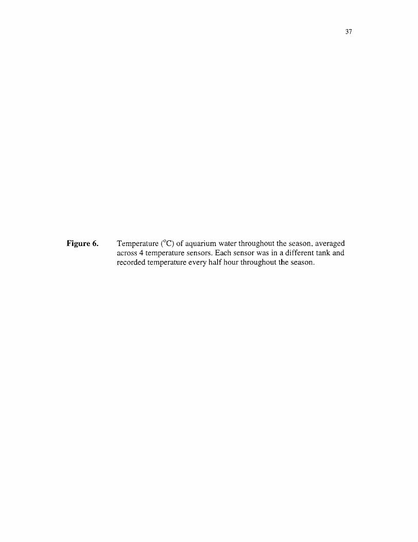
37

Figure 6. Temperature (°C) of aquarium water throughout the season, averaged across 4 temperature sensors. Each sensor was in a different tank and recorded temperature every half hour throughout the season.

Tem

pera

ture

(°

C)

30

25

20

15

10

5

0c\jCD

COOJ

COCDCO GO

Date

38

pH

Aquarium water pH was measured four times throughout the season at

approximately midday (App. 3) Mean pH was 7.7 (SE + 0.052) and did not change

appreciably throughout the season. pH decreased with increasing salinity (Table 5,

ANOVA, p<0.0001), except for the 15 psu treatment, which was greater than the 10 psu

treatment, although not significantly so (SNK>0.05). One aquarium (#28, 8% light, 10

psu salinity) had a pH of 5.04 on July 27. Water was promptly changed.

Morphology and Production

Sprouting

The incidence of tuber sprouting was determined by counting the number of

rosettes on June 14 (19 days after planting) relative to number of tubers planted. An early

sampling date was selected for analysis in order to avoid mistaking seasonal vegetative

reproduction for tuber sprouting. An average of 94.92 (SE + 5.45) tubers m' sprouted, or

53% of those planted. Sprouting incidence did not vary by treatment (p>0.05).

Leaf Elongation

Leaf length was highly dependent on salinity (Fig 7). There was a strong inverse

relationship between salinity and length (p<0.0001, Table 6). Contrast variables indicate

changes in salinity effects between each of the first six sampling dates (except for July

19) and its consecutive sampling date. Visual inspection suggests that the effects of

salinity increase over time as leaves elongate but then level out after August 16 as leaves

senesce.

39

Table 5. Mean pH per salinity treatment, with associated standard error. Seasonal means of aquariums were used for mean salinity treatment values (n=12).

Salinity (psu) Mean SE0 7.99 0.0675 7.74 0.08110 7.40 0.09415 7.54 0.058

40

Figure 7. Mean length of longest leaf per rosette over time for each light and salinity level. Longest leaves were averaged over each aquarium to obtain one value per aquarium. These values were then averaged within treatments (n=3). Error bars represent standard error.

28% Light 8% Light 2% Light

0 psu10 -

50

5 psu40 ■

30 -

20 -

£o 10 -

05 C 05 _I 50 t

10 psu40 -

20 -

50

40 - 15 psu

20 ■

CD ^ CO

Date

41

Table 6. General linearized model repeated measures ANOVA tables for various plant characteristics overtim e. Independent variables are light and salinity. n=3 for each light/salinity treatment. % Variance is the percent variation attributed to each parameter, as determined by partitioning of variance.

DF F P % Var. W ilk’s Lambda P

Leaf Length Light 2 1.03 0.3728 2.6Salinity 3 16.76 <0.0001 64.3Light * Salinity 6 0.31 0.9233 2.4Error 24 30.7Date 12 62.46 <.0001 49.9 <.0001Date * Light 24 1.53 0.0579 2.4 0.0129Date * Salinity 36 9.92 <.0001 23.8 <.0001Date * Light * Salinity 72 0.98 0.5327 4.7 0.1408Error (Date) 288 19.2

Leaf Width Light 2 3.85 0.051 14.3Salinity 3 10.35 0.0012 57.4Light * Salinity 6 0.55 0.7584 6.2Error 12 22.2Date 11 41.03 <.0001 61.1 0.048Date * Light 22 0.74 0.7898 2.2 0.1423Date * Salinity 33 1.4 0.0952 6.3 0.046Date * Light * Salinity 66 1.41 0.0487 12.6 0.145Error (Date) 132 17.9

Leaves per Rosette Light 2 0.74 0.4936Salinity 3 1.81 0.1913Light * Salinity 6 0.92 0.5073Error 14Date 11 50.55 <.0001 60.0 0.0049Date * Light 22 4.21 <.0001 10.0 0.0504Date * Salinity 33 2.04 0.002 7.3 0.332Date * Light * Salinity 66 0.86 0.762 6.1 0.3268Error (Date) 154 16.6

Rosette Density Light 2 9.04 0.0012 17.0Salinity 3 10.64 0.0001 30.1Light * Salinity 6 5.36 0.0012 30.3Error 24 22.6Time 12 32.36 <.0001 32.9 <.0001Time * Light 24 5.66 <.0001 11.5 0.0073Time * Salinity 36 4.94 <.0001 15.1 0.0004Time * Light * Salinity 72 2.64 <.0001 16.1 0.015Error(Time) 288 24.4

42

Light treatment did not have a significant effect on leaf length consistently over

time (p=0.3728). However, visual inspection of the data reveals that mid-summer, plants

in the 2 and 8% light levels produced longer leaves than the 28% light treatment,

especially for the 0 psu treatment (Fig. 7). Contrast variables support this observation and

indicate that the effects of light changed between July 4 and July 19 (p=0.0002) and

between August 8 and August 16 (p<0.0001). The interactive effects of light and salinity

also changed at these two periods (p<0.0001 and p=0.0013), supporting the observation

that mid-summer, light effects were most apparent in the 0 psu treatment.

Leaf length varied significantly over time (p<0.0001, Table 6, Fig. 7), with length

greatest in July (5.2 to 49.1 cm) and steadily declining until November (0 to 8.3 cm).

Primary causes of shortening of longest leaves in the latter part of the season were

decaying and breaking off at the distal end, and leaf senescence. Leaf senescence was

preceded by loss of chlorophyll, general decay, and/or breakage of leaf at base. The

effects of salinity varied among dates (p<0.0001). Paritioning of variance indicated that

date had the greatest effect on length, explaining 50% of the variance. The interaction

between salinity and date accounted for 23.8% of the variance, and the other interactions

had relatively minor effects. The effect of date was apparent in all light and salinity

treatments (Wilk’s test, Table 6).

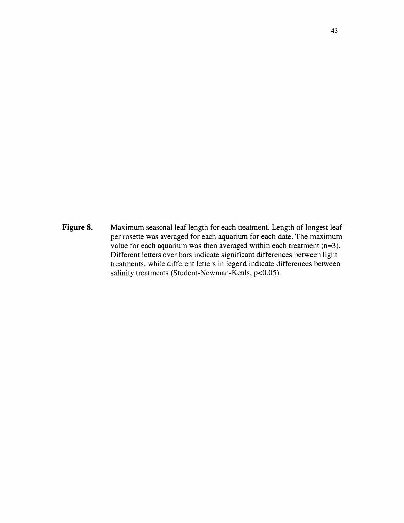
Maximum seasonal length ranged from 5.6 cm to 52.3 cm (Fig. 8). Both light

(p=0.0351) and salinity (p<0.0001) were significantly related to maximum leaf length

(Table 7). Leaves in the 28% light treatment were significantly shorter than those in the 2

and 8% light treatments (Fig. 8, SNK, p<0.05). Salinity was inversely related to length,

although 10 and 15 psu treatments were not different. Adult plants in the 0 psu, 2 and 8%

43

Figure 8. Maximum seasonal leaf length for each treatment. Length of longest leaf per rosette was averaged for each aquarium for each date. The maximum value for each aquarium was then averaged within each treatment (n=3). Different letters over bars indicate significant differences between light treatments, while different letters in legend indicate differences between salinity treatments (Student-Newman-Keuls, p<0.05).

Leng

th

(cm

)

B60

50

40

30

20

10

08


44

Table 7. 2-way ANOVA for light and salinity effects on morphology and production characteristics. n=3 for each light/salinity combination. % Variance is the percent variation attributed to each parameter, as determ ined by partitioning of variance.

DF F P % Var.Maximum Seasonal Leaf Length Light 2 3.862 0.0351 5.2

Salinity 3 36.359 <.0001 73.4Light * Salinity 6 1.301 0.2947 5.3Error 24 16.2

Initial Elongation Rate Light 2 4.042 0.0307 5.4Salinity 3 32.472 <.0001 65.2Light * Salinity 6 3.317 0.016 13.3Error 24 16.1

Leaf Width at Maximum Length Light 2 4.688 0.0191 16.7Salinity 3 3.543 0.0297 18.9Light * Salinity 6 2.018 0.1026 21.6Error 24 42.8

Maximum Seasonal Rosette Light 2 15.937 <.0001 24.8Density Salinity 3 11.864 <.0001 27.7

Light * Salinity 6 6.163 0.0005 28.8Error 24 18.7

Aboveground Biomass Light 2 7.209 0.0035 19.4Salinity 3 6.765 0.0018 27.3Light * Salinity 6 2.602 0.0437 21.0Error 24 32.3

Aboveground Biomass per Rosette Light 2 1.156 0.3323Salinity 3 2.649 0.0729Light * Salinity 6 0.770 0.6010Error 24

Belowground Biomass Light 2 7.848 0.0024 23.5Salinity 3 3.319 0.0368 14.9Light * Salinity 6 2.857 0.0303 25.7Error 24 35.9

Belowground Biomass per Light 2 3.667 0.0415 14.0Rosette Salinity 3 1.629 0.2102 8.8

Light * Salinity 6 2.997 0.0259 33.3Error 23 43.9

Aboveground to Total Biomass Light 2 0.765 0.4778Ratio Salinity 3 1.612 0.2166

Light * Salinity 6 2.057 0.1025Error 21

Leaf Area Index Light 2 9.614 0.0009 19.5Salinity 3 11.48 <.0001 34.9Light * Salinity 6 3.502 0.0125 21.3Error 24 24.3

45

Table 7 (continued).

DF F P % Var.Aboveground biomass per Leaf Light 2 0.748 0.4857Area Salinity 3 2.095 0.1314

Light * Salinity 6 0.582 0.7405Error 24

Leaf Area per Rosette Light 2 0.244 0.7858 1.1Salinity 3 4.442 0.0133 31.2Light * Salinity 6 0.975 0.4644 13.7Error 23 53.9

Leaf Length * Width Light 2 1.579 0.2269 2.6Salinity 3 31.069 <.0001 75.8Light * Salinity 6 0.445 0.8415 2.2Error 24 19.5

Tuber Density Light 2 1.652 0.2127 8.8Salinity 3 1.757 0.1822 14.0Light * Salinity 6 0.841 0.5507 13.4Error 24 63.8

Total Tuber Biomass Light 2 1.444 0.2558 8.2Salinity 3 1.607 0.214 13.7Light * Salinity 6 0.582 0.7409 9.9Error 24 68.2

46

light treatments generally reached the water surface. Light and salinity effects did not

interact (p=0.2947). The majority of the variance in length is attributable to salinity

treatment (73.4%, Table 7), while only a small fraction is due to light treatment (5.2%) or

the interactive effects of light and salinity (5.3%).

Maximum seasonal length was generally achieved between July 5 and July 19.

Date of maximum length did not consistently differ with light (p=0.3435) or salinity

treatment (p=0.6536). However, in the 2 and 8% light treatments maximum length

occurred 2 to 4 weeks later in the 5 psu treatment than in the 0 psu treatment. In the 0 psu

treatment, maximum length occurred 2 weeks later in the 28% light treatment than in the

2 and 8% light treatment.

A linear model best described elongation. Slope was determined by best-fit line

(simple linear regression, StatView, Inc.). Initial elongation rates ranged from 0.18 cm/d

to 1.24 cm/d (Fig. 9). Elongation rate followed a similar pattern to that of maximum

seasonal leaf length. Light (p=0.0307) and salinity (p<0.0001) each were significantly

correlated with elongation rate (Table 7). Plants in the 2 and 8% light treatments

elongated significantly faster than 28% light plants did, and salinity differences were

most pronounced at the lower two light levels. Elongation rate significantly decreased

with each increasing salinity level, although the difference between 10 and 15 psu

treatments was not significant (Fig. 9, SNK, p<0.05). Light and salinity effects interacted

(p=0.016). As with maximum seasonal leaf length, most of the variance was due to

salinity treatment (65.2%), while very little was attributable to light treatment (5.4%).

47

Figure 9. Mean initial leaf elongation growth rate (cm/day), measured as slope of growth curve from the start of the experiment (planting) to date of longest leaf length. Slope of line was determined for each aquarium by regression (n=3). Different letters over bars indicate significant differences between light treatments, while different letters in legend indicate differences between salinity treatments (Student-Newman-Keuls, p<0.05).

Leaf

Elo

ngat

ion

Rate

(cm

/day

)

2.0

0 psu = a 5 psu = b 10 psu = c 15 psu = c

B

28 8 2


48

Leaf Width

Throughout the course of the study width of the longest leaf per rosette decreased

with increasing salinity (p=0.0012, Table 6, Fig. 10). Light had a borderline significant

positive effect (p=0.0510), which was only apparent in the 0 and 5 psu treatments. Width

also varied significantly with time (p<0.0001). Width generally decreased throughout the

season, although it first increased to a mid-summer peak in the 0 and 5 psu, 28% light

treatments and the 5 psu, 8% light treatments. For example, in the 15 psu treatments,

average leaf width, which ranged from 2.7 to 3.3 mm in June, decreased to 0.9 to 1.8 mm

in November. In contrast, in the 0 psu, 28% light treatment leaf width increased from 4.0

to 4.8 mm from June to July and then decreased to 2.6 mm by November. The pattern for

the observed decreasing width was that the older, wider leaves senesced and were

replaced with more narrow leaves. The effects of time did not interact with the effects of

salinity (p=0.0952) or light (p=0.7898). There was no interactive effect between light and

salinity (p=0.7584), but there was between light, salinity, and time (p=0.0487).

During the period of maximum seasonal leaf length (as described above) leaf

width again decreased with increasing salinity (p=0.0297) and with decreasing light

availability (p=0.0191, Table 7, Fig. 11). Light and salinity accounted for approximately

the same amount of variance (18.9% for salinity and 16.7% for light). However, a large

portion of the variance (42.8%) could not be explained by the single or interactive effects

of light or salinity.

The product of length and width provides an approximation of shoot surface area.

Length * width at the time of maximum seasonal leaf length ranged from 1.8 to 19.2 cm .

49

Figure 10. Mean width (mm) of the longest leaf per rosette in each light and salinity treatment. Data were averaged within aquariums to yield one value per aquarium. These values were then averaged within treatments (n=3). Error bars represent standard error.

5

4

3

2

1

05

4

3

2

1

05

4

3

2

1

05

4

3

2

1

0

6/21

28% Light 8% Light 2% Light 0 psu

5 psu

10 psu

15 psu

ID 05 CJ CD 05^ ^ CO - ^

00 00 05

r - in W r - « 05 0 . 0

Date

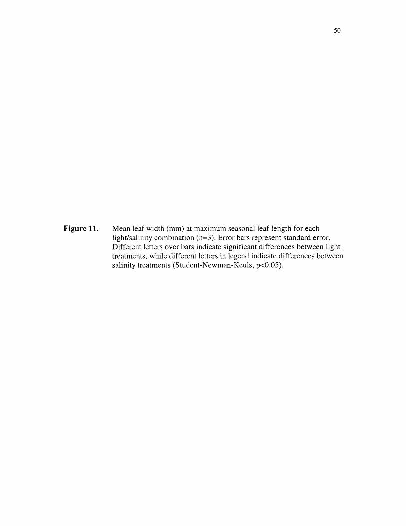
50

Figure 11. Mean leaf width (mm) at maximum seasonal leaf length for eachlight/salinity combination (n=3). Error bars represent standard error. Different letters over bars indicate significant differences between light treatments, while different letters in legend indicate differences between salinity treatments (Student-Newman-Keuls, p<0.05).

28 8 2


51

Length * width decreased with increasing salinity (pcO.OOOl) and was not related to light

(p=0.2269).

Leaf Production

Neither light nor salinity had a consistent effect on leaf production per rosette

(p>0.05, Table 6). Number of leaves per rosette did, however, vary over time (pcO.OOOl).

By mid-June, plants averaged 4.7 leaves per rosette (Fig. 12). By early July, leaf

production increased to 6.5 leaves per rosette. Leaf abundance steadily declined after that

peak, to a low of 2.9 leaves per rosette in November. The effects of time also interacted

with both light (pcO.OOOl) and salinity (p=0.002). However, these interactive effects

explained much less of the variance (10.0% for time*light and 7.3% for time*salinity)

than time alone (60.0%). The interactive effects did not exhibit any clear pattern.

Vegetative Reproduction

Rosette production varied seasonally and was highly dependent on light and

salinity treatments (Fig. 13). Averaged over all dates, vegetative reproduction increased

with increasing light (p=0.0012, Table 6). Plants in the 2% light treatment typically

produced the fewest rosettes (Fig. 13). Plants in the 28% light treatment produced

substantially more than either of the other light treatments at salinities less than or equal

to 10 psu. Salinity had a highly significant negative effect on vegetative reproduction

(p=0.0001, Table 6). Rosette abundance was highly variable throughout the season and

between treatments, ranging from 26 to 695 rosettes m~ .

52

Figure 12. Seasonal change in number of leaves per rosette, averaged across all treatments (n=36). Data were pooled because repeated measures ANOVA indicated no statistical difference between treatments (p>0.05).

# L

eave

s/ro

sett

e

2 H----------- 1 i i i i i i i i i i i

r in 05 CM <3 ^t - CM r~- ■»— T - CM T - N 3s ^1 i :CD CD ^ 0 0 0 0 0 > 0 > ® ® r -

Date

53

2Figure 13. Mean rosette density (nT ) over time for each light and salinity treatment.

Numbers of rosettes were averaged to obtain one value per aquarium. These values were then averaged across treatments (n=3). Error bars represent standard error.

700600 0 psu500

400

300

200

100

700

5 psu600 28% Light 8% Light 2% Light

500

400

300 :

200

a 7 0 0,Q)O 600 : O'

500 :

10 psu

400

300

200

100

700

600 15 psu500

400

300

200

100

l O O i <N <o <75 ^ N- *”

Date

54

There was a strong interaction of the effects of salinity and light (Table 6,

p=0.0012) such that the effects of salinity were most apparent in 28% light treatment and

the light effects were most pronounced at the 0 and 5 psu salinity levels (Fig. 13).

Partitioning of variance revealed that light accounted for 17% of variation, while salinity

accounted for 30%. The light*salinity interaction accounted for 30%, and the remainder

(23%) was not attributable to either factor.

Rosette density varied significantly over time (p<0.0001, Table 6), with density

generally highest in the middle of July and beginning of August (Fig. 13). Maximum

rosette density was also dependent on light (p<0.0001) and salinity (p<0.0001) (Table 7,

Fig. 14). Plants in the 28% light, 0 psu treatment produced a maximum of 717 rosettes

m‘ . Maximum production of plants in the low light, 15 psu treatment was the lowest, at

104 rosettes m~ . Light and salinity strongly interacted for this parameter (p=0.0005).

Loss of rosettes in the latter part of the season was due to leaf senescence and rosettes

coming loose from the sediment. The effect of date was apparent in all light and salinity

treatments (Wilk’s test, Table 6).

Rosette density increased approximately linearly from the start of vegetative

reproduction (June 14) to the approximate date of maximum density (July 19). Rosette

production in the 28% light, 0 psu treatment increased at the greatest rate, averaging a

17% increase per day over initial abundance. Rosette production in the 8% and 2% light,

0 psu treatments was 9% and 3% d '1, respectively. Growth rate of 5, 10, and 15 psu

treatments ranged from 6 to 12% d '1, 4 to 6% d*1, and 0 to 3% d’1.

55

Figure 14. Mean maximum seasonal rosette density. Numbers of rosettes per pot were converted to m-2 and then averaged for each aquarium. Maximum values were then averaged for each treatment (n=3). Different letters over bars indicate significant differences between light treatments, while different letters in legend indicate differences between salinity treatments (Student-Newman-Keuls, p<0.05).

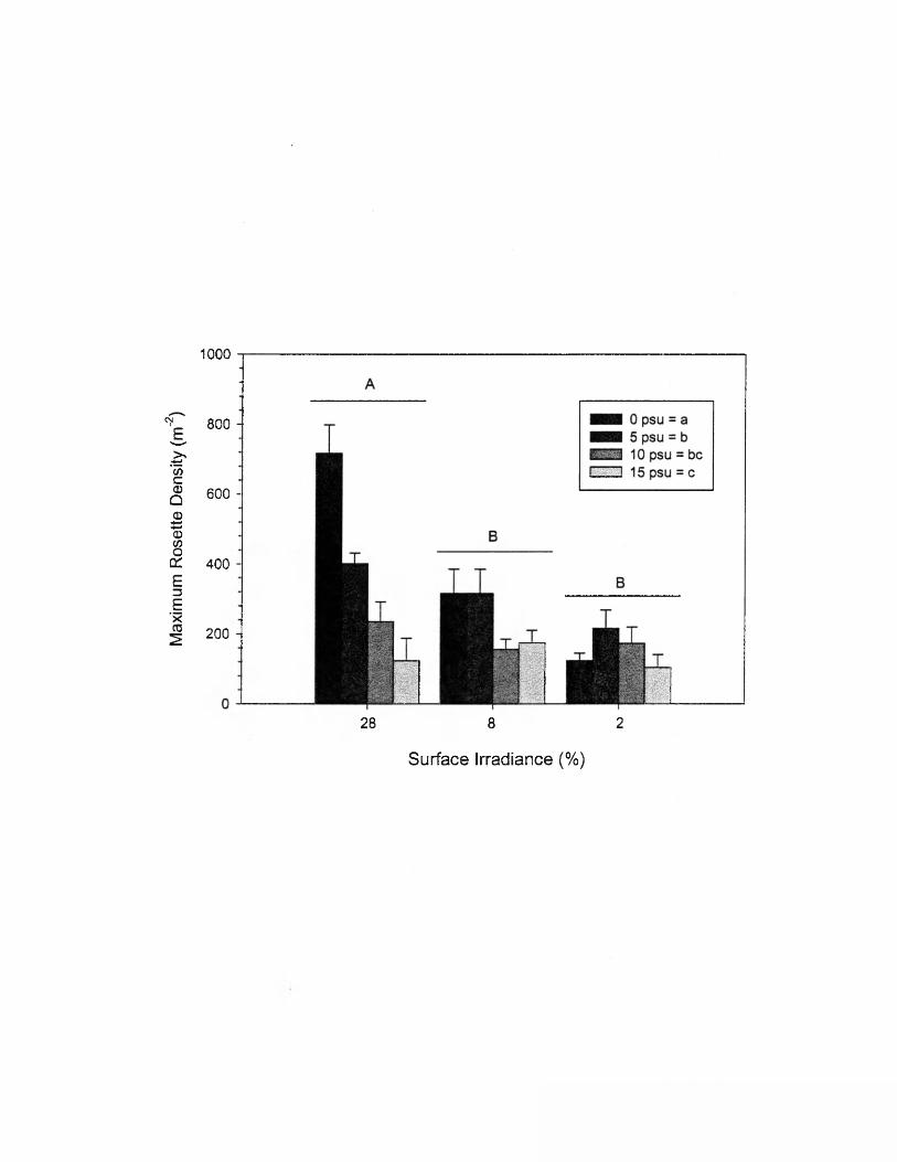
Max

imum

Ro

sette

De

nsity

(m

'2)

1000

800 -

600 -

400 -

200 -

28 8 2


56

The effects of light and salinity on rosette density varied over time, as did the

interaction between light and salinity (p<0.0001 for each). Partitioning of variance (Table

7) indicated that date alone had the greatest effect on vegetative reproduction, explaining

33% of the variance. The interactions between date and light (12%), date and salinity

(15%), and date, light, and salinity (16%) were less pronounced.

Contrast variables reveal the times at which the effects of light and salinity on

rosette production changed. A critical period was June 14 to June 21, when the effects of

light (p<0.0001), salinity (p<0.0001), and light*salinity (p=0.0002) all changed. Visual

inspection of the data (Fig. 13) indicates minimal growth prior to this period and thus

little, if any, light or salinity effects. Once rosette production increased, light and salinity

effects became pronounced. The light and salinity factors then interacted such that light

effects were most apparent at lower salinities and salinity effects were most prevalent for

the 28% light treatment.

Another critical period was July 19 to August 2, when again, the effects of light

(p=0.0021), salinity (p=0.0070), and light*salinity (p=0.0058) all changed. This two-

week period of the life history of V. americana generally marks the beginning of the

decrease in rosette density. This decrease is most apparent in the lower salinity and

higher light treatments.

The effects of salinity were more variable over time than were the effects of light.

Salinity effects changed often throughout the season. In addition to the highly significant

changes at the dates above, its effects also changed between sampling dates August 16

and 29 (p=0.0247), September 27 and October 11 (p=0.0296), and October 11 and 25

(p=0.0119).

57

Mid-Season Harvest

Biomass

Aboveground biomass was directed related to light availability (p=0.0035, Table

7, Fig. 15) and inversely related to salinity (p=0.0018). Treatment means ranged from 1.9

to 47.0 gdw m' . Aboveground biomass of plants in the 28% light treatment was

significantly greater than that of the other two light levels (SNK, p<0.05), with a trend of

greater biomass under 8% light than under 2% light. Aboveground biomass also

generally increased with decreasing salinity, with 0 and 5 psu significantly different than

10 and 15 psu (SNK, p<0.05). Light and salinity effects interacted (p=0.0437). The

effects of salinity were most apparent in the 28% light treatment, and the light effects

were only apparent at the 0 and 5 psu levels. Light explained 19% of the variance in

aboveground biomass, and salinity explained 27%. The interaction between light and

salinity accounted for 21%, and 32% of the variance was not attributable to either of the

factors (Table 7).

Examination of aboveground biomass per rosette removes the effect of vegetative

reproduction and is, therefore, a measure of shoot growth alone. Aboveground biomass

per rosette was not consistently related to light or salinity (p>0.05, Table 7, Fig. 16),

although it displayed a downward trend with increasing salinity, particularly in the 28%

light treatment. It also exhibited a downward trend with decreasing light in the 0 and 5

psu treatments.

Belowground biomass followed the same general pattern as aboveground

biomass. Treatment means ranged from 1.6 to 50.7 gdw m'2. Belowground biomass was

58

Figure 15. Mean aboveground biomass (g dry weight) per m2, of August 4 sampling (n=3). Error bars represent standard error. Different letters over bars indicate significant differences between light treatments, while different letters in legend indicate differences between salinity treatments (Student- Newman-Keuls, p<0.05).

Abo

vegr

ound

bi

omas

s (g

dry

wei

ght)

per

m

A


59

Figure 16. Mean aboveground biomass (g dry weight) per rosette from mid-season harvest, n = 3 for most light/salinity combinations. Identical letters over bars and in legend indicate no significant difference between means (Student-Newman-Keuls, p>0.05).

Abo

vegr

ound

bi

omas

s (g)

per

ros

ette

0.16

0.14

0.12

0.10

0.08

0.06

0.04

0.02

0.0028 8


60

directly related to light (p=0.0024, Table 7, Fig. 17), with biomass in the 28% light

treatment significantly greater than in the 8% or 2% light treatments (SNK, p<0.05).

Belowground biomass was inversely related to salinity (p=0.0368). The one notable

exception was the 28% light, 5 psu treatment, where the biomass was greater than in the

28%, 0 psu treatment. Plants in one aquarium contributed to the high biomass of this

treatment. The only statistically significant difference for salinity treatments was between

the 5 and 15 psu treatments. The effects of light and salinity interacted (p=0.0303), with

the effects of salinity generally more apparent in the 28% light treatment and the light

effects most apparent in the 0 and 5 psu treatments. In contrast to the aboveground

biomass response, light had more of an effect on belowground biomass than did salinity,

explaining 24% of variance compared to 15% for salinity (Table 7). The interaction

between light and salinity explained even more variance (26%), and 36% of the variance

could not be explained by either of the factors.

Belowground biomass per rosette was directly related to light (p=0.0415, Table 7,

Fig. 18), with values in the 28% light treatment significantly greater than those of the 2%

light treatment (SNK, p<0.05). This difference, however, appears to be primarily due to

the very high value of the 28% light, 5 psu treatment. Salinity did not have a consistent

effect on belowground biomass per rosette.

Aboveground-to-total biomass ratio ranged from 0.32 to 0.82 and was not

statistically different between treatments (light: p=0.4778; salinity: p=0.2166;

light*salinity=0.1025, Table 7), with no apparent trends. The aboveground-to-total

biomass ratio per rosette was also not related to light or salinity (p>0.05).

61

Figure 17. Mean belowground biomass (g dry weight) per m of August 4 sampling (n=3). Error bars represent standard error. Different letters over bars indicate significant differences between light treatments, while different letters in legend indicate differences between salinity treatments (Student- Newman-Keuls, p<0.05).

80

70

60

50

40

30

20

10

0

A

m m 0 psu = abw m i 5 psu = a

10 psu = abc n 15 psu = b

28 8 2


62

Figure 18. Mean belowground biomass (g dry weight) per rosette from mid-season harvest, n = 3 for most light/salinity combinations. Different letters over bars indicate significant differences between light treatments, while different letters in legend indicate differences between salinity treatments (Student-Newman-Keuls, p<0.05).

Belo

wgr

ound

bi

omas

s (g)

per

ros

ette

0.20

0.15

0.10

0.05

0.0028 8 2


63

Leaf Area

Leaf area followed the same general pattern as above- and belowground biomass,

although the effects of light and salinity were even more pronounced. Leaf Area Index

varied greatly between treatments (0.08 to 3.2). Light was directly related to leaf area

(p=0.0009, Table 7, Fig. 19) and accounted for 19% of variation. The 28% light treatment

produced the greatest leaf area (SNK, p<0.05), with a trend of 8% light producing greater

leaf area than 2% light. Salinity was inversely related to leaf area (p<0.0001) and

explained 35% of variation. Leaf area was greatest from low salinity to high, although

differences between 0 and 5 psu, and 10 and 15 psu were not significant (SNK). The

effects of light and salinity interacted (p=0.0125). This interaction accounted for 21% of

variation.

Aboveground biomass per leaf area, an indication of leaf thickness, was not

related to light (p=0.4857, Table 7, Fig. 20). It was also not significantly related to

salinity (p=0.1314), although there was a trend of increased thickness at higher salinity.

Leaf area per rosette was not related to light (p>0.05, Table 7, Fig. 21), but was

related to salinity (p=0.0133). Leaf area per rosette generally decreased with increasing

salinity, although the only significant difference was between 0 and 15 psu (SNK,

p<0.05).

The product of leaf length and width, a measure of leaf area per shoot (for the

longest leaf per rosette) was not significantly related to light (p>0.05, Table 7, Fig. 22)

but decreased with increasing salinity (p<0.0001).

64

9 9Figure 19. Mean leaf area (cm per cm sediment surface) of mid-season sampling (n=3). Error bars represent standard error. Different letters over bars indicate significant differences between light treatments, while different letters in legend indicate differences between salinity treatments (Student- Newman-Keuls, p<0.05).

Leaf

Are

a (c

m2/c

m2 s

edim

ent

surf

ace)


65

2Figure 20. Aboveground biomass/leaf area (mg/cm ), an indication of leaf thickness,

from mid-season harvest. n=3 for most light/salinity combinations. Identical letters over bars and in legend indicate no significant difference between means (Student-Newman-Keuls, p>0.05)

Abo

vegr

ound

bi

omas

s/le

af a

rea

(mg/

cm2)

28 8 2


66

'yFigure 21. Mean leaf area (cm ) per rosette from mid-season harvest. n=3 for most

light/salinity combinations. Different letters over bars indicate significant differences between light treatments, while different letters in legend indicate differences between salinity treatments (Student-Newman-Keuls, p<0.05).

100

90

80

70

60

50

40

30

20

10

0


67

Figure 22. Mean length * width (cm2) at maximum seasonal leaf length for each light/salinity combination (n=3). Error bars represent standard error. Different letters over bars indicate significant differences between light treatments, while different letters in legend indicate differences between salinity treatments (Student-Newman-Keuls, p<0.05).

Leng

th*W

idth

(c

m2)

25

20 -

15 -

10 -


Reproductive Structures

Flowering was observed in August and September and was observed in only 6

aquariums, all in 28 or 8% light and 0 or 5 psu treatments (App. 4). Most flowering plants

produced seeds later in the season.

Tubers were harvested on December 13, several weeks after winter dieback. Only

firm tubers with no evidence of decomposition were counted. Tuber production by

treatment ranged from 66 to 500 tubers m' (Fig. 23). Tuber production was variable

within treatments and so was not significantly related to light (p=0.2127, Table 7) or

salinity (p=0.1822). However, there is a clear trend of increasing tubers with increasing

light and also with decreasing salinity. Salinity effects were most apparent at 28 and 8%

light, and light effects were most prominent at 0 psu. The ratio of end-of-season tubers to

maximum seasonal rosettes (Fig. 23) ranged from 0 to 2.2 tubers/rosette by aquarium

(mean 0.65, SE + 0.096) and did not differ by treatment (p>0.05, Table 7).

Individual tuber biomass was 0.019 gdw (SE + 0.002) and was not related to light

or salinity (p>0.05). Total tuber biomass m' also was not significantly related to light

(p=0.2558, Table 7, Fig. 23) or salinity (p=0.2140), but displayed a similar trend to that

of number of tubers produced.

Photosynthesis

Chlorophyll

Leaves were collected for chlorophyll a and b analysis on July 6, August 2,

September 1 and September 29. Statistical analyses of July 6 and August 2 data are

69

Figure 23. Mean number and biomass of tubers (g dry weight) m '2 harvested at the end of the growing season. n=3 for each light/salinity combination. Identical letters over bars and in legend indicate no significant difference between means (Student-Newman-Keuls, p>0.05).

A

800

Ee0

-Q13

600

400

200

0

25

- CQ)02?

T3

30CO03Eolot—0-QD

20

15

10

28

■ ■ ■ 0 psu = a umuw 5 psu = a

10 psu = a 15 psu = a


70

presented below. Data obtained from September 1 samples were lost due to analytical

problems. Due to plant dieback, September 29 sample size was too small for ANOVA

analysis (n=21).

For July 6 samples, chlorophyll a concentrations ranged from 0.60 to 1.93

mg/dm2 and decreased with increasing light (p<0.0001, Table 8, Fig. 24). Chlorophyll a

concentrations were also significantly related to salinity (p=0.0321), although the only

significant difference was between 0 psu and 10 psu treatments, and there was only a

trend of increasing concentrations with increasing salinity. Chlorophyll b concentrations

ranged from 0.46 to 1.11 mg/dm and also decreased with increasing light (p=0.0001,

Table 8, Fig. 24), with concentration of plants in the 2% light treatment significantly

greater than those in the 8% and 28% light treatments (SNK, p<0.05). Salinity did not

have a consistent effect (p=0.1041). The ratio of chlorophyll a to chlorophyll b

concentration was also inversely related to light (p=0.0021, Table 8, Fig. 24), with

chlorophyll a:b of plants in the 2 and 8% light treatments (1.75 to 2.11) greater than that

in the 28% light treatment (1.20 to 1.54) (SNK, p<0.05). Salinity did not have a

consistent effect on the ratio of chlorophyll a to b (p=0.4712).

August 2 samples displayed similar chlorophyll patterns. Chlorophyll a

concentration ranged from 0.49 to 2.04 mg/dm and decreased with increasing light

(p=0.0024, Table 8, Fig. 25), with the chlorophyll concentration of plants in the 2% light

treatment greater than that in the 8 or 28% light treatment (SNK, p<0.05). Chlorophyll a

concentration was not, however, related to salinity (p=0.2746). Chlorophyll b

concentration ranged from 0.39 to 1.16 mg/dm2 and followed the same pattern as that of

71

Table 8. 2-way ANOVA results for light and salinity effects on chlorophyll concentrations and chlorophyll a/b ratios. n=3 for each light/salinity combination. % Variance is the percent variation attributed to each parameter, as determined by partitioning of variance.

DF F P % Var.Chlorophyll a, July 6 Light 2 16.435 <.0001 46.5

Salinity 3 3.46 0.0321 14.7Light * Salinity 6 0.57 0.7502 4.8Error 24 34.0

Chlorophyll b, July 6 Light 2 13.1 0.0001 42.5Salinity 3 2.289 0.1041 11.1Light * Salinity 6 0.762 0.6065 7.4Error 24 38.9

Chlorophyll a/b, July 6 Light 2 8.079 0.0021 36.2Salinity 3 0.868 0.4712 5.8Light * Salinity 6 0.307 0.927 4.1Error 24 53.8

Chlorophyll a, August 2 Light 2 7.906 0.0024 31.8Salinity 3 1.378 0.2746 8.3Light * Salinity 6 1.137 0.3729 13.7Error 23 46.2

Chlorophyll b, August 2 Light 2 9.979 0.0008 35.6Salinity 3 1.919 0.1546 10.3Light * Salinity 6 1.228 0.3283 13.2Error 23 41.0

72

Figure 24. Mean chlorophyll a and b (mg/dm ) and chlorophyll a/b ratio of leaf tissue harvested on July 6. One leaf was collected per aquarium (n=3). Error bars represent standard error. Different letters over bars indicate significant differences between light treatments, while different letters in legend indicate differences between salinity treatments (Student-Newman-Keuls, p<0.05).

July 6

2.5

CM

E;oO)E,CD

2.0

1.5>szCLOL_oszO

1.0

0.5

0.0

O

1.5

EO)E 1.0

szClO 0.5

0.0

3.0 T0 psu = a 5 psu = a 10 psu = a

28 8 2


73

Figure 25. Mean chlorophyll a and b concentrations (mg/dm2) of leaf tissue harvested on August 2. One leaf was collected per aquarium (n=3). Error bars represent standard error. Different letters over bars indicate significant differences between light treatments, while different letters in legend indicate differences between salinity treatments (Student-Newman-Keuls, p<0.05).

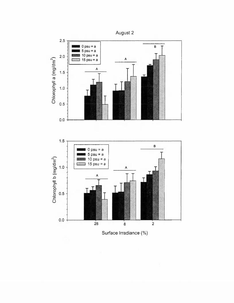
Chl

orop

hyll

b (m

g/dm

2) C

hlor

ophy

ll a

(mg/

dm2)

August 2

2.5

2.0

1.5

1.0

0.5

0.0

warn 0 psu = amom 5 psu = al:-: '1 10 psu = aL— J 15 psu = a

28 8 2


74

chlorophyll a , with concentration in the 2% light treatment greater than that in the 8 or

28% light treatment (Table 8, Fig. 25, SNK, p<0.05). Again, chlorophyll b concentration

was not related to salinity. The ratio of chlorophyll a to b concentrations was not related

to light (p=0.155) or salinity (p=0.4741).

September 29 samples exhibited a trend of higher chlorophyll a and b

concentrations in the 8% light treatment (Fig. 26). This pattern was driven primarily by a

decrease in chlorophyll a concentration from July 6 and August 2 levels in the 2% light

treatment and an increase in chlorophyll b concentration from earlier levels in the 8%

light treatment.

PAM Fluorometry

Quantum Yield

Due to plant dieback throughout the season, there were too many missing

quantum yield data (App. 5) to conduct repeated measures ANOVA, even when

employing the general linear model for imbalanced design. There were still insufficient

data when the last two dates were eliminated from analysis, at which time half the

aquariums no longer had plants (The SAS® System for Windows, SAS Institute Inc.).

Three-way ANOVA was conducted instead, with date as a factor, in addition to light and

salinity, to quantify treatment effects. Due to small sample size on September 29 (n=16),

this sampling date was eliminated from the effective and maximal quantum yield

analyses.

75

2Figure 26. Chlorophyll a and b concentrations (mg/dm ) of leaf tissue harvested on

September 29. One leaf was collected per aquarium (n=3). Sample size is less than three for some treatments due to plant dieback. Error bars represent standard error.

2.5

September 29

CM

ETDO)E,CO

>»-CQ .2oszO

2.0 -

mam 0 psumam 5 psu

FT"!10 psu 15 psu

1.5


76

Effective Quantum Yield

Effective quantum yield ranged from 0.61 to 0.75 at the start of the sampling

season. Light had a strong negative impact on effective quantum yield throughout the

season (p<0.0001, Table 9, Fig. 27), and explained 23% of variance, more than salinity or

any interactive effects. Plants in the 28% light treatment had the lowest effective quantum

yield (SNK, p<0.05), with yields of plants in the 8% and 2% treatments not significantly

different. Effective quantum yield was significantly related to salinity (p=0.0002), but

only 5% of the variance was attributable to this factor. Plants in the 5 psu treatment had

the highest effective quantum yield, followed by 10 psu, 0 psu, and 15 psu. Effective

quantum yield varied significantly over time (p<0.0001). Seasonal effects explained 19%

of variance. In general, effective quantum yield was lowest in August, especially for

plants in the 28% light treatment. This decline in quantum yield coincided with start of

seasonal dieback. Effective quantum yields of the 8% and 2% light, 0 and 5 psu plants

largely recovered by the end of August (0.56 to 0.74), while effective quantum yields of

plants in the other treatments recovered only partially, if at all (minimum of 0.25). The

effects of salinity and light interacted (p=0.0128), although no clear pattern emerged. The

effects of light and date also interacted (p=0.0019), with light effects generally greatest in

August and September. A large portion (33%) of variance was unexplained by single or

interactive effects of light, salinity, or date.

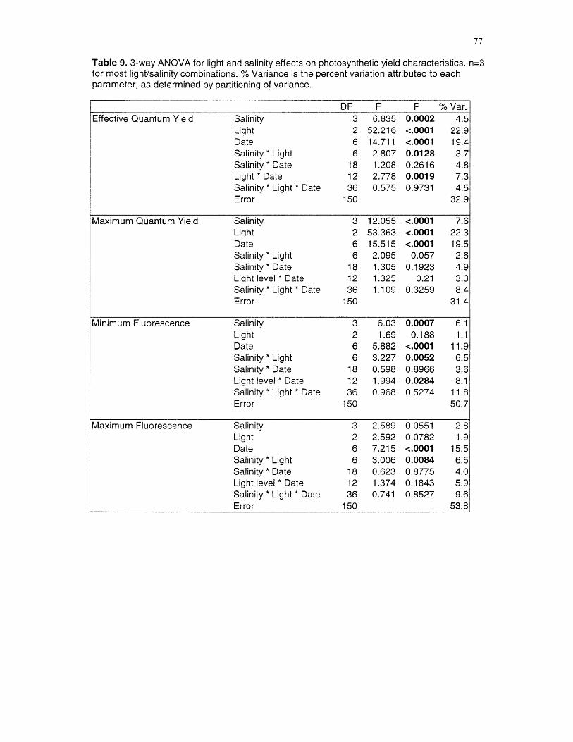
77

Table 9. 3-way ANOVA for light and salinity effects on photosynthetic yield characteristics. n=3 for most light/salinity combinations. % Variance is the percent variation attributed to each parameter, as determined by partitioning of variance.

DF F P % Var.Effective Quantum Yield Salinity 3 6.835 0.0002 4.5

Light 2 52.216 <.0001 22.9Date 6 14.711 <.0001 19.4Salinity * Light 6 2.807 0.0128 3.7Salinity * Date 18 1.208 0.2616 4.8Light * Date 12 2.778 0.0019 7.3Salinity * Light * Date 36 0.575 0.9731 4.5Error 150 32.9

Maximum Quantum Yield Salinity 3 12.055 <.0001 7.6Light 2 53.363 <.0001 22.3Date 6 15.515 <.0001 19.5Salinity * Light 6 2.095 0.057 2.6Salinity * Date 18 1.305 0.1923 4.9Light level * Date 12 1.325 0.21 3.3Salinity * Light * Date 36 1.109 0.3259 8.4Error 150 31.4

Minimum Fluorescence Salinity 3 6.03 0.0007 6.1Light 2 1.69 0.188 1.1Date 6 5.882 <.0001 11.9Salinity * Light 6 3.227 0.0052 6.5Salinity * Date 18 0.598 0.8966 3.6Light level * Date 12 1.994 0.0284 8.1Salinity * Light * Date 36 0.968 0.5274 11.8Error 150 50.7

Maximum Fluorescence Salinity 3 2.589 0.0551 2.8Light 2 2.592 0.0782 1.9Date 6 7.215 <.0001 15.5Salinity * Light 6 3.006 0.0084 6.5Salinity * Date 18 0.623 0.8775 4.0Light level * Date 12 1.374 0.1843 5.9Salinity * Light * Date 36 0.741 0.8527 9.6Error 150 53.8

78

Figure 27. Mean effective yield for light and salinity treatments over time. Error barsare standard error for a maximum of 3 samples. Sample size is less than 3on some dates due to insufficient leaf material.

20ye3cCO=3

ao>o

sSLU

0.8 7----*

0.6

0.4


0.2 0 psu

0.00.8

5 psu

0.0

10 psu

0.8

0.6

0.4

0.215 psu

0.0CMCM

00CO CM00 05 Ol00

Date

79

Effective quantum yield of plants in the 28% light, 0 psu treatment was low by the

Aug 2 sampling date (0.45, Fig. 27) due to very low effective quantum yields of plants in

two of the three aquariums. Leaves of these plants had become very thin, pale, and brown

by this time.

Maximal Quantum Yield

Initial maximal quantum yield ranged from 0.62 to 0.77. Similar to effective

quantum yield, light had a strong negative effect on maximal quantum yield (p<0.0001,

Table 9, Fig. 28) and explained 22% of variance. Maximal quantum yield of plants in the

28% light treatment was significantly lower than that of the other two light treatments

(SNK, p<0.05). Maximal quantum yield in the 8% light treatment was generally lower

than that in the 2% treatment, although not significantly so. Salinity also had a significant

effect on maximal quantum yield (p<0.0001), although it only explained 8% of variance.

The maximal quantum yield of plants in the 15 psu treatment (minimum of 0.33) was

significantly lower than that of any of the other three treatments (SNK, p<0.05),

particularly at high light. Maximal quantum yield was next lowest in the 0 psu treatment,

followed by the 10 psu treatment. Maximal quantum yield was highest in the 5 psu

treatment, although it was not significantly greater than in the 10 psu treatment. Maximal

quantum yield varied significantly over time (p<0.0001). Date explained 19% of

variance. Although the pattern was not as great as for effective quantum yield, maximal

quantum yield tended to decrease in August. This parameter partially or fully recovered

by the end of September for plants in the 2 and 8% light, 0 and 5 psu treatments. None of

80

Figure 28. Mean maximal quantum yield for light and salinity treatments over time.Error bars are standard error for a maximum of 3 samples. Sample size isless than 3 on some dates due to insufficient leaf material.

0.8

0.6 -1

0.4

0.228% Light

- o - 8% Light -T - 2% Light

0 psu

10 psu

0.8

0.6

0.4

0.215 psu

0.0CO o>

CN05

CMCMCO

CMCM

CO05 0500

Date

81

the interactions between factors was significant (p>0.05). A large portion of variance

(33%) was unexplained by any of the factors or their interactions.

Minimum Fluorescence

Initial minimum fluorescence (Fo), determined from dark-adapted leaves, ranged

from 175 to 483 mV. Salinity had a significant effect on Fo (p=0.0007, Table 9, Fig. 29).

It followed roughly the opposite pattern as that of effective and maximal quantum yield,

with Fo highest in the 15 psu treatment, followed by the 10, 0, and 5 psu treatments. F0 in

the 15 and 10 psu treatments was significantly greater than that in the 5 and 0 psu

treatments (SNK, p<0.05). Salinity, however, accounted for only 6% of total variance.

Light did not have a significant effect on Fo (p>0.05). Date was significantly related to Fo

(p>0.0001) and accounted for the most variance of the three factors (12%). Fo generally

increased throughout the season. The effects of salinity and light (p=0.0052), as well as

salinity, light, and date (p=0.0284), interacted. The majority of variance (51%), however,

was unexplained by any of the three factors or their interactions.

Maximum Fluorescence

Initial maximum fluorescence (Fm) ranged from 641 to 1461 mV. Salinity did not

have a significant effect on Fm (p=0.0551, Table 9, Fig. 30), although there was a trend of

Fm in the 10 and 15 psu treatments exceeding Fm in the 0 and 5 psu treatments. Light did

not significantly affect Fm (p=0.0782). Date did, however, have a highly significant

82

Figure 29. Mean minimum fluorescence for light and salinity treatment over time.Error bars are standard error for a maximum of 3 samples. Sample size isless than 3 on some dates due to insufficient leaf material.

1000


800 -

600 -

400 -

200 - 0 psu

1000

800 -

600 ->& 400 -0| 200-o <n2 0 j § 1000 f

LL

E 800 -=3Ec 600 -

5 psu

400 -

200 - 10 psu

1000

800 -

600 -

400 - 15 psu

200 -

CO 05CM05

CMCMCM

CMCO

0505CO

Date

83

Figure 30. Mean maximum fluorescence for light and salinity treatments over time.Error bars are standard error for a maximum of 3 samples. Sample size isless than 3 on some dates due to insufficient leaf material.

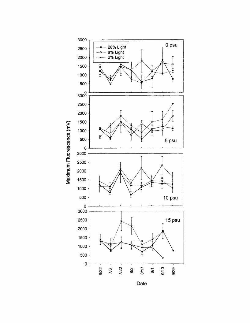
>E,0Oc0OCOs>o_d

LI_

EDEx0

30000 psu28% Light

8% Light 2% Light

2500 ■

2000 -

1500 -

1000 -

500 -

2500 -

2000 -

1500 -

1000 -

500 - 5 psu

3000

2500 -

2000 -

1500 -

1000 -

500 - 10 psu

3000

15 psu2500 -

2000 -

1500 -

1000 -

500 -

S se 8CD ^ l »

C\l00

^ r-5 55

00'T”05

05CN05

Date

effect (pcO.OOOl) and explained 16% of variance. The effects of salinity and light

interacted (p=0.0084), but the others did not. As with Fo, the three treatment factors and

their interactions accounted for little of the total variance, with 53% of variance

unexplained.

Rapid Light Curves

Rapid light curves were generated on August 20 (Fig. 31), September 12 (Fig.

32), October 3, and Oct 20. One light curve was conducted per aquarium that had plants

(App. 5). Because of limited sample size on October 3 (n=18) and October 20 (n=13),

these dates were excluded from analysis.

Maximum ETR (determined here as the average of the three highest consecutive ETRs

per light curve) is an indication of photosynthetic capacity. ETRmax was directly related to

light availability on August 20 (p=0.0017, Table 10, Fig. 33). ETRmax in the 28% light

treatment was significantly higher than that in the 8% or 2% light treatment (SNK,

p<0.05, Fig. 33). Salinity did not significantly affect ETRmax (p=0.0919), although

ETRmax in the 28% light, 0 psu treatment was greater than that in any other light or

salinity treatment. Light explained 34% of variance, and 33% was not attributable to

these factors.

The minimum saturating irradiance (Ik) varied by light treatment. Ik in the 28%

light treatment was significantly greater than Ik in the 8 or 2% light treatments (p=0.0024,

Table 10, Fig. 34). Light explained 39% of variance. Salinity did not have a consistent

effect on Ik. A large portion (41%) of variance was unexplained by light or salinity or

their interaction.

85

Figure 31. Rapid light curves on August 20. Sample size is 3 for most light/salinity combinations. It is less than 3 for several treatments due to insufficient leaf material. Error bars represent standard error.

CO

(/)c2 -t—<o00

OE

q:h—UJ

60 -

50 -

40 -

30 -

20 - 28% Light 8% Light 2% Light10 -

60 - 5 psu50 -

40 -

30 -

20 -

10 -

60 -10 psu

50 -

40 -

30 -

20 -

10 -

60 - 15 psu50 -

40 -

30 -

20 -

10 -

2500200015001000500

PAR

86

Figure 32. Rapid light curves for light and salinity treatments on September 12.Sample size is 3 for most light/salinity combinations. It is less than 3 for several treatments due to insufficient leaf material. Error bars represent standard error.

80

60

40

20

080

60'coN£ 40c/>c

00 o1 80(Zt 60

40

20

080

60

40

20

00 500 1000 1500 2000 2500

PAR

0 psu


5 psu

10 psu

15 psu

’ — — — - 4

87

Table 10. 2-way ANOVA of light and salinity effects on ETRmax and lk. n=3 for most light/salinity combinations. % Variance is the percent variation attributed to each parameter, as determined by partitioning of variance.

DF F P % Var.ETRmax, August 20 Light 2 9.33 0.0017 34.1

Salinity 3 2.504 0.0919 13.7Light * Salinity 6 1.771 0.1619 19.4Error 18 32.8

Ik, August 20 Light 2 8.564 0.0024 73.7Salinity 3 1.024 0.4052 8.8Light * Salinity 6 1.031 0.4372 8.9Error 18 8.6

ETRmax, September 12 Light 2 4.36 0.0276 22.2Salinity 3 1.413 0.2697 10.8Light * Salinity 6 1.235 0.3325 18.8Error 19 48.3

88

Figure 33. Mean maximum electron transport rate (ETRmax) for each treatment on August 20 and September 12. Maximum ETR is the average of the three highest points on a rapid light curve. Sample size is 3 for most light/salinity combinations. It is less than three for several treatments due to insufficient leaf material. Error bars represent standard error. Different letters over bars indicate significant differences between light treatments, while different letters in legend indicate differences between salinity treatments (Student-Newman-Keuls, p<0.05).

A100

80

60

40

CN 20Ew c2 oO 0 Q28CD

oE

£ 100E

O' h- LU 80

60

40

20

28 8 2


August 20

September 12A

89

Figure 34. Mean minimum saturating irradiance (Ik) for each treatment on August 20.Sample size is 3 for most light/salinity combinations. It is less than 3 for several treatments due to insufficient leaf material. Error bars represent standard error. Different letters over bars indicate significant differences between light treatments, while different letters in legend indicate differences between salinity treatments (Student-Newman-Keuls, p<0.05).

1000r \

mm o psu = a800 - BOH 5 psu = a

jgasa 10 psu = aC/3

C N^ ..' ...I 15 psii = a

28 8 2


90

The initial slope of the rapid light curve (a) was not significantly affected by light

or salinity (p>0.05).

Maximum ETR was also directly related to light on September 12 (p=0.0276,

Table 10, Fig. 32). Again, ETRmax in the 28% light treatment was significantly higher

than that in the 8% or 2% light treatment (SNK, p<0.05, Fig. 32). Salinity did not have a

significant effect on ETR,nax (p=0.2697), although in the 28% light treatment ETRmax was

much lower at 15 psu than at the other three salinity levels. Light explained 22% of

variance, and 48% was not explained by light, salinity, or their interaction.

Summary

The effects of light and salinity and their interaction on major plant characteristics

are summarized in Table 11.

91

Table 11. Summary of the effects of light and salinity and their interaction on major plant characteristics. +, factor was positively related to characteristic; factor was negatively related; X, no relationship, or no interactive effect; I, light and salinity effects interacted; *, no significant relationship, but strong trend in direction indicated.

Light Salinity InteractionMorphology

Length - - XWidth + - X# Leaves X X X

ProductionVegetative Growth + - IAboveground Biomass + - IBelowground Biomass + - ILeaf Area + - I

PhotosynthesisChlorophyll - X XQuantum Yield - - XETRmax + X X

ReproductionFlowering +* ★ XTuber Production +* ★ X

92

DISCUSSION

Morphology and Production

Salinity and Light Stress

Although both light and salinity markedly influenced V. americana production,

salinity exerted a stronger control for the ranges considered. This suggests that salinity

may control distribution of V. americana more than light availability. Upper salinity

tolerance was between 5 and 10 psu, while light tolerance was between 28 and 8% of

surface irradiance. The relatively small effect of light is likely due in large part to

morphological and photosynthetic adaptations to low light, such as increased elongation

and photochemical efficiency. In contrast, the morphological and photosynthetic

responses to salinity, such as reduced elongation and photochemical efficiency, appeared

to compound salinity stress.

Production (as defined by vegetative reproduction, above- and belowground

biomass, and leaf area index) decreased dramatically at higher salinity levels (Fig. 13, 14,

15, 17, 19). For instance, at 28% light aboveground biomass, leaf area index, and

maximum seasonal rosette production at 15 psu were 4%, 2%, and 17%, respectively, of

that at 0 psu. Overall, production was generally greatest in the 0 psu treatment, moderate

at 5 psu, and minimal at 10 and 15 psu.

The deleterious effects of elevated salinity on the production of V. americana are

well known. Although measurements of the morphology and production of naturally

existing populations of V. americana in different light and salinity regimes are generally

93

lacking, many mesocosm and transplanting studies have examined these characteristics.

For instance, Staver (1986) found that aboveground biomass of transplanted adults at 6

psu was 10% of that at 0 psu, while belowground biomass at 6 psu was 12% of that at 0

psu. Haller et al. (1974) found death at 13.32 and 16.65 psu and survival but no net

growth at 6.66 and 10.00 psu. In a transplanting field study Kraemer et al. (1999)

observed smaller plants at two sites with salinities ranging seasonally from 7 to 20 psu, as

compared to lower salinity sites, and death at another site with salinity exceeding 20 psu.

In a field study of the Pamlico River estuary, Davis and Brinson (1976, in Twilley and

Barko 1990) found V. americana present in 78.1 % of quadrats sampled in a region of

mean salinity 5.3 psu. No V. americana was present in a region with a mean salinity of

7.6 psu. These findings support the upper salinity tolerance of 5 to 10 psu determined the

current study.

Contrary to these observed patterns, Twilley and Barko (1990) found no

difference in total biomass or vegetative reproduction between plants transplanted for 5

weeks into salinities ranging from 0 to 12 psu. They attribute this high salinity tolerance

to their methodology of gradually raising salinity levels, thus enabling some

osmoregulatory mechanism to operate. It is also likely that these plants could flourish in

higher salinities in the short term only, particularly because these adult plants likely had

stored C reserves. The results of their study (i.e., salinity tolerance greater than 12 psu),

then, are more applicable to short-term salinity changes on established populations,

whereas the results of the present study are more applicable to recruitment, colonization,

and longer-term survival.

94

Reduced irradiance also stunted production. For example, in the 0 psu treatment

aboveground biomass, leaf area index, and maximum seasonal rosette density at 2% light

were 9%, 21%, and 17%, respectively, of that at 28% light. There was generally a trend

of lower production in the 2% light treatment than in the 8% light treatment, but there

was no significant difference between 2 and 8% light treatments for any of these

characteristics. The reduction in production at lower light levels indicates that light was

limiting at the 2 and 8% levels.

Reduced irradiance has been found to decrease V. americana production in

several other studies. Biomass and rosette production decreased with decreasing light at

2 11500, 600, and 100 pmol irf s' (approximately equivalent to 75, 30, and 5% light)

(Barko et al. 1982) and 550 and 125 pmol m'2 s '1 (50% and 8% light) (Barko et al. 1991).

Blanch et al. (1998) found a decrease in total number of leaves and leaf area index with

decreasing light over a wide range of light levels for plants transplanted to a pond.

Similarly, biomass and rosette production increased dramatically for transplants in

embayments when the areas were artificially illuminated (Carter et al. 1996). Twilley and

Barko (1990), however, again found no differences between biomass or rosette

production at 8% versus 50% light, likely due to the short duration of the study and to the

relatively high irradiance of even the lower light level.

Based on the results of the present study alone, it is unknown whether the 28%

light level was saturating. However, the results of several other studies suggest that this

light level was saturating. For instance, aboveground biomass increased approximately

43% from 8 to 28% light (at 0 psu) in the present study, whereas in the study by Barko et

al. (1991) it increased to a similar degree (44 to 53%, depending on nutrient and DIC

95

levels) from 8 to the higher level of 50% light. In the study by Barko et al. (1982)

aboveground biomass was not consistently higher at 75 versus 30% light. In fact, it was

lower at 75% light when grown at 24 and 28°C and only increased with increasing light

at 32°C. Rosette density was higher at 75 versus 30% light only at 28 and 32°C. The

maximum temperature achieved in the present study was 28°C; thus, it is unlikely that

growth here would have increased substantially at higher light levels.

Light and salinity levels strongly influenced not only plant production but also

morphology, which in turn altered the plants’ ability to capture available light. As with

production, salinity impacted morphology (as defined by length, width, and leaf

production per rosette) to a larger degree than did light. Leaves of high salinity plants

were shorter and narrower than those in lower salinity (Fig. 7, 8, 10, 11) and thus had less

leaf area over which to capture light (Fig. 21, 22). For instance, at 28% light surface area

per leaf in the 15 psu treatment was only 13% of that in the 0 psu treatment. Staver

(1986) also found a lower surface area per leaf at higher salinity: leaf area at 6 psu was

28% of that at 0 psu. The reduced ability to capture light due to less leaf area was

compounded by the shorter canopy height of the higher salinity treatments. Similar to the

pattern for production, leaf length and width were greatest at 0 psu, moderate at 5 psu,

and minimal at 10 and 15 psu.

In contrast to salinity stress, reduced light resulted in taller leaves, enabling more

effective light capture. Plants in the 2 and 8% light treatments were up to 66% taller than

those in the 28% treatment. Leaf elongation is a common response to low light for V.

americana (Barko et al. 1982, Barko et al. 1991), as well as other SAV species (Stross

1979, Barko and Smart 1981, Barko et al. 1982). The elongation capacity of V.

96

americana may confer a competitive advantage over certain other freshwater macrophyte

species with more limited elongation ability, such as Potamogeton nodosus (Barko et al.

1982). However, it is not a canopy-former like Hydrilla verticillata or Myriophyllum

spicatum and so generally cannot successfully compete with these species (Haller and

Sutton 1975, Titus and Adams 1979).

Although leaf lengths in the 2 and 8% light treatments were not statistically

different, length under 8% light was longer at mid-season than that in 2% light for all but

the 0 psu treatment. These results suggest that elongation capacity is diminished at some

level of irradiance below 8% surface irradiance, particularly when plants are under

salinity stress. This reduced leaf elongation effectively increased the optical depth, or

distance between the water surface and leaf surface, thereby compounding the effect of

turbidity, especially in shallow water areas.

Leaf width increased with increasing light, particularly mid-season (Fig. 10, 11).

The contrary responses of length and width to light resulted in approximately the same

surface area per leaf (measured as length * width) under reduced light, but a greater

proportion of leaf surface area near the water’s surface. Barko et al. (1982) also found no

difference in surface area per leaf between 5 and 30% light treatments. However, surface

area per leaf at 75% light was reduced. Lower light plants in the present study appeared

to shift resources away from vegetative reproduction, biomass, and total leaf area to

elongation. Thus, light stress, unlike salinity stress, elicited a response that maximized

light capture per unit of production. Therefore, the phenotypic plasticity in response to

light, in contrast to salinity, may be considered adaptive, as it appears to facilitate V.

97

americana survival in a variety of environments. In addition, it may contribute to the

species’ wider tolerance to light, relative to salinity.

Unlike leaf length or width, leaf production per rosette was not affected by light

or salinity (Fig. 12), indicating that it was neither negatively impacted by higher salinity,

nor used by low light plants as a means to increase light capture. Because this

characteristic is not generally studied, it is unknown whether its lack of plasticity to

stressors is typical. It appears to be primarily under seasonal control, with a mid-season

peak of 6.5 leaves per rosette and an end-of-season minimum of 2.9 leaves per rosette.

The impact of light on aboveground biomass was primarily through new rosette

formation, as aboveground biomass per rosette was not strongly affected by light

availability (Fig. 16). The absence of strong light effects on aboveground biomass per

rosette, coupled with the lack of effects on surface area per leaf (Fig. 22) and leaf

production per rosette (Fig. 12) suggests that leaf thickness also was not substantially

affected by light. This conclusion is supported by the lack of relationship between light

and the ratio of aboveground biomass to leaf area (Fig. 20). However, rosette size (leaf

surface area and biomass per rosette) may have been constrained by nutrients or pot size

in this study.

Contrary to these results, Blanch et al. (1998) found leaf thickness to decrease

with decreasing light. The authors suggested that the resulting increase in surface area to

volume ratio may have allowed lower light plants to intercept more light. However,

without measurements of chlorophyll concentrations, the accuracy of this statement is

unknown.

98

Although length * width per leaf (Fig. 22) and leaf area per rosette (Fig. 21) both

increased with decreasing salinity, aboveground biomass per rosette only displayed a

nonsignificant trend of higher values at lower salinity. The absence of a significant

relationship between aboveground biomass per rosette and salinity may be partially due

to a counteracting trend of leaf thickness increasing with increasing salinity (Fig. 20).

Thicker leaves minimize the surface area to volume ratio, and, thus, ion exchange, and so

may be an adaptation to salinity stress.

Belowground biomass was the only morphological or production characteristic

more controlled by light than by salinity (Fig. 17). As with aboveground biomass, salinity

induced changes to belowground biomass primarily through rosette production. Light,

however, induced changes through both rosette production and through increased growth

per rosette (Fig. 18). The decreasing belowground biomass per rosette with decreasing

light suggests that low light plants minimized belowground material in order to maximize

photosynthetic material. However, the pattern of decreasing belowground biomass per

rosette with decreasing light was primarily driven by the 28% light, 5 psu treatment, and

the ratio of aboveground to total biomass was not significantly different across light or

salinity levels. Barko et al. (1982, 1991) found no relationship between light and the ratio

of aboveground to total biomass. Twilley and Barko, however, found this ratio to increase

with increasing salinity, especially when light was not limiting. The results of the present

study are also in conflict with those of Blanch et al. (1998), who found that under low

light V. americana maintained belowground material in preference to leaves, thus

providing a reserve for rapid leaf production when light availability increases. These

99

conflicting results suggest that factors other than light and salinity may be important in

determining relative above- and belowground appropriations.

Seasonal Response

The seasonal pattern of growth suggests that the beginning of the season may be the

most important time for population establishment and resource procurement. There were

strong seasonal patterns for all growth characteristics measured repetitively, including

vegetative reproduction, leaf elongation, leaf production per rosette, and width. Growth

generally increased over time until it peaked in mid-July through early August, after

which it decreased, rapidly in the more prolific treatments, and gradually in the other

treatments. Peak growth corresponded approximately with the time of maximum seasonal

temperature and occurred several weeks after the time of maximum seasonal irradiance.

Elongation and colonization were most rapid May through July, when the greatest

treatment effects were observed. Thus, long-term survival may be particularly sensitive

to stress at this time of year. Further, restoration may be more successful when planting

occurs in these early months, as vegetative spreading will be greatest then.

The seasonal pattern of vegetative reproduction was very rapid colonization (as

high as 17% d '1) during the first half of the year, followed by net loss. The linear, instead

of exponential, growth during the first part of the season was likely the result of the linear

means of spreading of the species, whereby a rosette sends out one stolon to produce one

new rosette (personal observation). The decrease in rosette density in the second half of

the season was the result of a greater rate of leaf senescence and uprooting than of rosette

production. The treatment effects of rate of increase indicate that low salinity, high light

100

treatments colonize faster, which may confer the added advantage of early modification

of the local environment toward conditions more favorable for V. americana survival.

Leaf length, like vegetative reproduction, also peaked in July. This period of

maximum canopy height during near-maximum irradiance is likely a critical period for

plants to build up resources for vegetative reproduction and tuber formation. Any stress

preventing plants from achieving maximum height during this time may retard growth or

tuber formation later in the season. The rate of leaf elongation was faster in the higher

light and lower salinity treatments, enabling plants to capture more resources earlier in

the season, and thus conferring an additional benefit to plants in these treatments.

W ater temperature likely limited relative growth rates throughout the growing

season. V. americana generally sprouts from tubers when temperatures reach 10 to 14°C

(Korschgen and Green 1988). At the start of the experiment tubers were transferred from

water 4°C to water at least 20°C. Tubers began to sprout within the first week of planting.

This rapid temperature change, while not typical of field conditions, did not appear to

inflict any lasting damage, as mid-season morphology and production were in the range

reported for other studies (Barko et al. 1982, Staver 1986, Barko et al. 1991).

Temperature throughout the season mirrored that of the adjacent York River. V.

americana growth typically is not pronounced until temperatures reach 19 to 20°C

(Barko et al. 1982, Korschgen and Green, 1988) and is most vigorous at temperatures of

28 to 36°C (Barko et al. 1982, Korschgen and Green 1988). Temperature in the present

study was 23°C at midday at the first sampling period (June 10) and remained in the

range of 25 to 28°C throughout July and August. Thus, temperature throughout the

summer was in the range conducive to moderate, but not maximum growth. Temperature

101

did not drop below 20°C until the end of September, whence it declined steadily

throughout the fall. Growth measurements, particularly leaf elongation and vegetative

reproduction, roughly followed the peak and downward decline of the temperature

pattern.

Total daily irradiance and maximum irradiance also contributed to seasonal

growth patterns. Leaf elongation and vegetative reproduction generally followed seasonal

light changes, in additional to temperature patterns, and light and temperature effects on

most growth characteristics likely paralleled each other. However, for leaf elongation the

effects of irradiance may have been partially counteracted by those of temperature.

Partitioning of variance reveals that light had a very small effect on elongation relative to

salinity (2.6 and 5.2 versus 64.3 and 73.4%) (Table 6, 7; Fig. 8, 9). Temperature and

irradiance were both highest in the summer, although irradiance peaked several weeks

before temperature. However, the factors elicit opposing responses on leaf elongation.

Temperature can have a very strong positive influence on elongation. Barko et al. (1982)

determined its influence to be stronger than that of light for the ranges considered (12 to

32°C and 8 to 75% light). The greater light and salinity effects mid-season on leaf length,

as well as rosette production (Fig. 7, 13), may have been the result of temperature

limitation early and late season. Barko et al. (1982) also found that V. americana was

most responsive to light at optimal temperature. Because light and temperature effects

were not tested in the present experiment, it is unknown which had a stronger effect.

However, maximum leaf length occurred sometime between maximum seasonal

temperature and irradiance, suggesting the importance of both of these factors.

102

Interactive Effects

The effects of light and salinity interacted for all production measures (vegetative

reproduction, above- and belowground biomass, and leaf area) (Fig. 35). The nature of

the interaction was that the effect of one factor was greatest when the other was not

limiting. Similar responses of V. americana have been found for light and temperature

(Barko et al. 1982) and light, CO2, and nutrients (Barko et al. 1991). High light

ameliorated salinity stress at 5 psu. Thus, salinity tolerance is contingent on light

availability in the 0 to 5 psu range. However, production at 10 and 15 psu did not respond

to additional light, while production at 2% light didn’t respond to decreased salinity.

The effects of light and salinity did not interact for the two morphological

measurements with significant light and salinity effects: length and width. Light and

salinity effects for these characteristics were instead additive, in large part due to better

performance for leaf length and width relative to production measures at higher salinity

and lower light levels. This difference between responses of production and

morphological measures may be due to the effects of light and salinity stress on a

morphological characteristic compounding effects on another morphological

characteristic or on photosynthesis, thus disproportionately decreasing production. For

instance, it has been determined for other SAV species that environmental stressors can

increase light requirements through increasing Pmax, L, and/or L (Kerr and Strother 1985,

Perez and Romero 1992, Goodman et al. 1995, Masini et al. 1995). Salinity can also

103

Figure 35. Interaction plots for maximum seasonal rosette density (m'2), and above- and belowground biomass (gdw m'“), and leaf area index at mid-season harvest.

8000 psu 5 psu 10 psu 15 psu

700 :

600 :

500 :to© 400 :13 ©« 300 :O

200 ^

CN

100 :

CM

E5

T3o>to(0

Eo!a"DC32

80

$ 70T33 60

50

O 40 !o■o 30

20O)

10

0

X©TJC

CO©

4

3

2

1

028


104

decrease maximal and effective quantum yield and damage the photosystem (Ralph

1998a , Ralph 1999c). Thus, salinity stress induces photosystem changes that may result

in decreased biomass under low light. Effects of multiple stressors (such as light and

salinity) on photosynthetic functioning alone (including maximal and effective quantum

yield, Ic, Pmax, and a) appear to be additive (Goodman et al. 1995, Ralph 1999c).

However, salinity and light stress also elicit morphological changes, primarily reduced

leaf area index (caused by light and salinity stress) and reduced canopy height (caused by

salinity stress only), that result in reduced light capture, compounding photosystem stress

and, consequently, further reducing production.

Plant production responded synergistically to lower stresses across the range of

light and salinity levels (Fig. 35). That is, production was much higher with higher light

and lower salinities than would be predicted if the effects of the stressors were additive.

Although generally not explicitly studied in SAV, this response is common in terrestrial

plants (Chapin et al. 1987) and may be explained by the compounding effects of stress on

morphology and photosynthesis, as described above.

Plants also appeared to be more tolerant of mid-range salinity when under higher

irradiance. Kraemer et al. (1999) observed this same phenomenon of increased salinity

tolerance at higher light levels and proposed that greater light may moderate salinity

stress by providing additional energy for osmotic regulation. However, the greater

salinity tolerance found in that study (upwards of 15 psu) compared to the present study

(5 to 10 psu) cannot be explained by greater light availability in the former, as the highest

light level in the Kraemer et al. study was approximately the same as the highest level in

105

the present study. Thus, discrepancy between the salinity tolerances found in the two

studies is more likely due to the shorter duration of the Kraemer et al. study.

Photosynthesis

Measures of photosynthetic performance provide insight into mechanisms by

which growth and production are affected by environmental conditions. In this study,

chlorophyll a and b concentrations increased with decreasing light. This is a common

adaptive plant response (Dring 1986, Hale and Orcutt 1987, Kirk 1994, Ralph 1999b) and

can result in greater light capture. Chlorophyll has rarely been measured in V. americana

specifically. Twilley and Barko (1990) found a trend of increasing chlorophyll a from 50

to 8% light but no signficant difference. These results are consistent with the general lack

of differences between treatments in that study. Their measurement of chlorophyll in mg/

g afdm precludes direct comparison to measurements in the present study. Even as

production changed seasonally, chlorophyll concentrations remained approximately the

same from July 7 to September 29 sampling dates, suggesting that seasonal light changes

are not strong enough to cause discernible changes in chlorophyll production.

Chlorophyll a and b concentrations on August 2 and chlorophyll b concentrations

on July 7 were not significantly different between the 8 and 28% light treatments, but

concentrations in the 2% light treatment were signficantly higher. These results are in

contrast to growth measurements, for which there were no differences between 2 and 8%

light treatments, but for which the 28% light treatment was significantly different. These

results suggest that the increase in chlorophyll concentration at the 2% light level may

106

have increased total light capture to approximately that of the 8% light treatment, thus

obscuring differences in production between these two light levels.

The general lack of relationship between salinity and chlorophyll concentrations

suggests that elevated salinity does not harm chlorophyll production or maintenance, nor

does it stimulate greater chlorophyll production to increase specific rates of

photosynthesis in order to ward off salinity stress. Twilley and Barko (1990) also found

no relationship for V. americana between chlorophyll and salinity. Similarly, Dunton

(1996) found no change in chlorophyll concentrations in Halodule wrightii growing

along a salinity gradient. However, chlorophyll concentrations have been found to

increase with increasing salinity for H. verticillata, Naja indica, and Najas gramenia

(Rout and Shaw 2001), H. ovalis (Ralph 1998a) and for many terrestrial plants, including

tomatoes (Romero-Aranda et al. 2001), soybeans (Wang et al. 2001), and rice (Asch et al.

2000). A trend of increasing chlorophyll a concentration with increasing salinity,

however, was noted in the present study on July 6. The reduced canopy height and thus

reduced light availability in the higher salinity treatments may have stimulated increased

chlorophyll production. Alternatively, reduced chlorophyll in the low salinity, vigorous

growth treatments may have been the result of nutrient limitation. Water column DIN and

POT3 concentrations were lowest in these treatments (Fig. 4, 5). NH4+ porewater

concentrations were not related light or salinity treatments. However, it is possible that

NO3'2 or PO4'3, which were not measured, were limiting growth in the high light, low

salinity treatments.

The chlorophyll a/b ratio was observed to increase with decreasing light on July

6, but was not related to light on August 2. In contrast, many other studies have found the

107

ratio to decrease with decreasing light (Dring 1986, Hale and Orcutt 1987, Ralph 1999b).

Although Ralph (1999b) found higher chlorophyll a/b under high light (200, 400 pmol m

2 s '1) compared to controls (120 pmol m'2 s '1) for H. ovalis, he found no difference in a/b

between controls and low light treatments (25, 50, and 75 pmol m '2 s '1). Dunton (1996)

also found no change in chlorophyll a/b with light or salinity for H. wrightii. Further

complicating conclusions about the relationship between a/b and light availability, Ralph

(1999c) found a decrease in chlorophyll a/b under high light for H. ovalis. Differences in

results may partly be attributed to the different experimental light levels. Chlorophyll b

tends to be degraded faster than chlorophyll a at high light levels (Ralph 1999b). Light

intensity in the 28% light treatment here may not have been great enough to cause

chlorophyll b degradation. Further, changes in chlorophyll a/b with light availability are

often due to changes in attenuation of certain wavelengths at depth (Kirk 1994). Because

neutral density shade cloth was used in this study, the relative attenuation of different

wavelenghts was the same in the three light treatments, perhaps reducing the benefits of

the chlorophyll b accessory pigment.

Other adaptive responses to low light were increases in both photosynthetic

capacity (effective quantum yield) and efficiency (maximal quantum yield).

Photosynthetic response to salinity stress, however, was not adaptive, as high salinity

decreased both photosynthetic capacity and efficiency. This salinity-induced stress to the

photosynthetic apparatus may have been the primary cause of stunted growth at high

salinities. However, like chlorophyll concentrations, and unlike growth measurements,

light had a stronger effect on quantum yield than salinity did.

108

Effective quantum yield and maximal quantum yield decreased with increasing

light availability (Fig. 27, 28). This pattern has been demonstrated for seagrass species, as

well. Ralph (1999b) found effective and maximal quantum yields to increase from

control to low light conditions for Halophila ovalis. This may be an adaptive mechanism

to sustain adequate photosynthesis. Similarly, Ralph and Burchett (1995) found quantum

yield to decrease for H. ovalis from control to high light conditions. This decrease in

efficiency under high light, or photoinhibition, appears to be due to a combination of

photoprotection and photodamage (Ralph and Burchett 1995). In the present study the

difference in quantum yield between light levels is more likely due to an increase in

photochemical efficiency at the 2 and 8% light levels than to photoinhibition at the 28%

light level. Photoinhibition was unlikely because ETRmax, which decreases with

photoinhibition (White and Critchley 1999), was highest in the 28% light treatment (Fig.

33). The apparent increase in efficiency under low light, along with greater leaf

elongation and chlorophyll concentrations, may facilitate plant growth under low light

conditions.

V. americana has a remarkable ability to physiologically adapt to low light

conditions compared to other SAV species (Meyer et al. 1943, Titus and Adams 1979,

Korschgen and Green 1988). Although the exact mechanism behind this adaptability is

unknown, it is likely to involve an increase in photochemical efficiency, as suggested in

this study. Because PAM fluorometry studies have not been conducted on other

freshwater SAV species, it is unknown whether they are capable of the same degree of

plasticity in photochemical efficiency. Comparisons of PAM fluorometry measurements

of seagrass species to those of this study are also difficult, as most seagrass PAM

109

fluorometry studies examined only the effects of short-term (less than one week) stress.

Future studies should compare the long-term photosynthetic response of V. americana to

that of other SAV species to determine whether the photochemical efficiency of V.

americana is relatively more responsive to changes in light.

Although light was the primary factor controlling photochemical efficiency (as

determined by partitioning of variance, Table 9), salinity also had a strong negative

effect. These results indicate salinity-induced stress to the photosystem and support the

widespread findings that photochemical efficiency typically declines with stress (Havaux

1992, Schreiber et al. 1994, Ralph 1998a, Ralph and Burchett 1998a, Ralph 1999c,

Maxwell and Johnson 2000). This decrease in efficiency may be caused by sodium

influx, potassium deficiency, intracellular ionic competition, and membrane rupture and

permeability (Ralph 1998a). PAM fluorometry studies on freshwater SAV are rare, but

hypo- and hypersaline stress in the seagrasses H. ovalis (Ralph 1998a, 1999c) and

Zostera marina (Kamermans et al. 1999) has also been found to decrease quantum yield.

The quantum yield data in the present study indicate that at higher salinities V. americana

may not be as efficient at fixing carbon. This decrease in photochemical efficiency could

be one, if not the primary, mechanism leading to reduced growth at elevated salinity.

The one important exception to the trend of decreasing photochemical efficiency

with increasing salinity is found in the 28% light, 0 psu treatment, which was lower than

the 5 and 10 psu treatments of the same light level by the beginning of August. Although

this treatment supported the most vigorous growth, leaves were very thin and pale by this

time. The August 2 chlorophyll data also reveal lower chlorophyll a and b concentrations

at 0 psu than at 5 or 10 psu in the 28% light treatment, indicating chlorosis. Thus,

110

quantum yield measurements mirrored physical signs of stress and decline for this

treatment, too.

Quantum yield, especially effective quantum yield, was generally lowest in August, after

the production peak, particularly for the 28% light treatment. This depression suggests

stress at this time, possibly from an increase in respiration caused by seasonally high

temperatures. Ralph (1999c) found that elevated temperature had a more negative effect

on photochemical efficiency than did light for the levels examined. High temperatures

appear to primarily affect temperature-sensitive enzymes, which in turn produce a

secondary photoinhibitory response (Koroleva et al. 1994). The stress and resulting

reduction in photochemical efficiency at this time of year may increase the vulnerability

of V. americana to other stressors. The August depression was not due to a change in

chlorophyll concentrations, as concentrations were not appreciably lower in August than

in July.

The effects of light and salinity stress were generally additive. Few PAM

fluorometry studies have examined the effects of multiple stressors. However, Ralph

(1999c) also found the effects of multiple stressors on H. ovalis yield to be additive.

Although quantum yield measurements were correlated with physical signs of salinity

stress, they did not predict physical decline: that is, yield did not decrease prior to plant

die-back. Vegetative reproduction, leaf elongation, and leaf width all peaked in mid-July

to early August, whereas yield did not decline until early August. Long-term PAM

fluorometry studies, particularly ones that compare yield measurements with survival and

other physical measurements, are rare, but support the lack of strong correlations of the

present study (Moore, unpublished data). Other physiological measurements may provide

I l l

a better indication of imminent decline. Kraemer et al. (1999), for instance, found that all

physiological indices (glutamine synthetase activity and protein content in shoots, and

carbohydrates, total nitrogen and carbon in shoot and subterranean tissues) except

photosynthetic rate (as measured as pmol 02 g"1 FW h '1) declined under salinity stress.

Photosynthetic rate remained high until death. The authors suggested that shoots of V.

americana are adapted to maintain photosynthetic output as long as possible under

hypersaline stress.

Maximal quantum yield in this study ranged from 0.642 to 0.768. These values

were lower than those of terrestrial plants under no stress (0.832 + 0.004, Bjorkman and

Demmig 1987) but similar to those found for seagrass (0.73) (Ralph and Burchett 1995).

Ralph and Burchett (1995) suggested that the lower yield in seagrass compared to

terrestrial plants indicates that their ecological growth conditions are physiologically sub-

optimal, which may also be the case in the present study.

The pattern of Fo response argues against damage to the photosystem as plant

growth declined. A decrease in Fo is generally a sign of membrane dysfunction of the

chloroplast and thylakoid (Ralph and Burchett 1995, Ralph 1999c). Here, Fo tended to

increase over time (Fig. 29), even as plants were starting to die. It also tended to increase

with increasing salinity. These results suggest photoprotection, not photodamage, over

time and with increasing salinity (Ralph and Burchett 1995). However, Fo data were

highly variable, with trends difficult to discern, and literature on interpretation of Fo

patterns is scarce, thus obviating clear conclusions.

There was considerable variability of PAM fluorometry data within treatments in

the present study compared to other studies, as evidenced by high standard error and a

112

large portion of variance unattributable to the three factors (light, salinity, and date). This

variability may be due to the use of different leaves for each sampling period and use of

only one leaf per aquarium (three per treatment) per sampling date. Short-term studies

generally use the same leaves throughout the experiment and use more replicates. Yield

measurements may vary considerably by leaf within a treatment. Due to the relatively

short life span of a leaf (such as two months for Z. marina, Sand-Jensen and Borum

1983), it is not generally possible to use the same leaves throughout a long-term study of

most SAV species. However, increasing sample size is advisable to better detect

differences between treatments and temporal patterns. It may be particularly useful in

discerning any treatment differences in Fo and Fm, which were generally not found in this

study.

Plants displayed photoadaptation, as evidenced by a higher maximum rate of

electron transfer (ETRmax) (Fig. 33) and higher minimum saturating irradiance (Ik) (Fig.

34) in the 28% light treatment. A higher ETRmax indicates a greater photosynthetic

capacity. ETR is generally directly related to O2 evolution, particularly at low light

intensities (Beer et al. 2000, Beer and Bjork 2000), although the relationship can be

curvilinear, likely due to photorespiration (Kromkamp et al. 1998, Beer and Bjork 2000).

The theoretical molar CF/ETR ratio is 0.25 (4 mol electrons transported per mol O2

evolved or CO2 fixed) (Beer and Bjork 2000). Approximately this ratio has been found

for the macroalgae Ulva lactuca (0.238) and Ulvafasciata (0.261) (Beer et al. 2000) and

the seagrasses H. ovalis (0.28) (Beer and Bjork 2000) and Cymodoca nodosa (0.3) (Beer

et al. 1998b), although ratios of 0.12 and 0.5 have been found for Halophila stipulacea

and Zostera marina, respectively (Beer et al. 1998b). Thus, the O2/ETR relationship can

113

vary by a factor of 4, and the utility of ETR as an estimate of photosynthetic rates may be

quite specific.

An increase in ETRmax under high light conditions is a common response found in

photosymbionts of coral (Beer et al. 1998a) and sponges (Beer and Ilan 1998, Steindler et

al. 2001), and microphytobenthos (Kromkamp et al. 1998). It allows plants to take better

advantage of greater light ability. Thus, although photochemical efficiency was lower at

the 28% light level, photosynthetic capacity was greater, which is consistent with the

augmented production at this light level. An increase in Ik (as determined by rapid light

curves) under high light is another common adaptive response (Beer and Ilan 1998,

Steindler et al. 2001).

Salinity stress did not appear to reduce photosynthetic capacity. Studies on the

effects of stress on ETRmax are rare. However, one might expect salinity to damage the

photosystem and thus ETR. The direct relationship between Fo and salinity stress in the

present study, though, argues against salinity-induced damage to the photosystem. The

lack of consistent relationship between salinity and ETRmax is further supported by

Kraemer et al. (1999), who found no relationship between salinity level and O2 evolution

rates. Thus, while ETR reveals information about light adaptation, it does not appear to

be a good indicator of salinity stress. It is possible that more extreme salinity stress would

result in a decrease in ETR. However, reduced plant production at higher salinity levels

in the present study was likely due to the decrease in photochemical efficiency, and not a

reduction in photosynthetic capacity.

Ralph et al. (1998) found that ETRmax varied widely among seagrass species in

situ, ranging from approximately 20 to 53 pmol electrons m"2 s"1. ETRmax in the present

114

study was within this span, ranging from 18 to 63 pmol electrons m '2 s 'J, indicating

similarities between seagrasses and this freshwater species of SAV.

Reproduction

Sexual reproduction can be important in maintaining genetic diversity and in

long-distance dispersal (Howe and Smallwood 1982, Orth et al. 1994, Philbrick and Les

1996, Inglis 2000). Flowering in this study was minimal and occurred only in 28 and 8%

light and 0 and 5 psu treatments. Thus, the lack of flowering in the 2% light and 10 and

15 psu treatments may hamper long-term survival and dispersal.

The year-to-year maintenance and local spreading of existing populations is

strongly tied to tuber production. Although the trends were nonsignificant due to several

outliers, light and salinity stress here generally appeared to impede tuber production (Fig.

23), which may diminish long-term survival. Although little has been known of the

effects of salinity on V. americana tuber production, the negative effects of reduced light

have been demonstrated. For instance, Korschgen et al. (1997) found that tuber density

increased with increasing seasonal irradiance. Similarly, Kimber et al. (1995) found that

plants in artificial ponds produced tubers at 9 and 25% light levels but not at 2 and 5%

light levels. Conversely, Twilley and Barko (1990) found no effect of light or salinity on

number of tubers produced. However, the duration of the Twilley and Barko (1990) study

was likely too short (5 weeks) for light or salinity stress to affect tuber production. In

addition, both of the light treatments in that study (8 and 50% of light) may have been

above a threshold level for tuber production, which is supported by the threshold level

between 5 and 9% determined by Korschgen et al. (1997). Similarly, a marked decrease

115

in the number of the tubers was observed in the current study at 2% compared to 8 and

28% light levels. Although the effects of light availability on V. americana tuber density

has been examined in several studies, its effects on total tuber biomass or individual tuber

weight are rarely studied. However, Korschgen et al. (1997) found that total tuber

biomass was greater under higher light levels. Potamogeton pectinatus has also been

found to exhibit the same response (Hootsmans and Vermaat 1991, van Dijk 1991,). The

results of this and other studies indicate that environmental conditions can strongly

influence SAV tuber production.

Light and salinity effects may have been partially obscured by other factors. For

instance, stressed plants appeared to devote a higher proportion of resources to tuber

production, and less to seasonal production, compared to less stressed plants. This

plasticity in allocation of resources may be an adaptive strategy to promote long-term

survival. In addition, the upper range of end-of-season tuber density was at least twice

that found in several field studies (Korschgen and Green 1988). Consequently, tuber

production in the most favorable environmental conditions may have been constrained by

the size of the pots, nutrient limitation, or some other factor.

Although more tubers may be produced in less stressful conditions, this study

indicates that tubers will not be larger under unstressed conditions, and thus may not

confer any additional benefit per tuber. The importance of tuber size has been illustrated

in several studies. Early season growth is particularly dependent on tuber C reserves

(Batiuk et al. 1992) and can help plants elongate in order to intercept adequate light. Van

Dijk (1991) found that larger tubers of P. pectinatus had higher sprouting rates than

smaller ones and also produced larger plants early in the season. The production of larger

116

plants from larger tubers has also been found for V. americana (Korschgen, unpublished,

in Korschgen et al. 1997) and for other SAV species (Batiuk et al. 1992).

Applicability of Results to Field Conditions

The capacity of results of mesocosm studies to be applied to field conditions is

dependent on the significance of the constraints imposed on the design (c.f. Giesy and

Odum 1980). The mesocosms in this study appeared be good analogues of natural

systems. Environmental conditions in the mesocosms generally mirrored those in the

field. Water temperature tracked that of the adjacent York River, due to the water bath of

continuously circulating river water. The use of ambient light ensured natural seasonal

changes. The glass tops attenuated UV light; however, this attenuation was not likely to

have substantially affected photosynthesis, as UV light is generally absorbed by the

dissolved O and organic matter of surface waters (Kirk 1994). Sediment and water

column nutrient concentrations, DIC, pH, grain size, and sediment organic carbon content

were all in the range of field values for V. americana habitat reported by others

(Korschgen and Green 1988). The mesocosms may have been better replicates of

nontidal, lentic systems than tidal, lotic systems, due to the absence of tidal cycle or

current.

Water column nutrient concentrations varied by treatment on some dates (Fig. 4,

5), but these differences were not likely to have differentially affected plant growth.

Although initially well above the growth requirements of 0.65 fiM (Batiuk et al. 1992),

PO4'3 concentrations remained low from July through October, presumably due to uptake

by V. americana and microalgae. The high DIN concentrations at 2% light, compared to

117

28 and 8% light treatments, were likely due to greatly reduced uptake by microalgae, as

well as V. americana. Over the course of the experiment, DIN levels were consistently

lower in the lower salinity treatments at 2% light. As there was little difference in the

production and biomass of the V. americana among the different salinity levels at 2%

light, the difference in DIN concentrations may have been due to greater uptake by

bacteria and microalgae in low salinity conditions, or greater release from the sediments

in the higher salinity treatments.

One difference of potential importance between mesocosms in this study and

natural conditions was the absence of grazers in the mesocosms. Grazers, such as carp,

turtles, and waterfowl, can have substantial effects on V. americana populations.

Generally, V. americana transplanted into the field does not survival unless it is protected

from grazers by exclosures (Carter and Rybicki 1985, Moore et al. 2000b). Grazer effects

on large, well-established populations can be considerable (Korschgen and Green 1988),

but are probably less severe than effects on small populations. Therefore, grazers may

have a disproportionate negative effect on the less robust populations in lower light,

higher salinity conditions.

Both maximum seasonal rosette density and end-of-season tuber density were

greater than those under natural field conditions. Maximum seasonal rosette density in

the 0 psu, 28% light treatment was more than twice the maximum density reported in the

field (Korschgen and Green 1988). The upper density of tubers was likewise at least

twice the density found in several field studies (Korschgen and Green 1988). These high

densities may have been due to more favorable conditions, such as lack of grazers or high

light availability. However, high density may have resulted in more intraspecies

118

competition for light or nutrients than in the other treatments or than in natural

conditions. Production in the more prolific treatments may also have been limited by pot

boundaries. Few measurements of plant biomass in natural field conditions exist.

However, biomass (mf2) in the 28% light, 0 psu treatment was similar to that of

maximum seasonal biomass in Chenango Lake, New York (Titus and Stephens 1983).

Most controlled studies on V. americana have not been conducted throughout an

entire growing season (Haller et al. 1974, Barko et al. 1982, Staver 1986, Twilley and

Barko 1990, Barko et al. 1991, Blanch et al. 1998. But see Kimber et al. 1995, Korschgen

et al. 1997, Spencer et al. 2000). These studies typically fail to capture the effects of

stress on early life stages. Sprouting tubers and young plants may have different growth

requirements than their adult counterparts: they may be either more sensitive or more

resilient. Further, stress on newly sprouted plants may have lasting effects on adult plants.

Following plant growth throughout the entire growing season would also reveal at which

points of the season the effects of continuous stress are most apparent, although it would

not reveal critical growth periods, as visible responses to stress may be delayed. Studying

the entire growing season also facilitates an understanding of sprouting behavior and

tuber production under stress. For these reasons, following growth from sprouting to

tuber production enables a more accurate assessment of growth requirements. Further

study is needed to determine critical periods of growth and to elucidate the effects of

short-term stress, which can be considerable (Moore et al. 1997).

Epiphytic growth was not explicitly studied. Although epiphytic material on SAV

can be extreme and can considerably reduce light reaching the leaves, it was minimal in

the present study in all treatments and so did not appreciably reduce light exposure.

119

Epiphytic growth is generally low at low salinities (0.02 mgdw cm-2 for V. americana in

the field, Moore et al. 2000b; less than 1 gdm/gafdm for V. americana in mesocosms,

Twilley and Barko 1990), although very little information is available on the specific

effects of epiphytic material on light availability for freshwater or oligohaline species

(Batiuk et al. 1992). Also largely unknown is the relationship between grazers, epiphytes,

and V. americana.

Determination of Light and Salinity Tolerance Limits

A variety of criteria may be used to define light requirements and salinity

tolerance limits. Potential criteria may include survival throughout the first growing

season, survival into subsequent years, or achieving a certain level of production

adequate to provide important ecological services, such as food source, sediment

stability, and oxygen production. Another criteria may be the point at which production

sharply declines. The criterion expressly measured in this study was survival throughout

the growing season. Thus, this criterion formed the basis of conclusions on light

requirements and salinity tolerance limits. However, although not expressly studied, the

other criteria were considered, as well.

Production was greatly reduced at lower light levels. Production did not

significantly differ between 2 and 8% surface irradiance, suggesting some threshold level

between 8 and 28% light. However, under 2 and 8% light environments plants were

moderately productive, and even produced tubers. Thus, although growth was more

vigorous at 28% light, growth at 2 and 8% light may have been adequate to ensure long

term survival and to provide ecosystem functions. These results attest to the remarkable

120

shade tolerance of the species, which appears to be due, at least in part, to its ability to

increase chlorophyll production and photochemical efficiency and to its moderate

morphological plasticity. However, light requirements may be greater in the field, where

more organic carbon may be lost to herbivory, leaf sloughing and fragmentation. Natural

variability and tidal or riverine currents may further stress plants (Batiuk et al. 1992).

Salinity tolerance appears to be somewhere between 5 and 10 psu at 28% surface

irradiance. Although it is unclear whether survival in subsequent years would be

substantially diminished at 10 and 15 psu, all production characteristics were greatly

reduced at these higher levels, and populations thus would not be likely to adequately

provide important ecosystem functions. This salinity tolerance is in concordance with that

determined by most other studies (Haller 1974, Staver 1986; Bourn 1932, Bourn 1934,

Davis and Brinson 1976, all in Twilley and Barko 1990). However, it is lower than the

tolerance to 12 psu or more suggested by Twilley and Barko (1990) and Kraemer et al.

(1999). As discussed above, the higher tolerance in these two studies compared to the

present study were likely due in large part to their shorter timescale and use of adult

plants, which likely would have had stored reserves to help fight salinity stress. In

addition, the experimental methodology of gradual acclimation likely increased tolerance

in the short term in the Twilley and Barko (1990) study. Kraemer et al. (1999) observed

no net growth at 15 psu. These results are not in contrast to the findings of the present

study, as V. americana also generally survived at 15 psu. However, results of this study

indicate that 15 psu should not be considered an upper tolerance level, as plants growing

from tubers in salinities 10 and 15 psu remained very small. Kraemer et al. (1999) stated

that “[i]t is clear that the salinity tolerances of V. americana need to be revised.”

121

However, they admit “[w]hether V. americana could survive and reproduce after longer

exposures to elevated salinity is not known.” The results of the present study suggest that

V. americana indeed could not survive at salinities of 10 psu or higher, at least not

robustly, in the long term.

The tolerance of V7. americana to moderate salinity stress was dependent on the

concurrent light regime. Light and salinity effects interacted for all production

characteristics (Fig. 35). In the 5 psu treatment production was considerably higher under

28% light than at the lower light levels. It appears that high light ameliorated salinity

stress at the 5 psu level. For instance, assuming that growth is a linear function of

irradiance, aboveground biomass in the 5 psu treatment at 28% light may be equivalent to

biomass at approximately 20% light in the 0 psu treatment. Similarly, leaf area index of 5

psu plants at 28% light was comparable to that at approximately 17% light at 0 psu. Thus,

within the 0 to 5 psu range salinity tolerance was greater at higher light. This implies that

V. americana may colonize more saline regions up to a point if turbidity were decreased.

Production remained low at the highest salinity levels, regardless of light level, and it is

unlikely that increased light availability would have any effect on growth or potential

growth in areas where growing season salinities are 10 to 15 psu.

Similarly, V. americana light requirements were dependent on salinity. Although

the effects of environmental conditions on photosynthesis have been widely

acknowledged, primarily through photosynthesis versus irradiance measurements (Kerr

and Strother 1985, Lazar and Dawes 1991, Perez and Romero 1992, Goodman et al.

1995, Masini et al. 1995, Masini and Manning 1997, Carter et al. 2000), this information

has not been used to refine light requirements (Batiuk et al. 1992). V. americana light

122

requirements have been generally defined as approximately 9% light (Batiuk et al. 1992),

regardless of salinity or other environmental conditions. The results of the current study

support a light requirement somewhere between 8 and 28% light in 0 to 5 psu. However,

light requirements for V. americana growing at 5 psu may be approximately 50% higher

than for plants growing at 0 psu.

The relationship between light and salinity must be taken into account in the

development of V. americana growth requirements. The combined effects of

environmental stressors on SAV are rarely studied (but see Goodman et al. 1995, Ralph

1999c) and are largely ignored in the development of growth requirements. Different

combinations of stressors should be studied for a variety of SAV species in order to

develop more accurate growth requirements and to better manage this valuable resource.

123

APPENDIX 1

Salinity (psu) of aquarium water throughout the season. The letter "a" after a date indicates salinity before adjustment, whereas the letter "b" indicates salinity after adjustment.

Aquarium Light Salinity 6/5/00 6/8/00 6/10/00 6/10/00 6/13/00a 6/13/00b 6/23/00 7/27/00a1 M 2 5 5.2 5 5.1 5.41 5.4 5.42 M 3 11 8.1 10 8.6 9 10.7 10.1 93 M 4 15 11.5 15 12.4 12.83 16.04 14.9 14.24 M 1 3 0.1 2 0.1 0.1 0.55 M 1 3 0.1 2 0.1 0.1 0.46 M 2 6 4.5 6 4.4 4.64 5.59 5.8 4.87 H 3 11 9.2 10 9.4 9.78 10.97 11 10.58 H 1 2 0.2 0 0.1 0.2 0.49 H 2 8 4.6 5 4.4 4.65 5.56 6 5

10 H 4 16 12.4 14 13.6 14.13 15.94 14.8 12.911 H 3 13 8.1 9 8.3 8.61 10.49 10.2 9.412 H 2 8 4.4 5 4.1 4.35 5.57 5.8 5.313 L 4 15 12.4 14 12.6 13.01 16.13 14.8 1414 L 1 4 1.1 2 0.9 1.1 1.915 L 1 5 0.8 1 0.6 0.8 116 L 3 11 8.3 10 8.5 8.75 10.51 10.2 1017 L 3 11 8.6 10 8.2 8.54 10.54 10.1 1018 L 2 8 4.5 5 4 5.6 5.719 H 2 8 4.5 5 4.2 4.56 5.42 5.7 820 H 4 17 12.4 15 13.6 14.07 15.93 15.1 14.121 H 1 4 0.2 1 0.2 0.1 0.322 H 3 13 8.4 10 8.7 9.02 10.71 10.6 9.523 H 4 17 13 15 13.8 4.34 15.98 0.2 1424 H 1 3 0.2 0 0.1 15 0.325 M 1 2 0.2 0 0.1 1.5 2.126 M 4 17 12.3 15 13 13.52 15.98 15.1 16.227 M 2 8 4.7 5 4.4 4.62 5.62 5.8 5.528 M 3 11 8.1 10 8.2 8.55 10.5 10.4 10.629 M 3 11 8.5 10 8.8 9.1 10.52 9.4 10.230 M 4 16 12.4 15 13.2 13.56 15.9 15.2 14.131 L 3 11 8.7 10 7.8 9.18 10.66 12.8 12.132 L 2 8 4.2 5 3.9 4.54 5.54 5.9 6.633 L 2 9 5.2 5 4.9 5.13 5.56 5.9 5.834 L 4 16 11.8 14 12.5 13 16.06 14.9 14.835 L 4 17 12.3 14 13.1 13.54 15.98 14 14.836 L 1 3 0.2 0 0.2 0.1 0.2

124

Aquarium Light Salinity 7/27/00b 8/21/00a 8/21/00b 9/11/00 9/16/00a 9/16/00b 10/15/00a 10/15/00b1 M 2 5.2 5 5 8 6.09 5.15 5.182 M 3 10.2 10.3 8.5 10.9 9.19 10.6 10.16 9.883 M 4 15.1 17 13 16 14.55 13.924 M 1 0.4 2.5 0.41 0.425 M 1 0.5 2.5 0.45 0.446 M 2 5.1 4.1 5.5 4.26 5.16 5.11 4.87 H 3 10.2 8.6 8.8 8.69 9.99 10.618 H 1 0.3 1.5 1.46 2.19 1.589 H 2 4.8 4.2 4.6 3.99 4.98 5.23

10 H 4 15.1 14.3 13 13 13.23 14.99 15.26 14.9411 H 3 10.2 10.2 8.5 8.9 8.64 10.04 10.48 10.2612 H 2 5.3 4 4.7 3.87 5.12 5.35 5.0713 L 4 15.1 15.1 13 13.5 14.38 15.05 14.7614 L 1 2.1 2.2 2.23 1.63 1.82 1.7115 L 1 1 1 0.9 0.8716 L 3 10.5 8.5 9.1 9.26 10.6 11.3 10.6317 L 3 10 8.7 8 8.83 10.12 10.28 9.5318 L 2 5.4 5.5 4.1 4.1 3.8 5.16 5.61 5.4319 H 2 5.5 6 4 4.61 5.25 5.64 5.4620 H 4 15 15 13 13.29 15.04 15.41 14.1821 H 1 0.4 0.53 0.5722 H 3 10.2 10.3 8.5 7.84 10.19 9.5523 H 4 15.2 14.8 13 12.66 14.88 15.47 14.924 H 1 0.5 0.43 0.4925 M 1 2.9 2 2.06 1.52 2.26 1.5326 M 4 15.3 15.2 13 13.49 15 15.16 14.9327 M 2 5.9 4.1 3.9 5.67 6.25 5.4328 M 3 10.2 8.5 8.68 10.06 10.59 9.7429 M 3 10.3 8.6 8.91 9.99 10.26 9.5630 M 4 15.1 15.4 13 13.28 15.03 15.56 14.8731 L 3 10.5 12.2 8.5 7.95 9.84 10.87 10.3932 L 2 6 4 4 4.97 5.94 5.7133 L 2 5.3 5.9 4 4.02 5.58 5.62 5.2334 L 4 15.1 15.6 12.9 12.93 15.05 15.0735 L 4 15.3 16 13 13.45 15.08 14.3436 L 1 0.5 0.4 0.4

125

APPENDIX 2

Fraction organic carbon of pot sediment. On June 7, 4 pots were selected randomly for sampling. Cores were analyzed at 3 depth intervals. On August 15 and November 28, one core was taken per aquarium and was homogenized for analysis.

sample depth (cm) organic carbon contentJune 7

1 0-2 0.01572-5 0.0148

5-10 0.01432 0-2 lost sample

2-5 0.01655-10 0.0157

3 0-2 0.01782-5 0.0175

5-10 0.01704 0-2 0.0189

2-5 0.01825-10 0.0178

mean 0.0167SE 0.00044

126

APPENDIX 2 (continued)

Organic Carbon ContentAquarium August 15 November 28

1 0.0146 0.01672 0.0129 0.02193 0.0125 0.01564 0.0118 0.01375 0.0112 0.01446 0.0140 0.01387 0.0143 0.01238 0.0126 0.01289 0.0120 0.0119

10 0.0146 0.016111 0.0139 0.011912 0.0112 0.014413 0.0122 0.014414 0.0123 0.012215 0.0108 0.013016 0.0116 0.014917 0.0152 0.013718 0.0132 0.011219 0.0125 0.012020 0.0149 0.012821 0.0117 0.012022 0.0129 0.013023 0.0154 0.014424 0.0132 0.012825 0.0122 0.011126 0.0146 0.014327 0.0130 0.012028 0.0155 0.014129 0.0135 0.014630 0.0119 0.014131 0.0144 0.014932 0.0103 0.013533 0.0123 0.014534 0.0124 0.013335 0.0140 0.013836 0.0125 0.0133

mean 0.0130 0.0138SE 0.00136 0.00032

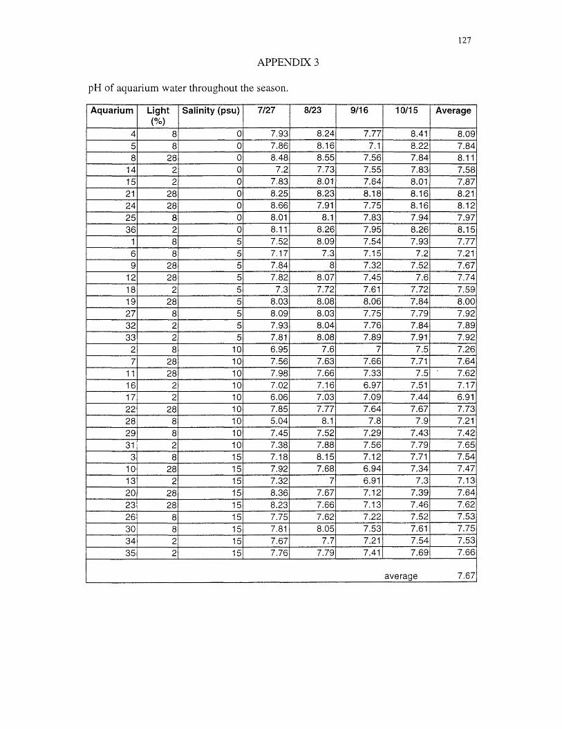
APPENDIX 3

pH of aquarium water throughout the season.

127

Aquarium Light(%)

Salinity (psu) 7/27 8/23 9/16 10/15 Average

4 8 0 7.93 8.24 7.77 8.41 8.095 8 0 7.86 8.16 7.1 8.22 7.848 28 0 8.48 8.55 7.56 7.84 8.11

14 2 0 7.2 7.73 7.55 7.83 7.5815 2 0 7.83 8.01 7.64 8.01 7.8721 28 0 8.25 8.23 8.18 8.16 8.2124 28 0 8.66 7.91 7.75 8.16 8.1225 8 0 8.01 8.1 7.83 7.94 7.9736 2 0 8.11 8.26 7.95 8.26 8.15

1 8 5 7.52 8.09 7.54 7.93 7.776 8 5 7.17 7.3 7.15 7.2 7.219 28 5 7.84 8 7.32 7.52 7.67

12 28 5 7.82 8.07 7.45 7.6 7.7418 2 5 7.3 7.72 7.61 7.72 7.5919 28 5 8.03 8.08 8.06 7.84 8.0027 8 5 8.09 8.03 7.75 7.79 7.9232 2 5 7.93 8.04 7.76 7.84 7.8933 2 5 7.81 8.08 7.89 7.91 7.92

2 8 10 6.95 7.6 7 7.5 7.267 28 10 7.56 7.63 7.66 7.71 7.64

11 28 10 7.98 7.66 7.33 7.5 7.6216 2 10 7.02 7.16 6.97 7.51 7.1717 2 10 6.06 7.03 7.09 7.44 6.9122 28 10 7.85 7.77 7.64 7.67 7.7328 8 10 5.04 8.1 7.8 7.9 7.2129 8 10 7.45 7.52 7.29 7.43 7.4231 2 10 7.38 7.88 7.56 7.79 7.65

3 8 15 7.18 8.15 7.12 7.71 7.5410 28 15 7.92 7.68 6.94 7.34 7.4713 2 15 7.32 7 6.91 7.3 7.1320 28 15 8.36 7.67 7.12 7.39 7.6423 28 15 8.23 7.66 7.13 7.46 7.6226 8 15 7.75 7.62 7.22 7.52 7.5330 8 15 7.81 8.05 7.53 7.61 7.7534 2 15 7.67 7.7 7.21 7.54 7.5335 2 15 7.76 7.79 7.41 7.69 7.66

average 7.67

APPENDIX 4

128

Flowering structures observed.

Date Light (%) Salinity (psu) Aquarium # Flowers8/2 28 0 24 3

8 5 27 228 5 19 1

8/16 28 0 24 48 5 27 5

28 5 9 18/29 8 0 5 1

28 0 8 128 5 9 128 0 24 2

8 5 27 49/14 8 0 5 1

28 0 8 29/27 28 0 8 1

129

APPENDIX 5

Sample size for quantum yield and ETRmax measurements. n=3 unless otherwise noted. n<3 due to leaf senescence.

Quantum Yield

Salinity Light (psu) (%)

6/22 7/6 7/22 8/2 8/17 9/1 9/13 9/29

0 28 8 2

2

2 2 25 28

8 2 2

10 28 8 2

2 2 1

15 28 8 2

2 2 2 2 2 2 12 2 1 0

2 2 2 1 0

ETR, August 20

n=2 for the following:

Salinity(psu)

Light(%)

0 285 810 2815 28

82

ETR, September 12

n=2 for the following:

Salinity Light(psu) (%)5 815 28

8

n=l for the following:

Salinity Light(psu) (%)15 2

13 0

LITERATURE CITED

Adair, S.E., J.L. Moore, and C.P. Onuf. 1994. Distribution and Status of submerged vegetation in estuaries of the upper Texas coast. Wetlands 14(2): 110-121.

Adams, J. B. and G. C. Bate. 1994. The ecological implications of tolerance to salinity by Ruppia cirrhosa (Petagna) Grande and Zostera capensis Setchell. Botanica Marina 37(5): 449-456.

Asch, F. M. Dingkuhn, and K. Dorffling. 2000. Salinity increases CO2 assimilation but reduces growth in field-grown, irrigated rice. Plant and Soil 218(1-2): 1-10.

Barko, J.W. and R.M. Smart. 1981. Comparative influences of light and temperature on the growth and metabolism of selected submersed freshwater macrophytes. Ecological Monographs 51: 219-235.

Barko, J.W., D.G. Hardin, and M.S. Matthews. 1982. Growth and morphology ofsubmersed freshwater macrophytes in relation to light and temperature. Canadian Journal o f Botany 60: 877-887.

Barko, J.W., R.M. Smart, and D. G. McFarland. 1991. Interactive effects ofenvironmental conditions on the growth of submersed aquatic macrophytes. Journal o f Freshwater Ecology 6(2): 199-207.

Batiuk, R.A., R.J. Orth, K.A. Moore, W.C. Dennison, J.C. Stevenson, L. Staver, V. Carter, N. Rybicki, R.E. Hickman, S. Kollar, S. Bieber, P. Heasly, and P. Bergstrom. 1992. Chesapeake Bay submerged aquatic vegetation habitat requirements and restoration targets: A technical synthesis. CBP/TRS 83/92. U.S. Environmental Protection Agency, Chesapeake Bay Program, Annapolis, Maryland.

Bayley, S., V.D. Stotts, P.F. Springer, and J. Steenis. 1978. Changes in submergedaquatic macrophyte populations at the head of the Chesapeake Bay, 1958-1974. Estuaries 1: 171-182.

Beer, S., B. Vilenkin, A. Weil, M. Veste, L. Susel, and A. Eshel. 1998. Measuring photosynthetic rates in seagrasses by pulse amplitude modulated (PAM) fluorometry. Marine Ecology Progress Series 174: 293-300.

131

Beer, S. and M. Bjork. 2000. Measuring rates of photosynthesis of two tropicalseagrasses by pulse amplitude modulated (PAM) fluorometry. Aquatic Botany 66: 69-76.

Beer, S., C. Larsson, O. Poryan, and L. Axelsson. 2000. Photosynthetic rates of Ulva (Chlorophyta) measured by pulse amplitude modulated (PAM) fluorometry. European Journal o f Phycology 35( 1): 69-74.

Beer, S., M. Ilan, A. Eshel, A. Weil, and I. Brickner. 1998a. Use of pulse amplitudemodulated (PAM) fluorometry for in situ measurements of photosynthesis in two Red Sea faviid corals. Marine Biology 131(4): 607-612.

Beer, S., B. Vilenkin, A. Weil, M. Veste, L. Susel, and A. Eshel. 1998b. Measuring photosynthetic rates in seagrasses by pulse amplitude modulated (PAM) fluorometry. Marine Ecology Progress Series 174: 293-300.

Beer. S. and M. Ilan. 1998. In situ measurements of photosynthetic irradiance responses of two Red Sea sponges growing under dim light conditions. Marine Biology 131(4): 613-617.

Bjork, M., J.N. Uku, A Weil and S. Beer. 1999. Photosynthetic tolerances to dessication of tropical intertidal seagrasses. Marine Ecology Progress Series 191: 121-126.

Bjorkman, O. and B. Demmig. 1987. Photon yield of 02-evolution and chlorophyll fluorescence characteristics at 77 K among vascular plants of diverse origins. Planta 170: 489-504.

Blanch, S.J., G.G. Ganf, and K.F. Walker. 1998. Growth and recruitment in Vallisneria americana as related to average irradiance in the water column. Aquatic Botany 61: 181-205.

Bloom, A.J., F.S. Chapin, IE, and H.A. Mooney. 1985. Resource limitation in plants— an economic analogy. Annual Review o f Ecology and Systematics 16: 363-392.

Brenchley, J. L. and R. J. Probert. 1998. Seed germination responses to someenvironmental factors in the seagrass Zostera capricorni from eastern Australia. Aquatic Botany 62(3): 177-188.

Carter, V. and N.B. Rybicki. 1985. Effects of grazers and light penetration on the survival of transplants of Vallisneria americana Michx in the tidal Potomac River, Maryland. Aquatic Botany 23(3): 197-213.

Carter, V. and N.B. Rybicki. 1986. Resurgence of submersed aquatic macrophytes in the tidal Potomac River, Maryland, Virginia, and the District of Columbia. Estuaries 9(4B): 368-375.

132

Carter, V., N.B. Rybicki, and M. Turtora. 1996. Effect of increasing photon irradiance on the growth of Vallisneria americana in the tidal Potomac River. Aquatic Botany 54(4): 337-345.

Carter, V., N.B. Rybicki, J.M. Landwehr, and M. Naylor. 2000. Light requirements for SAV survival and growth, in Chesapeake Bay SAV water quality and habitat- based requirements and restoration targets: A second technical synthesis. U.S. EPA. Chesapeake Bay Program.

Champ, M.A., G.A. Gould III, W.E. Bozzo, S.G. Ackleson, and K.C. Vierra. 1980.Characterization of light extinction and attenuation in Chesapeake Bay, August 1977. In: Kennedy, V.S. (Ed.), Estuarine Perspectives, Academic Press, New York, pp. 263-277.

Chapin, F.S. Ill, A.J. Bloom, C.B. Field, and R.H. Waring. 1987. Plant responses tomultiple environmental factors: Physiological ecology provides tools for studying how interacting environmental resources control plant growth. BioScience 37(1): 49-57.

Conacher, C. A., I. R. Poiner, J. Bulter, S. Pun, and D. J. Tree. 1994. Germination, storage, and viability testing of seeds of Zostera capricorni Aschers from a tropical bay in Australia. Aquatic Botany 62(3): 177-188.

Dennison, W.C. 1990. Chlorophyll content. In Seagrass Research Methods. R.C. Phillips and C.P. McRoy (eds.). Unesco, Paris.

Dennison, W.C., R.J. Orth, K.A. Moore, J.C. Stevenson, V. Carter, S. Kollar, P.W. Bergstrom, and R.A. Batiuk. 1993. Assessing water quality with submersed aquatic vegetation: Habitat requirements as barometers of Chesapeake Bay health. BioScience 43(2): 86-94.

Dionisio-Sese, M.L. and S. Tobita. 2000. Effects of salinity on sodium content andphotosynthetic responses of rice seedlings differing in salt tolerance. Journal o f Plant Physiology 157(1): 54-58.

Dring, M.J. 1986. The Biology o f Marine Plants. Edward Arnold, London.

Dunton, K.H. 1996. Photosynthetic production and biomass of the subtropical seagrass Halodule wrightii along an estuarine gradient. Estuaries 19(2): 436-447.

Genty, B. J.M. Briantais, and N.R. Baker. 1989. The relationship between quantum yield of photosynthetic electron transport and quenching of chlorophyll fluorescence. Biochimica et Biophysica Acta 990: 87-92.

133

Giesy, J.P. Jr. and E.P. Odum. 1980. Microcosmology: introductory comments. In: Giesy J.P. (ed) Microcosms in ecological research. Technical Information Center, U.S. Department of Energy, Symposium Series No. 52, pp. 1-13.

Goodman, J.L., K.A. Moore, and W.C. Dennison. 1995. Photosynthetic responses of eelgrass {Zostera marina L.) to light and sediment sulfide in a shallow barrier island lagoon. Aquatic Botany 50: 37-47.

Grise, D., J.E. Titus, and D.J. Wagner. 1986. Environmental pH influences growth and tissue chemistry of the submersed macrophyte Vallisneria americana. Canadian Journal of Botany 64: 306-310.

Hale, M.G. and D.M. Orcutt. 1987. The Physiology o f Plants Under Stress. John Wiley and Sons, Inc., New York.

Haller, W.T., D.L. Sutton, and W. C. Barlowe. 1974. Effects of salinity on growth of several aquatic macrophytes. Ecology 55: 891-894.

Haller, W.T. and D.L. Sutton. 1975. Community structure and competition between Hydrilla and Vallisneria. Hyacinth Control Journal 13: 48-50.

Haramis, G.M. and V. Carter. 1983. Distribution of submersed aquatic macrophytes in the tidal Potomac River. Aquatic Botany 15: 65-79.

Havaux, M. 1992. Stress tolerance of photosystem II in vivo. Plant Physiology 100: 424- 432.

Hootsmans M.J.M. and J.E. Vermaat. 1991. Macrophytes, a key to understandingchanges caused by eutrophication in shallow freshwater ecosystems. International Institute for Hydraulic and Environmental Engineering Report Series 21, The Netherlands.

Hopkinson, C.S. Jr., A.E. Giblin, J. Tucker, and R.H. Garritt. 1999. Benthic metabolism and nutrient cycling along an estuarine salinity gradient. Estuaries 22(4): 863- 881.

Howe, H.F. and J. Smallwood. 1982. Ecology of seed dispersal. Annual Review o f Ecology and Systematics 13: 201-228.

Inglis, G.J. 2000. Variation in the recruitment behavior of seagrass seeds: implications for population dynamics and resource management. Pacific Conservation Biology 5: 251-259.

Kamermans, P., M.A. Hemminga, and D.J. Jong. 1999. Significance of salinity and silicon levels for growth of a formerly estuarine eelgrass (Zostera marina)

134

population (Lake Grevelingen, The Netherlands). Marine Biology 133(3): 527-539.

Kaul, R.B. 1978. Morphology of germination and establishment of aquatic seedlings in Alismataceae and Hydrocharitaceae. Aquatic Botany 5: 139-147.

Kemp, W. M., R. R. Twilley, J. C. Stevenson, W. R. Boynton, and J. C. Means. 1983.The decline of submerged vascular plants in upper Chesapeake Bay: Summary of results concerning possible causes. Marine Technology Society Journal 17(2): 78- 89.

Kerr, E. A. and S. Strother. 1985. Effects of irradiance, temperature and salinity on photosynthesis of Zostera muelleri. Aquatic Botany 23(2): 177-184.

Khan, M. A. and I. A. Ungar. 1999. Effect of salinity on seed germination of Triglochin maritima under various temperature regimes. Great Basin Naturalist 58(2): 144- 150.

Kimber, A., C. E. Korschgen, and A. G. Van der Valk. 1995. The distribution of Vallisneria americana seeds and seedling light requirements in the Upper Mississippi River. Canadian Journal o f Botany 73(12): 1966-1973.

Kirk, J.T.O. 1994. Light and photosynthesis in aquatic ecosystems. Cambridge University Press, Cambridge. 509 pp.

Koroleva, O.Y., W. Bruggemann, and G. H. Krause. 1994. Photoinhibition, xanthophyll cycle and in vivo chlorophyll fluorescence quenching of chilling-tolerant Oxyria digyna and chilling sensitive Zea mays. Physiologia Plantarum 92: 577-584.

Korschgen, C. E. and W. L. Green. 1988. American wild celery (Vallisneria americana): Ecological considertions for restoration. Technical Report Series U. S. Fish and Wildlife Service, 31 pp.

Korschgen, C. E., W. L. Green, and K. P. Kenow. 1997. Effects of irradiance on growth and winter bud production by Vallisneria americana and consequences to its abundance and distribution. Aquatic Botany 58(1): 1-9.

Kraemer, G. P., R. H. Chamberlain, P. H. Doering, A. D. Steinman, and M. D. Hanisak. 1999. Physiological responses of transplants of the freshwater angiosperm Vallisneria americana along a salinity gradient in the Caloosahatchee Estuary (southwestern Florida). Estuaries 22(1): 138-148.

Kromkamp, J. C. Barranguet, and J. Peene. 1998. Determination of microphytobenthos PSD quantum efficiency and photosynthetic activity by means of variable chlorophyll fluorescence. Marine Ecology Progress Series 162: 45-55.

135

Lazar, A.C. and C.J. Dawes. 1991. A seasonal study of the seagrass Ruppia maritima L. in Tampa Bay, Florida. Organic constitutents and tolerances to salinity and temperature. Botanica marina 34: 265-269.

Longstaff, B.J., N.R. Loneragan, M.J. O’Donohue, and W.C. Dennison. 1999. Effects of light deprivation on the survival and recovery of the seagrass Halophila ovalis (R.Br.) Hook. Journal o f Experimental Marine Biology and Ecology 234(1): 1-27.

Lowden, R.M. 1982. An approach to the taxonomy of Vallisneria L. (Hydrocharitaceae). Aquatic Botany 13: 269-298.

Masini, R.J., J.L. Cary, C.J. Simpson, and A.J. McComb. 1995. Effects of light andtemperature on the photosynthesis of temperate meadow-forming seagrasses in Western Australia. Aquatic Botany 49: 239-254.

Masini, R.J. and C.R. Manning. 1997. The photosynthetic responses to irradiance and temperature of four meadow-forming seagrasses. Aquatic Botany 58: 21-36.

Maxwell, K. and G.N. Johnson. 2000. Chlorophyll fluorescence - a practical guide. Journal o f Experimental Botany 51(345): 659-668.

Meyer, B.S., F.H. Bell, L.C. Thompson, and E.I. Clay. 1943. Effect of depth ofimmersion on apparent photosynthesis in submersed vascular aquatics. Ecology 24: 393-399.

Moore, K.A., R.J. Orth, and J.F. Nowak. 1993. Environmental regulation of seedgermination in Zostera marina L. (eelgrass) in Chesapeake Bay: Effects of light, oxygen and sediment burial. Aquatic Botany 45(1): 79-91.

Moore, K.A., H.A. Neckles, and R.J. Orth. 1996. Zostera marina (eelgrass) growth and survival along a gradient of nutrients and turbidity in the lower Chesapeake Bay. Marine Ecology Progress Series 142: 247-259.

Moore, K.A., R.L. Wetzel, and R.J. Orth. 1997. Seasonal pulses of turbidity and their relations to eelgrass (Zostera marina L.) survival in an estuary. Journal o f Experimental Marine Biology and Ecology 215: 115-134.

Moore, K.A., D.J. Wilcox, and R.J. Orth. 2000a. Analysis of abundance of submersed aquatic vegetation communities in the Chesapeake Bay. Estuaries 23: 115-127.

Moore, K.A., R.J. Orth, and J. Fishman. 2000b. Restoration of submerged aquaticvegetation (SAV) in the tidal freshwater James River: 1999 pilot study. Special Report No. 365 in Applied Marine Science and Ocean Engineering.

136

Morlock, S. D. Taylor, A. Giblin, C. Hopkinson, and J. Tucker. 1997. Effect of salinity on the fate of inorganic nitrogen in sediments of the Parker River Estuary, Massachusetts. Biological Bulletin 193: 290-292.

Orth, R.J. and K.A. Moore. 1983. Chesapeake Bay: An unprecedented decline in submerged aquatic vegetation. Science 222: 51-53.

Orth, R.J. and K.A. Moore. 1984. Distribution and abundance of submerged aquatic vegetation in Chesapeake Bay: A historical perspective. Estuaries 7(4B): 531 -540.

Orth, R.J., M. Luckenbach, and K.A. Moore. 1994. Seed dispersal in a marinemacrophyte: implications for colonization and restoration. Ecology 75(7): 1927- 1939.

Orth, R.J., R.A. Batiuk, and J.F. Nowak. 1994. Trends in the Distribution, Abundance,and Habitat Quality o f Submerged Aquatic Vegetation in Chesapeake Bay and its Tidal Tributaries: J971-199L Chesapeake Bay Program, Annapolis, MD. CBP/TRS 137/95. EPA 903-R-95-009. 216 pp.

Orth, R.J., J.F. Nowak, D.J. Wilcox, J.F. Whiting, and L.S. Nagey. 1999. Distribution of submerged aquatic vegetation in the Chesapeake Bay and Coastal Bays - 1998. Virginia Institute of Marine Science. Gloucester Point, VA. 370 pp.

Parsons, T.R., Y. Maita, and C.M. Lalli. 1984. A Manual of Chemcial and Biological Methods for Seawater Analysis, Pergamon Press, New York, 173 pp.

Perez, M. and J. Romero. 1992. Photosynthetic response to light and temperature of the seagrass Cymodocea nodosa and the prediction of its seasonality. Aquatic Botany 43:51-62.

Philbrick, C.T. and D.H. Les. 1996. Evolution of aquatic angiosperm reproductivesystems: What is the balance between sexual and asexual reproduction in aquatic angiosperms? Bioscience 46(11).

Poljakoff-Mayber, A., G. F. Somers, E. Werker, and J. L. Gallagher. 1994. Seeds of Kosteletzkya virginica (Malvaceae): Their structure, germination, and salt tolerance. 2. Germination and salt tolerance. American Journal o f Botany 81(1): 54-59.

Prange, J.A. and W.C. Dennison. 2000. Marine Pollution Bulletin 41(7-12): 327-336.

Ralph, P.J. and M.D. Burchett. 1995. Photosynthetic responses of the seagrass Halophila ovalis (R. Br.) Hook. f. to high irradiance stress, using chlorophyll a fluorescence. Aquatic Botany 51: 55-66.

137

Ralph, P.J. 1996. Diurnal photosynthetic patterns of Halophila ovalis (R. Br.) Hook/ Seagrass Biology: Proceedings of an International Workshop. Rottnest Island, Western Australia, 25-29 January 1996. 197-202.

Ralph, P.J. and M.D. Burchett. 1998a. Impact of petrochemicals on the photosynthesis of Halophila ovalis using chlorophyll fluorescence. Marine Pollution Bulletin 36(6): 429-436.

Ralph, P.J. and M.D. Burchett. 1998b. Photosynthetic response of Halophila ovalis to heavy metal stress. Environmental Pollution 103: 91-101.

Ralph, P.J., R. Gademann, and W.C. Dennison. 1998. In situ seagrass photosynthesis measured using a submersible, pulse-amplitude modulated fluorometer. Marine Biology 132: 367-373.

Ralph. P.J. 1998a. Photosynthetic response of Halophila ovalis (R. Br.) H o o k ./ toosmotic stress. Journal o f Experimental and Marine Biology and Ecology 227: 203-220.

Ralph, P.J. 1998b. Photosynthetic response of laboratory-cultured Halophila ovalis to thermal stress. Marine Ecology Progress Series 171: 123-130.

Ralph, P.J. 1999a. Herbicide toxicity of Halophila ovalis assessed by chlorophyll a fluorescence. Aquatic Botany 1349: 1-12.

Ralph, P.J. 1999b. Light-induced photoinhibitory stress responses of laboratory-cultured Halophila ovalis. Botanica Marina 42: 11-22.

Ralph, P.J. 1999c. Photosynthetic response of Halophila ovalis (R. Br.) Hook./, to combined environmental stress. Aquatic Botany 1329: 1-14.

Romero-Aranda, R., T. Soria, and J. Cuartero. 2001. Tomato plant-water uptake and plant-water relationships under saline growth conditions. Plant Science 160(2): 265-272.

Rout, N.P. and B.P. Shaw. 2001. Salt tolerance in aquatic macrophytes: Possible involvement of the antioxidative enzymes. Plant Science 160(3): 415-423.

Rybicki, N.B. and V. Carter. 1986. Effect of sediment depth and sediment type on thesurvival of Vallisneria americana Michx grown from tubers. Aquatic Botany 24: 233-240.

Sand-Jensen, K. and J. Borum. 1983. Regulation of growth of eelgrass (.Zostera marina L.) in Danish coastal waters. Marine Technology Society Journal 17(2): 15-21.

138

Schreiber, U., W. Bilger and C. Neubauer. 1994. Chlorophyll fluorescence as anonintrusive indicator for rapid assessment of in vivo photosynthesis. Ecological Studies: Analysis and Synthesis 100: 49-70.

Sculthorpe, C.D. 1967. The biology of aquatic vascular plants. St. Martin’s Press, New York. 610 pp.

Spencer, D.F., G.G. Ksander, J.D. Madsen and C.S. Owens. 2000. Emergence of vegetative propagules of Potamogeton nodosus, Potamogeton pectinatus, Vallisneria americana, and Hydrilla verticillata based on accumulated degree- days. Aquatic Botany 67: 237-249.

Staver, L.W. 1986. Competitive interactions of submersed aquatic vegetation under varying nutrient and salinity conditions. Thesis, University of Maryland.

Steindler, L, S. Beer, A. Peretzman-Shemer, C. Nyberg, and M. Dan. 2001.Photoadaptation of zooxanthellae in the sponge Cliona vastifica from the Red Sea, as measured in situ. Marine Biology 138(3): 511-515.

Stevenson, J.C., C.B. Piper, and N. Confer. 1979. The decline of submerged aquaticplants in the Chesapeake Bay. U.S. Fish and Wildlife Service, FWS/OBS-79/24.12 pp.

Stevenson, J.C., L.W. Staver, and K.W. Staver. 1993. Water quality associated withsurvival of submersed aquatic vegetation along an estuarine gradient. Estuaries 16(2): 346-361.

Stross, R.G. 1979. Density and boundary regulations of the Nitella meadow in Lake George, New York. Aquatic Botany 6: 285-300.

Titus, J.E. and M.S. Adams. 1979. Coexistence and the comparative light relations of the submersed macrophytes Myriophyllum spicatum L. and Vallisneria americana Michx. Oecologia 40: 273-286.

Titus, J.E. and M.D. Stephens. 1983. Neighbor influences and seasonal growth patterns for Vallisneria americana Michx. Oecologia 56: 23-29.

Titus, J.E. and W.H. Stone. 1982. Photosynthetic response of two submersedmacrophytes to dissolved inorganic carbon concentration and pFL Limnology and Oceanography 27(1): 151-160.

Twilley, R. R. and J. W. Barko. 1990. The growth of submersed macrophytes under experimental salinity and light conditions. Estuaries 13(3): 311-321.

139

U.S. Environmental Protection Agency. 1979. Manual of methods for chemical analysis of water and wastes. EPA-600-4-79-020. Environmental Monitoring and Support Laboratory. Cincinnati, OH, 460 pp.

Van Dijk, G.M. 1991. Light climate and its impacts on Potamogeton pectinatus L. in a shallow eutrophic lake.

Walker, D. I. and A. J. McComb. 1990. Salinity response of the seagrass Amphibolis antarctica (Labill.) Sonder et Aschers.: An experimental validation of field results. Aquatic Botany 36(4): 359-366.

Walz, Heinz. 1998. Underwater Fluorometer: Diving-PAM. Submersible Photosynthesis Yield Analyzer. Handbook of Operation. Germany.

Wang, D, M.C. Shannon, and C.M. Grieve. 2001. Salinity reduces radiation absorption and use efficiency in soybean. Field Crops Research 69(3): 267-277.

White, A.J. and C. Critchley. 1999. Rapid light curves: A new fluorescence method to assess the state of the photosynthetic apparatus. Photosynthesis Research 59: 63- 72.

140

VITA

GAIL T. FRENCH

Born in Boston, MA, 31 March 1974. Graduated from Belmont High School in 1992. Earned B.A. in Biology from Williams College in 1996. Entered masters program in College of William and Mary, School of Marine Science in 1999.

effects of light and salinity stress on vallisneria

Documents