effects of habitat loss and fragmentation on population...

Contributed Papers

Effects of Habitat Loss and Fragmentation onPopulation DynamicsTHORSTEN WIEGAND∗§, ELOY REVILLA∗†, AND KIRK A. MOLONEY‡∗Department of Ecological Modelling, UFZ-Centre for Environmental Research, PF 500136, D-04301 Leipzig, Germany‡Department of Ecology, Evolution and Organismal Biology, 143 Bessey Hall, Iowa State University, Ames, Iowa 50011, U.S.A.

Abstract: We used a spatially explicit population model that was generalized to produce nine ecologicalprofiles of long-lived species with stable home ranges and natal dispersal to investigate the effects of habitatloss and fragmentation on population dynamics. We simulated population dynamics in landscapes composedof three habitat types (good-quality habitat ranging from 10–25%, poor-quality habitat ranging from 10–70%, and matrix). Landscape structures varied from highly fragmented to completely contiguous. The specificaims of our model were (1) to investigate under which biological circumstances the traditional approach ofusing two types only (habitat and matrix) failed and assess the potential impact of restoring matrix to poor-quality habitat, (2) to investigate how much of the variation in population size was explained by landscapecomposition alone and which key attributes of landscape structure can serve as predictors of populationresponse, and (3) to estimate the maximum fragmentation effects expressed in equivalent pure loss of good-quality habitat. Poor-quality habitat mattered most in situations when it was generally not considered (i.e.,for metapopulations or spatially structured populations when it provides dispersal habitat). Population sizeincreased up to 3 times after restoring matrix to poor-quality habitat. Overall, habitat amount accountedfor 68% of the variation in population size, whereas ecological profile and fragmentation accounted forapproximately 13% each. The maximal effect of (good-quality) habitat fragmentation was equivalent to apure loss of up to 15% of good-quality habitat, and the maximal loss of individuals resulting from maximalfragmentation reached 80%. Abundant dispersal habitat and sufficiently large dispersal potential, however,resulted in functionally connected landscapes, and maximal fragmentation had no effect at all. Our findingssuggest that predicting fragmentation effects requires a good understanding of the biology and habitat useof the species in question and that the uniqueness of species and the landscapes in which they live confoundsimple analysis.

Key Words: ecological profiles, individual-based spatially explicit population model, landscape metrics, land-scape structure, matrix heterogeneity, metapopulation, source-sink

Efectos de la Perdida y Fragmentacion del Habitat sobre la Dinamica Poblacional

Resumen: Para investigar los efectos de la perdida y fragmentacion del habitat sobre la dinamica poblacionalutilizamos un modelo poblacional espacialmente explıcito generalizado para nueve perfiles ecologicos deespecies longevas con rangos de hogar estables y dispersion natal. Simulamos la dinamica poblacional enpaisajes compuestos por tres tipos de habitat (habitat de buena calidad de 10-25%, habitat de pobre calidadde 10-70% y matriz). Las estructura del paisaje vario desde altamente fragmentado a completamente contiguo.Las metas especıficas de nuestro modelo fueron (1) investigar las circunstancias biologicas en las que fallael metodo tradicional de usar solo dos tipos (habitat, matriz) y evaluar el impacto potencial de restaurar lamatriz a habitat de pobre calidad, (2) investigar cuanta variacion en el tamano de la poblacion se explicaba

§email [email protected]†Current address: Department of Applied Biology, Estacion Biologica de Donana, Ave Maria Luisa s/n, Pabellon del Peru, 41013 Sevilla, Spain.Paper submitted May 12, 2003; revised manuscript accepted May 7, 2004.

108

Conservation Biology, Pages 108–121Volume 19, No. 1, February 2005

Wiegand et al. Habitat Loss and Fragmentation 109

solo por la composicion del paisaje y cuales atributos clave de la estructura del paisaje pueden servir comopredoctores de la respuesta poblacional y (3) estimar los maximos efectos de la fragmentacion expresados en laperdida equivalente de habitat de buena calidad. El habitat de pobre calidad fue mas importante en situacionesen que generalmente no era considerado (i.e. cuando proporciona habitat de dispersion para metapoblacioneso poblaciones espacialmente estructuradas). El tamano poblacional incremento hasta tres veces despues derestaurar la matriz a habitat de pobre calidad. En total, la cantidad de habitat explico 68% de la variacion enel tamano de la poblacion, mientras que el perfil ecologico y la fragmentacion explicaron aproximadamente13% cada uno. El maximo efecto de fragmentacion de habitat (de buena calidad) fue equivalente a unaperdida pura de hasta 15% habitat de buena calidad, y la maxima perdida de individuos debido a la maximafragmentacion alcanzo 80%. Sin embargo, abundante habitat de dispersion y un potencial de dispersionsuficientemente grande resultaron en paisajes funcionalmente conectados, donde la maxima fragmentacionno tuvo efecto alguno. Nuestros hallazgos sugieren que la prediccion de efectos de la fragmentacion requierede un buen entendimiento de la biologıa y uso de habitat de la especie en cuestion y que la unicidad de lasespecies y de los paisajes en que viven confunden los analisis simples.

Palabras Clave: estructura del paisaje, fuente-vertedero, heterogeneidad de la matriz, metapoblacion, metricasde paisaje, modelo poblacional espacialmente explıcito basado en individuo, perfiles ecologicos

Introduction

Fragmentation and loss of habitat, which are major threatsto the viability of endangered species, have become an im-portant subject of research in ecology (Soule 1986; For-man 1996). Reduction of the total amount of suitable habi-tat results in heterogeneous landscapes composed of iso-lated patches of suitable habitat of varying quality embed-ded in a hostile matrix (Noss & Csuti 1997). This processusually results in both pure habitat loss and fragmentationeffects (Andren 1994). Here we refer to pure habitat lossas changes in landscape composition that cause a pro-portional loss of individuals from the landscape and tofragmentation effects as additional effects resulting fromthe configuration of habitat (i.e., brought about throughreduction in habitat patch size and isolation of habitatpatches, sensu Andren 1994). Many studies have con-vincingly demonstrated that the effects of this reductionon resident populations can be significant (Andren 1994;Fahrig & Merriam 1994; Noss & Csuti 1997; Bender et al.1998).

Most contemporary researchers studying the impor-tance of habitat loss versus fragmentation have used sim-ple models for hypothetical species (e.g., Andren 1996;Bascompte & Sole 1996; Fahrig 1997; Boswell et al. 1998;Hill & Caswell 1999; Hiebeler 2000; Flather & Bevers2002). These models generally contain strong, implicitassumptions (e.g., random-walk dispersal and only twohabitat types, matrix and habitat), and because of theirsimplicity they do not include important processes thatmay affect a real population in fragmented landscapes.The results of these studies are characterized by a consid-erable degree of ambiguity. Some argue that habitat lossfar outweighs the effects of habitat fragmentation (e.g.,Fahrig 1997, 2001), whereas others argue the opposite(e.g., Hiebeler 2000).

The varying results regarding the relative importanceof habitat composition and configuration are likely to berelated to the variety of assumptions in the different mod-els (Flather & Bevers 2002). Additionally, critical speciesattributes have not been varied systematically and there-fore the results have not been put into perspective.

We argue that further progress in investigating the im-pact of habitat loss and fragmentation on population dy-namics cannot be made without providing models withmore biological realism—thus making more of the modelassumptions explicit—and without putting the results ina broader perspective of varying species attributes. Thiscan be done best with spatially explicit, individual-basedmodels (Dunning et al. 1995; Gustafson & Gardner 1996;Wiegand et al. 1999) that allow the inclusion of behav-ioral rules that describe the response of individuals tothe landscape and link the individual’s use of space (dis-persal and habitat selection) directly to population andmetapopulation phenomena.

To systematically investigate the relative effects of habi-tat loss and fragmentation on population dynamics, wesimulated population dynamics in a range of landscapesthat differ in composition and configuration, spanningthe state space associated with habitat configuration fromhighly fragmented to completely contiguous landscapes.We focused on three specific questions. First, we usedthree types of habitat (good-quality habitat, poor-qualityhabitat, and matrix) and asked under which biological cir-cumstances poor-quality habitat matters. This questionchallenges the traditional approach of using only twohabitat types (habitat and matrix) but is also important formanagement in assessing the potential impact of restor-ing matrix to poor-quality habitat. Second, we asked howmuch of the variation in population size is explained bylandscape composition alone and which key attributes oflandscape structure can serve as predictors of population

Conservation BiologyVolume 19, No. 1, February 2005

110 Habitat Loss and Fragmentation Wiegand et al.

response. Finally, we estimated the maximum fragmenta-tion effects expressed in terms of equivalent pure (good-quality) habitat loss.

Methods

We used a previously developed spatially explicit popula-tion model (Wiegand et al. 1999), shaped in accordanceto the biology of European brown bears (Ursus arctos).Because the answers to our questions critically dependon the underlying biology of the model species (e.g., dis-persal abilities and habitat requirements), we generalizedthe critical components of the population model withrespect to habitat fragmentation and created nine ecolog-ical profiles (Vos et al. 2001) that represent a spectrumof long-lived species with stable home ranges and nataldispersal.

Population Model

The model is an individual-based and spatially explicitpopulation model that simulates the demographics, dis-persal, and selection of home ranges of female bears. Themodel rules are described in the Appendix (for more de-tails see Wiegand et al. 1999). Here we briefly describehow landscape structure affects population dynamics.

Individual landscapes consisted of three types of habi-tat: good-quality habitat (G), poor-quality habitat (P), andhostile matrix (M), and were composed of a 50 × 50 gridof cells. Demographic parameters were adjusted to pro-duce an overall rate of population increase of λ > 1.03(λ < 0.99) for landscapes consisting completely of good-(or poor-) quality habitat (for details see Wiegand et al.1999, Fig. 6), and matrix was uninhabitable. A home rangeof maximum size occupied a 3 × 3 area of cells, butsmaller home ranges could occur in highly suitable habitatareas (see Appendix). We included density dependenceby reducing the habitat suitability of a cell if it was sharedby resident females (see Appendix).

Habitat suitability linked the demographic processesto the landscape. A dispersing female (an independentfemale without its own home range) established a homerange if the total habitat suitability of the 3 × 3 cell areasurrounding its present location exceeded a threshold(the minimal resource requirements Qmin). Survival of res-ident females and dependent cubs was higher if the meanhabitat suitability of the home range was higher. During 1year, dispersal consisted of a directed random walk of upto Smax steps through the landscape. The path taken andthe risk of mortality depended on habitat suitability alongthe dispersal path (see Appendix). Movement continueduntil the dispersing female established a home range, untilSmax dispersal steps were taken, or until she died. Surviv-ing females that did not establish a home range during

a model year continued dispersing in the following year.Once a female located a suitable home range, she stayedin that location until she died. Only females occupying ahome range could reproduce.

The Ecological Profiles

Dispersal and establishment of home ranges are the keyprocesses that link demography to the landscape. There-fore, we created an array of ecological profiles that dif-fered in the maximal number of dispersal steps (Smax)taken during 1 year and in the habitat suitability thresh-old (Qmin) for establishment of a home range. We se-lected three values for Smax that corresponded to low,intermediate, and high dispersal abilities (Smax = 4, 16,and 64, respectively). As with Smax, we used three val-ues for the resource requirement parameter (Qmin = 24,32, and 40). For low (Qmin = 24) and moderate (Qmin

= 32) resource requirements, home ranges could be en-tirely composed of poor-quality habitat, whereas a homerange with high resource requirements (Qmin = 40) hadto contain at least two good-quality habitat cells (see Ap-pendix). The range of resource requirements used in dif-ferent model runs corresponded to different strategies forhandling the trade-off between the high risk of mortalityin home ranges of low suitability home ranges and thehigh risk of mortality when dispersing longer distancesin search of a better quality home range.

The Landscape Model

Landscape composition was determined through a set ofparameters ( fG, fP, and fM) that represented the propor-tion of cells of the three habitat types (G, P, and M) in thelandscape. Wiegand et al. (1999) investigated the corre-lation between key variables of population dynamics andtwo fragmentation measures for 20 largely different land-scape types. Because their results were independent ofthe specific landscape type used, we used five “represen-tative” landscape types here (Fig. 1). The landscape typeswe used ranged from a type that was randomly structuredin terms of the scale of individual home ranges (landscapetype A, see Wiegand et al. 1999) to a type with one con-tiguous area of good-quality habitat (landscape type E).For each landscape type we generated 16 individual land-scape maps (Fig. 2) with different proportions of poor-quality habitat ( fp= 0.1, 0.3, 0.5, and 0.7) and differentproportions of good-quality habitat ( fG = 0.10, 0.15, 0.20,and 0.25). We varied the proportions of good-quality habi-tat only within a relatively small range (�fG = 0.15) be-cause in situations of conservation concern, the amountof good-quality habitat in a landscape is usually quite low,and in such situations loss (or restoration) of good-qualityhabitat may result in levels even below 10% (e.g., McK-elvey et al. 1993; Gaona et al. 1998; Vos et al. 2001).In contrast, we varied the proportion of poor-quality



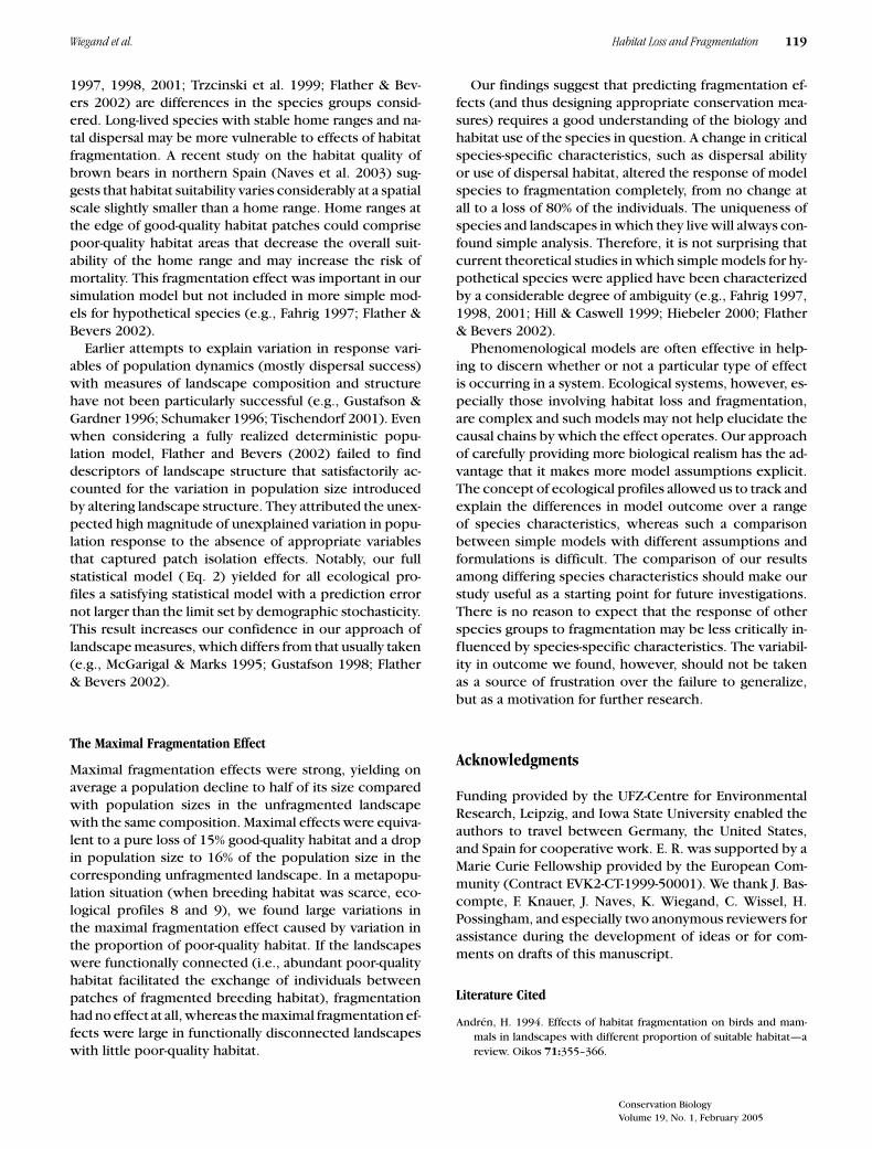
Figure 1. The five landscapes and the values of the fragmentation measures. Top row (A–E): the five landscapetypes that span the state space associated with configuration of good-quality habitat from highly fragmented(landscape type A) to completely contiguous (landscape type E), exemplified for landscapes with 10% good-qualityhabitat (fG = 0.1) and 30% poor-quality habitat (fp = 0.3). Middle row: landscape measure OGN (3) for the 20landscapes of types A to E (OGN [3] is the fraction of cells of poor-quality habitat and matrix at the critical distancercrit = 3 away from cells of good-quality habitat). The OGN (3) does not depend on the proportion of poor-qualityhabitat. Bottom row: the landscape measure OGM (3) for the 20 landscapes of types A to E (OGM [3] gives thefraction of matrix cells at the critical distance rcrit = 3 away from cells of good-quality habitat).

habitat over a wider range (�fG = 0.6), primarily be-cause we sought to assess the role of the third habitattype on population dynamics and the full effect of a po-tential restoration of matrix to poor-quality habitat.

Landscape Measures

Wiegand et al. (1999) introduced two scale-dependentlandscape measures, OGG(r) and OGM(r), which were de-fined as the overall fraction of cells of good-quality habitatand matrix, respectively, at a distance r from cells of good-quality habitat. These investigators found the strongestcorrelations between these measures and key variablesof population dynamics (e.g., average number of sourcehome ranges and mean dispersal distance) at spatial scalesr = 2–4 (Wiegand et al. [1999], Figs. 9, 10, and 12). There-fore, we used only OGG(3) and OGM(3) at the “critical”

scale rcrit = 3. Because OGG(r) = 1 − OGM(r) if no poor-quality habitat exists (i.e., fp = 0) and to give both land-scape measures a consistent interpretation of a fragmen-tation measure, we used here the transformed measureOGN(r) = 1 − OGG(r)—the fraction of poor-quality or ma-trix cells at distance r from cells of good-quality habitat(i.e., N = P or M).

The OGN(rcrit) measures the fragmentation of good-quality habitat at distance rcrit from good-quality habitatcells (Fig. 1, middle row). High values of OGN(rcrit) indi-cate a high probability that other habitat types (i.e., P orM ) can be found at distance rcrit from good-quality habitatcells (i.e., landscape type A). The OGN(rcrit) decreases ifthe landscape type changes under constant compositionfrom the highly fragmented type A to the highly contigu-ous type E (Fig. 1, middle row). It does not, however,reach zero as long as the proportion fG of good-quality



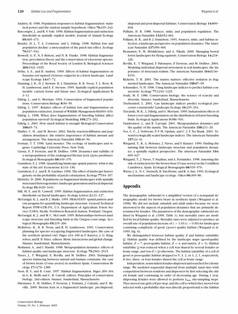
Figure 2. The 16 landscapes withdifferent composition derived fromlandscape type C (this landscapetype shows an intermediate degreeof fragmentation of thegood-quality habitat). Columnsfrom left to right: proportion ofpoor-quality habitat fp = 10%, 30%,50%, and 70%. Rows from top tobottom: proportion of good-qualityhabitat fG = 10%, 15%, 20%, and25%. White cells are good-qualityhabitat, grey cells are poor-qualityhabitat, and black cells are matrixhabitat.

habitat is below 1. The OGN(rcrit) can be interpreted as ameasure of patch-size effects because it was highly corre-lated to the log-log transformation of the mean patch area(rPearson = 0.93, n = 20) and to the number of patches(rPearson = 0.93, n = 20) if we considered only patchesthat could potentially serve as a home range (i.e., patcheswith three or more cells of good-quality habitat).

The OGM(rcrit) measures the fragmentation of the suit-able habitat (i.e., good and poor quality) at distance rcrit

from good-quality habitat cells (Fig. 1, bottom row). Highvalues of OGM(rcrit) indicate a high probability that ma-trix cells are interspersed at scale rcrit from good-qualityhabitat cells (i.e., there are many movement barriers in theproximity of good-quality habitat cells). The OGM(rcrit) de-creases if the proportion fP of poor-quality habitat cells in-creases because the proportion of matrix cells decreases(note that fM = 1 − fG − fP). The OGM(rcrit) also decreasesif the landscape type changes under constant composi-tion from highly fragmented type A to the highly con-tiguous type E (Fig. 1, bottom row) and reaches zero forall landscape types (except type A) if the proportion ofpoor-quality habitat is high.

Model Output for Analyses

As model output for an individual model simulation i, wecalculated the average number of independent females

(nimean), the average number of sink home ranges (ni

sink),and the average number of source home ranges (ni

source),taken for simulation years 100 through 200. Whether ahome range acted as a sink or a source was determinedaccording to its mean habitat suitability (see Wiegand etal. 1999, Fig. 6). We defined source-sink properties basedon the current habitat suitability within a home range,not on a priori habitat types. Additionally, we recordedthe distribution of dispersal distances (i.e., the Euclideandistance between the natal site and the own home range)between simulation years 100 and 200 and used it to cal-culate mean dispersal distance (di

mean), maximum disper-sal distance (di

max), and the distance below which 95% ofthe observed dispersal distances fell within a model run(di

95). Within each landscape we performed 20 replicatesimulations for each ecological profile and calculated theaverage of the variables, which we indicate with capitalN and D (e.g., N mean = 1/20� i=1..20 ni

mean).

Habitat-Matrix Approximation

To assess the maximal effect of poor-quality habitat, wecompared the simulated mean population sizes and themean dispersal distances between corresponding land-scapes with little ( fp = 0.1) and with abundant poor-quality habitat ( fp = 0.7). As a measure of the magnitudeof change resulting from poor-quality habitat, we used



the factor change in mean population size N mean( fp =0.7)/(N mean( fp = 0.1) and the factor change in meandispersal distance Dmean( fp = 0.7)/(Dmean( fp = 0.1).The habitat–matrix approximation holds if the factors ofchange are approximately 1.

Variation in Population Size and the Role of FragmentationMeasures

To address the relative importance of habitat compositionand fragmentation on population size, we used an analy-sis of variance with the four factors: proportion of good-quality habitat, proportion of poor-quality habitat, land-scape type, and ecological profile. In addition, we com-pared the amount of variation accounted for within eachecological profile. To determine which key attributes oflandscape structure can serve as predictors of populationresponse, we regressed mean population size Nmean withmeasures of landscape structure. This was done indepen-dently for each of the ecological profiles. Each analysishad a sample size of n = 80 because each landscape con-tributed 1 value. In a first step we investigated the statis-tical model

Nmean = N0 fG + afP (1)

Table 1. Descriptive statistics of key variables of population dynamics for model simulations in the 80 different landscapes, reported separately forthe nine ecological profiles, along with the percentage of the total sums of squares resulting from the proportion of good-quality habitat, theproportion of poor-quality habitat, and landscape type.

Ecological profile

Statistica 1 2 3 4 5 6 7 8 9

Qmin 24 24 24 32 32 32 40 40 40Smax 4 16 64 4 16 64 4 16 64

Mean population sizemean of Nmean 134.9 138.7 139.4 112.3 122.7 123.0 85.2 96.8 93.9SD of mean 55.7 55.6 55.5 47.6 48.3 46.9 41.9 41.5 38.8minimum 29.7 39.4 39.8 18.9 26.5 29.3 10.1 16.6 15.4maximum 247.4 249.3 250.7 206.7 217.8 219.7 167.6 168.3 156.2

Sink to sourcemean of Nsink/Nsource 1.63 1.64 1.64 1.92 2.15 2.12 0.73 0.81 0.78

Dispersal distances (cells)mean of Dmean 1.14 1.32 1.38 1.45 2.10 2.48 1.63 2.87 4.34SD of mean 0.04 0.13 0.21 0.02 0.06 0.22 0.06 0.17 0.3195th percentile (D95) 3.88 4.56 5.04 4.00 6.31 8.46 4.89 7.63 12.41SD of 95th percentile 0.33 0.59 1.13 0.00 0.47 0.97 0.32 0.49 0.74maximum (Dmax) 5.75 11.05 18.56 6.00 12.26 22.4 6.00 13.43 25.61SD of maximum 0.44 1.30 3.77 0.00 0.82 2.61 0.00 0.82 1.98

Percentage total SSb resultingfrom good-quality habitat 88.5 88.8 71.3 81.7 82.0 73.7 88.5 88.8 71.3poor-quality habitat 2.3 0.7 0.2 6.1 4.7 3.4 2.3 0.7 0.2landscape type 5.2 7.7 26.2 10.1 11.4 20.6 5.2 7.7 26.2error 4.0 2.8 2.4 2.1 1.9 2.3 4.0 2.8 2.4

aMean, standard deviation, 95th percentile, and minimum and maximum value were estimated from the simulation results within the n = 80landscapes and parameters Smax (the maximum number of dispersal steps allowed during 1 year); Qmin (the minimum resource requirementsfor home range establishment); and Nsink and Nsource (the mean number of sink and source home ranges, respectively).bThree-way analysis of variance with a 4 × 4 × 5 fixed-effects factorial simulation experiment (SS, sums of squares). The F of all main effectswas highly significant (p < 0.001), except for the proportion of poor-quality habitat in ecological profiles 3, 7, and 8.

with coefficients N0 and a that relate mean populationsize Nmean only to habitat composition. This “null model”describes the pure effect of habitat loss. For a landscapewithout poor-quality habitat and without matrix (i.e.,fG = 1, and fp = 0), Nmean = N0. Thus, the coefficient N0

is the carrying capacity of a landscape composed entirelyof good-quality habitat. The null model lacks an interceptbecause the mean population size Nmean approaches 0 iffG and fP approach 0. We contrasted this null model tothe full statistical model:

Nmean = N0 fG + aw fP + bw OGN(3) + cw OGM(3), (2)

with coefficients N0, aw, bw, and cw. The full modelcontains the addition of the two fragmentation measuresOGN(3) and OGM(3). The full model lacks an interceptbecause OGN(3) and OGM(3) approach 0 if fG and fP ap-proach 0. We used the Akaike information criterion (AIC)to decide on the inclusion of variables in the two statisti-cal models: the final decision between alternative modelswas based on parsimony (lowest AIC) and simplicity (thesimplest model among plausible models when �AIC < 3).To facilitate a comparison among variables and ecologi-cal profiles, we normalized all dependent and indepen-dent variables v to values between 0 and 1 (i.e., dividingthem by their maximum value max[v], Table 1). This is



equivalent to a transformation of the coefficients (e.g., N0

= N0∗ max[ fG]/max[Nmean], where N0

∗ is the coefficientof the model with non-normalized variables).

We defined a satisfactory statistical model as one thathas a prediction error not larger than the internal noiseof the simulation model that results from demographicstochasticity. In this way we described the trends shownby the mean values (i.e., Nmean) irrespective of the in-herent stochasticity (which may change with popula-tion size). To quantify the prediction error of a statisticalmodel, we calculated the standard deviation, SDres, of theresiduals between predicted and observed values over all80 landscapes. This is a suitable measure for comparingthe performance of different statistical models becausewe normalized all dependent and independent variablesto values between 0 and 1. To quantify the internal noiseof the simulation model, we first calculated the standarddeviation of the differences Nmean − ni

mean, taken overall 80 landscapes (SDi

th). The nimean are the simulated

population sizes for replicate i, and Nmean is the averageof ni

mean over all 20 replicates. As a final measure of theinternal noise of the simulation model (SDth), we usedthe mean of SDi

th taken over the 20 replicate simulations(i.e., SDth = 1/20� i=1..20 SDi

mean).

Maximal Fragmentation Effect

The problem in studying the relative impact of habitat lossand fragmentation is that both are hard to tease apart inrealistic landscapes because habitat loss usually increaseshabitat fragmentation (e.g., McGarigal & McComb 1995;Noss & Csuti 1997; Trzcinski et al. 1999). This is also re-flected in our landscape measures (Fig. 1); a change in theproportion of poor- or good-quality habitat, even if theoverall landscape configuration remains approximatelythe same (i.e., for one landscape type in Fig. 1), changesthe values of our fragmentation measures. To overcomethis problem we used a different approach that is unaf-fected by this problem and assessed the maximal effect offragmentation by comparing the simulation results for thetwo extreme landscape types, A and E. For a given land-scape composition, the maximal effect of fragmentationwas given as the absolute loss (or gain) of individuals

�Nfrag = N Emean − N A

mean, (3)

where N Emean and N E

mean are the mean number of indepen-dent females in landscapes of type E and A, respectively.We compared the absolute loss of individuals, �Nfrag, tothe loss of individuals caused by the pure effect of (good-quality) habitat loss:

�Nloss = N∗0 � fG, (4)

where N ∗0 = N0 Nmax/0.25. Finally, we set �Nloss = �Nfrag

and expressed the maximum effect of habitat fragmenta-

tion �Nfrag as equivalent pure (good-quality) habitat loss:

� fG = �Nfrag

N∗0

= N Etotal − N A

total

N∗0

. (5)

We defined the equivalent loss of good-quality habitatwith respect to the entire landscape, (e.g., a loss of 20%[�fG = 0.2] equals a loss of 125 cells of good-quality habi-tat [the entire landscape is composed of 50 × 50 cells]).

Results

Descriptive Statistics of Simulation Results

For all ecological profiles, differences in mean populationsize among landscapes were marked (Table 1). Mean pop-ulation size (Nmean) varied by a ratio of 1:10, and the coeffi-cient of variation for Nmean yielded approximate values of0.4. Variation in mean population size among ecologicalprofiles was less than among different landscape struc-tures, ranging from 139 independent females (ecologicalprofile 3) to 85 (ecological profile 7). In contrast, disper-sal distances varied little among landscapes but changedconsiderably among the ecological profiles.

Ecological profiles with low and intermediate resourcerequirements ( Qmin = 24 and 32) produced markedsource-sink dynamics and the number of sink homeranges exceeded that of source home ranges. In this casea home range could be composed entirely of poor-qualityhabitat cells. For ecological profiles with high resourcerequirements ( Qmin = 40), sink home ranges occurredmostly because of a density-dependent decline in habitatsuitability when home ranges overlapped. Consequently,there were more source home ranges than sink homeranges.


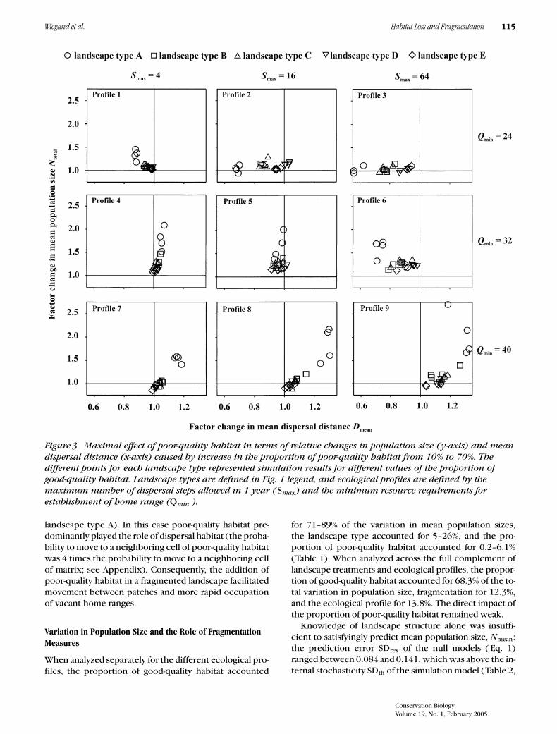
In fragmented landscapes (type A), mean population sizeresponded strongly to an increase in poor-quality habitatfrom fp = 0.1 to fp = 0.7 (Fig. 3). Mean population sizeincreased up to 2.7 times for ecological profile 9 and morethan 2 times for ecological profiles 4, 5, 8, and 9 (Fig.3). For all other landscape types, however, the maximalincrease was relatively moderate and reached factors of1.47 (B), 1.35 (C), and 1.27 (D and E).

The changes in population size resulting from the addi-tion of poor-quality habitat were accompanied by distinctchanges in mean dispersal distances. In one case popula-tion size increased and mean dispersal distance decreased(ecological profiles 1, 5, and 6 in landscape type A). This isbecause new sink home ranges were created and dispers-ing individuals had to cover less distance to encountera vacant home range. In a second case we observed theopposite effect: population size increased and dispersaldistance increased (ecological profiles 4, 7, 8 and 9 in



Figure 3. Maximal effect of poor-quality habitat in terms of relative changes in population size (y-axis) and meandispersal distance (x-axis) caused by increase in the proportion of poor-quality habitat from 10% to 70%. Thedifferent points for each landscape type represented simulation results for different values of the proportion ofgood-quality habitat. Landscape types are defined in Fig. 1 legend, and ecological profiles are defined by themaximum number of dispersal steps allowed in 1 year ( Smax) and the minimum resource requirements forestablishment of home range (Qmin ).

landscape type A). In this case poor-quality habitat pre-dominantly played the role of dispersal habitat (the proba-bility to move to a neighboring cell of poor-quality habitatwas 4 times the probability to move to a neighboring cellof matrix; see Appendix). Consequently, the addition ofpoor-quality habitat in a fragmented landscape facilitatedmovement between patches and more rapid occupationof vacant home ranges.


When analyzed separately for the different ecological pro-files, the proportion of good-quality habitat accounted

for 71–89% of the variation in mean population sizes,the landscape type accounted for 5–26%, and the pro-portion of poor-quality habitat accounted for 0.2–6.1%(Table 1). When analyzed across the full complement oflandscape treatments and ecological profiles, the propor-tion of good-quality habitat accounted for 68.3% of the to-tal variation in population size, fragmentation for 12.3%,and the ecological profile for 13.8%. The direct impact ofthe proportion of poor-quality habitat remained weak.

Knowledge of landscape structure alone was insuffi-cient to satisfyingly predict mean population size, Nmean:the prediction error SDres of the null models ( Eq. 1)ranged between 0.084 and 0.141, which was above the in-ternal stochasticity SDth of the simulation model (Table 2,



Table 2. Results of the two statistical models (Eqs. 1 & 2) that describe the results of the simulation model, reported separately for the nineecological profiles. a

Null model,b Eq. 1 Full statistical model,b Eq. 2Nmean = N0 fG + afp Nmean = N0 fG + aw fP + bw OGN + cw OGM

Ecological profile Internal model noise, SDth N0 ac SDres N0 aw bw cwc SDres

1 0.063 0.789 — 0.107 0.921 0.096 −0.31 — 0.0452 0.080 0.803 — 0.100 0.929 0.084 −0.286 — 0.0433 0.064 0.803 — 0.096 0.934 0.065 −0.273 — 0.0434 0.063 0.785 — 0.120 0.899 0.118 −0.267 −0.111∗ 0.0465 0.082 0.751 0.084∗ 0.090 0.879 0.123 −0.210 −0.079∗ 0.0366 0.069 0.729 0.100 0.084 0.837 0.168 −0.238 — 0.0397 0.067 0.746 — 0.141 0.98 — −0.302 −0.147 0.0608 0.081 0.840 — 0.094 1.000 −0.062 −0.066∗ −0.293 0.0319 0.058 0.875 — 0.092 0.994 −0.045 — −0.357 0.032

aDefinitions: Nmean, mean number of independent females between simulation years 100–200, averaged over the 20 replicate simulations; fG,proportion of good-quality habitat; fP, proportion of poor-quality habitat; OGN and OGM , fragmentation measures; N0, a, aw, bw, cw,coefficients of the statistical models; all dependent and independent variables were scaled to values between 0 and 1 to make the regressioncoefficients comparable between ecological profiles; SDth, internal noise of simulation model due to demographic stochasticity; SDres, predictionerror of statistical model (a statistical model described the results of the simulation satisfyingly if SDres < SDth).bModel selection was based on parsimony (lowest AIC) and simplicity (the simplest model among plausible models with �AIC <3).cProbability: ∗ 0.005 < p <0.05; in all other cases p < 0.005.

Fig. 4a). The most parsimonious full statistical models(Eq. 2) contained at least one fragmentation measure(Table 2) and yielded satisfactory statistical models thatexplained all variation in population size resulting fromlandscape structure within the limits set by demographicstochasticity (Table 2, Fig. 4b).

The coefficient aw of poor-quality habitat remained low(|aw| ≤ 0.17), indicating a weak direct effect on meanpopulation size, similar to that obtained with the analy-sis of variance (Table 1). The significant coefficients ofthe landscape measures OGN(3) and OGM(3) described anegative effect of fragmentation on population size. Inter-estingly, the coefficients bw and cw were negatively cor-related (Table 2, rp = −0.88, p = 0.002, n = 9), whichsuggests that OGN(3) and OGM(3) describe “competing”aspects of habitat fragmentation that dominate under dif-ferent biological circumstances.

Figure 4. The two (a and b)statistical models for ecologicalprofile 9 with high dispersal ability(Smax = 64) and scarce breedinghabitat (Qmin ). The graphs showpredicted values over observedvalues (the average populationsizes of the simulation model, bars,range of ± 1 SD taken from the 20replicate simulations). Solid linesshow the expected line for a perfectstatistical model, and dotted linesindicate the uncertainty of thesimulation model due to internalstochasticity (i.e., SDth = 0.058).

Maximal Fragmentation Effect

The maximal fragmentation effect was marked (Fig. 5)and when averaged over all ecological profiles and 16 dif-ferent landscape compositions, yielded a loss of half thepopulation (NA

mean/NEmean = 0.45 ± 0.21) (± SD). The

equivalent pure loss of (good-quality) habitat was equalto an area of 7% (± 2.6%) of the total landscape. In gen-eral, the maximal fragmentation effect was stronger forlandscapes with lower proportion of poor-quality habi-tat (gray circles in Fig. 5) and for ecological profiles withlower mean dispersal distance.

Ecological profiles 7 and 4 were most sensitive to maxi-mal habitat fragmentation, yielding an average equivalentloss of 10.0% (± 2.6%) and 9.2% (± 2.0), respectively.

The largest effects occurred when the proportion ofpoor-quality habitat was low (gray circles in Fig. 5). In



Figure 5. Maximal effect of habitat fragmentation assessed through comparison of mean population sizes inlandscapes of the contiguous type E and the highly fragmented type A (under constant composition). Graphs showthe equivalent (pure) loss of good-quality habitat �fG (Eq. 5) due to maximal fragmentation in dependence on thefactor decline NA

mean/NEmean (Qmin and Smax are defined in Fig. 3 legend, horizontal dashed lines indicate the

range of �fG).

these cases the dispersal ability was low and the habitatsuitable for home ranges was scarce, with females unableto reach vacant, but distant, home ranges. The maximalfragmentation effect occurred for ecological profile 7: afragmented landscape with fG = 0.25 and fp = 0.1 sus-tained approximately the same population size as a non-fragmented landscape with fG = 0.1 and fp = 0.1 (i.e.,an equivalent pure loss of 15% good-quality habitat). Ex-pressed as maximal decline in population size, the fac-tor change in population size (NA

mean/NEmean) reached a

value of 0.16 for ecological profile 7 in the landscapeswith fG = 0.1 and fp = 0.1.

Ecological profiles 8 and 9, with the highest mean dis-persal distances, showed a response to maximal fragmen-tation that ranged from no effect at all ( landscapes withabundant dispersal habitat, fp = 0.7) to a maximal de-crease in mean population size to approximately one-

fourth of the population size in the nonfragmented land-scape with the same composition ( fp = 0.1, and fG = 0.1)or an equivalent pure loss of 10% of good-quality habitat( fp = 0.1, and fG = 0.25). This result shows that abun-dant dispersal habitat can completely mitigate the effectof good-quality habitat fragmentation if the dispersal po-tential of the species is sufficiently large (cf. ecologicalprofiles 8 and 9 in Fig. 5). In this case the landscape isfunctionally connected and population dynamics are thatof a spatially structured population.

Discussion


Our study is among the first investigations that use threehabitat types (good-quality habitat, poor-quality habitat,



and matrix) to assess the traditional approach of usingtwo habitat types only (habitat and matrix). The tradi-tional habitat–matrix approximation did not hold whenpoor-quality habitat provided sink habitat in the neighbor-hood of highly fragmented good-quality habitat or whenpoor-quality habitat provided dispersal habitat, enhanc-ing movement between patches of highly fragmentedbreeding habitat. In both cases, the “error” of not con-sidering poor-quality habitat could have the effect ofmore than doubling the predicted population size (Fig.3). The first case is well conceptualized and follows di-rectly from source-sink theory (Pulliam 1988; Pulliam &Danielson 1991). The second case, however, has impor-tant implications for conservation because increasing theamount of poor-quality habitat in a landscape can be in-terpreted as a successful conservation measure to im-prove matrix quality—dispersal mortality decreased andthe restored habitat enhanced dispersal between patchesof fragmented breeding habitat. Restoring larger propor-tions of the matrix (e.g., by restoring landscape struc-tures that increase the survival of dispersers by providingshelter from predators or food sources) might be eco-nomically cheaper and ecologically easier than restoringbreeding habitat.

The second case also has important implications fortheoretical studies on fragmentation. It suggests that dis-persal habitat matters most for species with intermedi-ate dispersal abilities living in landscapes composed ofsmall patches of breeding habitat in which dispersal habi-tat can enhance the occasional exchange of individualsbetween patches (i.e., a metapopulation or a spatiallystructured population). Thus, theoretical metapopulationstudies need to explicitly consider dispersal habitat in-stead of using the more traditional binary habitat–matrixapproximation. The effect of landscape heterogeneity ondispersal, however, is complex and difficult to analyze andmeasure because the uniqueness of each landscape andthe complex interactions of effects will always confoundsimple analysis (Gustafson & Gardner 1996; Moilanen &Hanski 1998). Dispersal habitat introduces an additionaldegree of freedom in possible landscape configurationsthat may lead to completely different structural connec-tivity values for landscapes with the same configuration ofgood-quality habitat patches but different configurationsand proportions of dispersal habitat. This has resulted inmetapopulation studies generally ignoring matrix hetero-geneity (Wiens et al. 1993; Gustafson & Gardner 1996;Wiegand et al. 1999).

Nonetheless, a few theoretical studies address the ef-fect of matrix heterogeneity (e.g., Gustafson & Gard-ner 1996; Moilanen & Hanski 1998) or matrix qual-ity (e.g., Fahrig 2001; Vandermeer & Carvajal 2001) on(meta)population dynamics. Our finding that the overalleffects of fragmentation and matrix heterogeneity on pop-ulation size can be well described by two fragmentationmeasures with clear biological interpretations is an im-portant step for obtaining a more general understanding

of this issue. One fragmentation measure, OGN(rcrit), cap-tures patch-size effects of good-quality habitat patches at acritical scale, rcrit, and contributes significantly to the abil-ity to predict population sizes for species with low disper-sal ability: in landscapes with lower values of OGN(rcrit),more home ranges are situated at the edge of good-qualityhabitat patches. Consequently, the mean habitat suitabil-ity of such “edge” home ranges is lower and the risk ofmortality higher. This patch-size effect is usually not con-sidered in theoretical studies.

The second fragmentation measure, OGM(rcrit), cap-tures patch isolation effects at a critical scale rcrit andcontributes significantly to predict population sizes forspecies with intermediate dispersal ability. The OGM(rcrit)differs substantially from other measures of patch isola-tion (e.g., Vos et al. 2001) because it considers the struc-ture of dispersal habitat and uses a critical scale, rcrit, thatis independent of maximal (or average) dispersal distance(Wiegand et al. 1999, Eq. 8 and Fig. 12). The OGM(rcrit)correctly described fragmentation effects for landscapeswith three types of habitat and species with intermediatedispersal ability (ecological profiles 8 and 9). This find-ing is a promising starting point for future investigationinto generalizing different dispersal rules and landscapestructures. The need for this is documented in a grow-ing body of empirical studies that provide evidence forthe importance of matrix heterogeneity during dispersal(e.g., Delin & Andren 1999; Palomares et al. 2000; Reuna-nen et al. 2000; Ricketts 2001; Revilla et al. 2004).


As expected, the proportion fG of good-quality habi-tat was the strongest predictor of population size (e.g.,Andren 1994, 1996), but figures were notably below the>96% found by Flather and Bevers (2002) in a similarstudy. The main reason for this difference is the differ-ent range of habitat proportion considered (0.1−0.9 inFlather & Bevers [2002]). Flather and Bevers (2002), how-ever, analyzed a “below threshold condition” (definedthrough a persistence threshold of habitat amount) thatinvolved a narrower range of habitat amounts. For thissubset of landscapes, they found that habitat amount ac-counted for between 30% and 52% of the variation inpopulation size. This figure is in better agreement withour results, which suggest that the overpowering effectof habitat amount is considerably reduced if habitat lossis placed in a perspective of realistic habitat proportionsand losses and in a broader perspective of varying speciesattributes. We argue that the response of a population tohabitat fragmentation may in general not be straightfor-ward but strongly dependent on species-specific proper-ties.

An additional reason for stronger impacts of habitatfragmentation in our study compared with the results ofother studies (e.g., McGarigal & McComb 1995; Fahrig



1997, 1998, 2001; Trzcinski et al. 1999; Flather & Bev-ers 2002) are differences in the species groups consid-ered. Long-lived species with stable home ranges and na-tal dispersal may be more vulnerable to effects of habitatfragmentation. A recent study on the habitat quality ofbrown bears in northern Spain (Naves et al. 2003) sug-gests that habitat suitability varies considerably at a spatialscale slightly smaller than a home range. Home ranges atthe edge of good-quality habitat patches could comprisepoor-quality habitat areas that decrease the overall suit-ability of the home range and may increase the risk ofmortality. This fragmentation effect was important in oursimulation model but not included in more simple mod-els for hypothetical species (e.g., Fahrig 1997; Flather &Bevers 2002).

Earlier attempts to explain variation in response vari-ables of population dynamics (mostly dispersal success)with measures of landscape composition and structurehave not been particularly successful (e.g., Gustafson &Gardner 1996; Schumaker 1996; Tischendorf 2001). Evenwhen considering a fully realized deterministic popu-lation model, Flather and Bevers (2002) failed to finddescriptors of landscape structure that satisfactorily ac-counted for the variation in population size introducedby altering landscape structure. They attributed the unex-pected high magnitude of unexplained variation in popu-lation response to the absence of appropriate variablesthat captured patch isolation effects. Notably, our fullstatistical model ( Eq. 2) yielded for all ecological pro-files a satisfying statistical model with a prediction errornot larger than the limit set by demographic stochasticity.This result increases our confidence in our approach oflandscape measures, which differs from that usually taken(e.g., McGarigal & Marks 1995; Gustafson 1998; Flather& Bevers 2002).

The Maximal Fragmentation Effect

Maximal fragmentation effects were strong, yielding onaverage a population decline to half of its size comparedwith population sizes in the unfragmented landscapewith the same composition. Maximal effects were equiva-lent to a pure loss of 15% good-quality habitat and a dropin population size to 16% of the population size in thecorresponding unfragmented landscape. In a metapopu-lation situation (when breeding habitat was scarce, eco-logical profiles 8 and 9), we found large variations inthe maximal fragmentation effect caused by variation inthe proportion of poor-quality habitat. If the landscapeswere functionally connected (i.e., abundant poor-qualityhabitat facilitated the exchange of individuals betweenpatches of fragmented breeding habitat), fragmentationhad no effect at all, whereas the maximal fragmentation ef-fects were large in functionally disconnected landscapeswith little poor-quality habitat.

Our findings suggest that predicting fragmentation ef-fects (and thus designing appropriate conservation mea-sures) requires a good understanding of the biology andhabitat use of the species in question. A change in criticalspecies-specific characteristics, such as dispersal abilityor use of dispersal habitat, altered the response of modelspecies to fragmentation completely, from no change atall to a loss of 80% of the individuals. The uniqueness ofspecies and landscapes in which they live will always con-found simple analysis. Therefore, it is not surprising thatcurrent theoretical studies in which simple models for hy-pothetical species were applied have been characterizedby a considerable degree of ambiguity (e.g., Fahrig 1997,1998, 2001; Hill & Caswell 1999; Hiebeler 2000; Flather& Bevers 2002).

Phenomenological models are often effective in help-ing to discern whether or not a particular type of effectis occurring in a system. Ecological systems, however, es-pecially those involving habitat loss and fragmentation,are complex and such models may not help elucidate thecausal chains by which the effect operates. Our approachof carefully providing more biological realism has the ad-vantage that it makes more model assumptions explicit.The concept of ecological profiles allowed us to track andexplain the differences in model outcome over a rangeof species characteristics, whereas such a comparisonbetween simple models with different assumptions andformulations is difficult. The comparison of our resultsamong differing species characteristics should make ourstudy useful as a starting point for future investigations.There is no reason to expect that the response of otherspecies groups to fragmentation may be less critically in-fluenced by species-specific characteristics. The variabil-ity in outcome we found, however, should not be takenas a source of frustration over the failure to generalize,but as a motivation for further research.

Acknowledgments

Funding provided by the UFZ-Centre for EnvironmentalResearch, Leipzig, and Iowa State University enabled theauthors to travel between Germany, the United States,and Spain for cooperative work. E. R. was supported by aMarie Curie Fellowship provided by the European Com-munity (Contract EVK2-CT-1999-50001). We thank J. Bas-compte, F. Knauer, J. Naves, K. Wiegand, C. Wissel, H.Possingham, and especially two anonymous reviewers forassistance during the development of ideas or for com-ments on drafts of this manuscript.

Literature Cited

Andren, H. 1994. Effects of habitat fragmentation on birds and mam-mals in landscapes with different proportion of suitable habitat—areview. Oikos 71:355–366.



Andren, H. 1996. Population responses to habitat fragmentation: statis-tical power and the random sample hypothesis. Oikos 76:235–242.

Bascompte, J., and R. V. Sole. 1996. Habitat fragmentation and extinctionthresholds in spatially explicit models. Journal of Animal Ecology65:465–473.

Bender, D. J., T. A. Contreras, and L. Fahrig. 1998. Habitat loss andpopulation decline: a meta-analysis of the patch size effect. Ecology79:517–533.

Boswell, G. P., N. F. Britton, and N. R. Franks. 1998. Habitat fragmenta-tion, percolation theory and the conservation of a keystone species.Proceedings of the Royal Society of London B, Biological Sciences265:1921–1925.

Delin, A. E., and H. Andren. 1999. Effects of habitat fragmentation onEurasian red squirrel (Sciurus vulgaris) in a forest landscape. Land-scape Ecology 14:67–72.

Dunning, J. B., D. J. Stewart, B. J. Danielson, B. R. Noon, T. L. Root, R.H. Lamberson, and E. E. Stevens. 1995. Spatially explicit populationmodels: current forms and future uses. Ecological Applications 5:3–11.

Fahrig, L., and G. Merriam. 1994. Conservation of fragmented popula-tions. Conservation Biology 8:50–59.

Fahrig, L. 1997. Relative effects of habitat loss and fragmentation onpopulation extinction. Journal of Wildlife Management 61:603–610.

Fahrig, L. 1998. When does fragmentation of breeding habitat affectpopulation survival? Ecological Modelling 105:273–292.

Fahrig, L. 2001. How much habitat is enough? Biological Conservation100:65–74.

Flather, C. H., and M. Bevers. 2002. Patchy reaction-diffusion and pop-ulation abundance: the relative importance of habitat amount andarrangement. The American Naturalist 159:40–56.

Forman, T. T. 1996. Land mosaics. The ecology of landscapes and re-gions. Cambridge University Press, New York.

Gaona, P., P. Ferreras, and M. Delibes. 1998. Dynamics and viability ofa metapopulation of the endangered Iberian Lynx (Lynx pardinus).Ecological Monographs 68:349–370.

Gustafson, E. J. 1998. Quantifying landscape spatial pattern: what is thestate of the art? Ecosystems 1:143–156.

Gustafson, E. J., and R. H. Gardner. 1996. The effect of landscape hetero-geneity on the probability of patch colonization. Ecology 77:94–107.

Hiebeler, D. 2000. Populations on fragmented landscapes with spatiallystructured heterogeneities: landscape generation and local dispersal.Ecology 81:1629–1641.

Hill, M. F., and H. Caswell. 1999. Habitat fragmentation and extinctionthresholds on fractal landscapes. Ecology Letters 2:121–127.

McGarigal, K. J., and B. J. Marks. 1995. FRAGSTATS: spatial pattern anal-ysis program for quantifying landscape structure. General TechnicalReport PNW-GTR-351, U.S. Department of Agriculture Forest Ser-vice (USFS), Pacific Northwest Research Station, Portland, Oregon.

McGarigal, K. J., and W. C. McComb. 1995. Relationships between land-scape structure and breeding birds in the Oregon coast range. Eco-logical Monographs 65:235–260.

McKelvey, K., B. R. Noon, and R. H. Lamberson. 1993. Conservationplanning for species occupying fragmented landscapes: the case ofthe northern spotted owl. Pages 424–450 in P. Kareiva, J. G. King-solver, and R. B. Huey, editors. Biotic interactions and global change.Sinauer, Sunderland, Massachusetts.

Moilanen, A., and I. Hanski. 1998. Metapopulation dynamics: effects ofhabitat quality and landscape structure. Ecology 79:2503–2515.

Naves, J., T. Wiegand, E. Revilla, and M. Delibes. 2003. Endangeredspecies balancing between natural and human constrains: the caseof brown bears (Ursus arctos) in northern Spain. Conservation Bi-ology 17:1276–1289.

Noss, R. F., and B. Csuti. 1997. Habitat fragmentation. Pages 269–304in G. K. Meffe and C. R. Carroll, editors. Principles of conservationbiology. 2nd edition. Sinauer, Sunderland, Massachusetts.

Palomares, F., M. Delibes, P. Ferreras, J. Fedriani, J. Calzada, and E. Re-villa. 2000. Iberian lynx in a fragmented landscape: pre-dispersal,

dispersal and post-dispersal habitats. Conservation Biology 14:809–818.

Pulliam, H. R. 1988. Sources, sinks, and population regulation. TheAmerican Naturalist 132:652–661.

Pulliam, H. R., and B. J. Danielson. 1991. Sources, sinks, and habitat se-lection: a landscape perspective on population dynamics. The Amer-ican Naturalist 137:S50–S66.

Reunanen, P., M. Monkkonen, and A. Nikula. 2000. Managing borealforest landscapes for flying squirrels. Conservation Biology 14:218–226.

Revilla, E., T. Wiegand, F. Palomares, P. Ferreras, and M. Delibes. 2004.Modeling individual dispersal movement in real landscapes: the im-portance of structural realism. The American Naturalist 164:E130–E153.

Ricketts, T. H. 2001. The matrix matters: effective isolation in frag-mented landscapes. The American Naturalist 158:87–99.

Schumaker, N. H. 1996. Using landscape indices to predict habitat con-nectivity. Ecology 77:1210–1225.

Soule, M. E. 1986. Conservation biology: the science of scarcity anddiversity. Sinauer, Sunderland, Massachusetts.

Tischendorf, L. 2001. Can landscape indices predict ecological pro-cesses consistently? Landscape Ecology 16:235–254.

Trzcinski, M. K., L. Fahrig, and G. Merriam. 1999. Independent effects offorest cover and fragmentation on the distribution of forest breedingbirds. Ecological Applications 9:586–593.

Vandermeer, J., and R. Carvajal. 2001. Metapopulation dynamics andthe quality of the matrix. The American Naturalist 158:211–20.

Vos, C. C., J. Verboom, P. F. M. Opdam, and C. J. F. Ter Braak. 2001. To-ward ecologically scaled landscape indices. The American Naturalist157:24–41.

Wiegand, T., K. A. Moloney, J. Naves, and F. Knauer. 1999. Finding themissing link between landscape structure and population dynam-ics: a spatially explicit perspective. The American Naturalist 154:605–627.

Wiegand, T., J. Naves, T. Stephan, and A. Fernandez. 1998. Assessing therisk of extinction for the brown bear (Ursus arctos) in the CordilleraCantabrica, Spain. Ecological Monographs 68:539–570.

Wiens, J. A., N. C. Stenseth, B. Van Horne, and R. A. Ims. 1993. Ecologicalmechanisms and landscape ecology. Oikos 66:369–80.

Appendix

The demographic submodel is a simplified version of a nonspatial de-mographic model for brown bears in northern Spain (Wiegand et al.1998). We did not include subadult and adult males because we wereinterested in the aspects of population dynamics that are primarily de-termined by females. The parameters of the demographic submodel arelisted in Wiegand et al. (1999, Table 1), but mortality rates are modi-fied by local habitat quality. Mortality rates were adjusted to produce anoverall rate of population increase of λ > 1.03 (λ < 0.99) for landscapesconsisting completely of good- (poor-) quality habitat (Wiegand et al.1999, Fig. 6).

We distinguished between habitat quality Z and habitat suitabilityQ. Habitat quality was defined by the landscape maps (good-qualityhabitat, Z = 7; poor-quality habitat, Z = 4; and matrix, Z = 1). Habitatsuitability Q was reduced when a cell was shared by several females ashome range, and was Z = Q otherwise. The habitat suitability of a cell ofgood or poor-quality habitat dropped to 5, 3, 2, or 3, 2, 1, respectively,if two, three, or four females shared the cell as home range.

Independent, nonresident females dispersed and searched for a homerange. We modeled sequential dispersal from multiple natal sites withcompetition between residents and dispersers by first selecting the old-est female and continuing in order of decreasing age. During 1 year,dispersing females were allowed to perform Smax site-sampling steps.They moved one grid cell per step, and the cell to which they moved wasselected with a probability that was directly proportional to the habitat



suitability Q of the cell, relative to that of the other eight cells of the 3 ×3 cell area surrounding the present location. Movement continued untilthe dispersing female found a home range, until the maximal numberof dispersal steps was reached, or until she died.

Mortality during dispersal was considered in addition to age-dependent mortality (see below) as a per-step probability of dying, de-fined as (1 − Qm/9)/Rmax, where Qm was the mean habitat suitabilityof the 3 × 3 cell neighborhood, determined after accounting for den-sity effects, and Rmax = 400 was a scaling constant (see Wiegand et al.1999).

A dispersing female established a home range if the total habitatsuitability of the 3 × 3 cell area surrounding its present location ex-ceeded the minimal resource requirements Qmin. The home range wasthe collection of the highest quality cells that, as a whole, exceededthe threshold Qmin. Resident females stayed in their home range un-til death, even if the total habitat suitability of the home range tem-porarily dropped below the threshold Qmin after a newcomer settlednearby.

Only females occupying an own home range could reproduce. Wedid not consider different probabilities for litter production in homeranges with different habitat qualities; instead, we varied cub mortalityin accordance with the habitat quality of the mother’s home range.Similarly, we did not consider variability in reproduction as a functionof habitat quality because the rate of increase of a brown bear populationis much more sensitive to mortality rates than to reproduction (Wiegandet al. 1998).

We multiplied the age-dependent mortality rates (given in Wiegandet al. 1999, Table 1) with the factor [1 − cm(1 − QHR/4)], where QHR

is the mean habitat quality of the home range and cm = 0.35, a scalingconstant (Wiegand et al. 1999) that determined the magnitude of theimpact of habitat suitability on mortality. Mortality applied to each in-dividual independently. For dependent cubs we used the mean habitatquality QHR of their mother’s home range; for resident females (includ-ing successful dispersers of the year), we used the QHR of their ownhome range; and for dispersers that did not find a home range, we ap-plied a mortality rate that corresponds to QHR = 4.


effects of habitat loss and fragmentation on population...

Documents