effects of climate variability and land use change - … · effects of climate variability and land...
TRANSCRIPT


Effects of climate variability and land use change
on the water budget of large river basins
Ruud T.W.L. Hurkmans

Promotoren:
Prof. dr. ir. P.A. Troch Hoogleraar Hydrologie en Kwantitatief Waterbeheer,
Wageningen Universiteit (1999–2005).
Professor of Hydrology and Water Resources,
Professor of Civil Engineering and Engineering Mechanics,
University of Arizona, USA.
Prof. dr. ir. R. Uijlenhoet Hoogleraar Hydrologie en Kwantitatief Waterbeheer,
Wageningen Universiteit
Promotiecommissie:
Prof. dr. ir. M.F.P. Bierkens Universiteit Utrecht
Prof. dr. B.J.J.M. van den Hurk Universiteit Utrecht en KNMI, De Bilt
Dr. D. Jacob Max Planck Institut fur Meteorologie, Hamburg, Duitsland
Prof. dr. P. Kabat Wageningen Universiteit
Dit onderzoek is uitgevoerd binnen de onderzoeksschool WIMEK-SENSE.

Effects of climate variability and land use change
on the water budget of large river basins
Ruud T.W.L. Hurkmans
Proefschrift
ter verkrijging van de graad van doctor
op gezag van de rector magnificus
van Wageningen Universiteit,
Prof. dr. M.J. Kropff,
in het openbaar te verdedigen
op maandag 15 juni 2009
des namiddags te half twee in de Aula.

Hurkmans, R.T.W.L.
Effects of climate variability and land use change on the water budget of large river basins [Ph.D.
thesis, Wageningen University, 2009, xviii+174 pp.]
In Dutch: Effecten van klimaatvariabiliteit en landgebruiksverandering op de waterhuishouding van
stroomgebieden van grote rivieren. [proefschrift, Wageningen Universiteit, 2009, xviii+174 pp.]
ISBN 978-90-8585-398-5
Abstract
Due to global warming, the hydrologic behavior of the Rhine basin is expected to shift from a com-
bined snowmelt and rainfall driven regime to a more rainfall dominated regime. Land use changes
may reinforce the effects of this shift through urbanization, or counteract them through, for example,
afforestation. One of the objectives of this thesis is to investigate and quantify these changes in the
hydrological regime of the Rhine basin using hydrological modeling studies. The Variable Infiltra-
tion Capacity (VIC) model is used throughout this thesis as the hydrological model. Designed as a
land surface model, the VIC model’s physically-based formulation for land-atmosphere interactions
offers the potential to more accurately simulate the partitioning of precipitation into evapotranspira-
tion and streamflow compared to more simple water balance models. This potential is investigated
by comparing the accuracy of streamflow simulations of the water balance model (STREAM) and the
VIC model. Both models are applied to the Rhine river basin using downscaled re-analysis data as
atmospheric forcing, and evaluated using observed streamflow and lysimeter data. We find that VIC
is more robust and less dependent on model calibration. Whereas STREAMmore effectively compen-
sated for erroneous forcing data in the calibration period, VIC performed better than STREAM in the
validation period, except for the Alpine part where both models have difficulties due to the complex
terrain and surface reservoirs.
Subsequently, the VIC model is used to investigate the effects of projected land use change scenarios
on mean and extreme river discharge in the Rhine basin at various spatial scales. Atmospheric forc-
ing is kept constant and consists of the downscaled re-analysis data mentioned before. To simulate
differences between vegetation types realistically, the model is modified to allow for bare soil evap-
oration and canopy evapotranspiration simultaneously in sparsely vegetated areas, as this is more
appropriate to simulate seasonal effects. All projected land use change scenarios lead to an increase
in streamflow. Streamflow at the basin outlet proved rather insensitive to land use changes, because
over the entire basin affected areas are relatively small. Moreover, projected land use changes (ur-
banization and conversion of cropland into (semi-)natural land or forest) have opposite effects. At
smaller scales, however, the effects can be considerable. In addition, the effects of climate change on
Rhine river discharge are evaluated, keeping the land use constant. High-resolution (0.088◦) regional
climate scenarios are used to force the VIC model. These climate scenarios are based on model output
from the ECHAM5-OM global climate model, which is in turn forced by three SRES emission scenar-
vii

ios: A2, A1B and B1. Average streamflow, peak flows, low flows and several water balance terms are
evaluated for both the first and second half of the 21st century. The first half of the century appears
to be dominated by increased precipitation and streamflow throughout the year. During the second
half of the century, a streamflow increase in winter/spring and a decrease in summer is found, sim-
ilar to previous studies. Magnitudes of peak flows increase during both periods, that of streamflow
droughts only during the second half of the century.
Another source of climate variability are interannual cycles of sea surface temperature, which influ-
ence the global climate through teleconnections. In the Colorado river basin, which has been experi-
encing extremely dry conditions during recent years, such teleconnections have been shown to have
a significant influence on precipitation and streamflow. Time series of terrestrial water storage com-
ponents, precipitation and discharge spanning 74 years are extracted from a simulation using the VIC
model and related to climate indices that describe the variability of sea surface temperature and sea
level pressure in the tropical and extra-tropical Pacific Ocean. Especially the low-frequency mode of
the Pacific Decadal Oscillation (PDO) appears to be strongly correlated with deep soil moisture stor-
age and surface water reservoir storage. During the negative PDO phase, these storage anomalies
tend to be negative, and the “amplitudes” (mean absolute anomalies) of soil moisture, snow and dis-
charge are lower compared to periods having positive PDO phases. If indeed a shift to a cool PDO
phase occurred in at the end of the nineties, as data suggest, the current dry conditions in the Col-
orado basin may persist.
Finally, a distinguishing feature of the VIC model, its parameterization for small-scale heterogeneity
in soil moisture variability is compared with alternative parameterizations in a small, Alpine sub-
catchment of the Rhine, the Rietholzbach. As an alternative for the VIC parameterization, a hillslope-
based parameterization is developed and compared to TOPMODEL and the VIC model. The effect
of hillslope exposure on the resulting discharge is generally larger than that of spatial aggregation,
although differences do occur in the generation of surface runoff. These are, however, generally com-
pensated by decreasing baseflow. The changes in discharge are, therefore, small. Reduction of the
amount of hillslopes in the catchment by classification based on hillslope similarity parameters yields
similar results as when modeling individual hillslopes explicitly, which is much less the case when
the catchment is modeled as an “open-book” or one large hillslope. Because the slopes in the Ri-
etholzbach are generally steep, the influence of groundwater on soil moisture variability is relatively
small and the VIC model is found to be able to accurately model catchment-averaged evapotranspi-
ration and discharge.
viii

Voorwoord / Preface
Voor u ligt het resultaat van ruim vier jaar promotie-onderzoek. Bij het tot stand komen van een
proefschrift zijn natuurlijk veel meer mensen betrokken dan alleen ik, vandaar een woord van dank.
Allereerst wil ik Peter Troch bedanken voor het mij er toe aanzetten uberhaupt met promoveren te
beginnen. Het eindgesprek van mijn afstudeervak (over een totaal ander onderwerp) eindigde met
“en misschien kunnen we later nog eens wat samen onderzoeken”. Enkele jaren later was het dan
zover; in september 2004 begon ik als AIO bij de leerstoelgroep Hydrologie & Kwantitatief Waterbe-
heer. Toen ik eenmaal op gang gekomen was nam Peter eind 2005 helaas de benen om naar Tucson,
Arizona, te verhuizen. Ondanks het feit dat begeleiding via email en telefoon toch niet altijd even
efficient bleek als “live” met elkaar te kunnen praten, pakte het allemaal goed uit. Ook bood het een
mooie kans om een tijdje in Tucson te verblijven, waar ik twee keer enkele maanden dankbaar ge-
bruik van heb gemaakt. Peter, bedankt voor dat alles, en ook de gastvrijheid waarmee ik in Tucson
ontvangen werd. Also the people in Peter’s group: Maite, Steve, Matt: thanks for all your help in
finding apartments, the lunches, the discussions and the fun. Matej, thanks for your help while I was
in Tucson and for always promptly sending all kinds of data when requested.
Weer terug in Nederland werd Remko Uijlenhoet de nieuwe hoogleraar. Remko, ik ben erg blij dat
je mij als enigszins “verweesde” AIO onder je hoede hebt genomen. Ondanks de grote hoeveelheid
andere AIO’s maakte je tijd; bedankt voor de inspirerende gesprekken en voor de (wanneer dat nodig
was) pragmatische manier van beslissingen nemen. Ook de andere collega’s bij de leerstoelgroepen
Hydrologie en Kwantitatief Waterbeheer en Bodemfysica, Ecohydrologie en Grondwaterbeheer: be-
dankt voor de gezellige en inspirerende lunches en koffiepauzes, en het elk jaar weer erg geslaagde
weekje EGU in Wenen. In het bijzonder Hidde, Patrick en Paul: bedankt voor het altijd klaarstaan
om allerlei Matlab-, LaTeX- of willekeurige andere probleempjes te helpen oplossen. Eind 2007 werd
Wilco Terink aangesteld op een sterk gerelateerd project, waardoor hij ook nauw betrokken was bij
enkele hoofdstukken van dit proefschrift. Wilco, bedankt voor de prettige samenwerking! Verder ben
ik Eddy Moors van de leerstoelgroep Aardsysteemkunde, die betrokken was via hetzelfde project,
erg dankbaar voor de waardevolle discussies en suggesties. Ook Peter Verburg van de leerstoel-
groep Landdynamiek wil ik graag bedanken voor het beschikbaarstellen van de landgebruiksveran-
deringsscenarios en de waardevolle feedback op Hoofdstuk 3.
ix

Ook buiten de universiteit zijn er veel mensen die hun data voor mij beschikbaar stelden, en/of met
wie ik mocht samenwerken. Hoofdstuk 2 is voor een belangrijk deel tot stand gekomen met de hulp
van Jeroen Aerts en Hans de Moel van de Vrije Universiteit Amsterdam: bedankt daarvoor! De at-
mosferische data die in vrijwel het hele proefschrift werd gebruikt is afkomstig van het Max Planck
Institut fur Meteorologie in Hamburg. FromMPI-M, I’d like to thank Daniela Jacob for making avail-
able the climate model data and for the very nice and useful discussions we had in Hamburg, and
Eva Starke for helping in using the data. Hendrik Buiteveld en Rita Lammersen van (tegenwoordig)
Rijkswaterstaat Waterdienst, bedankt voor het beschikbaar stellen van alle geobserveerde data. Fur-
thermore, I would like to thank Irene Lehner and Reto Stockli from ETH Zurich for providing data
from the Rietholzbach catchment.
In 2006 kreeg ik samen met Ryan Teuling, dankzij een reisbeurs van NWO, de kans om deel te nemen
aan een veld-experiment in Australie. Ondanks het feit dat de resulterende data uiteindelijk niet in
dit proefschrift terecht gekomen zijn was het een fantastische ervaring. Jeff, Rocco, Olivier and all the
other participants of the NAFE campaign, thanks for the great time!
Tegen het einde van mijn AIO-periode kreeg ik de gelegenheid twee studenten (mede) te begeleiden.
Marcel en Tjeerd, het was een genoegen om jullie te begeleiden en ik heb er zelf ook veel van geleerd.
Tot slot, voor iedereen die heeft bijgedragen aan dit boekje maar hierboven niet genoemd is: hartelijk
bedankt!
Het is natuurlijk onmogelijk om almaar aan een proefschrift te werken; de ontspanning tussendoor
is ook erg belangrijk. Ik heb altijd met veel plezier bij de Ontzetting gespeeld, en later ook bij allerlei
andere orkesten in de buurt. (oud)-Ontzetters, bedankt voor alle gezelligheid! In hetzelfde kader wil
ik ook de (ex-)bewoners van Haarweg 217, waar ik altijd erg prettig gewoond heb, en het clubje van
oud-roeiers bedanken. Bart en Pieter, leuk dat jullie mijn paranimfen willen zijn! Rest mij nog mijn
ouders, Carin en Paul te bedanken voor alle kansen die zij mij geboden hebben. Tenslotte, Rinske:
voor mij zit het er bijna op, voor jou breken de laatste loodjes nu aan. Hopelijk heb jij in de komende
tijd net zoveel aan mij als ik aan jou heb gehad!
Ruud
x

Acronyms and abbreviations used in this thesis
A1 SRES scenario type: “global economy”
A1B SRES scenario type: “global economy with balanced energy sources”
A2 SRES scenario type: “continental market”
B1 SRES scenario type: “global cooperation”
B2 SRES scenario type: “regional communities”
CATHY Catchment Hydrological model
CHR International Commission for the Hydrology of the Rhine
CRB Colorado River Basin
DEM Digital Elevation Model
E Nash-Sutcliffe modeling efficiency
ECHAM5-OM Global climate model developed by MPI-M
ECMWF European Centre for Medium-range Weather Forecasting
ENSO El Nino Southern Oscillation
ERA ECMWF re-analysis
ERA15 ECMWF re-analysis dataset (1979-1993)
ERA15d Downscaled ERA15-data
ESMA Explicit Soil Moisture Accounting models
FAO United Nations Food and Agriculture Organisation
GEV Generalized Extreme Value distribution
GCM Global Climate Model
GHG Greenhouse gas
GIS Geographical Information System
GP Generalized Pareto distribution
HBV Hydrologiska Byrans Vattenbalansavdelning model
hsB hillslope-storage Boussinesq model
hsB-LATS hsB, coupled to an unsaturated zone model
IPCC Intergovernmental Panel on Climate Change
LAI Leaf Area Index
LPJ Lund-Potsdam-Jena global vegetation model
LSM Land surface model
xi
MEI Multi-variate ENSO index
MPI-M Max Planck Institut fur Meteorologie, Hamburg, Germany
NINO34 Index describing ENSO variability
NINO3 Index describing ENSO variability
NINO4 Index describing ENSO variability
NINO12 Index describing ENSO variability
PDM Probability Distributed Model
PDO Pacific Decadal Oscillation
PDV Pacific Decadal Variability
PELCOM Pan-European Land Cover Monitoring and Mapping
PNA Pacific North-American pattern
MAMQ Average annual maximum streamflow
Max Q Maximum river streamflow
Mean Q Average river streamflow
RCM Regional Climate Model
REMO Regional climate model developed by MPI-M
RVE Relative Volume Error
SHE Systeme Hydrologique Europeen; physically based hydrological model
SRES Special Report on Emissions Scenarios
SST Sea Surface Temperature
STREAM Spatial tools for river basins and environment and analysis of management options model
SVAT Soil-Vegetation-Atmosphere-Transfer
SWE SnowWater Equivalent
TOPMODEL Topographic-index based hydrological model
TOPLATS Land surface model based on TOPMODEL
TWS Terrestrial Water Storage
USDA United States Department of Agriculture
VIC Variable Infiltration Capacity model
xii

Contents
1 General introduction 1
1.1 Background 3
1.1.1 Hydrological modeling 3
1.1.2 Climate variability and climate change 5
1.1.3 Greenhouse gas emission scenarios 8
1.2 Study area 9
1.3 The Variable Infiltration Capacity model 12
1.3.1 Streamflow generation 12
1.3.2 Evapotranspiration 14
1.3.3 Streamflow routing 15
1.4 Problem description and thesis outline 15
2 Water balance versus land surface model in the simulation of Rhine river discharges 19
2.1 Introduction 21
2.2 Study area and data 22
2.3 Description of models 25
2.4 Model calibration 28
2.5 Model validation 30
2.6 Discussion and conclusions 38
3 Effects of land use changes on streamflow generation in the Rhine basin 41
3.1 Introduction 43
3.2 Study area, model and data 44
3.3 VIC model simulations of a single pixel 49
3.4 VIC model simulations for the entire basin 55
3.5 Summary and conclusions 61
xiii

4 Changes in streamflow in the Rhine basin under climate scenarios 65
4.1 Introduction 67
4.2 Data and model 68
4.2.1 Study area 68
4.2.2 Hydrological model 69
4.2.3 Atmospheric data 69
4.3 Methodology 71
4.3.1 Bias correction 71
4.3.2 Model calibration 74
4.4 Results 75
4.4.1 Spatial patterns of atmospheric variables 76
4.4.2 Mean streamflow 79
4.4.3 Water balance components 80
4.4.4 Extreme streamflow 83
4.5 Discussion 87
4.6 Conclusions 90
5 Effects of climate variability on water storage in the Colorado River Basin 91
5.1 Introduction 93
5.2 Study area and datasets 94
5.3 Results 98
5.3.1 Analysis of spatial averages 98
5.3.2 Analysis of distributed data 104
5.4 Summary and conclusions 107
6 A hillslope-based parameterization for sub-grid variability of topography 109
6.1 Introduction 111
6.2 Study area and data 112
6.3 Hydrological models 113
6.3.1 TOPMODEL 115
6.3.2 The hillslope-storage Boussinesq model 116
6.3.3 Unsaturated zone formulation 116
6.4 Methodology 119
6.4.1 Correction for hillslope exposure 120
6.4.2 Hillslope delineation and classification 122
6.5 Results 124
6.6 Summary and conclusions 132
7 General discussion 135
7.1 Introduction 137
7.2 Discussion of the hydrological model 137
xiv

7.3 Discussion of the climate and land use change scenarios 138
7.4 General conclusions 139
7.4.1 Effects of land use change 140
7.4.2 Effects of climate change 140
7.4.3 Effects of oscillations in ocean temperature 141
7.4.4 An alternative parameterization for small-scale variability of soil moisture 142
7.5 Directions for further research 142
8 Nederlandse samenvatting 145
8.1 Inleiding 147
8.2 Het hydrologisch model in perspectief 147
8.3 De landgebruiks- en klimaatveranderingsscenarios in perspectief 148
8.4 Algemene conclusies 150
8.4.1 Effecten van landgebruiksveranderingen 150
8.4.2 Effecten van klimaatveranderingen 151
8.4.3 Effecten van oscillaties in oceaantemperaturen 152
8.4.4 Een alternatieve parametrisatie voor kleinschalige bodemvochtvariabiliteit 153
Appendix: Extreme value distributions 155
Bibliography 157
Curriculum Vitae 171
List of publications 173
xv


List of Figures
1.1 Schematic overview of global hydrological fluxes and stores. 3
1.2 Observed trends in global temperature, sea level and snow cover. 6
1.3 The greenhouse gas emission scenario families as defined by IPCC in the SRES-report. 8
1.4 GHG emission and global temperature evolution according to SRES scenarios. 9
1.5 The Rhine basin and its sub-basins. 11
1.6 Schematic description of the VIC model. 13
2.1 The Rhine basin and locations of streamflow gauges and lysimeters. 23
2.2 Climatologies of atmospheric input variables. 24
2.3 ERA15d vesus CHR precipitation, aggregated over different periods. 25
2.4 Comparison of spatial patterns of temperature and precipitation. 26
2.5 Relation between soil moisture and baseflow in the VIC model. 27
2.6 Observed and simulated daily streamflow at Lobith for the calibration period. 30
2.7 Simulated discharge by VIC and STREAM forced by two precipitation sources. 31
2.8 Observed and simulated monthly discharge at eight locations in the Rhine basin. 33
2.9 Observed and simulated discharge at Lobith for three extreme events. 35
2.10 Extreme peak flows versus their return periods. 37
2.11 Monthly timeseries of observed and simulated evaporation. 38
3.1 Observed and simulated hydrographs at Lobith for the period 1994–2003. 46
3.2 Land use maps for the current situation and the four Eururalis scenarios in 2030. 48
3.3 Climatologies of water balance terms using the water balance mode. 50
3.4 Climatology of relative differences in streamflow for the modified model. 54
3.5 Climatology of relative differences in streamflow for the original model. 56
3.6 Annual maximum streamflow versus their return periods. 57
3.7 Annual maximum cumulative streamflow deficit. 58
3.8 Spatial pattern of differences in average surface runoff. 61
3.9 Spatial pattern of differences in average soil moisture content. 62
xvii

4.1 Schematic representation of the employed datasets and their use. 71
4.2 Bias correction results: mean monthly values. 73
4.3 Bias correction results: spatial patterns. 74
4.4 Time series of annual streamflow. 76
4.5 Difference in spatial patterns of precipitation. 77
4.6 Difference in spatial patterns of evapotranspiration. 78
4.7 Difference in spatial patterns of temperature. 79
4.8 Climatologies of streamflow differences. 81
4.9 Climatologies of water balance components. 82
4.10 Climatologies of differences in water balance components. 84
4.11 Contribution of snowmelt to streamflow. 84
4.12 Extreme peak flows. 85
4.13 Extreme streamflow droughts. 86
5.1 The Colorado River Basin. 95
5.2 Time series of hydrologic anomalies and climate indices. 96
5.3 Autocorrelation functions and power spectra. 97
5.4 Monthly correlations between hydrologic anomalies and climate indices. 99
5.5 Time series of specific months for soil moisture, NINO3.4 and PDO. 100
5.6 Time series of 24-month running means. 101
5.7 Correlation maps between hydrologic anomalies and NINO3.4. 105
5.8 Correlation maps between hydrologic anomalies and PDO. 106
5.9 Maps of standard deviations of anomalies. 107
6.1 Characteristics of the Rietholzbach catchment. 113
6.2 Observed time series of atmospheric forcing. 114
6.3 Hillslopes and topographic indices in the Rietholzbach. 118
6.4 Modeling of snow water equivalent. 120
6.5 Calibration and validation results for VIC and TOPMODEL. 121
6.6 Correction of potential evapotranspiration for slope and aspect. 122
6.7 Distributions of hillslope similarity parameters. 123
6.8 Monthly time series of evaporation and discharge for all models. 126
6.9 Monthly time series of water balance terms for all models. 127
6.10 Differences between aggregation levels for TOPMODEL. 129
6.11 Differences between aggregation levels for hsB. 130
6.12 Differences between aggregation levels for hsB-LATS. 131
6.13 Differences between aggregation levels for TOPLATS. 132
xviii

List of Tables
1.1 Tributaries of the Rhine basin and their characteristics. 10
2.1 Statistics of calibration and validation results at Lobith. 31
2.2 Performance of streamflow simulation at different locations in the Rhine basin. 32
2.3 Extreme peak flows and low flows in all model simulations and observations. 34
2.4 Simulated water balance terms and lysimeter observations. 36
3.1 Areal coverage of land use types in the Lahn sub-basin and the entire Rhine basin. 47
3.2 Classification of land use types in the different datasets and main parameter values. 49
3.3 Mean annual values of water balance terms in the original and modified VIC model. 52
3.4 Extreme flood peaks and low flows for the Lahn sub-basin. 59
3.5 Extreme flood peaks and low flows for the entire Rhine basin. 60
4.1 Overview of the employed atmospheric datasets. 70
4.2 Observed streamflow characteristics and calibration results. 75
4.3 Mean annual values of water balance components. 83
4.4 Streamflow drought statistics. 88
5.1 Average amplitudes of hydrologic anomalies during each PDO phase. 103
5.2 Correlation coefficients calculated separately for each PDO phase. 104
6.1 Classification of hillslopes. 124
6.2 Statistics of discharge simulation for all models. 125
xix


Chapter 1
General introduction


1.1. Background 3
1.1 Background
1.1.1 Hydrological modeling
The water cycle is of major importance to the global climate system. Water vapor in the atmosphere,
for example, is the most important greenhouse gas. Liquid water in the atmosphere, on the other
hand, reflects radiation through clouds and has a cooling effect (Chahine, 1992). Because evaporation
of water requires a significant portion of incoming solar radiation, it also plays a role in the energy
balance at the land surface (e.g. Brutsaert, 2005). Moreover, all major life forms, including human
life, depend on water to sustain (Oki and Kanae, 2006). Figure 1.1 shows a schematic overview of the
fluxes and storages in the hydrological cycle. A vast majority of liquid water is stored in the oceans:
only about 2.5% of all water on earth is fresh water, and only a fraction of that is available to humans
(Oki and Kanae, 2006). An important part of the terrestrial part of the hydrologic cycle is the partition-
ing of precipitation (falling as rain or snow) into evapotranspiration, infiltration and surface runoff.
To a large extent, this partitioning is determined by the characteristics of the land surface: vegeta-
tion, soils, geology and topography (Beven, 2001). The amount of water that infiltrates and drains as
surface runoff is of paramount importance because it determines peak flows (floodings) and ground-
water discharge (baseflow), and therefore water scarcity during dry spells.
Figure 1.1: Schematic overview of global hydrological fluxes and stores in 1000
km3 per year (for fluxes). Source: Oki and Kanae (2006).
How a catchment (i.e., an area of land that drains to one river and its tributaries) reacts to precip-

4 1. General introduction
itation is still not fully understood, in spite of many advances in the science of hydrology (Beven,
2001). This has several reasons. Hydrological systems often behave highly non-linearly, and essential
characteristics of the catchment, such as the hydraulic conductivity of the soil, are highly heteroge-
neous in space. Measurements of such characteristics are all too often only representative for a very
small area (often a point), whereas usually the area of interest is much larger. To provide information
about the behavior of a catchment, hydrological models have been developed using effective values
of catchment characteristics. These effective values are often determined from model calibration us-
ing observations of the quantity that is being simulated. A hydrological model then offers a means
for quantitative extrapolation or prediction into the future.
Generally, two types of hydrological models that are relevant to this thesis can be distinguished. One
type is the rainfall-runoff model, which is designed to translate precipitation input to discharge out-
put for a given catchment. The other type is the land surface model (LSM), which is designed to
provide land surface boundary conditions for atmospheric models (Section 1.1.2).
Different rainfall-runoff models have been developed over the past decades (see Chapter 2 of Beven
(2001) for an overview). Their main difference is the level of complexity that is involved. Some are
physically-based and attempt to take into account as many as (sub)surface flow processes as possi-
ble. Examples are the SHE model (systeme Hydrologique Europeen; Abbott et al., 1986) and CATHY
(Paniconi and Wood, 1993). However, often they require (calibration of) many parameters and spatially
detailed input data, and they are numerically so demanding that their application is barely feasi-
ble for large catchments (te Linde et al., 2008). On the other hand, more simplistic and conceptual
models have been developed that require calibration of less parameters. These models are usually
of the ESMA (explicit soil moisture accounting) type (O’Connell, 1991) and consist of some storage
reservoirs with different delay functions to represent fast and slow runoff. Examples are the HBV
model (Bergstrom and Forsman, 1973) and Rhineflow (Kwadijk, 1993). Because they are relatively easy
to parameterize, they often perform as good as or better than complex, physically-based models in
reproducing an observed hydrograph (te Linde et al., 2008). An intermediate type of rainfall-runoff
models is basically of the ESMA type, but incorporates some statistical distribution that describes the
spatial variability of runoff generation. Examples of this type are the Probability Distributed Model
(PDM; Moore and Clarke, 1981), TOPMODEL (Beven and Kirkby, 1979) and also the Variable Infiltration
Capacity model (VIC; Liang et al., 1994), although the latter was originally designed as a land surface
model. Related to model complexity is the spatial discretization of themodel, or whether the model is
spatially distributed or lumped. The input data and parameters of complex-physically based models
require them to be spatially distributed, whereas more simple, conceptual models can also be applied
in a lumped way, further reducing computation time. This choice, of course, depends on the avail-
ability of atmospheric forcing data and the objectives of the modeling exercise.
The development of “interactive” LSMs started from a simple bucket typemodel developed by (Man-
abe, 1969). Before that, moisture conditions were prescribed to climate models, preventing important

1.1. Background 5
soil moisture feedbacks to be captured by the models (Koster et al., 2000). Advances in LSMs have
mainly focused on their vertical structure with the inclusion of multiple soil layers (Hansen et al.,
1983), and a complex vegetation structure (Sellers et al., 1986; Dickinson et al., 1986). The description of
the hydrological processes, however, long remained relatively simplistic due to the one-dimensional
model structure. The influence of shallow groundwater tables on soil moisture contents was only
incorporated recently (e.g. Liang et al., 2003; Maxwell and Miller, 2005; Bierkens and van den Hurk, 2007;
Fan et al., 2007; Maxwell and Kollet, 2008), and in most cases this is still too computationally demand-
ing for large-scale applications. Some LSMs have been developed, however, that incorporate a sta-
tistical parameterization for variability of runoff generation (see the previous paragraph). Examples
are TOPLATS (Famiglietti and Wood, 1994), which is based on the TOPMODEL concept, and the VIC
model. LSMs thus typically have a detailed and physically-based formulation for the calculation
evapotranspiration, because this is their main output to the climate model. Because evapotranspi-
ration is inherently coupled to runoff and streamflow through the water balance, LSMs potentially
simulate the amount of streamflow more accurately than models with a conceptual formulation for
evapotranspiration as well. For example, the VIC model is in essence an LSM, but when it is coupled
to an algorithm for streamflow routing it can and has been used for hydrological purposes as well
(e.g. Hamlet et al., 2007; Nijssen et al., 1997; Sheffield and Wood, 2007). The VIC model is described in
detail in Section 1.3.
1.1.2 Climate variability and climate change
Climate is defined as the “average weather”, where weather consists of surface variables such as pre-
cipitation, temperature and wind, and the averaging period is classically 30 years (see Appendix 1:
“Glossary” of IPCC (2007)). The climate is not constant, but is changing constantly. Climate change is
defined by the Intergovernmental Panel on Climate Change (IPCC) as follows:
“Climate change in IPCC usage refers to a change in the state of the climate that can be identified (e.g. using
statistical tests) by changes in the mean and/or the variability of its properties, and that persists for an extended
period, typically decades or longer. It refers to any change in climate over time, whether due to natural variabil-
ity or as a result of human activity.” (IPCC, 2007)
Figure 1.2 shows observed trends in global average temperature, sea level and snow cover over the
past 150 years. The global warming that can be seen in Figure 1.2a, can have major consequences for
the global climate system (IPCC, 2007), and it is accelerated or inhibited by numerous feedbacks that
are not yet fully understood. One important aspect is that warm air can contain more water vapor
because its saturated vapor pressure is higher compared to colder air. Research indicates that this can
accelerate the hydrological cycle (e.g. Trenberth, 1997a; Chahine, 1992). More precipitation will fall as
rain instead of snow, and it is believed that precipitation will fall in more extreme events (Trenberth,
1997a). Hydrologically, this will have important consequences for river discharge, both in terms of
extreme peak flows and low flows. Specifically for the Rhine basin (Section 1.2), average temperature

6 1. General introduction
Figure 1.2: Observed trends in global temperature, sea level and snow cover over
the past 150 years. Source: IPCC (2007).
is expected to increase with 1.0◦C to 2.4◦C by 2050. This will cause the hydrological regime of the
Rhine to shift from a combined rainfall-snowmelt sytem to a more rainfall-dominated sytem.
Global Climate Models (GCMs) are used to model the climate system and predict how the trends

1.1. Background 7
shown in Figure 1.2 will develop in the future. Many different GCMs have been developed (e.g.
Covey et al., 2003; Reichler and Kim, 2008; IPCC, 2007), and the variability of their predictions is large.
However, when observed trends are reproduced by such a model, the reliability of its predictions
increases (Covey et al., 2003). Because the spatial resolution of GCMs is too low for hydrological ap-
plications (hundreds of square kilometers) regional climate models (RCMs) have been developed to
downscale GCM output. A RCM is typically nested in a GCM over the domain of interest (e.g. Jacob,
2001; Lorenz and Jacob, 2005).
On geological time scales, the global climate is mainly driven by cycles in the amount of solar radia-
tion that reaches the earth. This, in turn, is controlled by various cycles in the activity of the sun, such
as the amount of sunspots, and the distance between the sun and the earth (Milankovic-cycles). How-
ever, experiments with GCMs suggest that the driving factor behind recent global warming are rising
concentrations of CO2 and other greenhouse gasses (GHGs), i.e., observed trends are only reproduced
when trends in GHG-emissions are included (Arpe and Roeckner, 1999; Covey et al., 2003). As a result,
there is not only uncertainty related to the climate models themselves, but also to their forcing, which
consists of greenhouse gas emissions and solar radiation, although the latter can be predicted rela-
tively accurately. To ensure consistent model comparisons using identical forcing, a consistent set
of GHG emission scenarios has been developed by the IPCC. These scenarios are described in more
detail in Section 1.1.3. Climate scenarios that are based on these GHG emission scenarios have been
widely used in climate studies since 2000, for climate model intercomparisons (e.g. Jacob et al., 2007;
Deque et al., 2007) and climate change impact assessments (e.g. Lenderink et al., 2007; Ekstrom et al.,
2007). In addition to climate scenarios, scenarios of land use change have been developed, based
on the same GHG-emission scenarios and the socio-economic developments that are associated with
them (Verburg et al., 2006a; Rounsevell et al., 2006). An example of resulting land usemaps can be found
in Figure 3.2.
In addition to the above, climate variability is also driven by natural cycles with sometimes very long
periods, in the order of decades. These cycles are related to sea surface temperature or sea level pres-
sure in certain regions of the Pacific and Atlantic oceans. The physical processes behind these cycles
is to date poorly understood, hence their predictability is low (e.g. Newman, 2007). A well-known
example, with a relatively high frequency, is ENSO (El Nino Southern Oscillation), of which the pos-
itive and negative phases are called El Nino and La Nina respectively (Trenberth, 1997b). Less well
known examples are the Pacific Decadal Oscillation (PDO; Mantua et al., 1997) and the North Atlantic
Oscillation (NAO; e.g., Johansson (2007)). In Europe, the influence of these cycles is relatively small
(Bouwer et al., 2006, 2008). In other parts of the world, however, their influence can be much bigger
(e.g. Redmond and Koch, 1991; Andersen Jr. and Emanuel, 2008; Mason and Goddard, 2001). For example,
in the Colorado River Basin (CRB), ENSO and PDO have been linked to precipitation and streamflow
(Hidalgo and Dracup, 2003; Canon et al., 2007). Therefore, the CRB is the area of interest in Chapter 5,
where the impact of low-frequency climate variability on different hydrologic variables is explored.

8 1. General introduction
Figure 1.3: The greenhouse gas emission scenario families as defined by IPCC in
the SRES-report.
1.1.3 Greenhouse gas emission scenarios
In 2000 the IPCC defined a group of consistent greenhouse gas (GHG) emission scenarios in the Spe-
cial Report on Emission Scenarios (SRES; IPCC, 2000). Based on different alternative developments of
energy and technology, about 40 different scenarios were created, which can be grouped in scenario
“families”. Figure 1.3 schematically shows the main SRES-scenario families. Each family is based on
on a different storyline. The storylines for the different families are as follows:
• A1 family: a future world of very rapid economic growth, global population that peaks in mid-
century and declines thereafter, and rapid introduction of new and more efficient technologies.
The A1 family is further divided into three groups representing alternative developments of
energy technology:
– A1FI: fossil fuel intensive
– A1B: balanced use of energy
– A1T: predominantly non-fossil fuel
• A2 family: a very heterogeneous world with continuously increasing global population and re-
gionally oriented economic growth that is more fragmented and slower than in other storylines.

1.2. Study area 9
Figure 1.4: CO2 emission and associated surface temperature rise according to
the SRES greenhouse gas emission scenarios (IPCC, 2000). Source: IPCC (2007).
• B1 family: a convergent world with the same global population as in the A1 storyline but with
rapid changes in economic structures toward a service and information economy, with reduc-
tions in material intensity, and the introduction of clean and resource-efficient technologies.
• B2 family: a world in which the emphasis is on local solutions to economic, social, and environ-
mental sustainability, with continuously increasing population (lower than A2) and intermedi-
ate economic development.
By forcing several GCMs with each SRES scenario, projections of global temperature rise are obtained
(IPCC, 2007). Figure 1.4 shows the development of GHG emissions and associated global temperature
increase for the SRES scenario families. As can be seen in Figure 1.4, the scenarios represent a wide
range in temperature increases, but all of them project global warming.
1.2 Study area
The Rhine basin is major river basin in western Europe and covers large parts of Germany, Switzer-
land, France, Luxembourg and The Netherlands. It originates in the Swiss Alps and drains in the
North Sea in the Netherlands. Figure 1.5 shows the location of and elevations in the Rhine basin.
It covers a wide range of elevations: from minus 6 meters in the Netherlands to 4275 meters in the
Swiss Alps (Pfister et al., 2004). After leaving the Alps it forms one of the largest lakes of Europe,
Lake Constance, also known as Bodensee. Further downstream, the Rhine forms the border between
France and Germany and receives on its way the water of several important tributaries such as the

10 1. General introduction
Table 1.1: Tributaries of the Rhine basin and their characteristics. Mean, max-
imum and mean annual maximum discharge (MAM Q) are calculated over the
period 1993-2003. The same numbers are also shown for the basin outlet Lobith.
Areas are taken from Lammersen (2004).
Tributary Gauge Area Mean Q Max Q MAMQ
[km2] [m3 s−1] [m3 s−1] [m3 s−1]
Lippe Schermbeck 4,783 43 442 249
Sieg Menden 2,825 50 806 518
Nahe Grolsheim 4,013 32 809 468
Lahn Kalkofen 5,304 48 587 394
Main Raunheim 24,764 187 1991 1177
Mosel Cochem 27,088 364 4009 2650
Neckar Rockenau 12,710 154 2105 1396
Ruhr Hattingen 4,118 75 867 611
Rhine Lobith 185,000 2395 11775 8340
rivers Neckar, Main and Mosel. After crossing the German-Dutch border, the Rhine bifurcates into
three branches (Waal, Nederrijn/Lek and IJssel) and finally mouths in the North Sea. The Rhine has a
length of 1320 km and a catchment area of 185,000 km2. Water discharge at Basel (just after the Alps)
is around 1000 m3 s−1 and at the German-Dutch border (Lobith) it is ∼2400 m3 s−1 on average.
Based on its geographical and climatological characteristics, the Rhine can be divided into three parts:
the Alpine area (upstream of Basel), the middle mountain area (between Basel and Cologne) and the
lowland area (downstream of Cologne). The Alpine area exists of roughly 16.000 km2, with maxi-
mum heights of 4000 m a.s.l. About 400 km2 of that area is covered with glaciers. The upper stretch,
from the source to the Bodensee, is called the Alpenrhein; the part between the Bodensee and Basel
is called the Hochrhein. Main tributaries draining in the Hochrhein are the Aare, Rheus and Limmat.
In the middle part of the basin, maximum elevations range from more than 1000 m a.s.l. in the south
to about 600 m a.s.l. in the north. Between Basel and Bingen, the river stretch is called the Oberrhein,
while between Bingen and Cologne it is called theMittelrhein. Themain tributaries in themiddle part
of the basin are the Neckar, Main, Lahn, Mosel and Sieg. The lower part of the basin, in which the
river stretch is called the Niederrhein, includes extensive sedimentary areas: (fluvio)glacial deposits,
loess, cover sands and fluvial deposits. The main tributaries are the Lippe, Ruhr and Vecht (Daamen
et al., 1997). Table 1.1 shows characteristics of the major tributaries of the Rhine and the Rhine itself.
The Rhine basin is a densely populated basin: around 50 million people live in the catchment area
(Daamen et al., 1997). Around 30 million of the inhabitants receive drinking water, which is directly,

1.2. Study area 11
Figure 1.5: Location of and elevations in the Rhine basin. Note that the color scale
is logarithmic for better visibility. The discretisation of the basin in the hydrolog-
ical model and the various sub-basins that are used in the analyses are shown by
small black dots. The location of the eight streamflow gauges that are used in the
thesis are shown in black text, whereas the corresponding tributaries are shown
in white text (see also Table 1.1). Source: Hurkmans et al. (2009a).
or indirectly prepared from river water. It is a heavily industrialized area in which almost 2/3 of the
chemical and pharmaceutical companies of the world can be found. It is also a very busy river with
one of the largest seaports of the world (Rotterdam) and the largest inland harbor of the world (Duis-
burg). Due to these ports, it has one of the highest traffic densities in the world (Kwadijk and Rotmans,
1995). Because of the large economical and industrial value that is concentrated in the basin, it is very
vulnerable to damage by extreme peak flows and low flows occurring in the river (e.g. Kleinn et al.,
2005). The extreme streamflow drought in 2003 caused problems with inland navigation due to low
water levels, and energy plants suffered from lack of cooling water due to low discharges and high
water temperatures. Because of global warming (see Section 1.1.2), such problems are expected to
increase (IPCC, 2007).
The Rhine basin is the area of interest for most of the research presented in this thesis: Chapters 2, 3,
4. In Chapter 5, however, the Colorado river basin will be studied and described in more detail. In
Chapter 6, finally, a very small Alpine sub-basin of the Rhine is investigated, the Rietholzbach.
12 1. General introduction
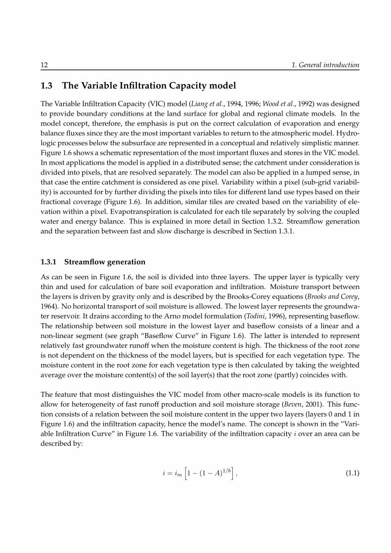
1.3 The Variable Infiltration Capacity model
The Variable Infiltration Capacity (VIC) model (Liang et al., 1994, 1996;Wood et al., 1992) was designed
to provide boundary conditions at the land surface for global and regional climate models. In the
model concept, therefore, the emphasis is put on the correct calculation of evaporation and energy
balance fluxes since they are the most important variables to return to the atmospheric model. Hydro-
logic processes below the subsurface are represented in a conceptual and relatively simplistic manner.
Figure 1.6 shows a schematic representation of themost important fluxes and stores in the VICmodel.
In most applications the model is applied in a distributed sense; the catchment under consideration is
divided into pixels, that are resolved separately. The model can also be applied in a lumped sense, in
that case the entire catchment is considered as one pixel. Variability within a pixel (sub-grid variabil-
ity) is accounted for by further dividing the pixels into tiles for different land use types based on their
fractional coverage (Figure 1.6). In addition, similar tiles are created based on the variability of ele-
vation within a pixel. Evapotranspiration is calculated for each tile separately by solving the coupled
water and energy balance. This is explained in more detail in Section 1.3.2. Streamflow generation
and the separation between fast and slow discharge is described in Section 1.3.1.
1.3.1 Streamflow generation
As can be seen in Figure 1.6, the soil is divided into three layers. The upper layer is typically very
thin and used for calculation of bare soil evaporation and infiltration. Moisture transport between
the layers is driven by gravity only and is described by the Brooks-Corey equations (Brooks and Corey,
1964). No horizontal transport of soil moisture is allowed. The lowest layer represents the groundwa-
ter reservoir. It drains according to the Arno model formulation (Todini, 1996), representing baseflow.
The relationship between soil moisture in the lowest layer and baseflow consists of a linear and a
non-linear segment (see graph “Baseflow Curve” in Figure 1.6). The latter is intended to represent
relatively fast groundwater runoff when the moisture content is high. The thickness of the root zone
is not dependent on the thickness of the model layers, but is specified for each vegetation type. The
moisture content in the root zone for each vegetation type is then calculated by taking the weighted
average over the moisture content(s) of the soil layer(s) that the root zone (partly) coincides with.
The feature that most distinguishes the VIC model from other macro-scale models is its function to
allow for heterogeneity of fast runoff production and soil moisture storage (Beven, 2001). This func-
tion consists of a relation between the soil moisture content in the upper two layers (layers 0 and 1 in
Figure 1.6) and the infiltration capacity, hence the model’s name. The concept is shown in the “Vari-
able Infiltration Curve” in Figure 1.6. The variability of the infiltration capacity i over an area can be
described by:
i = im
[
1 − (1 −A)1/b]
, (1.1)

1.3. The Variable Infiltration Capacity model 13
Figure 1.6: Schematic description of hydrological pro-
cesses as they are represented in the VIC-model. Source:
http://www.hydro.washington.edu/Lettenmaier/Models/VIC/VIChome.html.
where i is the infiltration capacity up to which the soil is filled, and im is the maximum infiltration
capacity of the soil, which depends on the soil moisture storage capacityWmax by im = (1 + b)Wmax.
A represents the fraction of the grid cell that has an infiltration capacity less than i and is derived from
the soil moisture contents in the upper layersW by:
A = 1 −(
1 − W
Wmax
)b/(1+b)
, (1.2)
Equation 1.1 basically describes the dynamics of runoff contributing areas as a function of the mean
soil water content (Lohmann et al., 1998a). The shape parameter b is thus a measure for the amount
of variability in topography within a grid cell. For b = 1 therefore, the distribution is uniform and
there is no heterogeneity present in streamflow generation. In Figure 1.6, As is that fraction of the grid
cell area that is saturated at the beginning of the time step, corresponding with initial soil moisture
depthW0. For a precipitation amount P , the amount of water that infiltrates is the areally integrated
infiltration capacity∫ i0+Pi0
A(i)di, indicated as ∆W in Figure 1.6. The remainder P −∫ i0+Pi0
A(i)di,

14 1. General introduction
indicated as Qd, contributes to surface runoff (Wood et al., 1992).
1.3.2 Evapotranspiration
VIC solves the coupled energy and water balance to calculate the actual evapotranspiration and the
associated turbulent fluxes, i.e. the calculation of evapotranspiration (and the latent heat flux) is iter-
ated until the energy balance closes:
Rnet = λE +H +G, (1.3)
whereRnet is the net radiation, λ is the latent heat of vaporization ofwater,E is the evapotranspiration
flux, H is the sensible heat flux and G is the ground heat flux. Rnet, λE, H and G all depend on the
surface temperature Ts. As an initial guess, Ts is set equal to the air temperature. All energy fluxes
are calculated using this initial temperature. λE is the connection to the water balance, therefore its
calculation is explained in more detail. First, potential evaporationEp is calculated using the Penman-
Monteith equation (Penman, 1948; Monteith, 1965):
λEp =∆Rnet + ρacp
[es(z)−e(z)]ra
∆ + γ(
1 + rc
ra
) , (1.4)
where es(z) and e(z) are the saturated and actual vapor pressure at height z (the height where the
wind speed is measured) respectively, ∆ is the rate of change of es with temperature, ρa and cp are
respectively the density and specific heat capacity of air, γ is the psychrometric constant, ra is the
aerodynamic resistance and rc is the canopy resistance. ra depends on vegetation properties such as
surface roughness and trunk height. For the equations to calculate ra,H , andG, see for example Liang
et al. (1994).
From Ep and the contents of the upper soil moisture layer an actual evaporation Ea is calculated,
according to:
Ea = Ep
(
∫ As
0dA+
∫ 1
As
i0
im[
1 − (1 −A)1/b]dA
)
, (1.5)
Note that in Equation 1.5, the area is divided in a saturated part, which evaporates at the potential
rate, and an unsaturated part, which evaporates at a rate that is reduced by the storage deficit. Equa-
tion 1.5 provides a new λE and the energy balance is solved again, yielding updated energy fluxes
and Ts. Except for the bare soil evaporation described by Equation 1.5, transpiration and canopy in-
terception evaporation are calculated. If the surface is vegetated, vegetation is divided in a wet and
a dry fraction: from the wet fraction canopy evaporation occurs (rc = 0) and from the dry fraction

1.4. Problem description and thesis outline 15
transpiration occurs.
1.3.3 Streamflow routing
The sum of surface runoff and baseflow from each grid cell is routed to the basin outlet (or any other
user defined location in the river basin) using an algorithm developed by Lohmann et al. (1996). The
algorithm is used “stand-alone”, i.e., output of the VIC model is post-processed to obtain streamflow.
Therefore, no river bed infiltration or feedbacks due to flooding are taken into account. The concept
is shown in the right panel of Figure 1.6. Based on digital elevation data, the river basin is divided in
grid cells at the same spatial resolution as the VIC model, each with an average elevation. Each grid
cell then drains to its lowest neighbour. It is assumed that each grid cell drains directly in the channel
network. River routing is then carried out with the linearized St.Venant equation:
δQ
δt= D
δ2Q
δx2− C
δQ
δx, (1.6)
where D and C are diffusivity and celerity respectively. Equation 1.6 can be solved by convolution
integrals:
Q(x, t) =
∫ t
0U(t− s)h(x, s)ds, (1.7)
where U is the sum of surface runoff and baseflow from the VIC model, and h(x, s) is the impulse
response function of Equation 1.6 (Lohmann et al., 1996, 1998a):
h(x, t) =x
2t√πtD
exp
(−(Ct− x)2
4Dt
)
, (1.8)
where x is the total channel length running through a grid cell.
1.4 Problem description and thesis outline
In the first part of this thesis, Chapters 2, 3 and 4, the VIC model and the Rhine river basin will play
a central role. In Chapter 2, the VIC model is first applied to the Rhine basin, and compared to a
more simple and conceptual water balance model. The latter model is representative for models that
have been used in climate change impact assessments before (e.g. Middelkoop et al., 2001; Kwadijk and
Middelkoop, 1994; Shabalova et al., 2003; Lenderink et al., 2007). The VIC model has several advantages
compared to these models. First, evapotranspiration is calculated in a more physically based manner
(see Section 1.3.2), whereas in the more simple water balance models it is often based on temperature
only. Second, small-scale heterogeneity in land use, elevation and topography is taken into account

16 1. General introduction
in the VIC model, whereas it is not in simpler water balance models. Third, water balance models use
precipitation and temperature as input, while the VIC model can employ additional climate model
output where this is available, such as radiation, humidity and wind speed. Water balance models
thus rely very much on calibrated parameter values to reproduce historical streamflow. The physical
basis behind these parameters is often limited, and it is highly questionable whether the values for
these parameters remain stable under changing climate conditions. Although the VIC model also
relies on model calibration of certain parameters, they are more physically based, thus reducing the
sensitivity to calibrated parameter values.
Another advantage of the physical basis of the calculation of evapotranspiration for different vege-
tation types, is the possibility to evaluate scenarios of land use change. This is done in Chapter 3.
Land use change can have significant effects on rainfall-runoff processes. For example, research in-
dicated that deforestation can amplify flood risk (e.g. Laurance, 2007; Bradshaw et al., 2007) through
decreasing infiltration capacity, transpiration and interception (Clark, 1987). Urbanization decreases
the infiltration capacity and transpiration as well through the removal of vegetation and the creation
of impervious surfaces (e.g. Dow and DeWalle, 2000; DeWalle et al., 2000). In the Eururalis project (Ver-
burg et al., 2006a), four land use change scenarios for Europe were developed, which are based on
the story lines described by the SRES scenario families (Section 1.1.3). Based on socio-economic and
demographic developments, and a model that allocates resulting land use types to individual pixels
(Verburg et al., 2008), four high-resolution (1 km2) land use scenarios for the year 2030 were obtained.
These scenarios, as well as two hypothetical scenarios in which all agricultural land in the Rhine basin
is replaced by either forest or grassland, are evaluated in terms of streamflow using the VIC model.
Climate conditions are kept constant for all land use scenarios.
In Chapter 4, the land cover is kept constant and the influence of climate change is investigated. To
this end, three climate scenarios are used to force the VIC model. All scenarios consist of model out-
put from a GCM, downscaled using an RCM. Each scenario is based on one of three SRES-emission
scenarios (A2, A1B and B1; see Section 1.1.3). Compared to previous studies, the spatial resolution of
the climate scenarios that are employed here is relatively high (∼ 10 km), whereas resolutions of 25 or
50 km were typically used in other studies (e.g. Shabalova et al., 2003; Lenderink et al., 2007). This high
resolution enables precipitation events that typically cause extreme peak flows to be simulated more
accurately, because such events are often convective in nature and their spatial extent is relatively
small. There are many uncertainties involved in such a climate change impact assessment: even in
the reproduction of the current climate, there is a large range of model outcomes, both from GCMs
and RCMs (Covey et al., 2003; Jacob et al., 2007). Apart from that, there is uncertainty involved in the
hydrological model and its parameterization, and in the GCM forcings (emission scenarios). In Chap-
ter 4, three plausible climate scenarios are analyzed in terms of their effects on average and extreme
streamflow (both peak flows and low flows), while the uncertainties involved are acknowledged and
discussed.

1.4. Problem description and thesis outline 17
As was mentioned in Section 1.1.2, in the Colorado River Basin (CRB) low-frequency (interannual to
interdecadal) climate variability has an important influence on the hydrologic system. It thus presents
an excellent study area to investigate and quantify this influence, which is done in Chapter 5. The CRB
recently experienced a severe multi-year drought (Seager et al., 2007). Water availability is an impor-
tant issue in the Colorado basin: population grows explosively, while climate models predict severely
dry conditions (Barnett and Pierce, 2008; Cook et al., 2004). Previously, precipitation and streamflow in
the CRB have been linked to ENSO (e.g.Canon et al., 2007;Hidalgo and Dracup, 2003) and PDO (e.g.Ger-
shunov and Barnett, 1998). Total terrestrial water storage (TWS) has received relatively little attention.
It is, however, an important variable because it integrates hydrological processes in the catchment,
such as snow accumulation, evapotranspiration and recharge. Different approaches exist to estimate
TWS, several of which have been compared by Troch et al. (2007). In the latter study, storage dynamics
as simulated by VIC proved to be similar to that of other methods. In Chapter 5, anomalies of TWS
and its components as they are simulated by VIC are used to investigate the effects of low-frequency
cycles of Pacific ocean temperature on the hydrology of the Colorado basin.
As was described in Section 1.3, the representation of subsurface hydrological processes in the VIC
model is relatively simplistic compared to the representation of land-atmosphere interactions (evapo-
transpiration and vegetation). At a large spatial scale, such as that of the Rhine basin, it is not possible
to explicitly model all existing heterogeneity in topography, vegetation and soil. It, therefore, needs to
be parameterized. Chapter 6 focusses on different approaches to do this. The area of interest is a small
Alpine sub-catchment of the Rhine basin: the Rietholzbach in Switzerland. Three approaches to pa-
rameterize small-scale variability of topography are investigated: (1) the statistical approach of VIC,
described in Section 1.3.1; (2) the TOPMODEL approach (Beven and Kirkby, 1979; Famiglietti and Wood,
1994), in which from a high-resolution digital elevation model areas of hydrologically similar behav-
ior are identified; and (3) the hillslope approach, in which the hydrological behavior of a hillslope
is modeled and upscaled to a larger spatial scale using hillslope similarity parameters. Streamflow
and spatially averaged evapotranspiration resulting from all model approaches are compared to each
other and to observed values.
In Chapter 7, finally, the most important conclusions from this thesis are summarized and possible
directions for further research are discussed.


Chapter 2
Water balance versus land surface model in the simulation of Rhine riverdischarges
This chapter is a modified version of: R. T. W. L. Hurkmans, H. de Moel, J. C. J. H. Aerts and P. A. Troch (2008),
“Water balance versus land surface model in the simulation of Rhine river discharges,”, Water Resour. Res., 44,
W01418, doi:10.1029/2007WR006168

20 2. Water balance versus land surface model in the simulation of Rhine river discharges
Abstract
Accurate streamflow simulations in large river basins are crucial to predict timing and magnitude of floods
and droughts and to assess the hydrological impacts of climate change. Water balance models have been
used frequently for these purposes. Compared to water balance models, however, land surface models carry
the potential to more accurately estimate hydrological partitioning and thus streamflow, because they solve
the coupled water and energy balance and are able to exploit a larger part of the information provided by
regional climate model output than water balance models. Due to increased model complexity, however, they
are also more difficult to parameterize. The purpose of this study is to investigate and compare the accuracy
of streamflow simulations of a water balance approach (STREAM) and a land surface model (VIC) approach.
Both models are applied to the Rhine river basin using regional climate model output as atmospheric forcing,
and evaluated using observed streamflow and lysimeter data. We find that VIC is more robust and less
dependent on model calibration. Although STREAM performs better during the calibration period (Nash-
Sutcliffe efficiency (E) of 0.47 versus E = 0.29 for VIC), VIC more accurately simulates discharge during
the validation period, including peak flows (E = 0.31 versus E = 0.21 for STREAM). This is the case for
most locations throughout the basin, except for the Alpine part where both models have difficulties due to the
complex terrain and surface reservoirs. In addition, the annual evaporation cycle at the lysimeters is more
realistically simulated by VIC.

2.1. Introduction 21
2.1 Introduction
River discharge integrates hydrological processes at the catchment scale and can bemeasured directly,
as opposed to many other catchment fluxes (e.g., evaporation, precipitation). Streamflow is thus a
suitable variable to validate and/or compare hydrological model performances. In Central Europe,
recent floods in the Rhine (1993 and 1995), Elbe (2002) and Danube (2002), as well as droughts (e.g.,
the summer of 2003) caused billions of euros of damage (Kleinn et al., 2005). Improving streamflow
simulations in these densely populated large river basins is important to accurately predict timing and
magnitude of floods and droughts (Nijssen et al., 1997). Climate change is believed to affect streamflow
characteristics mainly because of two reasons: first, the warming-related shift from snow to rainfall
will change the seasonal streamflow cycle in rivers which have their source region in the Alps (includ-
ing the Rhine). Second, there is increasing evidence for an acceleration of the hydrological cycle and
an associated increase in precipitation intensity during winter (Kleinn et al., 2005). Numerous studies
have been carried out to quantify the impact of climate change on extreme value distributions of river
streamflow, indicating a projected increase in extreme winter floods and more droughts in summer
(Middelkoop et al., 2001; Milly et al., 2005; Aerts et al., 2006; de Wit et al., 2007; Kwadijk, 1993; Buishand
and Lenderink, 2004). In these studies, future climate data were obtained from climate models, down-
scaled either using statistical weather generators (Beersma et al., 2001; Eberle et al., 2002; Dibike and
Coulibaly, 2005), or regional climate models (RCMs) (e.g., Christensen et al., 2004; Kleinn et al., 2005).
Although the latter have the advantage to supply a sufficient number of meteorological variables at
a high enough spatial and temporal resolution to force more sophisticated models, often conceptual
water balance models have been used to simulate future streamflow. Examples of water balance mod-
els for the Rhine include HBV (Hydrologiska Byrans Vattenbalansavdelning; (Bergstrom and Forsman,
1973; Lindstrom et al., 1997)), Rhineflow (Kwadijk, 1993) and STREAM (Spatial Tools for River basins
and Environment and Analysis of Management options; (Aerts et al., 1999, 2006)).
To accurately simulate streamflow, it is essential to have a realistic description of all relevant land
surface processes, including the partitioning of available energy. Errors in estimates of evaporation
propagate into similar errors in other terms of the energy and water balance and ultimately affect
streamflow prediction (Koster et al., 2000). Water balance models typically use empirical or statis-
tical methods to estimate potential evaporation based on temperature. For example, Rhineflow and
STREAMuse an approach developed by Thornthwaite andMather (1957) that is based on daily temper-
ature measurements. Present day land surface models (LSMs) on the other hand, derive evapotran-
spiration from coupled water and energy balance simulations (Liang et al., 1994; Famiglietti and Wood,
1994), and are able to utilize additional information provided by RCM output, such as solar radiation,
wind speed, specific humidity and atmospheric pressure. Therefore, LSMs carry the potential to more
accurately estimate hydrological partitioning (evaporation, soil moisture, surface runoff and stream-
flow). Because of the complex model structure and the large number of parameters in LSMs, they
are generally more difficult to parameterize. LSM intercomparison experiments have demonstrated
large variability in simulated land surface-atmosphere fluxes and streamflow using different LSMs

22 2. Water balance versus land surface model in the simulation of Rhine river discharges
(e.g., Pitman et al., 1999; Wood et al., 1998; Lohmann et al., 2004). The original purpose of LSMs was to
represent the land surface in (regional) climate simulations used for climate models and numerical
weather prediction (e.g., Liang et al., 1994; Koster et al., 2000; Zeng et al., 2002; Dai et al., 2003). Recently,
LSMs have been used for (experimental) streamflow forecasting as well (e.g.,Wood et al., 2005). How-
ever, many studies assessing climate change impacts use water balance models, as well as short-term
flood forecasting systems (e.g., in The Netherlands, Sprokkereef , 2001a).
To our knowledge, no direct comparison between a water balance model and a LSM in such applica-
tion has yet been carried out. The purpose of this study is to investigate and compare the accuracy of
streamflow simulations of a water balance approach and a more detailed land surface modeling ap-
proach, including the energy balance. We use a state of the art LSM (the Variable Infiltration Capacity
(VIC) model, version 4.0.5) and a water balance model (STREAM) to simulate hydrological partition-
ing in the Rhine river basin. STREAM is a distributed water balance model that has been adapted to
simulate streamflow at the basin outlet. Previous applications of VIC to a range of catchment scales
have used streamflow indicators for verifying simulations and have demonstrated satisfactory results
(Nijssen et al., 1997, 2001; Lohmann et al., 1998b). In addition to solving the coupled water and energy
balance, we applied VIC in the water balance mode (VIC-WB): instead of obtaining surface tempera-
ture by solving the energy balance, it is assumed equal to air temperature, thereby avoiding iterative
solution of the energy balance. VIC-WB is an intermediate between VIC and STREAM in that it does
not solve the coupled water and energy balance but does account for, for example, sub-grid variabil-
ity. In this way the influence of solving the energy balance is separated from that of other differences
in the formulation of the models, such as the sub-grid variability parameterization in VIC (see Sec-
tion 2.3), and investigated more specifically. All models are calibrated to a similar extent (as is further
explained in Section 2.4) and subsequently applied to the Rhine basin in the period between 1993 and
2003 using RCM output as meteorological forcing (Jacob, 2001). Within this period, the Rhine basin
experienced the near-floods in 1993 and 1995, as well as a severe low flow period during the summer
of 2003. We compare model simulations for these extreme flows. To evaluate streamflow simulations
from all three models, we use observed streamflow data from main tributaries, as well as data from
several locations along the main Rhine branch. In addition, lysimeter data is employed to evaluate
the simulation of evaporation at specific locations within the basin.
2.2 Study area and data
The river Rhine originates in the Swiss Alps and drains large parts of Switzerland, Germany and The
Netherlands. After crossing the German-Dutch border near Lobith, the river splits into three distribu-
taries before discharging in the North sea. Therefore, only the area upstream of Lobith is considered
here, which measures about 185,000 km2. Streamflow gauges at the mouths of five major tributaries
(Lahn, Mosel, Main, Neckar and Ruhr) and at three locations along the main branch (Maxau, Ander-
nach and Lobith) were used to compare the models. The Rhine basin is described in more detail in

2.2. Study area and data 23
Figure 2.1: Location of Rhine basin and streamflow gauges (left) and the dis-
cretization of the basin for routing purposes (right). In the left plot, also lysimeter
locations are shown.
Section 1.2, and in Table 1.1 streamflow gauges and main streamflow characteristics of the main Rhine
tributaries are listed. The Rhine basin and the location of the gauging stations are shown in Figure 2.1.
All three models are forced using downscaled ECMWF ERA15 reanalysis data
(http://www.ecmwf.int/research/era/), provided by theMax Planck Institut furMeteorologie, Ham-
burg, Germany (MPI). Downscaling was carried out at MPI using the regional climate model REMO
(Jacob, 2001). This dataset will be referred to as ERA15d hereafter. The dataset comprises the years
1993 through 2003, with data available every three hours at a spatial resolution of 0.088 degrees (about
9 km). In Figure 2.2 monthly climatologies of the seven variables that were used to force VIC and
VIC-WB, i.e., precipitation, temperature, specific humidity, surface pressure, incoming longwave and
shortwave radiation and windspeed, are shown. To compare this data to observations, an additional
meteorological dataset is used from the International Commission for the Hydrology of the Rhine
basin (CHR), referred to as CHR hereafter. This dataset contains daily values of precipitation and
temperature and is based on observations from 36 stations throughout the basin (Sprokkereef , 2001b).
Temperature and precipitation for the years present in both datasets (1993 through 1995) are com-
pared. In Figures 2.3 and 2.4, the results are shown. Monthly values of precipitation match reason-
ably well (R2 = 0.73), however at daily and weekly scales, correlations are very low. Temperatures are
structurally about 1.5◦C higher for ERA15d (Figures 2.2 and 2.4). This difference is occurring through-
out the basin, but it is smallest in the relatively flat areas. In summer, the difference is maximal (about
2◦C). Precipitation differs greatly between both datasets during winter (DJF) in the Alpine area, in
some areas up to 200 mm, probably due to significant amounts of snow that are not measured by
the observation network used in the CHR dataset. In summer, differences in precipitation are small.

24 2. Water balance versus land surface model in the simulation of Rhine river discharges
5101520
[mm
/day
]
Precipitation
12345
Pre
cipi
tatio
n Avg. ERA15d: 937 mmAvg. CHR: 1082 mm
−10−5
05
1015202530 Avg. ERA15d: 10.45 °C
Avg. CHR: 8.81 °C
Tem
p. [°
C]
Temperature
0.005
0.010
0.015 Avg. 0.0072 kg/kg
Hum
idity
[kgk
g−1 ]
Specific humidity
0.99
1
1.01
1.02
1.03
1.04
Avg. 101641 PaP
ress
ure
[Pa]
Pressure
J F M A M J J A S O N D0
50100150200250300350400450
Rad
iatio
n [W
m−
2 ]
Downward radiation
Avg. SW: 135.0 W/m2; LW: 310.7 W/m2
Shortwave Longwave
J F M A M J J A S O N D123456789
Avg. 3.35 m/sW
ind
spee
d [m
s−1 ]
Windspeed
Figure 2.2: Monthly averages (solid), maxima and minima (dash-dotted) of forc-
ing variables in the ERA15d dataset. For precipitation (top left) and temperature
(top right) also the CHR dataset is shown. Also annual averages (sums for pre-
cipitation) are shown. Note that for the CHR dataset, only 3 years of data are
used because only three years were overlapping in the datasets.
It is clear that both datasets have their shortcomings. However, in the remainder of this paper we
use the ERA15d because a) CHR does not contain all input fields to run VIC, b) only three years of
overlapping data (i.e., 1993-1995) are available and c) the re-analysis data is similar to RCM output
that is generally used to assess the hydrological impacts of climate change.
For land use, the Pan-European Land Cover Monitoring and Mapping-database (Mucher et al., 2000)
was used. Soil data were taken from the global FAO dataset (Reynolds et al., 2000). Lysimeter data
were available for two stations located in very different parts of the basin. Rheindahlen (51.16N,
6.33, elevation about 75 m.a.s.l.) is close to the basin outlet and Rietholzbach (47.38N, 8.99, eleva-
tion about 700 m.a.s.l.) is located in the Alpine part of the basin (Figure 2.1). At both lysimeter
sites, the dominant vegetation type is grass. More information about the lysimeter station at Rhein-
dahlen can be found in Xu and Chen (2005). Of the four available lysimeters at Rheindahlen, we used

2.3. Description of models 25
0 2 4 6 8 10 12 14 16 180
2
4
6
8
10
12
14
16
18R2 daily: 0.42R2 weekly: 0.63R2 monthly: 0.73R2 seasonally: 0.74
CHR [mm day−1]
ER
A15
d [m
m d
ay−
1 ]
1:1
Figure 2.3: ERA15d versus CHR precipitation. The period 1993-1995 was used
for the comparison. Average precipitation amounts of both datasets are plotted
against each other, aggregated over 1, 7, 30 and 90 days. For every aggregation
period, the resulting square of the correlation coefficient (R2) is displayed in the
upper left corner.
lysimeter nr. 3, in accordance with Xu and Chen (2005). The lysimeter at Rietholzbach is described at
http://www.iac.ethz.ch/research/rietholzbach/instruments/.
2.3 Description of models
STREAM (Spatial Tools for River basins and Environment and Analysis of Management options), is
a distributed, grid based water-balance model (Aerts et al., 1999, 2006), based on the Rhineflow ap-
proach (Kwadijk, 1993). The water balance is solved for every grid cell in the basin at a daily timestep.
The model consists of three storage reservoirs: snow storage, soil moisture storage and groundwater
storage, dividing outflow into a fast and a slow component. The fast component is affected by soil
moisture storage and the slow component by ground water storage, both behaving as linear reser-
voirs. Potential evapotranspiration is derived from surface temperature, following the approach of
Thornthwaite and Mather (1957). Actual evapotranspiration is calculated using the soil moisture stor-
age and the so-called ’accumulated potential water loss’, see Thornthwaite and Mather (1957). Snow
accumulation is equal to precipitation when temperature is below zero degrees Celsius, snow melt
linearly depends on temperature. Both fast and slow flow are routed to the basin outlet by flow ac-

26 2. Water balance versus land surface model in the simulation of Rhine river discharges
Figure 2.4: Spatial patterns of temperature and precipitation from the CHR and
ERA15d datasets. The upper four maps show temperature, the lower four maps
precipitation. In the right four maps, annual mean temperature and annual cu-
mulative precipitation are plotted. In the left four maps, average differences be-
tween the datasets are shown for two seasons: winter (DJF) and summer (JJA).
Positive values indicate an overestimation of ERA15d, with respect to CHR. Av-
erages are computed from the years 1993 through 1995.
cumulation under the assumption of a constant flow velocity. An overview of parameters typically
used for calibration is given in Section 2.4. Because STREAM only needs precipitation and temper-
ature as dynamic input variables, its application is relatively simple. STREAM has been applied to
various river basins, including the Krishna river in India (Bouwer et al., 2006) and many of the major
catchments in the world in a study on Holocene and future discharges (Aerts et al., 2006; Ward et al.,
2007).
The Variable Infiltration Capacity (VIC) model (Liang et al., 1994, 1996; Liang and Xie, 2001), is a
variable-layer soil-vegetation-atmosphere transfer (SVAT) scheme for general and regional circula-
tion and weather prediction models. Its most distinguishing aspect in comparison with other LSM is
its variable infiltration capacity curve, which is described by:

2.3. Description of models 27
Figure 2.5: Relationship between soil moisture content in the lowest layerWc and
base flow D. Dm represents maximum base flow velocity, Ds is a fraction of Dm
and Ws is a fraction of Wc. The point (Ws,Ds) represents the point where the
curve becomes nonlinear.
I = Im
[
1 − (1 −A)1/β]
(2.1)
where I and Im are the infiltration capacity and maximum infiltration capacity, respectively. A is
the fraction of an area for which the infiltration capacity is less than I and β is a shape parameter.
Drainage from the upper to the lower layers is assumed to be driven by gravity only, using the Brooks
and Corey (1964) relationship to estimate hydraulic conductivity. Baseflow is modeled following the
ARNO model formulation (Todini, 1996). The relation between soil moisture in the lowest layer and
base flow is shown in Figure 2.5. These concepts, as well as the calculation of evapotranspiration is
described in more detail in Section 1.3 and shown in Figure 1.6. The parameters in Figure 2.5 and β, as
well as depths of the soil layers, are typically used for model calibration (e.g., Lohmann et al., 1998a).
See Section 2.4 for more details about model calibration. When snow is present on the ground, the
model is coupled with a two layer energy- and mass-balance model. Snow can also be intercepted by
the canopy, melt from the canopy snowpack is simulated using a simplified energy balance model.
More details about the VIC model can be found in Section 1.3. The VIC model can operate in two
modes: in the energy balance mode, the energy balance is solved iteratively to obtain the surface tem-
perature, whereas in the water balance mode, surface temperature is assumed equal to air tempera-
ture. In both modes, potential evapotranspiration is calculated using the Penman-Monteith equation.
In the energy balance mode, a time step of 3 hours is used, in correspondence with availability of
forcing data, whereas in water balance mode the model is integrated at a daily time step. Therefore
simulation times are drastically reduced compared to the full mode.
Routing of surface runoff and base flow from all models is done by the algorithm developed by
Lohmann et al. (1996), which has been applied in combination with VIC by Lohmann et al. (1998a,b).
The sum of base flow and runoff from the models is convoluted with a normalized impulse response

28 2. Water balance versus land surface model in the simulation of Rhine river discharges
function, based on the linearized St. Venant equation (e.g., Troch et al., 1994), assuming that water
from each grid cell flows into the channel in the steepest direction to one of its eight neighbors.
2.4 Model calibration
All three models were calibrated using daily observed streamflow at Lobith for the year 1993. Only
one year was used to limit the amount of calibration time. Because 1993 contains a relatively dry
summer, as well as a near flood event, it was considered representative for the total period. Because
no data were available before 1993 and, based on preceding streamflow observations, conditions and
model storages in October 1993 were assumed to be similar to January 1993, the model states (i.e.,
moisture contents, snow pack) of October 1993 were used to initialize all model simulations in Jan-
uary 1993. STREAM was calibrated using a built-in optimization routine, iteratively changing the
parameters one-at-a-time and minimizing the mean absolute difference between observed and simu-
lated streamflow, and then fine-tunedmanually. Four parameterswere optimized following e.g.,Aerts
et al. (2006): a factor C to adjust the land use dependent crop factor that defines potential evapotran-
spiration for different land use types, a depletion factorD for the groundwater reservoir, a factorX to
separate between direct runoff and groundwater recharge, and finally a parameterH that defines the
relation between temperature and reference evapotranspiration. To calibrate VIC, seven parameters
influencing the shape of the hydrograph and the total outflow volume were subjected to a sensitivity
analysis. Based on this analysis, the depth of the (very thin) upper layer and the baseflow parameter
Ws (see Figure 2.5) appeared to have no influence on the resulting hydrograph and were therefore left
out of the calibration procedure to save computation time. Parameters influencing potential evapo-
transpiration, differing per vegetation type, were left at their default values. The resulting parameters
for optimization are, similar to former applications (Lohmann et al., 1998a; Liang et al., 1994): Dm and
Ds to define the relation between baseflow and soil moisture in the lowest layer (see Figure 2.5), the
shape parameter β in Eq. 2.1 and the depths of the lower two layers d2 and d3. Because these pa-
rameters are not transferable between the full and energy modes, VIC was re-calibrated for the water
balance mode, using the same parameters. For optimizing the objective function O a power transfor-
mation was used to balance sensitivity to peak flows and low flows. The objective function can be
written as:
O =1
N
N∑
i=1
(
Qλobs,i −Qλ
sim,i
)
λ(2.2)
whereN is the number of time steps andQobs andQsim are observed and simulated discharge respec-
tively. Both are raised to the power λwhich is taken as 0.3 in this study because this gives an optimal
balance between sensitivity to peak and low flows (Misirli et al., 2003).

2.4. Model calibration 29
To calibrate the models to a comparable level, all parameters were kept uniform in space. To enable
streamflow comparison at other streamflow gauges than Lobith only, STREAM surface runoff and
base flow were routed using the VIC routing algorithm. Figure 2.6 shows daily streamflow in 1993
for VIC (both modes) and STREAM compared to observations. For STREAM, two hydrographs are
plotted: one obtained by routing using the original STREAM routing scheme (STREAM1) and one ob-
tained by routing using the VIC algorithm (STREAM2). The VIC routing algorithm tends to slightly
delay runoff peaks compared to the original STREAM routing scheme. Varying celerity and diffusiv-
ity in the VIC routing algorithm did not change this behavior. To remove the influence of the routing
algorithm that was used, hereafter 10-daily averaged streamflow values are evaluated at gauging sta-
tions other than Lobith. For analyses at the Lobith gauging station that require daily streamflow (such
as peak flow analyses), daily discharge obtained by the original STREAM routing algorithm is used
for the STREAM simulations.
In Table 2.1, correlation coefficients (ρ), Nash-Sutcliffe modeling efficiencies ((E; Nash and Sutcliffe,
1970) and relative volume errors (RVE) for both the calibration and validation period are shown for
daily discharge at Lobith. During the calibration period, STREAM performs better: E = 0.47 for
STREAM, whereas E = 0.29 for VIC. Also ρ for STREAM is higher (0.77) than for VIC (0.67). As men-
tioned before and can be seen in Table 2.2, routing STREAM output with the VIC algorithm reduces
STREAM’s performance drastically for daily discharge. The performance of VIC-WB is in between
VIC and STREAM with E = 0.39 and ρ = 0.71. Changing parameters in STREAM has a more di-
rect effect on the resulting hydrograph, whereas in VIC a more extensive calibration including more
parameters would have been necessary to obtain similar results. For VIC-WB, changing the calibra-
tion parameters has a larger effect compared to VIC yielding better results. The rather poor results in
the calibration period in terms of Nash-Sutcliffe values are partly explained by an overestimation of
streamflow in summer. The inset of Figure 2.6 shows that this was mainly caused by too high precip-
itation in the ERA15d dataset.
To investigate the influence of this biased forcing data, VIC and STREAM were also forced by pre-
cipitation from CHR. The other required forcing variables are from ERA15d, because they were not
available in the CHR dataset. Figure 2.7 shows daily simulated discharges at Lobith for VIC and
STREAM, where precipitation from both ERA15d and CHR is used, for the period 1993 through 1995,
i.e., the periodwhere both forcing datasets overlap. Note that the models were not recalibrated for the
CHR dataset. It appears that both models improve drastically when forced with the CHR precipita-
tion: for VIC, E increases from 0.45 to 0.59, for STREAM from 0.47 to 0.56. The correlation coefficient
on the other hand increases especially for STREAM; from 0.81 to 0.92, whereas for VIC this increase is
much less: from 0.79 to 0.83. In the summer of 1993, VIC with CHR precipitation now simulates dis-
charge very well, while STREAMunderestimates discharge, as was to be expected because the model
was not recalibrated.

30 2. Water balance versus land surface model in the simulation of Rhine river discharges
30 60 90 120 150 180 210 240 270 300 330 3600
2000
4000
6000
8000
10000
12000
14000
DOY in 1993
Dis
char
ge [m
3 s−
1 ]Observed
VIC
VIC−WB
STREAM1
STREAM2
−2
0
2
mm
d−
1 (ERA15d−CHR)
J F M A M J J A S O N D−2
0
2×1
03 m3 s
−1
(VIC/STREAM−Obs)
Figure 2.6: Simulated and observed daily streamflow at Lobith for the calibra-
tion period (1993). VIC-WB represents the VIC simulation in the water balance
mode, STREAM1 represents the results of STREAM internal routing used for cal-
ibration and STREAM2 represents result of STREAM output routed by the VIC
algorithm. The upper panel of the inset shows the difference between ERA15d
and CHR precipitation (positive shows higher ERA15d), the lower panel shows
simulated minus observed monthly discharge for VIC (solid line) and STREAM1
(dash-dotted line).
2.5 Model validation
The calibrated models are evaluated using data from the remaining period, i.e., 1994 to 2003. Ta-
ble 2.2 shows ρ, E and RVE for 10-daily averaged discharge for all streamflow gauges in this period.
During the validation period, VIC (ρ = 0.74, E = 0.31) and VIC-WB (ρ = 0.70, E = 0.40) slightly
improve with respect to the calibration period, whereas ρ (0.63) and E (0.14) for STREAM decrease.
When considering all streamflow gauges, correlation coefficients and most E values are higher for
VIC, although the latter are higher for STREAM at Maxau and Rockenau. For VIC-WB, correlation
coefficients are mostly intermediate. E, however, is often higher for VIC-WB compared to VIC, sug-
gesting a more efficient calibration procedure when VIC is run in water balance mode. For Maxau
and Rockenau, E values for all models are negative. The mountainous nature of these areas, where
complex terrain and snow processes play a larger role than in other parts of the basin, make these ar-
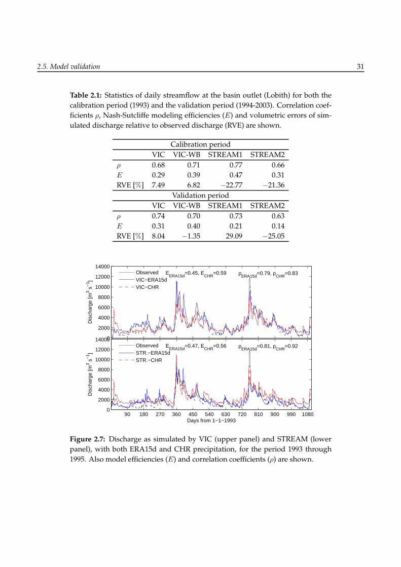
2.5. Model validation 31
Table 2.1: Statistics of daily streamflow at the basin outlet (Lobith) for both the
calibration period (1993) and the validation period (1994-2003). Correlation coef-
ficients ρ, Nash-Sutcliffe modeling efficiencies (E) and volumetric errors of sim-
ulated discharge relative to observed discharge (RVE) are shown.
Calibration period
VIC VIC-WB STREAM1 STREAM2
ρ 0.68 0.71 0.77 0.66
E 0.29 0.39 0.47 0.31
RVE [%] 7.49 6.82 −22.77 −21.36
Validation period
VIC VIC-WB STREAM1 STREAM2
ρ 0.74 0.70 0.73 0.63
E 0.31 0.40 0.21 0.14
RVE [%] 8.04 −1.35 29.09 −25.05
0
2000
4000
6000
8000
10000
12000
14000
Dis
char
ge [m
3 s−
1 ]
EERA15d
=0.45, ECHR
=0.59 ρERA15d
=0.79, ρCHR
=0.83ObservedVIC−ERA15dVIC−CHR
90 180 270 360 450 540 630 720 810 900 990 10800
2000
4000
6000
8000
10000
12000
14000
Days from 1−1−1993
Dis
char
ge [m
3 s−
1 ]
EERA15d
=0.47, ECHR
=0.56 ρERA15d
=0.81, ρCHR
=0.92ObservedSTR.−ERA15dSTR.−CHR
Figure 2.7: Discharge as simulated by VIC (upper panel) and STREAM (lower
panel), with both ERA15d and CHR precipitation, for the period 1993 through
1995. Also model efficiencies (E) and correlation coefficients (ρ) are shown.

32 2. Water balance versus land surface model in the simulation of Rhine river discharges
Table 2.2: Statistics of 10-day streamflow for five tributaries of the Rhine (Lahn,
Main, Mosel, Neckar and Ruhr) and three locations along the main Rhine branch
(Maxau, Andernach and Lobith). For gauge locations, see Figure 2.1. Correlation
coefficients ρ, Nash-Suthcliffe modeling efficiencies (E) and volumetric errors of
simulated discharge relative to observed discharge RVE) are shown for the full
(with energy balance) VIC simulation, the water balance mode simulation (VIC-
WB) and STREAM.
ρ E RVE [%]
VIC VIC-WB STREAM VIC VIC-WB STREAM VIC VIC-WB STREAM
Ruhr 0.74 0.71 0.67 0.52 0.49 0.38 0.80 −7.37 −26.28
Lahn 0.69 0.68 0.62 0.35 0.45 0.19 −35.23 2.06 −47.17
Mosel 0.74 0.78 0.67 0.47 0.53 0.28 −26.67 −19.89 −39.10
Main 0.76 0.75 0.66 0.41 0.27 0.24 −2.88 34.66 −8.00
Neckar 0.73 0.74 0.63 −0.80 −0.33 −0.13 17.89 26.67 −22.13
Maxau 0.70 0.67 0.53 −0.34 −0.02 −0.32 16.42 −5.71 −23.21
Andernach 0.76 0.71 0.63 0.39 0.42 0.03 2.34 −4.58 −27.82
Lobith 0.79 0.75 0.68 0.39 0.49 0.18 8.14 −1.24 −24.87
eas difficult to simulate for all models. It is assumed, however, that applying distributed parameters
in all models would probably significantly improve their performances. From Figure 2.8, it appears
that these are also the areas where peak flows are most severely overestimated by VIC, which is sur-
prising given the topography of the area where layer thicknesses are most likely overestimated by
VIC, because of the uniform layer depths. There are three possible explanations for these overestima-
tions. First, some large surface reservoirs are present in the area, of which Lake Constance (north east
Switzerland, see also Figure 2.1) is the largest with a storage volume of 55 km3. These reservoirs can
have a dampening effect on discharge and are not taken into account in the models. Second, the snow
model in VIC (see Section 2.3) is not calibrated because no snowpack data was available, leading to
a possible overestimation of snow melt. Third, the ERA15d dataset may overestimate precipitation
in the periods corresponding to these peak flows, but no additional precipitation data is available to
verify this. The fact that VIC also overestimates peak flows at other gauges to a lesser degree, which
can be seen in Figure 2.8 for a peak in early 1999, supports this explanation. In the STREAM simula-
tion these peaks are much less distinct (Figure 2.8), which may be explained by the fact that STREAM
is known to slightly underestimate snow melt because at pixels with very high elevations tempera-
ture does not exceed 0◦C, causing snow to constantly accumulate without melting. During low flow
periods, all models underestimate streamflow frequently, although for STREAM this is slightly more
the case than for VIC and VIC-WB.
For Lobith, daily values are analyzed more closely through a peak flow analysis. Because 1993 was a
near flood year in the Rhine basin, both the calibration and validation periods are taken into account

2.5. Model validation 33
0
100
200
300
Dis
char
ge [m
3 s−
1 ] ρ for VIC: 0.81, VIC−WB: 0.76, STREAM: 0.72
Hattingen
0
50
100
150
200
Dis
char
ge [m
3 s−
1 ] ρ for VIC: 0.72, VIC−WB: 0.72, STREAM: 0.65
Kalkofen
0
500
1000
1500
Dis
char
ge [m
3 s−
1 ] ρ for VIC: 0.80, VIC−WB: 0.81, STREAM: 0.69
Cochem
1994 1995 1996 1997 1998 1999 2000 2001 2002 20030
500
1000
1500
Dis
char
ge [m
3 s−
1 ] ρ for VIC: 0.83, VIC−WB: 0.78, STREAM: 0.70
Raunheim
0
200
400
600
800
1000ρ for VIC: 0.80, VIC−WB: 0.79, STREAM: 0.68
Rockenau
0
1000
2000
3000
4000ρ for VIC: 0.74, VIC−WB: 0.70, STREAM: 0.55
Maxau
0
2000
4000
6000ρ for VIC: 0.78, VIC−WB: 0.71, STREAM: 0.64
Andernach
1994 1995 1996 1997 1998 1999 2000 2001 2002 20030
2000
4000
6000
8000ρ for VIC: 0.82, VIC−WB: 0.74, STREAM: 0.69
Lobith
Obs. VIC VIC−WB STREAM
Figure 2.8: Timeseries of monthly discharge as observed, and simulated by VIC,
VIC-WB and STREAM at eight gauges in the Rhine basin. Also monthly correla-
tion coefficients ρ with respect to observations are shown in each plot.
for this analysis. Table 2.3 shows the five highest daily discharges and the five lowest monthly dis-
charges, as observed and simulated at Lobith. In addition, two near-floods (1993 and 1995) and the
extreme low flow period of 2003 are plotted in Figure 2.9. In this Figure, a time window of 20 days
before and after the day of the peaks in 1993 and 1995 is shown. For the low flow period of 2003
the detailed window is 180 days. Also the average discharge during those periods is displayed. The
magnitude of the 1993 event is simulated accurately by VIC with a difference of only 1.5% in the peak
flow, but the peak is delayed by about 2 days, as is the case for nearly all peaks shown in Table 2.3. All
models significantly underestimate the magnitude of the 1995 event, especially STREAM with more
than 40%. Because the 1993 event is the only significant peak in the calibration period, it influenced
the calibration procedure. The accurate simulation of this event is, therefore, not surprising. For the

34 2. Water balance versus land surface model in the simulation of Rhine river discharges
Table 2.3: Peak and low flows at the outlet of the basin (Lobith). The five high-
est daily peaks and the five lowest monthly flows from both the calibration and
validation period are shown. From top to bottom: observed peak discharge, sim-
ulated peak discharge by VIC, VIC-WB and STREAM, relative difference between
simulations and observations for VIC, VIC-WB and STREAM (positive values de-
note higher simulated values), and, only for peak flows, the time lag (τ ) of the
peaks for all models. A positive time lag denotes a delay in the simulation of the
peak.
Peak flows 31-1-95 25-12-93 4-11-98 7-1-03 28-3-01
Max Qobs [m3/s] 11775 11034 9410 9366 8666
∆vic [%] −26.7 1.5 −35.1 −15.5 12.5
∆vic−wb [%] −21.6 11.2 −41.2 −41.4 −13.9
∆stream [%] −44.5 −14.8 −53.2 −55.2 −38.6
τvic [days] 2 2 6 6 4
τvic−wb [days] 1 2 1 3 3
τstream [days] −2 0 −1 4 0
Low flows 9-2003 11-1997 8-1998 9-1996 3-1993
Max Qobs [m3/s] 958 1153 1158 1297 1338
∆vic [%] 38.8 51.4 37.9 6.1 −23.8
∆vic−wb [%] 46.6 4.9 41.0 −6.7 17.8
∆stream [%] 40.7 −10.7 32.8 2.0 −59.0
low flow period in the summer of 2003, all models, especially VIC-WB, overestimate average flow
levels and show more variability than the observations. Because all models show a similar pattern
this is most likely caused by overestimated precipitation events in the forcing data, although in this
period no additional precipitation data is available to verify this possible explanation.
In Figure 2.10 extreme flows are further analyzed through their return periods. A log-Pearson type III
distribution (see Appendix 1) is fitted based on peak discharges to compare and extrapolate extreme
peak flows more easily. To fit the distribution, frequency factors were taken from Table 7.7 in Haan
(1977). Peaks were selected using the Peak-Over-Threshold (POT) approach, where the threshold was
defined as the double of the long-termmean, with the constraint that peaks should be at least 20 days
apart from each other to maintain independency. This resulted in, on average per simulation, just be-
low two peaks per year. Return periods and Pearson fits were based on maximum 10-day discharges
for the eight evaluated streamflow gauges, to remove the influence of streamflow routing, as was
discussed in Section 2.4. For Lobith, the same is shown for maximum daily discharges. As can also
be seen in Figure 2.8, VIC overestimates peak flows especially for Maxau and Rockenau, while for
small tributaries, Kalkofen and Hattingen, all models underestimate them. For the most downstream
gauging stations, Andernach and Lobith, both data and Pearson fits differ strongly for lower return

2.5. Model validation 35
−10 0 +10 days0
2000
4000
6000
8000
10000
12000
Dec 25 1993
Obs: 5525 m3 s−1
VIC: 5578V−WB: 5324STR: 4304
Q [m
3 s−
1 ]
−10 0 +10 days0
2000
4000
6000
8000
10000
12000
January 31 1995
Obs: 5342 m3 s−1
VIC: 5127V−WB: 4050STR: 3325
July August September October November 500
1000
1500
2000
2500
3000
Q [m
3 s−
1 ]
Summer 2003
Obs: 1185, VIC: 1297, V−WB: 1569, STR: 1260 m3 s−1
Obs. VIC VIC−WB STREAM
Figure 2.9: Observed and simulated daily hydrographs at Lobith, zoomed in to
three extreme events in the Rhine basin. The upper panels show the near-floods
of 1993 (left) and 1995 (right), the lower panel shows the low flow period of 2003.
For the peak flows a time window of 20 days before and after the observed maxi-
mum is shown, for the low flow the detailed window is 180 days. The text within
the panels displays the average discharge over the displayed period for all simu-
lations.
times, whereas for high return times (up to 11 years in case of data points), models and observations
agree quite well. For Maxau, however, the range in simulated and fitted discharges keeps increasing
towards higher return times, although for VIC-WB the fit almost coincides with the fit based on ob-
servations for Maxau. However, modeling efficiencies for all models including VIC-WB are negative,
as was mentioned before. Correlations are also relatively low at this gauge: 0.70, 0.67 and 0.53 for
VIC, VIC-WB and STREAM respectively (see Table 2.2). Neither of the models performs very well for
this part of the basin, mainly because of three reasons: first, the terrain is very complex, leading to
local differences in precipitation and radiation that are not taken into account in the models. Second,
although all models account for snow storage and melt to some degree, snow (melt) and glaciers play

36 2. Water balance versus land surface model in the simulation of Rhine river discharges
Table 2.4: Average summer (S), winter (W) and annual (A) totals of precipita-
tion, evaporation, lysimeter (observations) or pixel (models) outflow for the two
lysimeters at Rheindahlen and Rietholzbach. Data from the period 1993-1998 are
used and results from the models VIC, VIC-WB, STREAM are shown.
Rheindahlen Precip. ETP Outflow
S W A S W A S W A
Lysi. 198 198 766 251 85 659 4 112 231
VIC 221 205 851 264 16 541 18 66 242
VIC-WB 221 204 851 209 84 657 24 49 188
STREAM 221 204 849 209 130 686 5 8 37
Rietholzbach Precip. ETP Outflow
S W A S W A S W A
Lysi. 487 386 1578 269 31 541 199 340 1035
VIC 248 160 748 298 6 574 25 43 140
VIC-WB 248 160 748 217 33 509 42 55 230
STREAM 248 160 747 216 78 591 8 8 36
an important role in this area, which further complicates the situation. Third, there are surface wa-
ter reservoirs present in this area that are not accounted for in the models. These surface reservoirs
explain the fact that VIC overestimates peak flows for this area, especially peaks in 1998 and 1999
that are overestimated by VIC originate in the part upstream of Maxau. For gauges near the outlet of
the basin (Lobith and Andernach), STREAM, and to a lesser degree also VIC-WB, underestimate the
relatively low maxima. The fitted lines converge towards higher return periods, however. For these
gauges, VIC simulates the extremes quite well: the fitted lines practically coincide, only for very high
return times the fitted lines slightly diverge.
Figure 2.11 shows monthly evaporation as observed at the two lysimeters at Rheindahlen and Ri-
etholzbach and simulated by VIC and STREAM. VIC accurately mimics the annual cycle at both
lysimeters, hence the high correlations compared to STREAM: 0.97 and 0.80 vs. 0.71 and 0.42 for
Rietholzbach and Rheindahlen respectively. Again, VIC-WB performs intermediate with 0.63 (Rhein-
dahlen) and 0.83 (Rietholzbach). VIC simulates summer evaporation quite well for both locations, but
underestimates winter evaporation, especially for Rheindahlen. For STREAM, modeled evaporation
shows more variability and in winter evaporation is mostly overestimated. VIC-WB also shows more
variability but simulates average winter evaporation very well at both lysimeters (Table 2.4). Both
STREAM and VIC-WB underestimate summer evaporation. The smaller amplitude in evaporation
cycle for VIC-WB and STREAM can be explained by the fact both models assume the surface temper-
ature to be equal to the air temperature, while VIC computes the surface temperature from the energy
balance. In summer, the surface is warmer than the air (giving higher evaporation then when air tem-
perature is used) while in winter the opposite is true. This difference is captured by VIC but neglected

2.5. Model validation 37
50100200
5001000
HattingenQ [m
3 s−
1 ]
50100200
5001000
Kalkofen Q [m
3 s−
1 ]
200
50010002000
5000
Cochem Q [m
3 s−
1 ]
10 100200
50010002000
5000
Raunheim Q [m
3 s−
1 ]
Return period [years]
200
500
1000
2000
Rockenau
2000
5000
8000
Maxau
3000
5000
1000013000
Andernach
10 1003000
5000
1000013000
Lobith
Return period [years]
10 1002000
3500
5000
7500
10000
15000
Return period [years]
Q [m
3 s−
1 ]
Lobith, daily
ObservedVIC VIC−WB STREAM
Figure 2.10: Peak flows selected using a peak-over-threshold approach and their
return periods, as well as a log-Pearson type III distribution fitted through the
data points. The upper eight panels show the fits at the eight evaluated stream-
flow gauges, where STREAM is routed using the VIC routing algorithm, based
on annual maximum 10-day discharges. The lower, larger panel shows the same
only for Lobith, based on annual maximum daily flows, where STREAM is routed
using the original STREAM algorithm.

38 2. Water balance versus land surface model in the simulation of Rhine river discharges
1993 1994 1995 1996 1997 19980
50
100
150
Eva
pora
tion
[mm
]
Rheindahlen
ρ for VIC: 0.80, VIC−WB: 0.63, STREAM: 0.42
1993 1994 1995 1996 1997 19980
50
100
150Rietholzbach
ρ for VIC: 0.97, VIC−WB: 0.83, STREAM: 0.64
Eva
pora
tion
[mm
]
Lysi. VIC VIC−WB STREAM
Figure 2.11: Monthly evaporation for lysimeters Rheindahlen (upper panel) and
Rietholzbach (lower panel) as observed by lysimeters and modeled by VIC, VIC-
WB and STREAM. Correlation coefficients are displayed in the left upper corners.
by VIC-WB and STREAM. When total annual evaporation is considered, VIC simulated evaporation
in Rheindahlen is too low, mainly due to the underestimation in winter, while evaporation simulated
by STREAMand VIC-WB is comparable to observations. VIC’s underestimation in winter may partly
be explained by vegetation parameters that do not completely correspond to the exact conditions at
the lysimeter location, an effect that is masked by the ’dampened’ annual cycle in the other models
that was mentioned before. Another partial explanation can be in VIC’s snow model that was not
specifically calibrated and may contribute to the underestimated evaporation in winter. In addition,
in Table 2.4 it can be seen that observed precipitation in Rietholzbach is higher than it is at the corre-
sponding location in the ERA15d dataset, however, practically all extra rainfall leaves the lysimeter
as outflow, hence evaporation is still similar to simulated values.
2.6 Discussion and conclusions
We applied three models (VIC, VIC-WB and STREAM) with the same meteorological forcing to the
Rhine basin and evaluated them using observed streamflow and measured evaporation data from
two lysimeters. All models were calibrated to a similar level, using data from only one representative
year and keeping calibration parameters uniform over the catchment. STREAM is a simple, relatively
easy to calibrate model, needing only temperature and precipitation as input, while VIC is more phys-

2.6. Discussion and conclusions 39
ically based and requires more parameters and computation time. VIC-WB is an intermediate in that
it does not solve the coupled water and energy balance but does account for, for example, sub-grid
variability. Streamflow at Lobith was simulated best by STREAM during the calibration period. Dur-
ing the validation period, however, the performance of STREAM decreased while VIC and VIC-WB
improved, indicating a smaller dependence on calibration for VIC: while only calibrated to a limited
extent, results in the validation period were still acceptable. It should be kept in mind that this rela-
tively simple calibration process still was much more computationally demanding than the STREAM
calibration. Especially for the calibration period, most of the difference between observed and sim-
ulated discharge for all models were explained by differences between meteorological (re-analysis)
forcing data and observed data for the same period. Because only three years of overlapping data
and not all the input fields required to run VIC were available as observations, and because the re-
analysis data is similar to RCM outputs that are generally used to assess the hydrological impacts of
climate change, we used the re-analysis dataset to drive the models. This should be kept in mind
while interpreting the results described before. Simulated evaporation was compared to lysimeter
observations at two very different locations in the catchment. It appeared that VIC quite accurately
mimicked the annual cycle at both locations, but, especially at Rheindahlen, underestimated evap-
oration in winter. STREAM produced acceptable annual values but poorly reproduced the annual
cycle and showed a large short term variability. Both STREAM and VIC-WB significantly underes-
timated summer evaporation. This can be explained by the assumption in VIC-WB (and STREAM)
that surface temperature is equal to air temperature, whereas VIC derives surface temperature from
the energy balance. Because in summer surface temperature is usually higher than air temperature,
potential evaporation is underestimated. In this case, the impact of this assumption appears to be
significant. In interpreting the lysimeter results, however, it should be kept in mind that vegetation
parameters were defined for the most dominant vegetation types in 25 square kilometer grid cells,
which do not necessarily have to be the same as these particular lysimeter locations. Besides that, we
did not optimize vegetation and evapotranspiration parameters in this study.
Streamflow from various tributaries and the catchment as a whole was generally modeled best by
VIC during the validation period. The Alpine part (upstream of Maxau) was not modeled very well
by either of the models, STREAM underestimated streamflow especially in spring, indicating under-
estimation of snow melt by its simple snow melt algorithm. VIC underestimated snow melt much
less, and tends to overestimate winter peak flows, due to reservoirs in this area that are not taken
into account in VIC. The extreme events investigated in this study were generally modeled better by
VIC when peak flow height was considered, but the timing of peaks was slightly delayed, in spite
of varying parameters (celerity, diffusivity) in the routing algorithm. STREAM underestimated espe-
cially peak flows with lower return times in the simulated period, although for the most downstream
gauging stations fitted log-Pearson curves and data points converged with the observations at higher
return periods.
Overall, STREAM systematically underestimated peak flows. Because in the low flow part of the cal-
40 2. Water balance versus land surface model in the simulation of Rhine river discharges
ibration period streamflow was simulated well, even though input precipitation was partly too high,
this suggests that the high precipitation was compensated by the calibration, increasing infiltration
capacity and/or evapotranspiration. In this particular period, streamflow simulated by VIC was too
high, whereas over the whole period, peak flows were better predicted by VIC. This indicates that
VIC is less sensitive to the model calibration and more robust. Overall, performance of all models
would most likely be improved by calibrating them in a distributed way, however, especially for VIC
this would be computationally very intensive.
Application of STREAM is easier because it requires only precipitation and temperature as input data,
and only little computation and calibration time. VIC in full mode, on the other hand, requires more
atmospheric input data and relatively long computation times. Therefore, when assessment of the
effects of climate change is the objective, involving simulations over long periods (e.g., hundreds of
years), running VIC in the full mode at this scale quickly becomes infeasible and one is obliged to
use a less complex model. Running VIC in water balance mode significantly reduces computation
time (almost by a factor 5) and also reduces the forcing data requirements. The sub-grid variability
that is accounted for in VIC-WB, as opposed to STREAM, results in improved streamflow simulation
compared to STREAM. Similar to STREAM, however, VIC-WB then becomes relatively sensitive to
model calibration, the validity of which can be questionable when carried out under current climatic
conditions. Including the energy balance further improves extreme streamflow simulation, signifi-
cantly improves simulation of evapotranspiration and increases the model’s robustness. However,
long computation times when running VIC in the full mode oblige one to, for example, only simulate
the most extreme parts of long climate scenario time series.
Acknowledgements
This research was supported by the European Commission through the FP6 Integrated Project NeWa-
ter (http://www.newater.info) and the BSIK ACER project under the Dutch Climate Changes Spatial
Planning programme. Daniela Jacob and Eva Starke from the Max Planck Institut fur Meteorolo-
gie are kindly acknowledged for providing meteorological data and we gratefully acknowledge Reto
Stockli from ETH, Zurich for providing the lysimeter data. Finally, we thank Rita Lammersen and
Hendrik Buiteveld from Rijkswaterstaat Waterdienst, The Netherlands, for providing the streamflow
observations and the two anonymous reviewers for their constructive and helpful comments.

Chapter 3
Effects of land use changes on streamflow generation in the Rhine basin
This chapter is a modified version of: R. T. W. L. Hurkmans, W. Terink, R. Uijlenhoet, E. J. Moors, P. A. Troch
and P. Verburg (2009), “Effects of land use changes on streamflow generation in the Rhine basin”, Water Resour. Res.,
in press.

42 3. Effects of land use changes on streamflow generation in the Rhine basin
Abstract
The hydrological regime of the Rhine basin is expected to shift from a combined snowmelt-rainfall regime to a
more rainfall-dominated regime because of climate change, leading to more extreme flood peaks and low flows.
Land use changes may reinforce the effects of this shift through urbanization, or counteract them through,
for example, afforestation. In this study, we investigate the effect of projected land use change scenarios
on river discharge. Sensitivity of mean and extreme discharge in the Rhine basin to land use changes is
investigated at various spatial scales. The Variable Infiltration Capacity (VIC; version 4.0.5) model is used
for hydrological modeling forced by a high-resolution atmospheric dataset spanning the period 1993 to 2003.
The model is modified to allow for bare soil evaporation and canopy evapotranspiration simultaneously in
sparsely vegetated areas, as this is more appropriate to simulate seasonal effects. All projected land use
change scenarios lead to an increase in streamflow. The magnitude of the increase, however, varies among
sub-basins of different scales from about 2% in the upstream part of the Rhine (about 60,000 km2) to about
30% in the Lahn basin (about 7,000 km2). Streamflow at the basin outlet proved rather insensitive to land
use changes, because over the entire basin affected areas are relatively small. Moreover, projected land use
changes (urbanization and conversion of cropland into (semi-)natural land or forest) have opposite effects.
At smaller scales, however, the effects can be considerable.

3.1. Introduction 43
3.1 Introduction
The Rhine basin is a densely populated and industrialized river basin in Western Europe. Therefore,
floods and droughts occurring in the basin can have vast consequences (Middelkoop et al., 2001; Kleinn
et al., 2005). For example, the near-floods in 1993 and 1995 caused severe damage (only in Germany
about 900 million USD; see also Kleinn et al. (2005)). The drought period of 2003 affected a wide range
of sectors, from inland navigation to hydropower generation (Middelkoop et al., 2001). Climate change
scenarios project temperatures to increase by 1.0-2.4◦C over the Rhine basin by 2050 (Barnett et al.,
2005; IPCC, 2007), as a result of which the hydrological cycle is expected to intensify, causing more
extreme precipitation events (Trenberth et al., 2003). Both factors will have major impacts on the hydro-
logical regime: the temperature increase will cause more precipitation to fall as rain instead of snow,
and the winter snow pack will melt earlier in spring (Barnett et al., 2005). The Rhine basin hydrology,
therefore, will shift from a combined rainfall-snowmelt regime to a more rainfall-dominated regime,
resulting in increased flood risk in winter and a higher probability of extensive droughts in summer.
In addition to climate change, land use changes can also have a profound influence on hydrological
processes. For example, recent research by Laurance (2007) and Bradshaw et al. (2007) indicated that
deforestation can increase flood risk, because deforestation causes canopy interception storage, tran-
spiration, and infiltration capacity to decrease (Clark, 1987). In addition, forests strongly affect snow
accumulation and melt processes relative to other land use types (Matheussen et al., 2000). Counter-
acting the effects of afforestation, the fraction of urbanized area in Europe is increasing strongly and
expected to continue increasing (e.g. Rounsevell et al., 2006). Urban land possesses the opposite hy-
drological properties of forest, i.e., less infiltration capacity through creation of impervious surface,
removal of vegetation and thus transpiration, and less possibilities for snow storage. Therefore, ur-
banization increases flood risk both because of altering flood frequency distributions and the increase
in economic damage (DeWalle et al., 2000; Dow and DeWalle, 2000). When careful land use planning is
applied, land use changes could help to mitigate the impact of climate change. Therefore, it is worth-
while to investigate whether afforestation (e.g. of agricultural land), can decrease the magnitude of
flood peaks and alleviate extensive drought periods.
Recently, two European-wide studies, i.e. ATEAM (Rounsevell et al., 2006) and Eururalis (Verburg et al.,
2006a, 2008), have provided scenarios for land use development in Europe (Verburg et al., 2006b).
These scenarios offer possibilities for a hydrological assessment of the projected land use changes.
Several studies have investigated the impact of land use change on streamflow generation. For ex-
ample, Hundecha and Bardossy (2004) used a conceptual rainfall-runoff model with regionalized pa-
rameters to assess the impact of hypothetical land use changes. Quilbe et al. (2008) used past land use
evolution determined from satellite images, hypothetical future changes and an integrated, GIS based
modeling system. DeWalle et al. (2000) and Claessens et al. (2006) investigated effects of urbanization
on streamflow in urbanizing watersheds in the U.S. Many of these studies, however, use statistical
methods and historical land use data, and/or relatively simple, conceptual models. These models

44 3. Effects of land use changes on streamflow generation in the Rhine basin
have the disadvantage that land use specific parameters often do not have a physical meaning and
can be used to calibrate the model, for example by tuning a crop factor, making it difficult to assign
parameters to differentiate land use classes. A straightforward solution is the application of a dis-
tributed, more physically based model, as was done by Matheussen et al. (2000). These researchers
used the Variable Infiltration Capacity (VIC) model (Liang et al., 1994) to assess the effect of land cover
change between 1900 and present on streamflow in the Columbia river basin. Very recently, Saurral
et al. (2008) used the VICmodel to assess land use impacts in the Uruguay river basin. The VICmodel
has the advantages that it solves the coupled water- and energy balance to calculate evapotranspira-
tion and assigns physically based parameters, such as albedo and leaf area index, to each land use
type. In addition, it accounts for sub-grid variability by dividing each grid cell into land use fractions.
When the physically based parameters are assumed realistic, therefore, no calibration parameters are
needed in the calculation of transpiration, snow accumulation and melt.
To our knowledge, land use change scenarios as provided by projects like Eururalis have not been
used for hydrological impact studies of land use change at this large river-basin scale. At smaller
scales, however, for example Niehoff et al. (2002), Bronstert et al. (2002), and Bronstert et al. (2007) em-
ployed land use change scenarios from a land use change model to investigate their hydrological
impact on storm-runoff. In this study, we use the VIC model in combination with the Eururalis land
cover change scenarios to investigate the effect of land use change on streamflow generation in the
Rhine basin. To verify model processes for different land use types, we first simulate evapotranspi-
ration and runoff generation in a single model grid cell. A slightly modified version of the model is
then used to simulate land use change scenarios for the entire Rhine basin. In addition, we evaluate
some extreme, hypothetical scenarios where cropland is converted to forest or grassland to explore
possibilities of afforestation to mitigate effects of climate change. To evaluate up to which spatial scale
land cover change can affect streamflow generation, streamflow from sub-basins of various sizes are
analyzed. The remainder of this paper is structured as follows: after a short overview of study area,
datasets and the VIC model in Section 3.2, results of the simulations of a single pixel are discussed in
Section 3.3. Simulations covering the entire basin are discussed in Section 3.4. Finally, in Section 3.5,
we provide a short summary and draw conclusions from our simulation results.
3.2 Study area, model and data
The Rhine River is a major river in Western Europe. It originates in the Swiss Alps and drains to
the North Sea after passing through the delta area in The Netherlands (Figure 1.5). Because of the
various bifurcations in the lower Rhine, only the part upstream of Lobith (the point where the river
crosses the German-Dutch border) is considered in this study. Table 1.1 shows the main tributaries
of the Rhine with their size and streamflow characteristics. The area of the Rhine upstream of Lobith
is about 185,000 km2. The Rhine is a mixed river, i.e., in part snow dependent (melt water from the
Alps) and in part rain dependent. For a more extensive description of the Rhine basin, see Section 1.2.

3.2. Study area, model and data 45
The Variable Infiltration Capacity (VIC) model is a distributed Soil-Vegetation-Atmosphere Transfer
(SVAT) model developed for general and regional circulation models (Liang et al., 1994, 1996). It solves
the coupled water-and energy balances, and sub-grid heterogeneity is included through a statistical
parameterization for infiltration capacity and a division of each grid cell into tiles based on land use
types and elevation zones. The VIC model can operate in two modes. The energy balance mode
solves the coupled water and energy balance iteratively to calculate the available energy for evapo-
transpiration. In the water balance mode, on the other hand, surface temperature is assumed equal to
air temperature, thus considerably saving computation time. Routing of surface runoff and baseflow
was done using the algorithm developed by Lohmann et al. (1996). The VICmodel is described in more
detail in Section 1.3.
For atmospheric forcing, a downscaled re-analysis dataset is used, which is described in detail in
Hurkmans et al. (2008). It consists of re-analysis data from ECMWF (ERA15 1, extended with opera-
tional ECMWF analysis data. Downscaling of the data was done dynamically by the regional climate
model REMO (Jacob, 2001). The dataset consists of precipitation, temperature, wind speed, short- and
longwave incoming radiation, air pressure and vapor pressure. All data are available at a tempo-
ral resolution of 3 hours and a spatial resolution of 0.088 degrees for the entire Rhine basin over the
period 1993-2003. For all simulations in this study, 1993 is used to initialize the model and the remain-
ing 10 years (1994-2003) are used in the analyses. Soil data are obtained from the global FAO dataset
(Reynolds et al., 2000). Based on sand and clay percentages from this dataset, soil textures are classified
into twelve soil texture types as defined by USDA 2. For each type, the associated hydraulic parame-
ters are used as given on the VIC-website 3. Land use information to represent the current situation is
obtained from the Pan-European Land Cover Monitoring and Mapping (PELCOM) database (Mucher
et al., 2000), providing a high-resolution (1x1 km) land cover map of Europe.
The VICmodel (version 4.0.5) was applied to the Rhine basin as described inHurkmans et al. (2008), at
a spatial resolution of 0.05 degrees and a temporal resolution of three hours. In the present study we
use the same set-up asHurkmans et al. (2008), except for the following changes. First, inHurkmans et al.
(2008) a spatially uniform calibration was used for model comparison purposes. This was considered
to be a cause for the modest modeling efficiencies of simulated Rhine discharges. Therefore, instead
of a spatially uniform calibration, five sub-basins (the Ruhr, Lahn, Main, Mosel and Neckar; shown
in Figure 1.5) were calibrated separately in the current study. Apart from these five sub-basins, two
areas along the main Rhine branch (upstream of Maxau, and the stretch Maxau-Lobith), are used for
calibration. For every sub-basin, the same calibration method was used as in Hurkmans et al. (2008).
Results of the model calibration are shown in Figure 3.1. Here, hydrographs are shown for observed
and simulated streamflow at Lobith, the basin outlet. The Nash-Sutcliffe modeling efficiency E (Nash
1http://www.ecmwf.int/research/era/ERA-15/2http://soils.usda.gov/technical/handbook/3http://www.hydro.washington.edu/Lettenmaier/Models/VIC/Documentation/Info/soiltext.html

46 3. Effects of land use changes on streamflow generation in the Rhine basin
1994 1995 1996 1997 1998 1999 2000 2001 2002 20030
1000
2000
3000
4000
5000
6000
7000
8000
9000
10000
Dis
char
ge [m
3 s−
1 ]
Corr. coeff. = 0.75Nash−Sutcliffe = 0.34
Observed Simulated
Figure 3.1: Simulated discharge at the basin outlet, Lobith, compared with ob-
servations. The entire period that is used in this study is shown (i.e. 1994–2003).
Correlation coefficient and Nash-Sutcliffe modeling efficiency are shown in text.
For visibility, 10-day running averages are plotted.
and Sutcliffe, 1970) and the correlation coefficient ρ are also shown in Figure 3.1. They are not particu-
larly high (0.34 and 0.75 resp.), mainly because of two reasons. First, the entire period from 1994–2003
is used to calculate ρ and E, whereas only the period October 1993 to December 1994 was used for
calibration (the first part of 1993 was used for model initialization). The remaining period is used for
validation. Second, as was pointed out inHurkmans et al. (2008), the atmospheric forcing that was used
is not always consistent with observations, causing big differences between observed and modeled
precipitation. The re-analysis data were used because available observed datasets are of insufficient
spatial and temporal resolution to force the model. In Figure 3.1, however, it can be seen that overall
peak flows are simulated quite well, although some peaks are over- or underestimated.
Land use scenarios are obtained from the Eururalis 4 project (Verburg et al., 2006a). Changes in demand
for agricultural land use were determined at the national level for the European states using a combi-
nation of two global scale models: the integrated assessment model (IMAGE) and a global economy
model (GTAP) that were used to describe the influences of global changes in demography, economy,
policy and climate on European land use (van Meijl et al., 2006; Eickhout et al., 2004). A land use change
model (Dyna-CLUE; Verburg et al. (2008)) was used to allocate land use types to individual grid cells
of 1 km2 for the European Union. From the various results provided by this project, four land cover
maps as projected for 2030 are extracted. These four land use change scenarios were developed based
on four emission scenarios that were defined by the IPCC in the Special Report on Emission Scenarios
(SRES; IPCC (2000)): A1 (“Global economy”), A2 (“Continental market”), B1 (“Global cooperation”)
and B2 (“Regional communities”). The A-scenarios thus refer to a more economically oriented society
with low regulation, the B-scenarios to a more environmentally aware society with high regulation.
4http://www.eururalis.eu

3.2. Study area, model and data 47
Table 3.1: Land use types in all scenarios as percentages of area, for the entire
basin and the Lahn tributary.
Entire basin
Scenario Forest Crops Grass Urban Water Snow/Ice Shrubs Wetlands Bare soil
Current 42.17 39.61 10.63 4.76 1.01 0.59 0.20 0.00 1.03
Eururalis A1 40.49 25.21 11.82 10.62 1.34 0.59 8.79 0.06 1.09
Eururalis A2 38.38 33.44 13.34 8.64 1.32 0.58 3.14 0.06 1.09
Eururalis B1 40.92 24.43 11.79 8.56 1.31 0.58 11.26 0.06 1.10
Eururalis B2 41.11 26.06 12.51 8.47 1.35 0.59 8.76 0.06 1.09
Lahn
Scenario Forest Crops Grass Urban Water Snow/Ice Shrubs Wetlands Bare soil
Current 42.19 50.16 4.72 2.93 0.00 0.00 0.00 0.00 0.00
Eururalis A1 45.01 17.53 16.07 9.82 0.06 0.00 11.50 0.00 0.00
Eururalis A2 43.39 29.84 17.28 7.34 0.07 0.00 2.07 0.00 0.00
Eururalis B1 45.17 18.48 15.61 7.20 0.06 0.00 13.49 0.00 0.00
Eururalis B2 44.98 22.03 16.82 7.50 0.07 0.00 8.60 0.00 0.00
Similarly, the A1 and B1 scenarios refer to a more globalized and the A2 and B2 scenarios to a more
regional society. For further details about these four scenarios we refer to Section 1.1.3 and IPCC
(2000). For the specific elaboration of the land use change scenarios to the European context and land
use policies we refer to Westhoek et al. (2006). The resulting land cover maps, as well as the current
situation, are shown in Figure 3.2. In addition, the main land cover types as fraction of total area are
tabulated in Table 3.1 for the Rhine basin and the Lahn sub-basin (on which most analyses will focus
in the remainder of this study).
It is important to mention that the Eururalis scenarios do not take into account changes in land man-
agement, such as tillage practices or timing of crop planting. In this paper, therefore, only effects of
changes in land cover are taken in to account, not in land management. A drawback of the Eururalis
data is that the project was only carried out for the 27 countries of the European Union. Therefore, no
data is available for Switzerland. Most of Switzerland has an alpine character and consequently the
amount of agricultural areas is relatively small. Therefore, changes in land use will probably be rela-
tively small compared to changes in other parts of the Rhine basin, as is also indicated by the national
level scenario results of Eururalis that include Switzerland (Eickhout et al., 2007). In the remainder of
this study, therefore, land use changes in Switzerland are ignored and the PELCOM land cover map is
adopted over Switzerland for all scenarios. In addition, in Eururalis there is only one class for forest,
whereas in PELCOM, three types of forest are differentiated: deciduous, coniferous and mixed. To
account for this, all types of forest in the reference situation, as well as the forest type in Eururalis, are
assigned parameters of the “mixed” type. Furthermore, we added the vegetation class “urban area”
to the parameterization in the VIC model because this did not exist yet; usually urban areas are clas-

48 3. Effects of land use changes on streamflow generation in the Rhine basin
Figure 3.2: Land cover maps of the Rhine basin for the current situation and the
four Eururalis scenarios (A1, A2, B1 and B2). Scenarios are projected for 2030.
sified as bare soil. By assigning such a vegetation class, it is possible to define specific settings of soil
and vegetation parameters for urban areas. The advantage of adjustable parameter values for urban
areas is that the effects of management measures that often take place in urban areas, such as local
storage reservoirs, parks, and so-called “green roofs” can be evaluated. This is planned for further re-
search. Because land cover types in Eururalis differ from those in PELCOM, multiple Eururalis types
are grouped and given identical parameters. This classification and the most important parameters,
in terms of sensitivity, are shown in Table 3.2. These parameters, which include maximum and mini-
mum leaf area index (LAI is prescribed to the model as monthly values), architectural resistance and
the minimum stomatal resistance, are based on parameter values available from the VIC website 5.
To explore the effects of (de)forestation, some more extreme, hypothetical scenarios were created by
replacing all cropland by either forest or grassland in addition to the Eururalis scenarios.
5http://www.hydro.washington.edu/Lettenmaier/Models/VIC

3.3. VIC model simulations of a single pixel 49
Table 3.2: Classification of Eururalis land cover types and the main vegetation
parameters for each land use type: annual minimum/maximum leaf area index
(LAI), architectural resistance (Rarc) and minimum stomatal resistance (Rmin).
PELCOM Eururalis Min. LAI Max. LAI Rarc Rmin
[-] [-] [s m−1] [s m−1]
WaterSalines
0.00 0.00 0.00 0.00Water and coastal flats
Coniferous forest - 3.40 4.40 50.0 50.0
Deciduous forest - 1.52 5.00 40.0 30.0
Mixed forest Forest 2.46 4.7 45.0 40.0
Grassland Grassland 2.00 3.85 2.0 90.0
Rainfed cropNon-irrigated arable
0.018 4.50 2.0 90.0Annual biofuel crop
Irrigated crop Irrigated arable 0.018 4.5 2.0 90.0
Permanent cropPermanent arable
0.018 4.50 2.0 90.0Perennial biofuel crop
Shrubland
(Semi-)natural vegetation
2.00 3.85 3.0 110.0Abandoned arable land
Abandoned grassland
Heather and moorlands
Wetlands Inland wetland 2.00 3.85 2.5 110.0
Ice & Snow Glaciers & snow 0.00 0.00 0.00 0.00
Urban land Built-up area 0.00 0.00 5.00 0.00
Bare soilSparsely vegetated
0.00 0.00 0.00 0.00Beaches, dunes and sands
3.3 VIC model simulations of a single pixel
To verify how the VIC model treats different land use types, a single grid cell was simulated for six
land cover types, each completely covering the grid cell. A grid cell in the northern part of the basin
(51.15 ◦N / 6.35 ◦E) was chosen because of the availability of lysimeter data. Atmospheric data for
the period spanning 1994 through 2003 was used for all simulations, and data from 1993 was used
to initialize the model. Because the model can operate in two modes, simulations were carried out
for both the water and energy balance modes to check whether the differences in water balance terms
between the land use types are similar in each mode. In both the water and energy balance mode,
a model time step of three hours was used. In general, evapotranspiration tends to be lower in the
energy balance mode compared to the water balance mode, and thus streamflow tends to be slightly
higher. The surface temperature, which is iteratively solved in the energy balance mode, is higher
than the air temperature most of the time. In the water balance mode, both are assumed to be equal.

50 3. Effects of land use changes on streamflow generation in the Rhine basin
0
50
100
150F
lux
[mm
mon
th−
1 ] Evapotranspration (old code)
0
10
20
30
40
50Surface runoff (old code)
0
5
10
15
20Baseflow (old code)
0
50
100
150
Flu
x [m
m m
onth
−1 ] Evapotranspration (new code)
0
10
20
30
40
50Surface runoff (new code)
0
5
10
15
20Baseflow (new code)
0
10
20
30
Flu
x [m
m m
onth
−1 ] Canopy evaporation (old code)
0
20
40
60
80
100
120Transpiration (old code)
0
20
40
60Bare soil evaporation (old code)
J F M A M J J A S O N D0
10
20
30
Flu
x [m
m m
onth
−1 ] Canopy evaporation (new code)
J F M A M J J A S O N D0
20
40
60
80
100
120Transpiration (new code)
J F M A M J J A S O N D0
20
40
60Bare soil evaporation (new code)
Coniferous Deciduous Mixed Grass Crop Urban Lysimeter
Figure 3.3: Climatology of total evapotranspiration, runoff and baseflow for dif-
ferent land use types, according to the original VIC model (upper row) and the
modified VIC model (second row from the top). The lower rows show evapo-
transpiration components: canopy (interception) evaporation, transpiration and
bare soil evaporation, according to the original (third row from the top) andmod-
ified code (lower row). All VICmodel simulations are carried out using the water
balance mode. In the plots for evapotranspiration (left upper panel and the one
below), the dash-dotted line in the same color as grassland shows the climatology
of lysimeter observations (lysimeter is covered by grass).
The higher temperature in the energy balance mode leads to a higher outgoing longwave radiation
and sensible heat flux, lower net radiation available for evapotranspiration, and thus higher stream-
flow. These effects are similar across land use types, although they are less strong in forests. The
difference is smaller than 1% for forest, whereas for other land use types it is about 7% (Table 3.3). In
Figure 3.3, the climatology of several fluxes are shown for different land use types using the water
balance mode. In the energy balance mode, the fluxes are almost entirely similar and are therefore not
shown. Only in some months (e.g. surface runoff in April), differences between land use types are
slightly larger in the energy balance mode compared to the water balance mode.
From Figure 3.3, it becomes clear that our original application of the VIC model, denoted as VICorg

3.3. VIC model simulations of a single pixel 51
hereafter, is not fully suitable to simulate vegetation and land use changes. This was also noticed in
an earlier study (Hurkmans et al., 2008), which compared lysimeter data to evapotranspiration as mod-
eled by the VIC model (VICorg) for the same pixel that was used here, and found an underestimation
of about 100 mm per year by the VIC model (their Table 5), mainly originating from the winter half
year. Mean monthly values of evapotranspiration as measured by this lysimeter are also shown in
Figure 3.3. The underestimation of evapotranspiration in winter also shows in this figure: especially
for crop land there is no evapotranspiration in winter whatsoever. Even though the LAI in winter
for cropland is very low (0.02; Table 3.2), there is no bare soil evaporation. This can be explained by
the way evapotranspiration is conceptualized in the VIC model: when a vegetation tile is classified
as vegetation during model initialization, only the canopy evaporation and transpiration routines are
called in the model. The VIC model has been modified to accommodate for this by implementing
in each vegetation tile a fraction of bare soil, Fb, which can be exponentially related to the Leaf Area
Index (LAI; see for example Teuling et al. (2007); Gilabert et al. (2000)):
Fb = exp (−C ∗ LAI) (3.1)
where C is a light extinction coefficient. LAI is prescribed to the model on a monthly base. For the
fraction Fb, an extra call to the bare soil evaporation routine is implemented and the bare soil evapora-
tion from fraction Fb is added to transpiration. Incoming radiation available for bare soil evaporation
is also multiplied by the factor Fb. Values for the light extinction coefficient C where taken from the
literature (e.g. Teuling and Troch, 2005) where possible. Verstraeten et al. (2005) investigated evapo-
transpiration in ten different forests and croplands in the same climate zone (Flanders, Belgium) and
calculated mean annual values for forest and cropland for total evapotranspiration, bare soil evapo-
ration, interception evaporation and transpiration for the period 1971–2000. These values (shown in
Table 3.3), as well as the annual total evapotranspiration value for grass from the lysimeter described
above and in Hurkmans et al. (2008) are used as a reference to validate our modifications to the VIC
model.
Table 3.3 shows that evaporation from bare soil is a significant part of total evapotranspiration: about
10% on average for forests and up to 30% for cropland. The fact that in winter the total evapotranspi-
ration for grass as observed by the lysimeter is much higher than the simulated values (Figure 3.3) also
suggests that bare soil evaporation is of importance. Because the coverage of grass is relatively high
year-round, the contribution of bare soil will be smaller than for deciduous forest and cropland. To
realistically simulate the seasonal cycle of evapotranspiration, therefore, bare soil evaporation should
be included for vegetated surface as well. In VICmod, annual evapotranspiration is higher for all land
use types compared to the old situation, due to the inclusion of bare soil evaporation. The amount
of transpiration, however, significantly decreased in VICmod compared to VICorg. The higher annual
total evapotranspiration is in accordance with the lysimeter data for this location, which is shown in
Table 3.3 for grass. As can be seen in Figure 3.3, the annual cycle for grass is also represented more
realistically due to higher evapotranspiration values in winter and spring because of the inclusion of

52 3. Effects of land use changes on streamflow generation in the Rhine basin
Table 3.3: Mean annual values for total evapotranspiration (ET ), surface runoff
(R), baseflow (B), canopy evaporation (Ec), transpiration (T ) and bare soil evap-
oration (Eb) for 6 land use classes, for the original version of the VIC model (O),
the modified version of the VIC model (N) and other sources (literature, observa-
tions) where possible (D). Data for cropland and forest are from Verstraeten et al.
(2005). They represent average annual values of 10 forests and 10 croplands over
the period 1971–2000. Data for grass are average annual values (1993–1998) from
the lysimeter described in Hurkmans et al. (2008), which is covered by grass. Sim-
ulation of both the water and energy balance modes of the VICmodel are shown.
Mean annual precipitation is 750 mm.
Water balance mode
ET R B Ec T Eb
Type N O D N O N O N O D N O D N O D
Conif. 629 608
491
67 73 60 75 141 141
126
434 466
315
52 0
47Decid. 663 628 57 67 34 60 136 136 422 491 103 0
Mixed 640 616 63 71 52 69 139 139 431 475 68 0
Grass 639 614 659 63 70 53 71 135 135 - 429 480 - 75 0 -
Crop 608 518 398 79 118 70 124 69 69 0 378 450 261 162 0 131
Urban 341 314 - 409 252 0 183 0 0 - -2 314 - 343 0 -
Energy balance mode
ET R B Ec T Eb
Type N O D N O N O N O D N O D N O D
Conif. 634 604
491
64 73 57 79 143 143
126
402 458
315
86 0
47Decid. 665 623 56 68 33 64 139 139 387 482 137 0
Mixed. 644 611 61 72 50 73 142 142 397 466 102 0
Grass 628 598 659 66 75 62 84 141 142 - 404 458 - 84 0 -
Crop 589 486 398 86 136 84 139 73 75 0 356 412 261 162 0 131
Urban 323 290 - 427 278 0 183 0 0 - -6 291 - 330 0 -
bare soil evaporation. In comparing the data from Verstraeten et al. (2005) to our results, it should be
noted that the data from Verstraeten et al. (2005) are from a different area and were calculated over
a different (much longer) time period. In addition, Verstraeten et al. (2005) assumed an interception
evaporation of zero for cropland, although they state that this can amount to 25 to 82 mm year−1.
Their total evapotranspiration for cropland is thus probably underestimated.
From the values in Table 3.3, it appears that the total evapotranspiration values for grass are about as
high as for forest in both versions of the code. This is not realistic compared to measured data from
catchment studies where usually forest yields higher evapotranspiration than other land use types
(Bosch and Hewlett, 1982). An overestimation of canopy interception evaporation (Ec) seems to be the

3.3. VIC model simulations of a single pixel 53
main cause for this. In the VIC model, however, Ec is mainly a function of the LAI (Table 3.2) and the
aerodynamic and architectural resistances. As can be seen in Table 3.2, these parameters do not differ
very much across land use types. As was mentioned before, these parameter values were obtained
from the VIC website. A review of plant parameter values by Breuer et al. (2003), however, indicates a
large range in values of canopy resistance and LAI. This range exists not only across land use types;
for LAI also significant differences between similar land use types in North America and Europewere
found. In addition, the size of the interception reservoir is assumed proportional to the LAI with a
factor of 0.2 for all land use types in the VIC model (Liang et al., 1994). However, this factor is also
highly variable across land use types according to measurements (Breuer et al., 2003). The small differ-
ences in parameter values thus seem to explain the small differences in evapotranspiration between
the land use types. Therefore, appropriate parameter values that are specific to the area of interest
should be selected. In the remainder of this study, however, the default parameters are used, because
we do not have sufficient observations available for all different land use types to properly determine
the correct values for all parameters.
In Figure 3.3, it also appears that in VICorg, all evaporation from urban areas is counted as transpira-
tion instead of bare soil evaporation, even though there is no vegetation present. This is an artifact
of our choice to assign a vegetation class to urban areas: because the urban land use tile is now clas-
sified as vegetated, all bare soil evaporation is classified as transpiration in VICorg (hence the high
transpiration values for urban land in Table 3.3). In the modified model, hereafter denoted as VICmod,
however, urban area is a “vegetation” type with LAI = 0.0. Therefore Fb is 1 and all evapotranspira-
tion consists of bare soil evaporation. LAI may, of course, be increased in urban areas to parameterize
vegetation. In that case, bare soil evaporation, interception evaporation and transpiration occur si-
multaneously. In this study, however, we assume urban area to consist of bare soil only.
Furthermore, in Figure 3.3, the amount of baseflow according to the original VIC model is surpris-
ingly high for urban areas. This can be explained by the fact that no transpiration is taking place, so
no water is extracted from the lowest soil moisture reservoir, keeping baseflow at its maximum level.
By imposing the saturated conductivity in layer two to be very low, only small amounts of moisture
percolate to the lowest layer. The saturated conductivity of layer two was selected based on a sensi-
tivity analysis: adjusting for example the conductivity of the first layer yielded no effect because its
thickness is too small with respect to the other layers. The high baseflow is thus reduced, and surface
runoff increased due to the higher soil moisture contents in the upper layers. Adjusting the value of
the saturated conductivity of the second layer provides the opportunity to parameterize the effects of
urban management measures mentioned above (i.e, delaying runoff) in a very crude manner. In the
remainder of this paper, however, an extreme case is considered, where urban areas are considered
to be completely impervious. Therefore, the saturated conductivity in layer two is set to a value of
zero. For this study, therefore, our relatively crude approach suffices. When urban management mea-
sures need to be evaluated in detail, a more appropriate parameterization, such a recently proposed
by Cuo et al. (2008), could be thought of. For urban areas, transpiration is now indicated as bare soil

54 3. Effects of land use changes on streamflow generation in the Rhine basin
evaporation. In addition, total outflow is slightly higher and total evapotranspiration lower, which
is consistent with Dow and DeWalle (2000), who found decreased annual evaporation and increased
mean streamflow in urbanizing watersheds in Pennsylvania, and DeWalle et al. (2000) who found a
mean increase in mean annual streamflow of about 15% in urbanizing watersheds, based on data
from 39 watersheds throughout the United States. In our case the difference in streamflow between
an urbanized and a rural pixel is much higher than 15% (about 25% for grassland). Because the ur-
banizing watersheds used by DeWalle et al. (2000) are not 100% urbanized and in a different climate,
these values cannot be compared quantitatively. The proposed set of modifications seems to be an
improvement of the model and is adopted for the remainder of this study. It is important to mention,
however, that these modifications are intended to enable the land use change simulations described
in this paper only; it is not our intention to present an improved version of the VIC model.
−0.1−0.05
00.050.1
Ruhr at Hattingen
Rel
. diff
eren
ce [−
]
A1 A2 B1 B2 Crop−>forest Crop−>grass
−0.2−0.1
00.10.2
Lahn at Kalkofen
A1 A2 B1 B2 Crop−>forest Crop−>grass
−0.1−0.05
00.050.1
Mosel at Cochem
Rel
. diff
eren
ce [−
]
A1 A2 B1 B2 Crop−>forest Crop−>grass
−0.2−0.1
00.10.2
Neckar at Rockenau
A1 A2 B1 B2 Crop−>forest Crop−>grass
−0.2−0.1
00.10.2
Main at Raunheim
Rel
. diff
eren
ce [−
]
A1 A2 B1 B2 Crop−>forest Crop−>grass
−0.1−0.05
00.050.1
Rhine at Maxau
A1 A2 B1 B2 Crop−>forest Crop−>grassJ F M A M J J A S O N D
−0.1−0.05
00.050.1
Rhine at Andernach
Rel
. diff
eren
ce [−
]
A1 A2 B1 B2 Crop−>forest Crop−>grassJ F M A M J J A S O N D
−0.1−0.05
00.050.1
Rhine at Lobith
A1 A2 B1 B2 Crop−>forest Crop−>grass
Figure 3.4: Climatology of relative streamflowdifferences, computed as (Scenario
- Current)/Current, at eight locations (Figure 1.5) in the Rhine basin, and six land
use scenarios (4 Eururalis scenarios, and crop replaced by resp. forest and grass)
using VICmod. Note the different scale for the Lahn, Main and Neckar.

3.4. VIC model simulations for the entire basin 55
3.4 VIC model simulations for the entire basin
VICmod is used to simulate the entire Rhine basin, again for the period spanning 1994 through 2003,
where data from 1993 is used for model initialization. Because running the model in water balance
mode greatly reduces computation time, all simulations covering the entire basin (which are computa-
tionally quite demanding) are carried out in water balance mode. This is justified because differences
between water balance and energy balance modes are relatively small and similar across land use
types, as was pointed out in Section 3.3. As an additional check, a VIC model simulation over the
entire basin in the energy balance mode pointed out that the effect over all sub-basins and the entire
basin was similar, i.e. a small increase in streamflow of about 4%. A consequence of using the wa-
ter balance mode (see Section 3.3) is that the difference between forest versus other land use types is
slightly underestimated. This should be taken into account when interpreting the results. Figure 3.4
shows relative differences in streamflow between the various scenarios at eight locations in the Rhine
basin (Figure 1.5). Relative differences are calculated as (Scenario - Current)/Current, where Current
is the VIC model output under the current land use conditions. For comparison purposes, Figure 3.5
shows the same, but here all simulations are based on VICorg.
Comparing the two figures, it appears that the effects of different land use types are similar in either
version of the code. The modifications have, however, reduced the differences in the hypothetical
scenarios and enhanced the effects in the Eururalis scenarios. In case where the differences due to
land use change are small, the relative change in streamflow can have a different sign in VICorg and
VICmod. Relative changes, however, remain small (within a few percent). In the small tributaries,
the Lahn and the Ruhr, differences between VICorg and VICmod are larger. In the Ruhr, all scenarios
cause a small decrease in streamflow in VICorg for most of the year, whereas in VICmod these scenarios
cause a small increase. The Lahn appears to be very sensitive to land use changes, especially for the
Eururalis scenarios. The Lahn is the only basin where the difference between VICorg and VICmod is
quite large: the maximum increase in streamflow (November) is 30% in VICmod whereas it is only 8%
in VICorg.
In general, conversion of cropland to grassland and forest tends to decrease streamflow (increased
evapotranspiration), while in the Eururalis scenarios of land use change an increasing streamflow is
observed. Although the conversion of arable land to pasture and forest is an important process in
most of the scenarios, this effect is offset by the urbanization that occurs at the same time. Considered
over the entire basin (locations Andernach and Lobith), relative differences are small (within 5%).
However, on smaller scales they can be larger. For example, maximum streamflow increases in the
Lahn basin with 30% for the Eururalis A1 scenario, and also in the Neckar changes are substantial.
This, of course, largely depends on the current land use in these sub-basins. For example, the Neckar
has a high urbanization rate according to the Eururalis scenarios (from 6.7% in the current situation
to 15.3% in the A1 scenario), hence the increases in streamflow. The Lahn contains a lot of cropland
in the current situation, which leads to large changes in the scenarios where cropland is replaced by
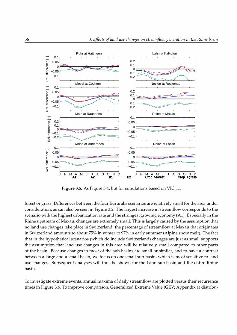
56 3. Effects of land use changes on streamflow generation in the Rhine basin
−0.1−0.05
00.050.1
Ruhr at Hattingen
Rel
. diff
eren
ce [−
]
A1 A2 B1 B2 Crop−>forest Crop−>grass
−0.2−0.1
00.10.2
Lahn at Kalkofen
A1 A2 B1 B2 Crop−>forest Crop−>grass
−0.1−0.05
00.050.1
Mosel at Cochem
Rel
. diff
eren
ce [−
]
A1 A2 B1 B2 Crop−>forest Crop−>grass
−0.2−0.1
00.10.2
Neckar at Rockenau
A1 A2 B1 B2 Crop−>forest Crop−>grass
−0.2−0.1
00.10.2
Main at Raunheim
Rel
. diff
eren
ce [−
]
A1 A2 B1 B2 Crop−>forest Crop−>grass
−0.1−0.05
00.050.1
Rhine at Maxau
A1 A2 B1 B2 Crop−>forest Crop−>grassJ F M A M J J A S O N D
−0.1−0.05
00.050.1
Rhine at Andernach
Rel
. diff
eren
ce [−
]
A1 A2 B1 B2 Crop−>forest Crop−>grassJ F M A M J J A S O N D
−0.1−0.05
00.050.1
Rhine at Lobith
A1 A2 B1 B2 Crop−>forest Crop−>grass
Figure 3.5: As Figure 3.4, but for simulations based on VICorg.
forest or grass. Differences between the four Eururalis scenarios are relatively small for the area under
consideration, as can also be seen in Figure 3.2. The largest increase in streamflow corresponds to the
scenario with the highest urbanization rate and the strongest growing economy (A1). Especially in the
Rhine upstream of Maxau, changes are extremely small. This is largely caused by the assumption that
no land use changes take place in Switzerland: the percentage of streamflow at Maxau that originates
in Switzerland amounts to about 75% in winter to 97% in early summer (Alpine snow melt). The fact
that in the hypothetical scenarios (which do include Switzerland) changes are just as small supports
the assumption that land use changes in this area will be relatively small compared to other parts
of the basin. Because changes in most of the sub-basins are small or similar, and to have a contrast
between a large and a small basin, we focus on one small sub-basin, which is most sensitive to land
use changes. Subsequent analyses will thus be shown for the Lahn sub-basin and the entire Rhine
basin.
To investigate extreme events, annual maxima of daily streamflow are plotted versus their recurrence
times in Figure 3.6. To improve comparison, Generalized Extreme Value (GEV; Appendix 1) distribu-

3.4. VIC model simulations for the entire basin 57
1 3 5 7 9 111315
50
100
150
200
Return period [years]
Q [m
3 s−
1 ]
Lahn at Kalkofen
1 3 5 7 9 111315
5000
6000
7000
8000
9000
10000
Return period [years]
Rhine at Lobith
Current Eur. A1 Eur. A2 Eur. B1 Eur. B2 Forest Grass
Figure 3.6: Annual maximum streamflow versus their recurrence time for the
Lahn sub-basin and the entire Rhine basin. A Generalized Extreme Value (GEV)
distribution is fitted through the data points. Six scenarios are plotted (4 Eururalis
scenarios, and crop replaced by resp. forest and grass, as well as the current
situation).
tions are fitted through the data points using maximum likelihood estimation. However, considering
the short period, they are not extrapolated to higher recurrence times. A similar analysis for low
flows is presented in Figure 3.7. Here, a low-flow event is defined as the cumulative deficit volume of
streamflow below a threshold (i.e. the event stops at the moment the threshold is exceeded; Fleig et al.
(2006)). The annual maximum values of the cumulative deficit volume are then plotted versus their
recurrence times. As a threshold, the 30th percentile of streamflow is selected. This value is a trade-off
between the amount of years without any event and the number of multi-year events, which both
affect the analysis ((Fleig et al., 2006)). A suitable and widely used limit distribution for excesses over
a threshold is the Generalized Pareto distribution (see Fleig et al. (2006), and Appendix 1). Therefore,
this distribution is fitted to the data points in Figure 3.7, again using maximum likelihood estimation.
Similar to Figure 3.4, the difference between peak magnitudes across the scenarios is small over the
entire basin (within a few percent). Over the entire range of return periods, the Eururalis scenarios
slightly increase the magnitude of the peak flows (especially A1 and A2). Conversion to forest and
grass slightly decreases this magnitude. Differences between extreme low flow periods are barely
visible when the entire basin is considered. At the sub-basin scale, differences in peak magnitudes
are slightly larger: all Eururalis scenarios increase peak flows, whereas afforestation leads to a small
decrease. Conversion to grassland hardly makes a difference. For extreme low flows in the Eururalis
scenarios a very small reduction in deficit volume (i.e., some alleviation of the low flow event) ap-

58 3. Effects of land use changes on streamflow generation in the Rhine basin
1 3 5 7 9 1113150
0.2
0.4
0.6
0.8
1
1.2
Return period [years]
Cum
. def
icit
[108 m
3 ]
Lahn at Kalkofen
1 3 5 7 9 1113150
20
40
60
80
100
Return period [years]
Rhine at Lobith
Current Eur. A1 Eur. A2 Eur. B1 Eur. B2 Forest Grass
Figure 3.7: Annual maximum cumulative non-exceedences of the 30th percentile
of streamflow versus their recurrence time for the Lahn sub-basin and the entire
Rhine basin. A Generalized Pareto (GP) distribution is fitted through the data
points. Six scenarios are plotted (4 Eururalis scenarios, and crop replaced by resp.
forest and grass, as well as the current situation).
pears for the low return times. Towards longer return times, on the other hand, low flows are slightly
enhanced. Conversion to cropland and grassland, on the other hand, reduces the deficit volume es-
pecially toward longer return periods. This can be explained by the fact that a large portion of the
extra streamflow in the Eururalis scenarios is surface runoff, which is absent in dry periods. Forest,
and to a smaller degree grass, sustain more baseflow in late summer, which is when most extreme
low flows occur. The same analyses were also carried out for the original VIC model source-code,
however, they are not shown here because they produced to a large extent the same results. Only
for the conversion to grassland results differed in a similar way to the mean streamflow differences
described above (Figure 3.5), i.e., grassland reduced extreme events even more than afforestation.
As can be seen from the data points in Figures 3.6 and 3.7, not all individual extremes behave the
same. This is further illustrated in Tables 3.4 and 3.5, which shows differences between the scenarios
for the five most extreme peak flows and low flows at Kalkofen and Lobith. Peak flows were selected
from the daily streamflow record of the reference simulation, under the constraint that peaks should
be two weeks apart to ensure independence, whereas low flows were selected based on the lowest
monthly means, which are selected to be 5 months apart. From Tables 3.4 and 3.5, it appears that at a
smaller scale (the Lahn basin), land use changes have varying effects on individual peak flows: there
is a wide range of differences in magnitude of the changes, from none at all to about 12% and even

3.4. VIC model simulations for the entire basin 59
Table 3.4: Five most extreme flood peaks and low flows at Kalkofen (outlet of the
Lahn basin), selected according to the reference situation, and the relative differ-
ence between six scenarios (Eururalis A1, A2, B1, B2, and cropland replaced by
forest and grass) and the reference situation for each event. Positive values denote
an increase with respect to the reference situation. For peak flows the magnitude
of the peak is considered. Low flow periodswere selected based on theminimum
monthly discharge value. the mean discharge over a 5-month window centered
around this minimum monthly mean discharge is then used to compare the land
use scenarios. Simulations are based on the modified VIC model.
Lahn at Kalkofen: peak flows
Date of max. 10-04-94 31-01-95 29-01-94 19-02-95 22-03-94
Magnitude [m3s−1] 188.70 163.59 162.25 150.22 148.16
A1 [%] 0.10 9.55 2.40 -2.98 0.08
A2 [%] 0.71 7.88 3.14 -1.81 1.46
B1 [%] -1.69 5.57 2.20 -3.90 -0.73
B2 [%] -0.25 7.25 2.18 -3.13 0.08
Forest [%] -12.34 -6.94 -2.26 -7.82 -11.89
Grass [%] -0.63 -3.64 -0.74 -2.82 -1.61
Lahn at Kalkofen: low flow periods
Month of min. 11-95 10-97 11-96 10-01 09-03
Monthly min. [m3s−1] 2.20 3.27 3.38 3.40 3.96
5-month mean [m3s−1] 3.66 4.58 6.74 6.20 6.33
A1 [%] 20.49 30.68 24.80 23.49 15.71
A2 [%] 14.33 19.07 17.16 16.78 10.24
B1 [%] 7.08 15.22 11.89 14.56 4.97
B2 [%] 11.45 19.05 15.80 17.35 8.61
Forest [%] -26.31 -6.68 -9.97 -1.04 -19.95
Grass [%] -19.78 -9.87 -7.27 -2.57 -15.32
directions are not consistent. Low flows, on the other hand, are relieved by the Eururalis scenarios
to some extent because of increasing streamflow. However, discharge in the Lahn nearly disappears
during extreme low flows (e.g. about 3.5 m3s−1 in November 1995). Therefore, in an absolute sense
differences are still very small. Conversion to forest or grassland mainly reduces streamflow due to
enhanced evapotranspiration. When the entire basin is considered, the same effects can be seen as in
the Lahn, although changes are much smaller, mainly within 5%.
Finally, spatial patterns of differences in surface runoff and soil moisture between all six scenarios
are displayed in Figures 3.8 and 3.9. For the Eururalis scenarios, surface runoff mainly increases in
the areas that show the highest urbanization (Figure 3.2), i.e., the Ruhr area close to Lobith, along

60 3. Effects of land use changes on streamflow generation in the Rhine basin
Table 3.5: As Table 3.4, but for Lobith, the outlet of the entire Rhine basin.
Rhine at Lobith: peak flows
Date of max. 27-02-99 02-02-95 29-03-01 28-03-02 03-02-94
Magnitude [m3s−1] 8111 8015 7834 7685 7173
A1 [%] 3.56 4.27 3.34 2.49 1.18
A2 [%] 2.58 3.54 2.58 2.05 0.90
B1 [%] 2.04 2.30 1.72 1.27 0.85
B2 [%] 2.04 2.52 1.83 1.35 0.73
Forest [%] -1.27 -2.55 -1.71 -1.61 -0.04
Grass [%] -1.23 -1.43 -1.19 -1.09 -0.51
Rhine at Lobith: low flow periods
Month of min. 10-95 09-01 01-97 02-98 03-96
Monthly min. [m3s−1] 1123 1130 1149 1190 1231
5-month mean [m3s−1] 1512 1617 1984 2150 1529
A1 [%] 2.77 3.56 4.91 3.64 3.14
A2 [%] 2.06 2.45 3.45 2.60 2.46
B1 [%] 1.72 2.00 3.02 1.90 1.80
B2 [%] 1.63 2.02 3.01 1.95 1.79
Forest [%] -1.46 -0.03 -1.50 -1.50 -2.49
Grass [%] -1.83 -0.99 -1.43 -2.12 -1.97
the main Rhine branch and in the Neckar sub-basin. In the scenarios where cropland was replaced
by forest or grass, changes in surface runoff occur only locally at a few distinct spots, although in
both scenarios land cover over an extensive area is changed. This, of course, is very much related to
soil type and topography: surface runoff decreases in most of the basin, especially in the more sandy
parts, whereas it increases in the mountainous southern part. When cropland is converted to grass,
the same can be seen to a smaller extent. Because surface runoff is only caused by saturation in the
VICmodel, increases in surface runoff are correlated with increases in soil moisture. As can be seen in
Figures 3.9 and 3.8, increases in both soil moisture and surface runoff are concentrated in the western
part of the basin for the hypothetical scenarios. This area has a more loamy soil texture than many
other areas covered with cropland, delaying the discharge of water through baseflow and increasing
soil moisture contents. Apart from the western part, soil moisture contents mainly decrease in the
remaining zones were cropland was converted to (semi-)natural land. Also in the Eururalis scenarios,
the increases in surface runoff are associatedwith increases in soil moisture, which in turn correspond
to urbanizing areas.

3.5. Summary and conclusions 61
Figure 3.8: Spatial pattern of absolute differences in surface runoff between the
six scenarios and the current situation. Positive values indicate an increase with
respect to the current situation. Results for VICmod are shown.
3.5 Summary and conclusions
In this study, we have investigated the effects of land use changes on average streamflow, as well as
extreme floods and low flows for various locations in the Rhine basin. Land use projections for the
year 2030 were used, according to four IPCC emission-scenarios. In addition, to investigate the sensi-
tivity of streamflow to land use change, some extreme, hypothetical scenarios were devised, where all
cropland throughout the basin was replaced by either forest or grass. All land use change scenarios
were simulated using the VIC model, which has the advantage that the evapotranspiration routine is
physically based and does not require specific calibration parameters. All simulations were carried
out using the same atmospheric forcing dataset, which spans the period of 1994 through 2003. Effects
of climate change are not taken into account in this study. In later research, therefore, it would be in-
teresting to investigate whether land use change effects are different under a different climate regime.
Besides the simulations covering the entire Rhine basin, another set of simulations was carried out
covering a single VIC pixel completely covered with six different land use types.

62 3. Effects of land use changes on streamflow generation in the Rhine basin
Figure 3.9: As Figure 3.8, but now differences in total soil moisture storage are
plotted.
From the latter simulations, it appears that the current version of the VIC model is not completely
suitable to simulate differences in land use types, mainly because of the fact that no bare soil evap-
oration is allowed when a land use tile is classified as vegetated. Especially in winter this leads to
underestimations of evapotranspiration, which is confirmed by Hurkmans et al. (2008), where a com-
parison between evapotranspiration from a VIC pixel and a lysimeter (their Figure 11) indeed shows
severe underestimations by the VICmodel in winter. By introducing a fractional bare soil evaporation
in vegetated areas, the representation of bare soil evaporation and transpiration is more realistic and
the annual cycle for grass is represented more accurately compared to the lysimeter data. The total
amount of evapotranspiration is slightly higher but not unrealistic (seeVerstraeten et al. (e.g. 2005) and
the lysimeter data mentioned before).
From the simulations covering the entire Rhine basin, the effects of different land use change scenar-
ios on mean streamflow are similar for both the original and modified VIC model, suggesting that
they are fairly robust and independent on the model formulation of the VIC model. The effects are

3.5. Summary and conclusions 63
small when considering streamflow at the basin outlet (within 5%, both in mean and extreme stream-
flow), because in the Eururalis scenarios the affected areas are relatively small and the contribution
from Switzerland can be considerable, especially in spring season. In general, the future land use
scenarios (Eururalis) indicate an increase in streamflow, mainly due to urbanization. Effects of ur-
banization are quite small, however, because they are partly compensated by a decrease of cropland
and small increases in grassland, forest and natural area (e.g. shrubs). The more extreme, hypo-
thetical scenarios, on the other hand, indicate a decrease of streamflow. Conversion of cropland to
grass reduces streamflow nearly as much as conversion to forest. This, however, is partly caused by
an overestimation of interception evaporation for grass in the model that was discussed in Section 3.3.
For management purposes, i.e., mitigating extreme floods and low flows, land use changes can have
local effects and can affect streamflow from small tributaries significantly. As far as influencing the
magnitude and timing of peaks arriving at Lobith are concerned, however, effects are small. In dif-
ferent areas, different types of land use changes would be necessary. For example, only the relatively
small Lahn basin proved relatively sensitive to afforestation, because in the current situation the dom-
inant land use type is cropland. Therefore, afforestation has a relatively large influence. For each area,
specific land use changes, depending on the current dominant cover could be designed. In further
research, therefore, alternative scenarios should be taken into account for each sub-basin separately,
or for even smaller sub-basins. An effective combination of different land use changes in different
parts of the basin could be able to significantly alter the magnitude of low flows and/or the timing of
flood peaks at the basin outlet.
Acknowledgements
This research was supported by the European Commission through the FP6 Integrated Project NeWa-
ter and the BSIK ACER project of the Dutch Climate Changes Spatial Planning Programme. We thank
Daniela Jacob and Eva Starke from the Max Planck Institut fur Meteorologie, Hamburg, Germany for
providing the atmospheric forcing data. Rita Lammersen and Hendrik Buiteveld from Rijkswater-
staat Waterdienst, The Netherlands are kindly acknowledged for providing streamflow observations
and we thank the three anonymous reviewers for their constructive comments.


Chapter 4
Changes in streamflow dynamics in the Rhine basin during the 21st centuryunder different climate scenarios
This chapter is a modified version of: R. T. W. L. Hurkmans, W. Terink, R. Uijlenhoet, P. .J. J. F. Torfs, D. Jacob
and P. A. Troch (2009), “Changes in streamflow dynamics in the Rhine basin during the 21st century under different
climate scenarios”, submitted to J. Clim.

66 4. Changes in streamflow in the Rhine basin under climate scenarios
Abstract
Due to global warming, the hydrologic behavior of the Rhine basin is expected to shift from a combined
snowmelt and rainfall driven regime to a more rainfall dominated regime. Previous impact assessments
have indicated that this leads, on average, to increasing streamflow by ∼30% in winter and spring, and
decreasing streamflow by a similar value in summer. In this study, high-resolution (0.088◦) regional climate
scenarios for the Rhine basin are used to force a macro-scale hydrological model. These climate scenarios are
based on model output from the ECHAM5-OM global climate model, which is in turn forced by three SRES
emission scenarios: A2, A1B and B1. The Variable Infiltration Capacity model (VIC; version 4.0.5) is used
to examine changes in streamflow at various locations throughout the Rhine basin. Average streamflow,
peak flows, low flows and several water balance terms are evaluated for both the first and second half of
the 21st century. The results reveal a distinct contrast between those periods. The first half is dominated
by increased precipitation, causing increased streamflow throughout the year. During the second half of
the century, a streamflow increase in winter/spring and a decrease in summer is found, similar to previous
studies. This is caused by (1) temperature and evapotranspiration, which are considerably higher during the
second half of the century, (2) decreased precipitation in summer and (3) an earlier start of the snowmelt
season. Magnitudes of peak flows increase during both periods, that of streamflow droughts only during the
second half of the century.

4.1. Introduction 67
4.1 Introduction
According to the latest IPCC assessment report (IPCC, 2007), all currently available global climate
models agree on an increase in global mean temperature of 1.1◦C to 6.4◦C over the 21st century. Asso-
ciated with this global warming, the hydrological cycle is expected to intensify, causing precipitation
to fall in more extreme events (Trenberth, 1997a). In addition, higher air temperatures will cause more
precipitation to fall as rain instead of snow, and the snow melt season to start earlier in the year (Bar-
nett et al., 2005). As far as the Rhine basin is concerned, this amounts to an increase in temperature of
1.0◦C to 2.4◦C by 2050, causing the hydrological regime of the Rhine to shift from a combined rainfall
and snowmelt driven system to a more rainfall dominated system (Barnett et al., 2005; IPCC, 2007).
The Rhine basin is densely populated and heavily industrialized, and the river Rhine has the highest
traffic density in Europe as an inland waterway. Its water is used for many purposes, e.g. agriculture,
industry, domestic water supply and (hydro)power generation (Kwadijk and Rotmans, 1995;Middelkoop
et al., 2001). Because of all the economic value that is concentrated in the basin, it is very vulnerable
to hydrologic extremes, both floods and droughts (Kleinn et al., 2005). It is therefore not surprising
that many climate change impact assessments have been carried out for the Rhine basin in recent
years (e.g. Kwadijk and Middelkoop, 1994; Kwadijk and Rotmans, 1995; Middelkoop et al., 2001; Shabalova
et al., 2003; Pfister et al., 2004; Zierl and Bugmann, 2005; Lenderink et al., 2007). Most of these studies are
based on climate model output, which are based on scenarios describing greenhouse gas emissions.
Emission scenarios range from a simple doubling of CO2 concentrations (e.g. Middelkoop et al., 2001)
or a gradual increase of CO2 (for example 1% per year in Shabalova et al. (2003)) to the more complex
scenarios developed by IPCC in the Special Report on Emission Scenarios (SRES; IPCC, 2000). SRES-
scenarios are based on several alternative developments of energy technology and contain not only
CO2, but also other greenhouse gases and aerosols. Because the spatial resolution of global climate
models (GCM) is generally too low for hydrological applications (> 100 km), downscaling occurs ei-
ther by statistical methods (as was done for example by Kwadijk and Middelkoop (1994); Kwadijk and
Rotmans (1995)), or by nesting a regional climate model (RCM) in the GCM over the domain of inter-
est (e.g. Shabalova et al., 2003; Middelkoop et al., 2001; Kleinn et al., 2005). The downscaled climate data
are then fed to some hydrological model to obtain river discharges. All the assessments mentioned
above qualitatively agree in their results. More discharge is projected in winter and spring because of
increased precipitation and snow melt (+30% according to Lenderink et al. (2007) and Shabalova et al.
(2003)), and less discharge in summer because of increased evapotranspiration, less snow buffering
and decreased precipitation (−30% to −40% according to the same studies).
In the studies described above, most of the employed regional climate scenarios have spatial reso-
lutions of 25 to 50 km. By means of a second downscaling step higher spatial resolutions can be
obtained. From the Max Planck Institut fur Meteorologie (MPI-M) in Hamburg, Germany, climate
scenarios are available for the Rhine basin at a spatial resolution of 0.088◦ (∼ 10 km). These scenarios
are based on the GCM ECHAM5-OM and downscaled in two steps by the regional climate model

68 4. Changes in streamflow in the Rhine basin under climate scenarios
REMO (Jacob, 2001). To capture extreme precipitation events, and thus also extreme peak flow events,
a high spatial resolution is important because extreme precipitation is usually convective in nature
and its spatial extent relatively small. Moreover, as part of the catchment is very mountainous, orog-
raphy is relatively complex and a high model resolution allows more of this complexity to be resolved
explicitly. An additional advantage of the climate scenarios used in this study is the fact that they are
transient, spanning the entire 21st century. The studies that were mentioned above typically used a
timeslice of 30 years, often the period 2071–2100.
In this study, we employ three high-resolution climate change scenarios, according to three SRES sce-
narios: B1, A1B and A2. We compare the scenarios with results of a reference model run spanning
the period 1950-2000. All atmospheric time series are corrected for their model bias based on obser-
vations of precipitation and temperature (Section 4.3.1). As a macro-scale hydrological model, we use
the Variable Infiltration Capacity (VIC; Liang et al., 1994). This model was applied to the Rhine basin
at a spatial resolution of 0.05◦ (∼ 5.5 km), as described by Hurkmans et al. (2008). Compared to other
models that are typically used for climate change impact studies and which are generally more sim-
ple, VIC has the advantages that (1) its parameterization of evapotranspiration is physically based,
(2) it has a detailed description of snow accumulation and melt processes and (3) sub-grid variabil-
ity of land use, elevation and infiltration is taken into account. For these reasons, VIC was found to
be less sensitive to parameter settings than the more simple water balance models mentioned above
(Hurkmans et al., 2008). This is an important advantage because it is questionable whether conceptual
model parameters determined under current climate conditions will be valid throughout the 21st cen-
tury under a changing climate. From the model results, we investigate the effect of climate change on
average and extreme streamflow, both in terms of peak flows and streamflow droughts. By analyzing
streamflow at several locations throughout the river basin and the distributed model results, the spa-
tial pattern of the effects of climate changes is investigated. Finally, changes in various components
of the water balance, such as evapotranspiration, snow melt and baseflow, are analyzed.
4.2 Data and model
4.2.1 Study area
The Rhine basin is a major river in western Europe. It originates in the Swiss Alps and drains portions
of Switzerland, Germany, France and TheNetherlands before draining in theNorth Sea. The total area
covered is about 185,000 km2. After crossing the German-Dutch border at Lobith, the river splits into
three branches. Therefore, we only take into account the area upstream of Lobith (Figure 1.5). As
was mentioned before, the discharge of the Rhine is a combination of rainfall and snowmelt. Snow is
concentrated in the Alpine part of the area, where elevations range up to about 4000 m.a.s.l. For more
information about the Rhine basin, see Section 1.2.

4.2. Data and model 69
4.2.2 Hydrological model
The Variable Infiltration Capacity model (VIC; Liang et al., 1994) is a distributed, macro-scale hydro-
logical model. It is developed to provide land surface boundary conditions for climate models, and
therefore solves evapotranspiration and the associated turbulent fluxes in a physically based way.
The coupled water- and energy balances are solved, in combination with the Penman-Monteith equa-
tion (Penman, 1948; Monteith, 1965), to calculate evapotranspiration. Sub-grid variability in land use
and elevation is accounted for by dividing each grid cell in tiles based on fractional areal coverage.
Sub-grid variability of topography is accounted for by means of an exponential relation between the
fraction of the grid cell that is saturated and the infiltration capacity. The soil column is divided in
three soil layers. Drainage from the surface to the lowest layer is gravity-driven and downwards only.
Baseflow depends on the soil moisture content of the lowest soil layer through a function that consists
of a linear and a non-linear segment. Routing of baseflow and surface runoff occurs through a simple
algorithm developed by Lohmann et al. (1996), which was applied in combination with VIC before
(e.g. Lohmann et al., 1998a,b). The VIC model is described more extensively in Section 1.3. The VIC
model has been used in previous studies as a land surface parameterization in climate models (e.g.
Lohmann et al., 1998c; Pitman et al., 1999; Liang et al., 1998), but also for hydrological purposes. For ex-
ample, Hamlet et al. (2007) used the model for climate variability impact assessments and Matheussen
et al. (2000) and Hurkmans et al. (2009a) investigated land use changes using VIC. Also Nijssen et al.
(1997) andNijssen et al. (2001) successfully applied VIC for streamflow simulation in large river basins.
The VIC model was applied to the Rhine basin in a previous study (Hurkmans et al., 2008), at a spatial
resolution of 0.05◦ and a temporal resolution of 3 hours. Two modifications of the VIC model that
were introduced in a recent study dealing with land use changes (Hurkmans et al., 2009a), are used in
this study as well. First, in sparsely vegetated areas bare soil evaporation is allowed to occur simulta-
neous to transpiration and canopy evaporation. Second, a parameter is introduced in urban areas to
increase the amount of surface runoff relative to baseflow. For more details about these modifications,
we refer to Hurkmans et al. (2009a). Atmospheric forcing for the model is described in Section 4.2.3.
Land use data were obtained from the PELCOM project (Mucher et al., 2000) at a spatial resolution of
1 km, and soil data are taken from the global FAO dataset described by Reynolds et al. (2000). Based on
percentages of sand and clay from this dataset soil textures are classified and the default parameters
from the VIC website1 are assigned to each class.
4.2.3 Atmospheric data
All atmospheric datasets that are used in this study are model output from the Regional climate model
REMO (Jacob, 2001) as provided by the Max Planck Institut fur Meteorologie (MPI-M) in Hamburg,
Germany. A validation dataset, a reference dataset and three scenarios datasets were available. The
main characteristics of all datasets are shown in Table 4.1, and the way they are used in this study is
1http://www.hydro.washington.edu/Lettenmaier/Models/VIC/VIChome.html

70 4. Changes in streamflow in the Rhine basin under climate scenarios
Table 4.1: Overview of atmospheric datasets used in this study.
Dataset Driving model Spatial res. Time res. Period
Validation ECMWF 0.088 hourly 1979–2003
Reference ECHAM5-OM 0.088 hourly 1950–2000
Scenarios ECHAM5-OM 0.088 hourly 2001–2100
Observations - sub-basin daily 1961–1995
shown schematically in Figure 4.1. The validation dataset is an extended version of the atmospheric
dataset that was used in Hurkmans et al. (2008) and Hurkmans et al. (2009a). It is based on the global
ERA15 re-analysis dataset (ECMWF Re-Analysis2, 1979–1993), extended up to 2003 using operational
ECMWF analysis data. Because the ERA data are (partly) based on observations, this data can be
used to calibrate the hydrological model, as was done in Hurkmans et al. (2008). The reference dataset
is based on a REMO model run driven by the general circulation model ECHAM5-OM, as are the
three scenario datasets. Because the reference dataset is not constraint by observations, it only resem-
bles the current climate in a statistical sense. It can, therefore, not be used for hydrological model
calibration. Because it is based on the same models as the scenarios, it can be compared with the
scenarios to obtain a climate change signal. This is not the case for the validation dataset because it is
based on a different driving model (i.e. ERA-data).
The spatial resolutions of both ERA and ECHAM5-OM data is too low for hydrological applications
(> 100 km). They are, therefore, dynamically downscaled using the REMOmodel in two steps. First,
intermediate REMO output with a resolution of 0.44◦ (about 50 km) is obtained, which is downscaled
using a second step to 0.088◦ (about 10 km; Jacob et al., 2008) and personal communication with S.
Kotlarski, (MPI-M).
Both driving “models”, ERA-data and ECHAM5-OM, have structural modeling errors comparedwith
observations. Prior to using the data, this model bias needs to be corrected for using observations.
Interpolated observations were available over the Rhine basin (Sprokkereef , 2001a) for this purpose.
Because the spatial and temporal resolutions of these observations are too low, they cannot be used
to force the VIC model. Therefore, we use the validation and reference datasets described above to
represent the current climate conditions. The bias corrections are described in detail in Section 4.3.1.
For both driving models a separate bias correction is needed. Because the three scenario datasets are
based on the same modeling chain as the reference dataset, we assume that the model bias is similar
for both the reference dataset and the scenarios and apply the same correction to both.
The three scenarios are based on three different CO2 emission scenarios as defined by the IPCC in
the Special Report on Emission Scenarios (SRES; IPCC, 2000): the A2, A1B and B1 scenarios. Each of
those scenarios is based on a storyline of energy and technology development. The A2 scenario refers
2http://www.ecmwf.int

4.3. Methodology 71
to a world with continuously growing population and very regionally oriented economic growth.
A1B refers to a globalized, very rapidly growing economy with fast introduction of new technologies
that are balanced between fossil fuel-intensive and sustainable and clean. Population in A1B grows
rapidly until the middle of the century and declines thereafter. B1, finally, refers to a globalized,
rapidly growing population, but with changes in economic structure with an environmental empha-
sis, and fast introduction of clean and efficient technologies. For more details about these storylines,
see Section 1.1.3 and IPCC (2000).
Figure 4.1: Schematic representation of all datasets used in this study and how
they are used.
4.3 Methodology
4.3.1 Bias correction
A problem with the use of RCM output is the fact that simulated precipitation and temperature differ
systematically from observed values (Christensen et al., 2008). These biases can vary among RCMs and
are also geographically dependent (Jacob et al., 2007), and to obtain realistic streamflow simulations
in the present climate, they should be corrected (Lenderink et al., 2007). Different methods exist to
correct for these biases. For example, Lenderink et al. (2007) used a spatially and seasonally varying
correction factor, and Hay et al. (2002) used the Gamma distribution to match observed and simulated
precipitation values. In this study, we use a relatively simple method that was applied to the Meuse
basin by Leander and Buishand (2007). In addition, Shabalova et al. (2003) applied it to the Rhine basin to

72 4. Changes in streamflow in the Rhine basin under climate scenarios
obtain a plausible climate scenario. An advantage of this method is that not only the mean, but also
the temporal variability is corrected. The method corrects precipitation and temperature separately,
and leaves other input variables for VIC (i.e., radiation, humidity, wind speed and air pressure) unaf-
fected. Because no observations are available for these variables at this scale and resolution, it is not
possible to correct for them. Moreover, the effect on the resulting streamflow of errors occurring in
these variables are relatively small compared to biases in precipitation and temperature. Observed
precipitation and temperature for the period 1961–1995 are available on a daily basis for each of 134
sub-catchments in the Rhine basin (Sprokkereef , 2001a). Therefore, and because the model bias was
found to vary spatially (in accordance with Leander and Buishand (2007) and Lenderink et al. (2007)), the
bias correction is applied to daily average temperature and daily accumulated precipitation, for each
sub-basin individually.
Because the reference dataset and validation datasets (Table 4.1) are based on different models, a bias
correction is applied to both datasets separately. For both corrections, the maximum period of over-
lap between data and observations is used to estimate the correction parameters. For the validation
dataset, this period is 1979–1995, whereas for the reference dataset it is 1961–1995. For both pre-
cipitation and temperature, a 5-day climatology is derived from observations and model output by
calculating the average and standard deviation over all available years, i.e., 17 years for the validation
and 35 years for the reference dataset. A window of 30 days before and 30 days after the considered
5-day period is used to calculate the “smoothed” average and standard deviation. The average and
standard deviation are thus calculated over 65 x 17 (validation dataset), or 65 x 35 (reference dataset)
data points. The correction is applied separately for each of the 73 5-day periods in the resulting cli-
matology.
Precipitation is corrected according to a non-linear function (Leander and Buishand, 2007):
P ∗ = aP b, (4.1)
where P is the uncorrected precipitation, P ∗ the corrected precipitation and a and b are two parame-
ters. First, b is fitted for the coefficient of variation (CV) of the modeled precipitation to match the CV
of the observed precipitation. Second, a is fitted such that the average modeled precipitation fits the
average of the observed precipitation (using the value of b obtained in the first step).
The correction of temperature is done in a linear way, based on the mean and standard deviation. For
each sub-basin, the corrected daily temperature T ∗
mod is calculated as:
T ∗
mod = T obs +σ (Tobs)
σ (Tbasin)
(
Tmod − T obs
)
+(
T obs − T basin
)
, (4.2)
where Tmod is the uncorrected daily modeled temperature, Tobs is the observed daily average temper-
ature for a sub-basin, and Tbasin is the modeled sub-basin average temperature. In Equation 4.2 an
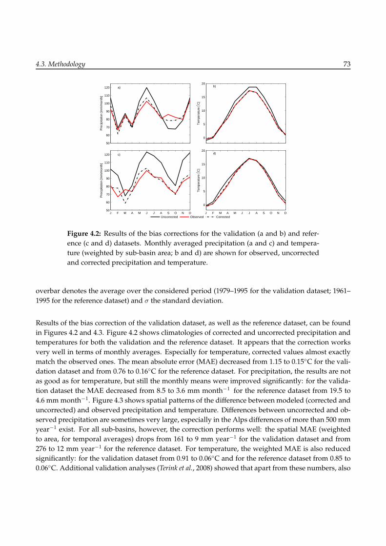
4.3. Methodology 73
50
60
70
80
90
100
110
120
Pre
cipi
tatio
n [m
m/m
onth
]
a)
0
5
10
15
20
Tem
pera
ture
[° C]
b)
J F M A M J J A S O N D50
60
70
80
90
100
110
120
Pre
cipi
tatio
n [m
m/m
onth
]
c)
J F M A M J J A S O N D
0
5
10
15
20
Tem
pera
ture
[° C]
d)
Uncorrected Observed Corrected
Figure 4.2: Results of the bias corrections for the validation (a and b) and refer-
ence (c and d) datasets. Monthly averaged precipitation (a and c) and tempera-
ture (weighted by sub-basin area; b and d) are shown for observed, uncorrected
and corrected precipitation and temperature.
overbar denotes the average over the considered period (1979–1995 for the validation dataset; 1961–
1995 for the reference dataset) and σ the standard deviation.
Results of the bias correction of the validation dataset, as well as the reference dataset, can be found
in Figures 4.2 and 4.3. Figure 4.2 shows climatologies of corrected and uncorrected precipitation and
temperatures for both the validation and the reference dataset. It appears that the correction works
very well in terms of monthly averages. Especially for temperature, corrected values almost exactly
match the observed ones. The mean absolute error (MAE) decreased from 1.15 to 0.15◦C for the vali-
dation dataset and from 0.76 to 0.16◦C for the reference dataset. For precipitation, the results are not
as good as for temperature, but still the monthly means were improved significantly: for the valida-
tion dataset the MAE decreased from 8.5 to 3.6 mm month−1 for the reference dataset from 19.5 to
4.6 mmmonth−1. Figure 4.3 shows spatial patterns of the difference between modeled (corrected and
uncorrected) and observed precipitation and temperature. Differences between uncorrected and ob-
served precipitation are sometimes very large, especially in the Alps differences of more than 500 mm
year−1 exist. For all sub-basins, however, the correction performs well: the spatial MAE (weighted
to area, for temporal averages) drops from 161 to 9 mm year−1 for the validation dataset and from
276 to 12 mm year−1 for the reference dataset. For temperature, the weighted MAE is also reduced
significantly: for the validation dataset from 0.91 to 0.06◦C and for the reference dataset from 0.85 to
0.06◦C. Additional validation analyses (Terink et al., 2008) showed that apart from these numbers, also

74 4. Changes in streamflow in the Rhine basin under climate scenarios
Figure 4.3: Results of the bias corrections in terms of spatial patterns. Each map
shows the difference between corrected or uncorrected data versus observations.
Differences in mean annual temperature and mean cumulative precipitation are
shown, for both the validation (upper four panels) and reference datasets (lower
four panels). Positive values indicate an overestimation with respect to the ob-
servations.
other statistics, such as the extreme values (low exceedence probabilities), the lag-1 autocorrelation
and the number of wet days in the corrected datasets improved with respect to the uncorrected ones.
4.3.2 Model calibration
The bias-corrected validation dataset is used to calibrate VIC. Because the calibration process is com-
putationally quite demanding, we calibrated the model on a relatively short period: 1994–1997. For
each simulation, 1993 is used to initialize the model. The remainder of the validation dataset (1998–
2003) is used to validate the model. The model was calibrated in a similar way as described in Hurk-
mans et al. (2008), using 5 calibration parameters (for details, see Hurkmans et al. (2008)) and a numer-
ically efficient algorithm to optimize them simultaneously, the Downhill-Simplex algorithm (Nelder
and Mead, 1965). The Nash-Sutcliffe model efficiency (Nash and Sutcliffe, 1970) was used as objective
function. A difference with the application described in Hurkmans et al. (2008) is the fact that in this
study, the model was calibrated for each of seven zones separately, including five of the largest tribu-
taries. These zones are shown in Figure 1.5. Calibration and validation results for the entire basin and

4.4. Results 75
Table 4.2: Characteristics of observed streamflow and calibration and validation
results for five of the main tributaries of the Rhine (Ruhr, Lahn, Main, Mosel
and Neckar), and three locations along the main branch of the Rhine: Maxau,
Andernach and Lobith. Mean, maximum, and mean annual maximum (Qmam)
streamflow are all calculated for the period 1990-2005 (the extent of the database
that is available). For the calibration period (1994–1997) and the validation period
(1998–2003), the correlation coefficient (ρ, Nash-Sutcliffe modeling efficiency (E),
and the relative volume error (RVE) are shown.
Observed Calibration Validation
Sub-catchment Station Qmean Qmax Qmam ρ E RVE ρ E RVE
- - [m3s−1] [m3s−1] [m3s−1] [-] [-] [%] [-] [-] [%]
Ruhr Hattingen 72.6 867.0 579.4 0.58 0.22 34.57 0.61 0.30 27.58
Lahn Kalkofen 46.0 587.4 373.0 0.80 0.59 -13.37 0.61 0.27 -7.31
Main Raunheim 175.2 1990.8 1053.3 0.81 0.65 -7.25 0.69 0.42 -7.95
Mosel Cochem 338.6 4008.9 2492.3 0.71 0.49 1.21 0.69 0.37 12.02
Neckar Rockenau 142.6 2105.4 1326.0 0.54 0.07 23.14 0.61 -0.15 35.84
Rhine Maxau 1278.3 4427.8 3269.5 0.59 0.10 11.20 0.50 -0.81 26.82
Rhine Andernach 2076.0 10460.0 7274.3 0.75 0.55 5.03 0.62 0.17 15.72
Rhine Lobith 2239.9 11774.6 7655.3 0.81 0.59 11.69 0.70 0.22 19.77
the main tributaries are shown in Table 4.2.
From Table 4.2, it appears that especially for mountainous areas such as the Rhine upstream of Maxau
and the Neckar, performance indicators are relatively low. This can have several reasons: first, the
model was forced by REMO model output, as was discussed previously. Differences between obser-
vations and this modeled data are at times quite large, as was also pointed out by Hurkmans et al.
(2008), who compared the datasets extensively. Even though the structural error or bias was largely
removed by the bias correction (see Section 4.3.1), the variation over time was not changed and sig-
nificant differences between observed and modeled precipitation time series persisted. Second, the
complex topography in the mountainous areas complicates hydrological modeling due to the high
amount of small-scale heterogeneity. Third, there are some large surface reservoirs present in the
Alpine part, such as the Bodensee, which are not included in the model but can damp peaks in the
hydrograph considerably.
4.4 Results
The calibrated VIC model is now used to simulate streamflow for the reference period and the three
climate scenarios described in Section 4.2.3 using the bias-corrected atmospheric data. Figure 4.4

76 4. Changes in streamflow in the Rhine basin under climate scenarios
shows annual time series of the annual mean, minimum and maximum streamflow at the basin
outlet, Lobith. For the reference period and the A2-scenario also the 10th and 90th percentiles are
shown. Thus, Figure 4.4 shows in a qualitative manner the trends in average, minimum and maxi-
mum streamflow during the 21st century for all scenarios and the reference period. A striking feature
is the fact that there seems to be a decreasing trend both in minimum and maximum streamflow, par-
ticularly during the period 2052–2100. However, annual maxima are higher than they are during the
reference period throughout the 21st century. From the simulated records, the years 1951 and 2001
are used to initialize the model for the reference period and the scenarios respectively. To be able
to compare three periods of equal length, also 2051 is discarded, yielding three periods spanning 49
years each. In Sections 4.4.2 and 4.4.4 we investigate the differences between the periods 2002–2050
and 2052–2100 on one hand, and 1952-2000 on the other hand, in more detail.
1960 1980 2000 2020 2040 2060 2080 21000
2000
4000
6000
8000
10000
12000
14000
16000
Dis
char
ge [m
3 s−
1 ]
Reference A2 A1B B1
Figure 4.4: Time series of annual mean (middle solid lines), maximum (upper
lines) and minimum (lowest lines) daily streamflow at Lobith for all datasets.
For the A2-scenario and the reference situation, the shaded area represents area
between the 10th and 90th percentiles.
4.4.1 Spatial patterns of atmospheric variables
To help interpreting the changes in streamflow that are discussed later in this paper, spatial patterns
of the differences in precipitation, evapotranspiration and air temperature are plotted in Figures 4.5,
4.6 and 4.7 respectively. Temperature and precipitation are used to force the VIC model and are bias-
corrected (Section 4.3.1), evapotranspiration is simulated by the model. Only differences between the
period 2052–2100 and the reference period are shown, both for the winter (DJF) and summer season
(JJA). Figure 4.5 shows precipitation increases in winter and decreases in summer for all scenarios.
The largest increases in precipitation during the winter season are found in the northern and western

4.4. Results 77
Figure 4.5: Difference in annual mean precipitation between three climate scenar-
ios for the period 2052-2100 and the reference situation (1952–2000). The upper
three panels show differences in the winter season (DJF), the lower three panels
for the summer season (JJA).
part, as well as the mountainous area of the Black forest and the Vogues mountains, located along the
southern part of the Rhine valley. The A2 scenario also shows increases in precipitation in the Alpine
part and in some areas in the eastern Rhine basin, whereas the B1 scenario does not. The A1B scenario
shows intermediate increases in those areas. In summer, the decrease in precipitation mainly occurs
in the Alpine part of the basin, the Neckar sub-basin and the southern part of the Mosel. The north-
ern part, the Black forest and the Vogues area still show small increases in precipitation. It should be
noted that the spatial pattern of the applied precipitation is influenced by our bias correction. Because
the correction was applied for each of 134 sub-basins separately, the overall spatial pattern is “drawn”
towards that of the observations to some extent (see Figure 4.3). In addition, because the same expo-
nent in Eq. 4.1 is applied to the reference dataset and the scenarios, differences between those can be
amplified or reduced locally.
Changes in actual evapotranspiration (Figure 4.6) are quite homogeneous in space during the winter
season: the entire basin, except the upper Alpine part experiences increases in evapotranspiration of

78 4. Changes in streamflow in the Rhine basin under climate scenarios
Figure 4.6: As Figure 4.5, but for actual evapotranspiration.
8 to 20 mm month−1. In summer, however, there are large regional differences. Large parts of the
western part (the Mosel area), as well as the eastern part (the Main) and a small area in northern
Switzerland show small decreases in evapotranspiration. Ideally, to confirm that these decreases are
caused by water limitation, one would want to see a similar plot of the potential evapotranspiration.
This, however, does not belong the standard VIC model output. Because of the parameterizations for
sub-grid variability in the model (Section 4.2.2) it is not trivial to extract this information, therefore
we used air temperature as a proxy for potential evapotranspiration (Figure 4.7). Radiation would be
another option to use as a proxy but we do not expect the spatial pattern of incoming radiation to be
very different from that of air temperature. The spatial pattern for temperature also looks quite homo-
geneous for both seasons, albeit that the warming is somewhat higher in the southern part, the valley
of the upper Rhine and the higher areas on either side. Assuming that potential evapotranspiration
follows a similar spatial pattern as temperature, this suggests that the decreasing evapotranspiration
values in summer could indeed be caused by water limitation.

4.4. Results 79
Figure 4.7: As Figure 4.5, but for air temperature.
4.4.2 Mean streamflow
Figure 4.8 shows the climatologies of relative differences in streamflow between each of the two
future periods and the reference period, at four locations in the Rhine basin, representing a small
(Ruhr) and a large (Main) tributary, the Alpine part (Maxau) and the entire basin (Lobith). The lower
panel of Figure 4.8 shows the absolute streamflow climatology for Maxau, which is dominated by
snowmelt. From this plot, it appears that during the period 2002-2050 the maximum monthly dis-
charge at Maxau, which occurs in June, does not change or slightly increases (for the A1B scenario).
The start of the melting season is slightly shifted to occur earlier in the year. During the second half of
the 21st century, however, the melting season starts about 6 weeks to 8 weeks earlier and maximum
discharge is significantly lower than during the reference period. In late summer (July to Septem-
ber), therefore, discharge is reduced considerably. The largest difference with the reference period is
reached in August and amounts to about 40% less discharge at Maxau. The A1B scenario shows the
most severe decrease in discharge. The earlier snowmelt in combination with increased precipitation
in winter and spring (Figures 4.9 and 4.10) causes increased discharge in these seasons. The increase
in winter and spring nearly offsets the decrease in summer: annual streamflow slightly (<10%) in-
creases for the A2 and B1 scenarios. For the A1B scenario the annual streamflow slightly decreases
(∼2%). The pronounced seasonal cycle that is visible at Maxau also dominates the signal at Lobith, al-

80 4. Changes in streamflow in the Rhine basin under climate scenarios
beit slightly damped. During the period 2052–2100, the maximum decrease in streamflow (in August)
is about 30% for the A1B scenario, which is again the most extreme, whereas the A2 scenarios shows
the strongest increase in April (also about 30%). Similar to Maxau, there is an increase in streamflow
during the period 2002–2050 compared to the reference period, even in the summer months. In the
tributaries, the Ruhr (Hattingen) and the Main (Raunheim), the seasonal cycle is less pronounced. In
the Ruhr, streamflow increases throughout the year with 10 to 20% for both the first and second half
of the 21st century. In the Main, finally, also an overall increase in streamflow can be seen for the pe-
riod 2002–2050. Especially the B1 scenario shows a strong increase (up to 30%) in late summer. In the
period 2052–2100, however, also the Main shows increasing streamflow in winter and spring, except
February and March, and decreasing streamflow in summer and autumn. The overall increases in
streamflow in the Ruhr and Main sub-basins is in accordance with Figure 4.5: the northern part of
the Rhine basin, including the Main and Ruhr, is dominated by increasing precipitation throughout
the year, although very little in summer. The severe decrease in precipitation in the summer season,
therefore, only affects the southern tributaries, especially the Neckar and the Alpine part of the Rhine,
as can be seen in the lower two panels of Figure 4.8.
4.4.3 Water balance components
Figure 4.9 shows average monthly values of some of the main water balance terms, averaged over
the entire basin. To show the differences in more detail, the differences between the scenarios and
the reference period are shown in Figure 4.10. In addition, Table 4.3 shows annual values of all water
balance terms. As can be expected, precipitation shows a similar pattern as streamflow (Figure 4.8):
overall increases during the period 2002–2050, and a decrease in the summer season during the period
2052–2100 with about 15%. This decrease in precipitation is amplified to the 30% decrease in stream-
flow (Figure 4.8) by increased evapotranspiration. This increases with about 8% for the A1B and A2
scenarios during the second half of the century. During the first half, this increase is still relatively
modest with annual increases of about 2%. In both cases, evapotranspiration changes throughout the
year, except for a short period in March and April. This pattern is similar to that of air temperature,
indicating that on average evapotranspiration remains mainly energy limited, which is not surprising
given the overall increases in streamflow and precipitation. The seasonal effect in precipitation seems
to disappear to a large extent. Whereas during the reference period the highest monthly precipitation
sums occur in summer and the lowest in March, precipitation is distributed more equally over the
months in all scenarios. This causes the large seasonal differences (increase in spring, decrease in
summer) that are observed in Figure 4.10.
Surface runoff, as expected, closely follows the climatology of precipitation and baseflow illustrates
the transition to dryer circumstances during the second half of the century. Whereas there is still an
increase in annual values of baseflow during the first half of the century, during the period 2052-2100
baseflow decreases throughout the year and most severely in (late) summer. This is related to the
increase in evapotranspiration during the second half of the century, which reduces the amount of

4.4. Results 81
−0.5−0.4−0.3−0.2−0.1
00.10.20.30.40.5
Rel
. diff
. [−
]
Hattingen (Ruhr) Raunheim (Main)
J F M A M J J A S O N D−0.5−0.4−0.3−0.2−0.1
00.10.20.30.40.5
Rel
. diff
. [−
]
Maxau (Upper Rhine)
J F M A M J J A S O N D
1000
1500
2000
2500
3000Maxau (absolute streamflow)
Dis
char
ge [m
3 s−1 ]
J F M A M J J A S O N D
Lobith (Rhine)
A2 A1B B1
Figure 4.8: Climatologies of the difference in streamflow between three climate
scenarios (A2, A1B and B1) and the reference situation at four locations in the
Rhine basin: Hattingen (Ruhr), Raunheim (Main), Maxau (Upper Rhine) and
Lobith (entire Rhine). Overall averages are indicated with crosses and triangles
at the Y-axes. Dash-dotted lines and triangles indicate changes between the pe-
riod 2002–2050 and the reference period, whereas solid lines and crosses indicate
changes between the period 2052–2100 and the reference period. Positive values
denote an increase in streamflow. The lowest panel shows the (absolute) clima-
tology of streamflow at Maxau where the black line is the reference climatology.
water infiltrating and contributing to baseflow. Snowmelt is not a standard output variable of the
VIC model. It is, therefore, estimated by taking the daily difference of the snow water equivalent. If
this difference is positive, accumulation has occurred and melt is assumed to be zero. Note that in
the VIC model snowmelt is added to precipitation before infiltration and runoff are calculated. It is,
therefore, included in the baseflow and surface runoff fluxes. For the period 2002–2050, snowmelt
increases in early summer compared with the reference period. SWE also increases in spring and
early summer, but only for the A1B scenario. This is in accordance with higher precipitation during
the spring season (Figure 4.10), as a portion of this precipitation falls as snow. Because the difference
in air temperature is larger for summer than for spring during the period 2002–2050, the excess snow
from the spring season melts in summer.
The annual values shown in Table 4.3 further illustrate the changes described above. In all scenar-
ios precipitation increases quite drastically already during the period 2002–2050 (on average 88 mm,

82 4. Changes in streamflow in the Rhine basin under climate scenarios
60
80
100
120
Flu
x [m
m m
onth
−1 ]
Precipitation
0
10
20
Tem
p. [° C
]
Air temperature
800
850
900
950
1000
Sto
rage
[mm
]
Soil moisture
J F M A M J J A S O N D20
40
60
80
100
Sto
rage
[mm
]
Snow water equiv.
10
20
30
40
50
Flu
x [m
m m
onth
−1 ]
Surface runoff
0
50
100
Flu
x [m
m m
onth
−1 ]
Evapotranspiration
Ref.A2A1BB1
10
15
20
25
30
Flu
x [m
m m
onth
−1 ]
Baseflow
J F M A M J J A S O N D0
5
10
15
20F
lux
[mm
mon
th−
1 ]
Snowmelt
Figure 4.9: Climatologies of eight water balance components and air temperature,
averaged over the entire basin. The reference period and three climate scenarios
(A2, A1B and B1) are shown for the periods 2002–2050 (dash-dotted lines) and
2052–2100 (solid lines).
which is similar to the increase in the period 2052–2100), whereas evapotranspiration increases mainly
during the second half of the century. This is correlated with air temperature, which also shows a
modest increase during the first half of the century and a significantly larger increase during the sec-
ond half. This can also be seen in the annual values for snow melt and SWE, which show a larger
decrease during the second half of the century.
Figure 4.11, finally, shows the climatologies of snowmelt and total discharge averaged over the entire
basin for the reference period, as well as for the three scenarios. It can be seen that during most of the
snowmelt season (February–July), total streamflow increases, while snowmelt decreases, especially
during the second half of the century. For the period 2002–2050, snowmelt increases for the A1B and
B1 scenarios, as was mentioned before. Changes in the relative contribution of snowmelt to stream-
flow can thus be quantified. In March, the peak month for snowmelt, the relative contribution of
snowmelt to streamflow decreases from 36% for the reference period to 27, 22 and 29% for A2, A1B
and B1 respectively for the first half of the century. For the second half, these numbers are, for A2, A1B
and B1, 14, 14 and 22% respectively. When the entire snowmelt season is considered, from February
to July, the relative decrease in snowmelt is slightly smaller.
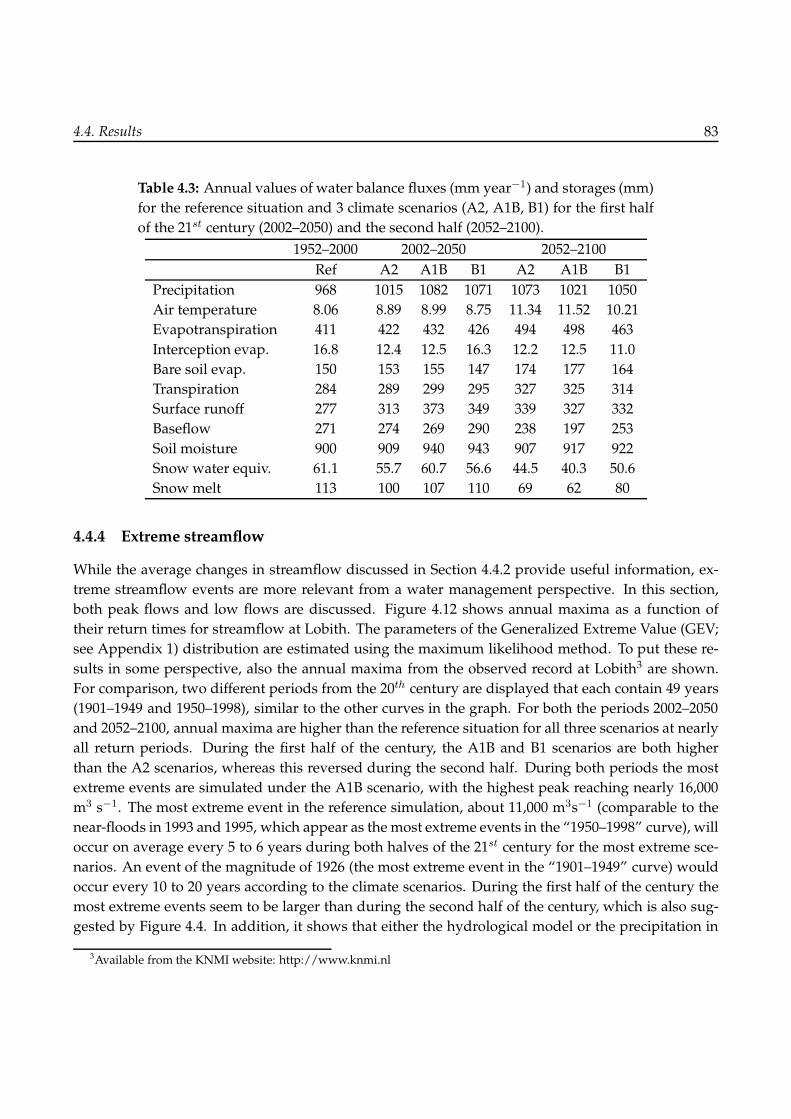
4.4. Results 83
Table 4.3: Annual values of water balance fluxes (mm year−1) and storages (mm)
for the reference situation and 3 climate scenarios (A2, A1B, B1) for the first half
of the 21st century (2002–2050) and the second half (2052–2100).
1952–2000 2002–2050 2052–2100
Ref A2 A1B B1 A2 A1B B1
Precipitation 968 1015 1082 1071 1073 1021 1050
Air temperature 8.06 8.89 8.99 8.75 11.34 11.52 10.21
Evapotranspiration 411 422 432 426 494 498 463
Interception evap. 16.8 12.4 12.5 16.3 12.2 12.5 11.0
Bare soil evap. 150 153 155 147 174 177 164
Transpiration 284 289 299 295 327 325 314
Surface runoff 277 313 373 349 339 327 332
Baseflow 271 274 269 290 238 197 253
Soil moisture 900 909 940 943 907 917 922
Snow water equiv. 61.1 55.7 60.7 56.6 44.5 40.3 50.6
Snow melt 113 100 107 110 69 62 80
4.4.4 Extreme streamflow
While the average changes in streamflow discussed in Section 4.4.2 provide useful information, ex-
treme streamflow events are more relevant from a water management perspective. In this section,
both peak flows and low flows are discussed. Figure 4.12 shows annual maxima as a function of
their return times for streamflow at Lobith. The parameters of the Generalized Extreme Value (GEV;
see Appendix 1) distribution are estimated using the maximum likelihood method. To put these re-
sults in some perspective, also the annual maxima from the observed record at Lobith3 are shown.
For comparison, two different periods from the 20th century are displayed that each contain 49 years
(1901–1949 and 1950–1998), similar to the other curves in the graph. For both the periods 2002–2050
and 2052–2100, annual maxima are higher than the reference situation for all three scenarios at nearly
all return periods. During the first half of the century, the A1B and B1 scenarios are both higher
than the A2 scenarios, whereas this reversed during the second half. During both periods the most
extreme events are simulated under the A1B scenario, with the highest peak reaching nearly 16,000
m3 s−1. The most extreme event in the reference simulation, about 11,000 m3s−1 (comparable to the
near-floods in 1993 and 1995, which appear as the most extreme events in the “1950–1998” curve), will
occur on average every 5 to 6 years during both halves of the 21st century for the most extreme sce-
narios. An event of the magnitude of 1926 (the most extreme event in the “1901–1949” curve) would
occur every 10 to 20 years according to the climate scenarios. During the first half of the century the
most extreme events seem to be larger than during the second half of the century, which is also sug-
gested by Figure 4.4. In addition, it shows that either the hydrological model or the precipitation in
3Available from the KNMI website: http://www.knmi.nl
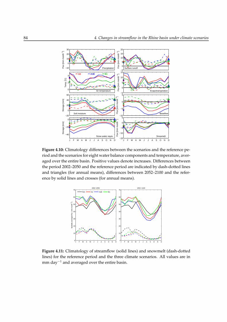
84 4. Changes in streamflow in the Rhine basin under climate scenarios
−10
0
10
20
30
Flu
x [m
m m
onth
−1 ]
Precipitation
0
2
4
Tem
p. [° C
]
Air temperature
A2 A1B B1
−20
0
20
40
60
Sto
rage
[mm
]
Soil moisture
J F M A M J J A S O N D
−40
−20
0
Sto
rage
[mm
]
Snow water equiv.
−5
0
5
10
15
20
Flu
x [m
m m
onth
−1 ]
Surface runoff
−5
0
5
10
15
Flu
x [m
m m
onth
−1 ]
Evapotranspiration
−10
−5
0
5
Flu
x [m
m m
onth
−1 ]
Baseflow
J F M A M J J A S O N D−15
−10
−5
0
5F
lux
[mm
mon
th−
1 ]
Snowmelt
Figure 4.10: Climatology differences between the scenarios and the reference pe-
riod and the scenarios for eight water balance components and temperature, aver-
aged over the entire basin. Positive values denote increases. Differences between
the period 2002–2050 and the reference period are indicated by dash-dotted lines
and triangles (for annual means), differences between 2052–2100 and the refer-
ence by solid lines and crosses (for annual means).
J F M A M J J A S O N D0
10
20
30
40
50
60
70
Spa
tially
ave
rage
d flu
x [m
m m
onth
−1 ]
2002−2050
Ref. A2 A1B B1
J F M A M J J A S O N D0
10
20
30
40
50
60
702052−2100
Figure 4.11: Climatology of streamflow (solid lines) and snowmelt (dash-dotted
lines) for the reference period and the three climate scenarios. All values are in
mm day−1 and averaged over the entire basin.

4.4. Results 85
1 5 10 20 50 1000
2000
4000
6000
8000
10000
12000
14000
16000
Dis
char
ge [m
3 s−
1 ]
2002 − 2050
Return period [years]1 5 10 20 50 100
2052−2100
Return period [years]
Reference
1901−−1949
1950−−1998
A2 scenario
A1B scenario
B1 scenario
Figure 4.12: Annualmaximum discharge at Lobith versus its return period for the
reference period (1952-2000) and three climate scenarios. Both the periods 2002–
2050 (left) and 2052–2100 (right) are displayed. A Generalized Extreme Value
(GEV)-distribution is adjusted to the data. In addition, two periods of 49 years
from the observed record are shown (1901–1949 and 1950–1998).
the reference dataset structurally overestimates events with low to medium return periods. For the
extreme events, models and observations agree well.
A similar analysis is carried out for streamflow droughts. Several approaches exist to define a drought
(e.g. Tallaksen and van Lanen, 2004; Fleig et al., 2006; Smakthin, 2001). Because not all annual low flow
events reflect a drought, we define a streamflow drought as a cumulative deficit of streamflow below
a threshold. At the moment the threshold is exceeded, the event ends (Hisdal et al., 2004). The thresh-
old was selected to be the 75th percentile of streamflow (meaning the streamflow that is equaled or
exceeded for 75% of the time) during the reference period (Hisdal et al., 2004). This value is a compro-
mise between the number of years without any events and the number of multi-year events, which
both can affect the results of the analysis (Fleig et al., 2006). Figure 4.13 shows the annual maximum
deficit volume of such events, versus their return periods. A Generalized Pareto (GP; see Appendix
1) distribution is a suitable distribution to model such cumulative deficits (Tallaksen et al., 2004; Fleig
et al., 2006). Therefore, such a distribution is adjusted to the data in Figure 4.13, again using maximum
likelihood estimation. Additional streamflow drought statistics are shown in Table 4.4. Here, three
statistics are selected: the average number of events per year, the average annual maximum duration,
and the average annual maximum intensity. The intensity is defined as the deficit volume (of which
the annual maxima are plotted in Figure 4.13), divided by the duration in seconds. The intensity
(shown in m3 s−1) can thus be seen as the average streamflow deficit during the event.
Figure 4.13 shows that during the first half of the century, streamflow drought deficits are lower than
the reference in all scenarios for small return periods. There are, however, some extreme events that

86 4. Changes in streamflow in the Rhine basin under climate scenarios
1 5 10 20 50 1000
20
40
60
80
100
120
140
Dis
char
ge d
efic
it [1
08 m3 ]
2002 − 2050
Return period [years]1 5 10 20 50 100
0
20
40
60
80
100
120
1402052−2100
Return period [years]
Reference
A2 scenario
A1B scenario
B1 scenario
Figure 4.13: Annual maximum cumulative deficit of streamflow with respect
to a threshold versus its return period for the reference period (1952-2000) and
three climate scenarios. The periods 2002–2050 (left) and 2052–2100 (right) are
displayed. The threshold is selected to be the 75th percentile at Lobith. A Gener-
alized Pareto (GP) distribution is adjusted to the data.
are considerably higher than the extreme events during the reference period, especially in the A2 sce-
nario. For the second half of the century the picture is entirely different: for nearly all return periods
and all three scenarios streamflow drought deficits are larger than in the reference simulation. The
most extreme streamflow drought deficit in the reference simulation, about 40×108 m3, occurs every 3
to 10 years depending on the scenario. The most extreme events during the period 2052–2100 occur in
the A1B scenario and have a drought deficit volume that is more than double the volume during the
reference period. Table 4.4 shows the streamflow drought events events in more detail. Because statis-
tics are shown for different locations in the basin (Figure 1.5), it also shows which regions are most
susceptible to streamflow droughts. In Table 4.4, it can be seen that there are indeed significant re-
gional differences within the basin. While the overall trend confirms the trends shown in Figure 4.13,
there are some exceptions. For example, in the Mosel catchment, number, duration and intensity all
keep decreasing during the 21st century. This seems in contradiction with Figure 4.6. Here it can be
seen that a large part of the Mosel catchment experiences a decrease in summer evapotranspiration,
supposedly due to water limitation. In winter however, there is also an increase in precipitation. An
explanation for this contradiction is the fact that the winter precipitation rapidly percolates to the
groundwater, where the water is out of reach for plants. Soil moisture droughts thus occur because
evapotranspiration is water limited. However, the groundwater sustains relatively high baseflow lev-
els, preventing streamflow droughts to occur (Tallaksen and van Lanen, 2004).
From Table 4.4, the Neckar basin appears to be the most susceptible to streamflow droughts: espe-
cially for the A1B scenario the average maximum duration increases from 29 to 81 days (the overall
highest value), and the intensity rises from 29 to 60 m3s−1, which is also the highest value relative

4.5. Discussion 87
to the threshold streamflow (which is only 108 m3s−1). The A1B scenario shows the highest val-
ues of drought statistics for most sub-basins and the entire basin, which corresponds to Figure 4.13.
Figures 4.5 and 4.6 explain the fact that the Neckar sub-basin appears to be extremely vulnerable to
streamflow drought events through the combination of strongly decreasing summer precipitation,
only weakly increasing winter precipitation and increasing summer evapotranspiration. The same
holds for the Alpine area, represented by Maxau. Because a large part of the Rhine discharge origi-
nates upstream of Maxau, this also has a strong influence at Lobith, the basin outlet.
4.5 Discussion
In this study we have investigated the effect of climate change on streamflow dynamics in the Rhine
basin, by means of downscaled regional climate scenarios (0.088◦ spatial resolution) and a hydrolog-
ical model. To represent the current climate two atmospheric datasets were available: a validation
dataset based on re-analysis data that was used to calibrate the hydrological model, and a reference
dataset based on a model run for the period 1050–2000 that was used for comparison with the scenar-
ios. For each dataset, a bias correction was carried out to account for structural model errors. Three
scenarios were available according to three SRES-emission scenarios: A2, A1B and B1. As a macro-
scale hydrological model, the Variable Infiltration Capacity model was used, which is a land-surface
model that has been applied in hydrological applications before. Changes in average streamflowwere
investigated, as well as changes in peak flow and streamflow droughts for different locations in the
basin.
Data from a single GCM, RCM and hydrological model were used, whereas ideally one would use
an ensemble for each model type. Model comparisons indicate a large range in model projections be-
tween GCMs. For example, the Coupled Model Inter comparison Project (CMIP) compared globally
averaged air temperatures for the period 1961-1990s simulated by 18 GCMs and found a range ofmore
than 4◦C around the observed 14◦C (Covey et al., 2003). For precipitation, a similar range was found.
Also the projected trend in global temperature structurally differs between GCMs. For example, the
GCM used in this study, ECHAM5-OM, is known to give relatively strong temperature increases in
the second half of the 21st century. As a model comparison in IPCC (2007) shows, ECHAM is rela-
tively “cool” compared to themulti-model mean in the first half of the century, and relatively warm in
the second half. The reason is a relatively high sensitivity of ECHAM to aerosol concentrations: in the
first half of the century aerosol concentrations are high and their dimming effect is relatively strong.
In the second half of the century, the model reacts strongly to the decline of aerosol concentrations,
causing a strong temperature increase. This feature partly explains the contrast in our results between
the periods 2001–2050 and 2051–2100 (relatively wet versus relatively dry), and further illustrates the
need for a similar analysis with an ensemble of GCMs. The fact that in CMIP the ECHAM4-model
is quite close to observed values for global mean temperature and precipitation (Figure 1 of Covey
et al. (2003)), is encouraging. Also in model comparisons regarding other climate variables, ECHAM

88 4. Changes in streamflow in the Rhine basin under climate scenarios
Table 4.4: Statistics of streamflow drought events during the reference period
and the 1st and 2nd half of the 21st century for the three climate scenarios (A2,
A1B and B1), for seven streamflow gauges in the Rhine basin. For locations and
corresponding sub-basins see Figure 1.5. Three statistics are shown, indicated by
S1, S2 and S3. S1 is the average number of events (i.e., non-exceedence of the
threshold) per year. S2 is the average of annual maximum durations in days.
S3 is the average of annual maximum intensities, where the intensity is defined
as deficit volume (plotted in Figure 4.13) divided by duration, in m3 s−1. For
each station, the threshold value (75th percentile of the reference period) is shown
between parentheses.
Reference A2 scenario A1B scenario B1 scenario
Period S1 S2 S3 S1 S2 S3 S1 S2 S3 S1 S2 S3
Hattingen (37.8 m3s−1)
2002–20505.7 33 16.8
6.5 33 17.6 5.0 27 15.6 4.6 26 12.9
2052–2100 7.1 35 19.7 6.7 39 19.9 6.0 33 18.9
Kalkofen (17.0 m3s−1)
2002–20507.5 33 5.6
8.1 30 5.8 7.3 25 5.5 6.0 22 4.6
2052–2100 8.7 32 7.1 9.0 34 7.1 7.3 28 6.2
Raunheim (92.9 m3s−1)
2002–20506.5 34 22.5
5.4 31 17.7 5.0 25 16.5 4.0 23 14.7
2052–2100 6.2 37 19.2 5.7 40 17.8 6.0 35 17.3
Cochem (165.9 m3s−1)
2002–20506.4 37 37.9
6.1 32 32.1 6.1 40 38.8 5.9 26 33.5
2052–2100 4.2 34 24.3 3.9 35 22.1 4.0 23 20.4
Rockenau (107.8 m3s−1)
2002–20507.0 29 29.1
5.5 26 23.5 7.4 25 27.2 4.1 24 21.6
2052–2100 9.5 44 40.0 11.8 81 60.1 8.4 42 36.8
Maxau (986.9 m3s−1)
2002–20504.8 33 209
4.1 30 217 4.1 20 204 4.1 23 173
2052–2100 7.2 33 334 8.7 38 420 5.8 28 259
Lobith (1801 m3s−1)
2002–20506.8 32 475
5.8 27 424 5.4 21 400 5.0 21 363
2052–2100 7.7 38 614 8.8 46 722 6.7 33 510
is ranked among the best performing GCMs (van Ulden and van Oldenborgh, 2006). In a recent model
comparison, Reichler and Kim (2008) showed that ECHAM5-OM (which we use) performs very well
compared to most other GCMs in simulating the current climate in terms of many different climate
variables. The range of temperature changes that is projected by GCMs is further extended by the
RCMs that are used for downscaling (e.g. van den Hurk et al., 2005; Jacob et al., 2007; Deque et al., 2007).

4.5. Discussion 89
In addition to the uncertainty in atmospheric models, there is also uncertainty involved in hydrolog-
ical models and their parameterizations. However, given the fact that each GCM and RCM requires
a specific bias correction (associated with different structural model errors), and each combination
of a hydrological model with an atmospheric dataset would require a specific calibration, it was not
feasible in the present study to use multiple models.
The bias correction that was applied to the meteorological data altered the spatial pattern of pre-
cipitation and temperature because the correction was applied to each of 134 sub-basins for which
observations were available. As was noted in Section 4.4.1 and can be seen in Figure 4.3, the spa-
tial pattern from the RCM is “drawn” towards that of the observations. In addition, the difference
between the reference dataset and the scenarios can be amplified or reduced somewhat because the
same exponent (Eq. 4.1) is applied to both. When the basin-wide spatial average is considered, this
effect largely cancels out. This feature, however, is inherent to our correction for the model bias,
which can be seasonally and geographically varying (e.g Christensen et al., 2008; Leander and Buishand,
2007). The above should be kept in mind when interpreting the spatial patterns as presented in this
paper, or comparing them with uncorrected climate scenarios. Furthermore, while we assume that
the model biases are similar for the current climate and the changing climate, Christensen et al. (2008)
found that this is not always valid and biases tend to grow under warming conditions and depend on
the amount of precipitation. This suggests an overestimation of the temperature increase, and should
be kept in mind when interpreting the results.
The hydrological model that we used also presents some issues for discussion. While the VIC model
has a physically- based approach for the calculation of evapotranspiration by solving the coupled
water and energy balance, this is not the case for subsurface hydrological processes. No lateral soil
moisture movement is included and the contribution of groundwater to evapotranspiration by cap-
illary uprise is neglected as well. For an accurate modeling of streamflow drought events, ideally an
explicit groundwater model should be included. However, at the scale of a large river basin, such as
the Rhine, this is numerically not feasible. There has been some recent progress in including ground-
water processes in land surface models like VIC (e.g. Maxwell and Kollet, 2008), although only for
applications to small catchments. Because in the present study drought characteristics are not com-
pared with observations but with a reference simulation, the presented results do provide valuable
information on relative changes in drought characteristics as caused by climate change.
Finally, it is important to mention that the presented analysis of hydrological extremes is based on
relatively short time series (3 x 100 years), whereas the Rhine discharge at Lobith that is relevant for
safety purposes has a return period of 1250 years (de Wit and Buishand, 2007). The highest occurring
streamflow in this study (about 16,000 m3s−1) is associated with much shorter return periods and
therefore does not imply that higher values are not possible. Moreover, in this study river hydraulics
and floodings are not taken into account, whereas floodings in Germany would have a significant
impact on peak discharge at Lobith (de Wit and Buishand, 2007).

90 4. Changes in streamflow in the Rhine basin under climate scenarios
4.6 Conclusions
The present study differs from previous climate change impact assessments in the Rhine basin re-
garding the following points: the spatial resolution of the employed climate scenarios is higher; the
hydrological model is more physically based and the entire 21st century was investigated as opposed
to a timeslice of typically 30 years.
As far as streamflow at Lobith is concerned, this study confirms previous climate change impact as-
sessments in the Rhine basin. By the end of the century, average streamflow at basin outlet is projected
to increase with about 30% in winter and spring and to decrease with a similar value in summer and
autumn. The majority of this effect originates in the alpine part of the catchment. It is caused for a
large part by a decrease of the contribution of snowmelt to streamflow and by a shift of the timing of
the snowmelt season to earlier in the year.
The high-resolution climate scenarios and the (distributed) hydrological model allow for a detailed
analyses of spatial patterns. Results indicate that the projected decrease in summer discharge is con-
centrated in the southern part of the basin. The northern tributaries, where there is hardly any de-
crease in summer precipitation, are dominated by wetter conditions throughout the year.
The availability of data for the entire century allows the analysis of trends throughout the century,
of which an overview is displayed in Figure 4.4. Towards the end of the 21st century, a gradually
decreasing trend in annual maximum, minimum and mean streamflow appears. This trend causes
an interesting contrast between the first half and the second half of the century. Because precipitation
significantly increases in all three scenarios, the first half is dominated by relatively wet conditions.
This also shows in our analysis of peak flows. During the second half of the century, temperature
and evapotranspiration increase more drastically than during the first half, causing generally dryer
conditions and more extreme droughts. Partly, this contrast originates from our choice of the GCM
(see Section 4.5). It would be very interesting to repeat this analysis with another, or multiple, GCMs.
Acknowledgements
This research was financially supported by the European Commission through the FP6 Integrated
Project NeWater and the BSIK ACER project of the Dutch Climate Changes Spatial Planning Pro-
gramme. Rita Lammersen and Hendrik Buiteveld from Rijkswaterstaat Waterdienst, The Nether-
lands, are kindly acknowledged for providing observed data.

Chapter 5
Effects of climate variability on water storage in the Colorado River Basin
This chapter is a modified version of: R. T. W. L. Hurkmans, P. A. Troch, R. Uijlenhoet, P. J. J. F. Torfs and M.
Durcik (2009), “Effects of climate variability on water storage in the Colorado basin,”, submitted to J. Hydrometeorol.

92 5. Effects of climate variability on water storage in the Colorado River Basin
Abstract
Understanding the long-term (interannual to decadal) variability of water availability in river basins is
paramount for water resources management. Here, we analyze time series of simulated terrestrial water
storage components, observed precipitation and discharge spanning 74 years in the Colorado River Basin
and relate them to climate indices that describe variability of sea surface temperature and sea level pressure
in the tropical and extra-tropical Pacific. El Nino-Southern Oscillation (ENSO) indices in winter (JFM) are
related to winter precipitation, as well as to soil moisture and discharge in the Lower Colorado. The low-
frequency mode of the Pacific Decadal Oscillation (PDO) appears to be strongly correlated with deep soil
moisture. During the negative PDO phase, saturated storage anomalies tend to be negative, and the “ampli-
tudes” (mean absolute anomalies) of shallow soil moisture, snow and discharge are slightly lower compared
with periods of positive PDO phases. Predicting interannual variability, therefore, strongly depends on the
capability of predicting PDO regime shifts. If indeed a shift to a cool PDO phase occurred in the mid-nineties,
as data suggest, the current dry conditions in the Colorado basin may persist.

5.1. Introduction 93
5.1 Introduction
Recently, the Colorado River Basin (CRB) experienced a severe multi-year drought that is unprece-
dented in the hydroclimatic record (Cook et al., 2004). Due to temperature rise associated with climate
change, similar drought episodes are predicted to occur more often (Seager et al., 2007). For water
management operations in the basin, understanding and predictive capacity of terrestrial water stor-
age (TWS) dynamics and its associated hydrologic fluxes is crucial (Troch et al., 2007). Precipitation
in the southwestern U.S. has been linked to oceanic interannual variability (e.g. Redmond and Koch,
1991; Okin and Reheis, 2002; McCabe et al., 2004; Hidalgo and Dracup, 2003), mostly involving El Nino-
Southern Oscillation (ENSO; Trenberth (1997b)) and Pacific Decadal Oscillation (PDO; Mantua et al.
(1997), a special case of Pacific Decadal Variability (PDV)). ENSO is considered the most important
process of interannual variability of water availability in the southwestern U.S., and the most reliable
one in terms of prediction (Cayan et al., 1999). Warm (El Nino) and cold (La Nina) events typically oc-
cur every 3 to 7 years and last 8 to 16 months. These events have been linked to precipitation, floods
and droughts across the western-United states (Cayan et al., 1999; Canon et al., 2007; Hamlet et al., 2007).
La Nina conditions lead to wet conditions in the Northwest and dry conditions in the Southwest, and
vice versa for El Nino conditions (Redmond and Koch, 1991). PDO shows similar effects in the south-
western U.S. (MacDonald and Case, 2005) and can, when in phase with ENSO, amplify El Nino or La
Nina effects (Gershunov and Barnett, 1998; Hamlet et al., 2007; Cole et al., 2002). PDO regime shifts,
however, are much less predictable than ENSO cycles. Although its power spectrum was shown to
be most energetic at two ranges of return periods (one from 15-25 years and the other 50-70 years;
Mantua and Hare (2002)), the physical processes driving PDV and PDO remain unclear. The abrupt
changes between cool and warm phases (each lasting 20-30 years), therefore, are not yet predictable
with sufficient lead times (Newman, 2007).
Much of previous research has focused on precipitation and, to a lesser degree, on streamflow (e.g.,
Maity and Kumar, 2008). Much less attention has been paid to regional water availability or terrestrial
water storage (TWS; Troch et al. (2007)). Understanding the effects of climate variability on TWS is,
however, relevant, since it is a hydrologic state variable and therefore integrates hydrologic processes
such as snow accumulation, evapotranspiration, infiltration and recharge. There are several tech-
niques available to estimate TWS, which are described in detail in Troch et al. (2007). Examples are the
Basin-scale Water Balance (BSWB) method, used by Seneviratne et al. (2004) and Hirschi et al. (2006),
which combines the atmospheric and terrestrial water balance to estimate changes in TWS from at-
mospheric moisture convergence, changes in atmospheric water vapor storage, and streamflow data.
The GRACE satellite mission (Tapley et al., 2004), has been also applied successfully to estimate water
storage variability (e.g. Swenson andMilly, 2006; Han et al., 2005). A third method is hydrological mod-
eling of TWS-components. Among all these methods, estimated storage dynamics in the CRB agree
reasonably well with each other and with in-situ data (Troch et al., 2007; Hasan et al., in prep.).
Here, we focus on TWS dynamics simulated using the Variable Infiltration Capacity hydrological

94 5. Effects of climate variability on water storage in the Colorado River Basin
model (VIC; Liang et al. (1994)) forced by a meteorological dataset of interpolated observations, span-
ning the period 1915–2003. Hydrological modeling has several advantages compared to the other
methods mentioned above. First, simulations are based on observedmeteorological forcings (precipi-
tation, temperature, air pressure, short- and longwave incoming radiation, vapor pressure, and wind
speed), whereas for example the BSWBmethod applies model re-analysis data, which are constrained
by radiosonde observations. Especially for hydrologic variables, balance problems can occur in such
datasets (Seneviratne et al., 2004). Second, TWS estimates from VIC span a longer period (1915-2003)
compared to the other methods. Third, TWS can be investigated in a distributed manner. Finally,
TWS can be analyzed for each of its components (such as soil moisture, snow, groundwater) sepa-
rately. Troch et al. (2007) and Hasan et al. (in prep.) indicated that the amplitudes of modeled storage
anomalies do not always agree well with that of other methods, and Niu and Yang (2006) found that
they are generally too low in tropical regions and too high at high latitudes. Trends and variability,
however, agree well (see also: http://voda.hwr.arizona.edu/twsc/sahra/, 2008).
We analyze the interannual variability of individual components of TWS: shallow and deep soil mois-
ture, and snow water equivalent (SWE), as well as precipitation and discharge. Using several climate
indices describing oceanic and atmospheric variability in the Pacific, we attempt to explain this vari-
ability. With enhanced understanding of this variability, predictability of hydrologic anomalies in the
CRB may be improved. As already mentioned, an advantage of obtaining TWS from hydrological
modeling, is its relatively high spatial resolution. Storage dynamics will, therefore, be analyzed both
in a spatially averaged and a distributed way.
5.2 Study area and datasets
The Colorado River Basin (CRB) is located in the southwesternUnited States, and has a drainage area
of about 637,000km2 (Figure 5.1). Much of the basin is semi-arid, and in the southern part rainfall is
generally concentrated in the summer monsoon. The high-elevation snow pack in the Rocky Moun-
tains contributes about 70% of the total annual runoff.
The meteorological data used in this study were compiled by Hamlet and Lettenmaier (2005) and span
the period from 1915 to 2005. Based on comparisons with observed streamflow and snow cover,Ham-
let and Lettenmaier (2005) concluded that the dataset is temporally consistent and suitable for trend
analysis of hydrologic variables at the macro-scale. The Hamlet and Lettenmaier (2005) dataset is thus
used to force the Variable Infiltration Capacity (VIC, version 4.0.5; Liang et al. (1994)) model for the
CRB at a spatial resolution of 0.25◦ and a temporal resolution of 3 hours. The VIC model is designed
as a land surface model to provide the land surface boundary conditions for climate models. Evapora-
tion is calculated by solving the coupledwater and energy balance, and the soil column is represented
by three layers. The soil moisture contents of the upper two, of which the upper is generally very thin
(0.1m), determine the amounts of evaporation and infiltration. The soil moisture content of the lowest

5.2. Study area and datasets 95
Figure 5.1: Location of and elevations in the Colorado River Basin. The basin
outline represents the discretization of the basin in VIC at a resolution of 0.25
degrees. The Colorado river is shown as a black line.
layer determines the amount of baseflow, or groundwater discharge. Vertical transport of moisture
through the soil column is assumed to be driven by gravity only and no lateral moisture transport is
allowed. Calibration parameter values for the VIC model were obtained from A.Wood (University of
Washington; personal communication). The model was calibrated to match naturalized streamflow
at the basin outlet. Resulting modeling efficiencies at the outlet of the Upper Colorado and the entire
CRB were respectively 0.88 and 0.85, where a value of 1 indicates a perfect match. From the modeling
results the following variables were extracted: outflow (surface runoff plus baseflow), snow water
equivalent (SWE), soil moisture in the lowest layer (hereafter denoted as deep soil moisture) and soil
moisture in the upper two layers (hereafter denoted as shallow soil moisture). The latter three, as well
as interception storage of the canopy (both snow and water), are summed to calculate total TWS. In
addition, precipitation from the forcing dataset is included in the analyses. Due to the dominance of
the summer monsoon and spring snowmelt, all variables show a very strong annual cycle compared
to the interannual variability. To remove seasonal influences, and because all climate indices are also
based on a monthly time step, all time series are aggregated to monthly averages (sums for precipita-
tion and outflow) and converted to anomalies by subtracting the mean annual cycle. Smoothed time
series (12 month running means) of all anomalies are shown in Figure 5.2a and b, their autocorrelation
functions are shown in Figure 5.3a and the corresponding power spectrum in Figure 5.3b. Because
storage anomalies in the first 15 years were very high compared to the rest of the period, while pre-
cipitation anomalies were not, we discarded the first 15 years. The period of analysis is, therefore,
1930–2003 hereafter.
Precipitation over the CRB has been linked to both tropical (ENSO) and extratropical (PDO) Pacific

96 5. Effects of climate variability on water storage in the Colorado River Basin
−18
−12
−6
0
6
12
18
Sto
rage
com
pone
nts
[mm
]
a) −36
−24
−12
0
12
24
36
Tot
al s
tora
ge [m
m]
Shallow soil moist. Deep soil moist. SWE TWS
−2.5−2
−1.5−1
−0.50
0.51
1.52
2.5
b)
Dra
inag
e [m
m m
onth
−1 ]
−12.5−10−7.5−5−2.502.557.51012.5
Pre
cipi
tatio
n [m
m m
onth
−1 ]
Outflow Precipitation
1930 1940 1950 1960 1970 1980 1990 2000
−2
−1
0
1
2
Inde
x [−
]
c)
PDO NINO34 MEI PNA
Figure 5.2: Time series of spatially averaged anomalies of (a) storage components
and total storage in VIC, (b) outflow (surface runoff + baseflow) and precipitation,
and (c) four climate indices (MEI, PDO, NINO3.4 and PNA). For clarity, 12 month
running averages were calculated for each variable.
variability. Therefore, four indices that together represent both oceanic and atmospheric dynamics
in the tropical and extratropical Pacific were selected. The Multivariate Enso Index (MEI; Wolter and
Timlin (1998)) was selected because it is a composite of six variables over the tropical Pacific, and
includes atmospheric anomalies in addition to sea surface temperatures (SST). Because MEI is only
available from 1950, we use NINO3.4 (which is available for the entire period) as a proxy because it
shows the highest correlation with MEI (0.90) compared with other ENSO indices (NINO1.2, NINO3
and NINO4). The difference between these ENSO indices is the area in the Pacific that is used to cal-
culate them. NINO3.4 is calculated over the area bounded by 5◦N–5◦S in latitude, and 170◦W–120◦W
in longitude. For NINO3 and NINO4, these bounding boxes have the same latitudes, but in longitude
the ranges are 150◦W–90◦W for NINO3 and 160◦E–150◦W for NINO4. NINO1.2 is bounded by 0◦–
10◦S latitude, and 90◦W–80◦W longitude. To represent PDO, the PDO index proposed byMantua et al.
(1997) is used, defined as the anomaly of sea surface temperature in the area of the Pacific north of
20◦N. In addition, the Pacific North American pattern (PNA) is included because it is one of the most
important modes of variability in the Northern Hemisphere extratropical atmosphere, and largely in-
dependent of ocean temperatures (Johansson, 2007). In addition, PNAwas shown to have an influence
on precipitation and discharge in the western United States by Redmond and Koch (1991). In this way

5.2. Study area and datasets 97
we cover both ocean and atmospheric dynamics in the tropics (MEI/NINO3.4) and the extratropics
(PDO/PNA). Figure 5.2c shows 12-month running mean time series of all four indices and Figure 5.3b
shows their autocorrelation functions (ACFs) and power spectra respectively. MEI and NINO3.4 have
their most important spectral peaks at return periods of about 4 to 6 years, whereas PDO shares the
peak at 6 years with ENSO, but has its most important peaks at 25 years and higher. However, the
time series that is employed is too short (74 years) to capture this low-frequency behavior of PDO.
Cross-correlations and cross-powerspectra between anomalies and climate indices were analyzed as
well. Because in many signals there is significant autocorrelation (Figure 5.3a,c), they were found to
provide little information and are therefore not shown in this article.
−0.2
0
0.2
0.4
0.6
0.8
Cor
rela
tion
coef
ficie
nt [−
]
a)
Shallow soil moist.Deep soil moist.SWETWS
0 0.2 0.4 0.6 0.810
20
30
40
50
60
70
80
Pow
er [d
B]
b)
DischargePrecip.
0 24 48 72 96 120 144 168−0.4
−0.2
0
0.2
0.4
0.6
0.8
1
Time lag [months]
Cor
rela
tion
coef
ficie
nt [−
]
c)
NINO3.4PDOMEIPNA
0 0.2 0.4 0.6 0.80
10
20
30
40
50465
74625
Frequency [year−1]
Pow
er [d
B]
d)
Figure 5.3: Autocorrelation functions for all anomalies (a) and indices (c) dis-
played in Figure 5.2, up to a time lag of 180 months (15 years). Gray shaded areas
indicate autocorrelations not significantly different from zero. Power spectra are
also shown for anomalies (b) and climate indices (d). Numbers in d) represent
the return period in years of the strongest spectral peaks of NINO3.4 and PDO.
Both (a) and (b) show six lines (shallow soil moisture, deep soil moisture, SWE,
TWS, discharge, and precipitation) for which the legend is split between (a) and
(b).
98 5. Effects of climate variability on water storage in the Colorado River Basin
5.3 Results
5.3.1 Analysis of spatial averages
As can be seen in Figure 5.3, the autocorrelation function for deep soil moisture remains significant
for very large time lags, up to about 11 years. The large autocorrelation propagates in the total TWS,
causing the autocorrelation function for total TWS to be significant up to about 6 years, although small
after 1 year. Therefore, in the analyses described hereafter, dynamics of total TWS are not examined
as such, but storage dynamics for deep soil moisture, shallow soil moisture and SWE are investigated
separately. For these latter variables, the autocorrelation function diminishes after a few months, so
by calculating averages of 6 months, autocorrelation is almost filtered out and correlation patterns
between climate indices and anomalies can be investigated, including time lags. Figure 5.4 shows a
matrix of correlation coefficients between monthly values of the climate indices and 6 month moving
averages of anomalies of shallow soil moisture, SWE, discharge and precipitation.
In Figure 5.4, correlation patterns are similar for precipitation, shallow soil moisture and discharge,
although correlation coefficients are generally slightly lower for discharge. MEI and NINO3.4 show
a nearly identical pattern, which is not surprising given their high mutual correlation (0.90). ENSO
indices early in the year (January to May) give the highest correlations with hydrologic anomalies
throughout the year, except for the period which is dominated by the summer monsoon. This is con-
sistent with the findings of, for example, Okin and Reheis (2002) and Gochis et al. (2007), who found
low correlations between winter ENSO and summer precipitation as well. ENSO indices in the sec-
ond half of the year, on the other hand, seem to be correlated with the second half of the year (the
monsoon and the period just after that). These findings are consistent with previously reported corre-
lations. Hidalgo and Dracup (2003) report high correlations of warm season ENSO with warm season
precipitation in the upper Colorado basin, whereas in the lower Colorado basin correlations are gen-
erally found to be higher between winter ENSO and winter precipitation (e.g. Okin and Reheis, 2002).
PDO shows a slightly different pattern, with significant correlations for all but the winter months and
generally slightly lower correlations. The amount of snow in the winter season, however, seems to
be uncorrelated to any climate index. There is some correlation between SWE and MEI in summer,
but that is only after the main snow melt season, when there is hardly any snow left. The lack of
correlation between SWE and ENSO is consistent with the result that correlations between ENSO and
winter precipitation are limited to the Lower Colorado basin, since SWE is concentrated in the Upper
Colorado basin. The PNA index in some specific months (January and April) is also correlated with
SWE, especially in the cold season. It should be noted, however, that due to limited availability of the
climate indices, MEI and PNA only cover the period 1950-2003, while NINO3.4 and PDO cover the
entire period from 1930.
By calculating the 6-month averages, the effect of autocorrelation should be filtered out. To further
investigate the correlations that appear in Figure 5.4, the corresponding (scaled) time series to some of
the pixels in Figure 5.4 are shown in Figure 5.5. Here, only PDO andNINO3.4 are shown because they

5.3. Results 99
Index month #
Per
iod
of a
nom
aly
Shallow moist.−PNA
JFMAMJ JASOND
D−MO−MA−JJ−NA−SF−J
Index month #
SWE−PNA
JFMAMJ JASONDIndex month #
Discharge−PNA
JFMAMJ JASONDIndex month #
Precipiatation−PNA
JFMAMJ JASOND
−0.5 −0.4 −0.3 −0.2 −0.1 0 0.1 0.2 0.3 0.4 0.5
Index month #
Snow + moist.−PNA
JFMAMJ JASOND
Per
iod
of a
nom
aly
Shallow moist.−MEI
D−MO−MA−JJ−NA−SF−J
SWE−MEI Discharge−MEI Precipiatation−MEI Snow + moist.−MEI
Per
iod
of a
nom
aly
Shallow moist.−PDO
D−MO−MA−JJ−NA−SF−J
SWE−PDO Discharge−PDO Precipiatation−PDO Snow + moist.−PDO
Per
iod
of a
nom
aly
Shallow moist.−NINO34
D−MO−MA−JJ−NA−SF−J
SWE−NINO34 Discharge−NINO34 Precipiatation−NINO34Snow + moist.−NINO34
Figure 5.4: Correlation between 6-month moving averages of 5 hydrologic
anomalies and monthly values of 4 climate indices (on the X-axes). The Y-axes,
thus, represent from bottom to top 12 six-month moving averages: January-June,
February-July (F-J)...December-May (D-M). Correlations that are significant at
α = 0.05 are denoted by a black dot.
cover the entire period, and only shallow soil moisture is shown because precipitation and discharge
show a similar correlation pattern in Figure 5.4. Figure 5.5 shows that both the NINO3.4 and PDO
indices are indeed related to anomalies of shallow soil moisture in winter and spring (Figure 5.5):
nearly all the El Nino (La Nina) events (shaded in gray) correspond to a positive (negative) shallow
soil moisture anomaly. Here, the definition of such events as given by Trenberth (1997b) is followed:
an event is a consecutive period of 6 months in which the NINO3.4 index is higher than 0.4◦C (for El
Nino), or lower than−0.4◦C (for La Nina). The same events are also visible for the PDO index, which
explains the nearly identical correlation coefficients for both indices. Climate indices in March are cor-
related to shallow soil moisture throughout the year (Figures 5.5a-d), whereas the climate indices in
September are only correlated with cold season shallow soil moisture (Figures 5.5g,h), and much less
(not at all for NINO3.4) with warm season shallow soil moisture (Figures 5.5e,f). In all plots, it appears
that especially the extreme El Nino and La Nina events are generally well correlated. For example,
the El Nino event of 1940, which also shows a high PDO peak, is related to high shallow soil moisture

100 5. Effects of climate variability on water storage in the Colorado River Basin
−0.5
0
0.5S
cale
d tim
eser
ies
[−]
ρNino34, SM
= 0.38
a) NINO34 Shallow moist.
−0.5
0
0.5
ρPDO, SM
= 0.37
b) PDO Shallow moist.
−0.5
0
0.5
ρNino34, SM
= 0.36
Sca
led
times
erie
s [−
]
c)
−0.5
0
0.5
ρPDO, SM
= 0.37
d)
−0.5
0
0.5
ρNino34, SM
= −0.01
Sca
led
times
erie
s [−
]
e)
−0.5
0
0.5
ρPDO, SM
= 0.27
f)
1930 1940 1950 1960 1970 1980 1990 2000
−0.5
0
0.5
ρNino34, SM
= 0.30
Sca
led
times
erie
s [−
]
g)
1930 1940 1950 1960 1970 1980 1990 2000
−0.5
0
0.5
ρPDO, SM
= 0.43
h)
Figure 5.5: Time series of monthly NINO3.4 (a,c,e,g), PDO (b,d,f,h) and 6-month
averaged shallow soil moisture, similar to the data used to create Figure 5.4. Four
pixels from the matrices plotted in Figure 5.4 are used: a/b) the March indices
versusMarch-September averaged shallow soil moisture; c/d)March indices ver-
sus September-February averaged shallow soil moisture; e/f) September indices
versus March-September averaged shallow soil moisture and g/h) September in-
dices versus September-February averaged shallow soil moisture. Also the cross-
correlation coefficients (without time lag) are shown in every panel (SM indicates
soil moisture). Gray shaded areas indicate El Nino events (positive) and La Nina
events (negative).
anomalies throughout the year. Also the El Nino events of around 1972 and 1982 and the La Nina
event of 1989 led to extremely wet (dry for La Nina) conditions. However, they were not so distinct
throughout the year, i.e. they do not show up in all panels of Figure 5.5. It should be noted, however,
that although Figure 5.5 shows the dynamics of climate indices and shallow soil moisture anomalies,
the amplitudes of all signals (also with respect to each other) have no meaning because all time series
were scaled by dividing each time series by the difference between its maximum andminimum value.
For some of the variables and indices in Figure 5.2, the 24-month running average is plotted in Fig-

5.3. Results 101
−1.5−1
−0.50
0.51
1.5C
limat
e in
dex
[−]
a)
−20
−10
0
10
20
Ano
mal
y [m
m]
−1.5−1
−0.50
0.51
1.5
Clim
ate
inde
x [−
]
b)
−6−4−202468
Ano
mal
y [m
m]
−1.5−1
−0.50
0.51
1.5
Clim
ate
inde
x [−
]
c)
0
Ano
mal
y [m
m]
−1.5−1
−0.50
0.51
1.5
Clim
ate
inde
x [−
]
d)
−10
−5
0
5
10
Ano
mal
y [m
m m
−1 ]
1930 1940 1950 1960 1970 1980 1990 2000
−1.5−1
−0.50
0.51
1.5
Clim
ate
inde
x [−
]
e)
0
Ano
mal
y [m
m m
−1 ]
Anomaly NINO34 PDO Lake Mead
Figure 5.6: Interannual variability investigated through time series of 24-month
running averages of a) deep soil moisture, b) shallow soil moisture, c) SWE, d)
precipitation and e) discharge. In all plots, also NINO3.4 and PDO are plotted.
In addition, the storage anomaly of Lake Mead is plotted in a). To illustrate the
correlation between deep soil moisture and reservoir storage and PDO phases,
the 10-year running means of the deep soil moisture anomaly (black) and that of
the storage anomaly of Lake Mead (gray) are plotted as well in a) as thick dashed
lines. Black vertical lines denote the shifts from warm to cool and again to warm
PDO phase in all panels, and the dashed line at 1998 denotes a possible third
phase change.
ure 5.6 in order to show interannual to decadal variability more clearly. The PDO phases, each about
30 years long, clearly stand out. PDO phases were identified by several independent studies (see
Mantua and Hare (2002) for a review on PDO) as follows: warm (positive) PDO regimes dominated
from 1925 to 1946 and from 1977 to about the mid-nineties, whereas cool (negative) regimes prevailed

102 5. Effects of climate variability on water storage in the Colorado River Basin
between 1947-1976. The 74 years used in this study, therefore, only cover one complete PDO cycle. In
Figure 5.6, regime shifts as they were indicated by Mantua et al. (1997) are indicated by vertical black
lines.
In Figure 5.6a the sign of the anomaly of deep soilmoisture is distinctly different between PDOphases.
This is illustrated by the 10-year running mean (dash-dotted line in Figure 5.6a), of which the posi-
tive and negative episodes exactly coincide with the PDO phases. Apparently, during negative PDO
episodes conditions are generally dryer, although this does not show that clearly in the other records.
In addition, the storage anomaly of Lake Mead is plotted in Figure 5.6a. Lake Mead is a large surface
water storage reservoir in the Lower Colorado, accounting for 45% of the total surface storage capac-
ity in the CRB (Troch et al., 2007), and data is available from 1941 onwards. Another large reservoir,
Lake Powell (accounting for 42% of the total storage capacity), is only operational from 1963 and is
therefore not included in the present analysis. The 24-month running average of the storage anomaly
of LakeMead follows the deep soil moisture anomaly with a time lag, although the signal is somewhat
flattened. In addition, the 10-year running average of the storage anomaly of Lake Mead is shown.
Again, the positive and negative episodes exactly coincide with the PDO regime phases as indicated
in Figure 5.6. These findings are consistent with earlier research byMcCabe et al. (2004), who find that
a large part of the variability in drought frequency is explained by PDO. Some sources indicate that a
shift of PDO to a new negative phase has occurred in the nineties (e.g.Mantua and Hare, 2002). If that
is really the case and the length of the PDO phases would stay in the same order of magnitude as it
has been throughout the 20th century, this implies that for the coming decades, dry conditions might
prevail in the CRB.
Another striking feature in Figure 5.6 is the fact that the amplitude of the signal, or the size of the
anomaly, seems to be larger in positive PDO phases for shallow soil moisture and precipitation. Ta-
ble 5.1 shows the mean absolute anomaly over the entire period (A), positive (P) and negative (N)
PDO-phases. A t-test was performed to test whether the averaged absolute anomalies between the
PDO phases and the entire period are different. Results of two types of t-tests are displayed. First,
a difference of means test for independent samples, because this test has the advantage that the time
series do not need to be of equal length. This test was carried out to test the difference between A
and P, A and N, and P and N. The test does assume independence, but not equal variance between
the samples. For completeness, also a paired-samples test was carried out, which is more suitable for
dependent samples. This test, however, needs samples of equal length, therefore a part of P was se-
lected of similar length to N. In all tests, the length of the time series was corrected for autocorrelation
by calculating an “effective sample size”, which depends on the first-order autocorrelation (Cressie,
1991):
neff =n
[
1 + 2( ρ1−ρ )(1 − 1
n) − 2{
ρ1−ρ
}2 (1−ρn−1)n
] , (5.1)
where n is the length of the time series, ρ is the first-order autocorrelation, and neff is the effective

5.3. Results 103
Table 5.1: Average of the absolute values of hydrologic anomalies over the entire
period (A), as well as positive (P) and negative (N) episodes of PDO. In the right
four columns, p-values are given for a t-test which was performed to test whether
averaged absolute anomalies are different between (1) the entire period and the
positive episode (A vs. P), (2) the entire period and the negative episode (A vs.
N), and the positive and negative episodes (P vs. N). A t-test for independent
samples was used for differences between A vs P, A vs N, and P vs N. P vs N was
also tested using a paired-samples (PS) test for dependent samples; results are
displayed in the rightmost column. All values were calculated using an effective
sample size, i.e., corrected for autocorrelation.
Variable Mean A Mean P Mean N A vs. P A vs. N P vs. N PS P vs. N
Shallow soil moisture [mm] 3.507 3.720 3.194 0.694 0.221 0.137 0.029
Deep soil moisture [mm] 7.489 7.971 6.781 0.588 0.361 0.293 0.099
Discharge [mm month−1] 0.923 1.008 0.797 0.698 0.175 0.118 0.001
Precipitation [mm month−1] 9.146 9.151 9.140 0.504 0.495 0.492 0.580
SWE [mm] 4.190 4.568 3.636 0.653 0.286 0.209 0.017
SWE + Moisture [mm] 7.098 7.604 6.355 0.656 0.267 0.196 0.016
(corrected) length of the time series. It should be noted, however, that this method only corrects for
linear correlation and does not take into account non-linear and higher order correlation effects and is
therefore relatively crude. Results of the tests are displayed in Table 5.1 in terms of their p-values. We
find differences between the PDO phases for shallow soil moisture, SWE and discharge, although it
depends on the method of testing and correcting for auto-correlation whether they can be considered
significant or insignificant, which is the reason for presenting the results in terms of p-values. The
differences in amplitude (although small) seem consistent with previous research. Gershunov and Bar-
nett (1998) found that ENSO is enhanced by PDO (or NPO as Gershunov and Barnett (1998) call it), i.e.,
during positive PDO phases El Nino patterns are stronger and more stable, whereas during negative
PDO phases this is typically the case for La Nina patterns. More extreme and stable ENSO patterns
could lead to more extreme hydrological conditions through the correlations displayed in Figure 5.4.
This also explains the generally dryer conditions during the negative PDO phase. The higher am-
plitude for shallow soil moisture and discharge in positive PDO phases can also be explained by the
higher saturated storage: more saturated storage means less buffering capacity. Runoff and shallow
soil moisture content of the upper soil will, therefore, react faster and stronger to precipitation events,
whereas during negative PDO-phases more water can percolate to the saturated storage reservoir
and thus surface runoff and shallow soil moisture are buffered to some extent. In addition, Cayan
et al. (1999) also found that the effect of climate variability is amplified in streamflow with respect to
precipitation due to the non-linear response of surface runoff to precipitation. This is consistent with
our finding that differences in the amplitudes of discharge and shallow soil moisture anomalies are
significant where those of precipitation anomalies are not.

104 5. Effects of climate variability on water storage in the Colorado River Basin
Table 5.2: Correlation coefficients between anomalies (shallow soil moisture,
deep soil moisture, SWE, precipitation and discharge) and climate indices (PDO
and NINO3.4), calculated for the entire period (All), and for positive (PDO+) and
negative (PDO-) PDO phases separately, based on 24-month running averages of
both data and indices. Significant values (α = 0.05) are indicated in bold.
NINO3.4 PDO
All PDO+ PDO- All PDO+ PDO-
Shallow soil moist. 0.48 0.39 0.50 0.47 0.17 0.56
Deep soil moist. 0.20 -0.00 0.14 0.61 0.00 0.56
SWE 0.16 0.02 0.24 0.08 -0.18 0.30
Discharge 0.29 0.28 0.25 0.41 0.14 0.45
Precipitation 0.55 0.59 0.51 0.54 0.30 0.53
As Figure 5.5a, and to some degree also Figure 5.6a suggest, correlations between climate indices on
one hand and hydrological anomalies on the other hand are stronger in some periods compared to
others. Examples are the periods 1930-1950, and 1988-1999. Such periods of stronger and weaker cor-
relations were also identified for summer precipitation byHu and Feng (2001), and related to PDO-like
variability. To investigate whether this is also the case in this study, Table 5.2 lists correlation coeffi-
cients as calculated over each PDO phase separately, based on 24-month running averages of both
data and indices. In Table 5.2, we see that although correlation coefficients for NINO3.4 are nearly
equal in both PDO phases (except perhaps for SWE, which does not show very strong correlations
altogether), correlations with PDO during the negative PDO-phase are significantly stronger than
during the positive PDO-phase. This is also visible to some extent in Figures 5.5b and 5.6. Correlation
coefficients are relatively high because, as in Figure 5.6, correlation coefficients are based on 24-month
running averages. Correlations based on monthly values (not shown) show the same pattern, but are
less clear because overall correlation coefficients are lower.
5.3.2 Analysis of distributed data
A similar analysis as is shown in Figure 5.4, which represents spatial averages over the entire CRB,
can be carried out in a distributed manner. For some of the data points in Figure 5.4, the correspond-
ing map is shown in Figures 5.7 and 5.8. In these figures only PDO and NINO3.4 are shown, because
these are available for the entire period. In addition, MEI and NINO3.4 are nearly identical. Because
not much structural correlation was visible for SWE in Figure 5.4, SWE is not displayed in Figures 5.7
and 5.8. Moreover, if any significant correlations are present for SWE, the spatial pattern is rather pre-
dictable and limited to the mountainous areas (see Figure 5.1). For comparison purposes, standard
deviations of the various anomalies are shown in Figure 5.9 to indicate the areas that show the highest

5.3. Results 105
variability. Most of this variability seems to be related to orographic precipitation: the areas of highest
variability in precipitation coincide with the areas with the most pronounced topography (Figure 5.1).
Figure 5.7: Maps of correlation coefficients between anomalies of 3 variables
(shallow soil moisture, discharge and precipitation) and the climate index
NINO3.4. Only significant correlations (α = 0.05) are shown. Time series were
aggregated similar to Figure 5.4; calendermonths of climate indices are correlated
with 6 month averages of anomalies. Here the climate index values for January
(Jan) and July (Jul) are shown, correlated with anomaly values averaged over
January-June (win), or July-December (sum).
Correlation coefficients between climate indices for January and July, and 6-month averages of shal-
low soil moisture, precipitation and discharge anomalies are plotted in Figures 5.7 and 5.8, each for a
time lag of 0 and 6 months. As appeared from Figure 5.4 as well, NINO3.4 is mainly correlated to the
hydrologic anomalies for time lags of 0 months, especially in the southern part of the basin. At time
lags of 6 months, however, almost all correlation disappears except for a low mountain range along
the northern rim of the Little Colorado basin (northeast Arizona; Figure 5.1). NINO3.4 values for July
are correlated with summer anomalies over nearly the entire basin, except for two regions (far north
and far south) in which very little variability is present according to Figure 5.9. This is consistent with
Hidalgo and Dracup (2003), who also find high correlations in summer throughout the basin. Especially

106 5. Effects of climate variability on water storage in the Colorado River Basin
for precipitation, correlation coefficients are highest in the western part of the basin. It is not clear yet
why this is the case. The PDO index for January is not correlated to any anomaly, which is consis-
tent with Figure 5.4. The July PDO index, on the other hand, is highly correlated with winter/spring
precipitation, shallow soil moisture and discharge anomalies, especially in the southern part of the
basin. This suggests that, for this area, PDO could be used in prediction of precipitation anomalies
in the next cool season, with about 6 months lead time. This as opposed to NINO3.4, which is more
synchronously correlated in the southern part of the basin, i.e., without any lead time.
Figure 5.8: As Figure 5.7, but for the climate index PDO.
The spatial distribution of runoff and shallow soil moisture are to a large extent governed by soil
properties, which in VIC depend strongly on model calibration. To correctly represent the spatial
variability of hydrological states, separate parameter values should be assigned to every pixel in the
VICmodel. In the calibration that is employed in this study, however, the spatial variability in calibra-
tion parameters is relatively small, as is also pointed out by Hasan et al. (in prep.). Because discharge
and shallow soil moisture show a similar pattern as precipitation, the spatial correlation pattern is
most likely dominated by precipitation and not so much by calibration parameters. Moreover, the
spatial distribution of the calibration parameter values is entirely different from these patterns, al-
though not shown here.

5.4. Summary and conclusions 107
Figure 5.9: Maps of temporal standard deviations of anomalies of 3 storage com-
ponents (shallow soil moisture, deep soil moisture, snow pack), total storage,
outflow and precipitation. Storage components are in millimeters, fluxes in mm
month−1.
5.4 Summary and conclusions
In this study, we investigated the inter-annual to decadal variability of terrestrial water storage in
the Colorado river basin. TWS data was obtained from modeling results of the Variable Infiltration
Capacity (VIC) model, forced by a meteorological dataset of interpolated observations, spanning the
period 1915–2003. The resulting TWS estimates have advantages compared to those obtained by other
methods in that they (1) span a relatively long period (we analyze the period 1930-2003), (2) are spa-
tially distributed and (3) offer the possibility to analyze the various storage components separately.
As already mentioned, the model was forced by observations and calibrated to match naturalized
streamflow at the basin outlet. The gridded observations that were used to force the model were,
however, downscaled and interpolated (Hamlet and Lettenmaier, 2005). The hydrological variables
that were analyzed should therefore be considered as “model re-analysis” data. We compare the time
series of monthly anomalies (i.e. the mean climatologies are removed from the signals) of deep soil
moisture, shallow soil moisture, precipitation, “discharge” (the sum of surface runoff and baseflow),
and snow water equivalent (SWE), with four climate indices, describing the variability of ocean tem-
perature and atmospheric pressure levels in the tropical and extra-tropical Pacific. Where previous
studies in the CRB mainly investigated precipitation and discharge, we thus also take into account
dynamics of deep and shallow soil moisture and snow.
Because autocorrelations extend over very large time lags for deep soil moisture and because this
autocorrelation propagates in the TWS signal, cross-correlations with climate indices cannot be calcu-
lated reliably. Therefore, we focus on separate storage components, mainly shallow soil moisture and
snow water equivalent. Precipitation, shallow soil moisture and discharge are all related to ENSO,
mainly in winter and spring. For these seasons, correlations occur exclusively in the southern part

108 5. Effects of climate variability on water storage in the Colorado River Basin
of the basin. ENSO in summer is also correlated to summer precipitation, moisture and discharge,
as was also found by Hidalgo and Dracup (2003), throughout the CRB. The relation between these
variables and NINO3.4 and PDO are strongest during extreme El Nino and La Nina events. PDO is
correlated quite strongly with ENSO (0.58), showing the same extreme events. Apart from the PDO
mode that is correlated with ENSO, PDO exhibits a periodicity at much lower frequencies (multiple
decades), generally known as PDO phases, of which two (maybe three) transitions have taken place
during the period of study. Deep soil moisture appeared to be closely related to these PDO phases.
Because the time scales at which changes in deep soil moisture occur are much larger than those at
which changes in for example shallow soil moisture or precipitation occur, the correlation between
the low-frequency periodicity of PDO and deep soil moisture is more pronounced than the correlation
with other variables. In addition, the high-frequency mode (which is related to ENSO) of the PDO
index appeared to be more closely related to these anomalies during the negative episode of PDO.
This study aimed at improving the understanding of the interannual to decadal variability of the hy-
drologic state of the Colorado river basin. Although there is certainly some correlation with ENSO,
as was found by many studies before, it is not always consistent and therefore difficult to employ
for prediction purposes. The PDO index in summer, however, appears to be correlated with winter
precipitation and shallow soil moisture for the Lower Colorado, and therefore offers potential for
prediction with lead times of about 6 months. The low-frequency mode of PDO seems to have an
important impact on the hydrological conditions: during the negative PDO phase (in the record of
study this corresponds to 1946–1976), generally dryer conditions occurred. The physics behind the
PDO and especially the (ir)regularity of this periodicity is not well understood to date. Prediction of
PDO is, therefore, extremely difficult (Newman, 2007; Mantua and Hare, 2002). If the periodicity as it
was seen throughout the 20th century continues, and if indeed a regime shift to a negative PDO phase
occurred during the mid-nineties, which is still uncertain (Mantua and Hare, 2002), then the current
dry conditions in the CRB may persist for several more years.
Acknowledgements
This research was financially supported by the Water Sustainability Program of the University of Ari-
zona, the European Commission through the FP6 Integrated Project NeWater, and the BSIK ACER
project of the Dutch Climate Changes Spatial Planning Programme. AndyWood from the University
of Washington is kindly acknowledged for sharing the calibration parameters for the hydrological
model, and providing the observed dataset.

Chapter 6
A hillslope-based parameterization for sub-grid variability of topography

110 6. A hillslope-based parameterization for sub-grid variability of topography
Abstract
Large-scale models typically operate at spatial resolutions of hundreds of square kilometers, while variability
in soil, vegetation and topography occurs at much smaller length scales. Because this small-scale variability
cannot be taken into account explicitly it needs to be parameterized. We use a hillslope-based approach to do
this, where the hillslope-storage Boussinesq (hsB) model is used to simulate saturated zone dynamics. After
coupling the hsB model to a formulation for the unsaturated zone we apply our model to a small, Alpine
catchment, the Rietholzbach. Four levels of spatial aggregation are distinguished: (1) individual slopes, (2)
classes of similar slopes, (3) two “open-book” slopes and (4) the catchment as one hillslope folded around the
channel network. The hillslope-based approach is compared to the TOPMODEL approach, which is applied
at similar levels of aggregation but represented by distributions of values for the topographic index, and the
statistical approach of the Variable Infiltration Capacity (VIC) model. We find that for all models, changes
in evaporation and discharge are dominated by the exposure of the hillslope and its land cover. Simulation
of individual pixels or hillslopes results in increased surface runoff in both TOPMODEL and hsB. This
increase is, however, largely offset by a decrease in baseflow. When the amount of hillslopes is reduced from
84 to 9 classes of similar hillslopes, catchment-averaged changes in runoff, baseflow and discharge, as well
as the variability across hillslopes is preserved. This is not the case when the catchment is modeled as an
“open-book” or one large hillslope.

6.1. Introduction 111
6.1 Introduction
Macro-scale hydrological models such as land surface models (LSMs), which provide land surface
boundary conditions for climate models, typically operate at spatial resolutions of multiple square
kilometers. Variability in soil, vegetation and topography, however, usually occurs at much smaller
scales (e.g., Wood, 1995; Koster et al., 2000). This small-scale variability has an important influence on
runoff generation in a catchment or macro-scale grid cell. It influences the spatially averaged infiltra-
tion and therefore the evapotranspiration as well. However, in the development of LSMs, emphasis
has often been put on the formulations for evaporation and vegetation. The coupled water and en-
ergy balances are solved to compute the land surface fluxes (latent, sensible and ground heat), and
canopy interception is modeled explicitly (e.g., Liang et al., 1994; Eltahir and Bras, 1993). The formu-
lation for runoff generation is often much less complex (Koster et al., 2000), although Koster and Milly
(1997) found that the formulation for surface runoff in an LSM is as important for the simulation of
annual evaporation as the formulation of evaporation itself. Related to this small scale variability, the
influence of groundwater on soil moisture variability through capillary uprise and lateral redistribu-
tion is often not taken into account (Liang et al., 2003; Maxwell and Miller, 2005). Recently, studies have
begun to model groundwater explicitly in an LSM (e.g. Maxwell and Miller, 2005; Miguez-Macho et al.,
2007; Maxwell and Kollet, 2008). Applications so far, however, have been limited to relatively small
scales. Explicit groundwater modeling, therefore, is not (yet) feasible at the scale of large river basins.
As sub-grid variability of soil moisture and its driving processes thus cannot be modeled explicitly in
large-scale models, it needs to be parameterized.
Several approaches have been developed to do this. A relatively straightforward one is “tiling”, ap-
plied in for example MOSAIC (Koster and Suarez, 1996) and VIC (Liang et al., 1994): a grid cell is
divided into tiles of, for instance, similar vegetation based on high-resolution land use data (Avissar
and Pielke, 1989). The model is than run for each tile and the area-weighted grid-cell average is com-
puted. Entekhabi and Eagleson (1989) used a statistical-dynamical approach where a-priori reasonable
spatial distributions of soil moisture and precipitation were introduced. Another statistical approach
is used by the Variable Infiltration Capacity (VIC) model (Wood et al., 1992; Liang et al., 1994), where
infiltration capacity is related to the fraction of the grid cell that is saturated. The TOPMODEL con-
cept (Beven and Kirkby, 1979) makes use of hydrologic similarity by creating a distribution of so-called
“wetness indices”, again based on high-resolution elevation data, assuming that hydrologic behavior
at a point can be explained by the area draining to that point and the local slope. This concept has
been used in various LSM applications: Famiglietti and Wood (1994) coupled TOPMODEL to a SVAT-
scheme, Koster et al. (2000) divided a climate model grid cell into catchments and then parameterized
heterogeneity within each catchment using the TOPMODEL approach, and Walko et al. (2000) incor-
porated TOPMODEL in the LSM LEAF-2.
In many catchments, hillslopes are the basic elements of the landscape (Troch et al., 2003). Many stud-
ies have aimed at understanding hydrological processes within a hillslope, and to define similarity

112 6. A hillslope-based parameterization for sub-grid variability of topography
parameters based on different hillslope geometries (e.g. Aryal et al., 2002; Berne et al., 2005; Wagener
et al., 2007). Hillslope similarity within a macro-scale grid cell or catchment could be employed to
parameterize sub-grid scale variability of runoff generating processes. The hillslope-storage Boussi-
nesq (hsB) model (Troch et al., 2003; Paniconi et al., 2003) simulates saturated storage dynamics in a
hillslope in a computationally efficient way. When coupled to a formulation for the unsaturated zone
and energy balance, it can provide the basis for a “hillslope-scale” LSM. The hsB approach relaxes
some basic assumptions that are made in TOPMODEL: is not based on successive steady states and
takes into account both advective and diffusive flow, which can be of importance in areas with modest
topographic gradients.
In this study, we apply the hsB model, coupled to a formulation for the unsaturated zone and the
energy balance, to a small alpine catchment, the Rietholzbach in Switzerland. Its performance is
assessed using observed discharge and evaporation, and compared with simulations using TOP-
MODEL and VIC. The model is applied at different levels of spatial aggregation: the catchment as
one big hillslope folded around the channel network, the catchment as an “open book”, enabling
to investigate the effect of hillslope exposure, and the catchment divided into individual hillslopes.
TOPMODEL is implemented in a similar way, by (1) explicitly taking into account all individual pix-
els, (2) grouping all pixels in one distribution of values of the topographic index, and (3) grouping all
northfacing and southfacing pixels in separate distributions. For all models, the differences between
aggregation levels in the various terms of the water budget will be evaluated.
6.2 Study area and data
The Rietholzbach is a small, mountainous catchment in northern Switzerland. It is located in the
center of the Thur basin, which in turn is a tributary of the Rhine (Gurtz et al., 2003). The catchment
spans about 32.5.2 km2, and the main flow direction is from west to east. Elevation ranges from ap-
proximately 650 to 930 m, and the main land use in the basin is pasture land, with an areal coverage
of 76%. Observed soil types range from less permeable gley soils to more permeable brown soils
and regosols with relatively large soil water storage capacities. The soil depth is generally between
0.50 and 2meters. Elevation, land use and soil maps of the Rietholzbach basin are shown in Figure 6.1.
A meteorological station is present in the center of the basin in Buhl (Figure 6.1), from which precip-
itation, temperature, air pressure, wind speed, relative humidity, and incoming shortwave radiation
are available at hourly timesteps. In the present study, we use data for the period 1999–2003, of which
1999 is characterized by some extreme precipitation events, and 2003 by a severe drought (see Fig-
ure 6.2). Unfortunately, air pressure has only been observed since December 2001, and there are many
gaps in the measurements of shortwave incoming radiation. Therefore, additional data from a down-
scaled re-analysis dataset is employed, which was also used in previous studies and is described in
more detail in Hurkmans et al. (2008) and Hurkmans et al. (2009b). From the corresponding pixel in this

6.3. Hydrological models 113
Figure 6.1: Main characteristics of the Rietholzbach catchment: from the upper
left in clockwise direction the location of the basin, a land use map, an elevation
map and a soil map are shown. Black dots in the elevation map indicate the
locations of the meteorological station from which observations are used (Buhl,
B) and the streamflow gauge at the basin outlet (Mosnang, M).
dataset, both incoming shortwave and longwave radiation were extracted, and air pressure was used
after correcting for elevation: because air pressure in the re-analysis dataset is provided at sea level, it
was corrected by subtracting themean difference between the two datasets over the period of overlap.
In addition, data from a weighing lysimeter at the same location are available for the same period.
Discharge is measured at the basin outlet (Mosnang), and soil moisture is measured at three depths
(0.15, 0.25 and 0.55 m) at the same location as the meteorological station, as is the groundwater level.
More information about the Rietholzbach and data availability can be found at
http://www.iac.ethz.ch/research/riet/.
6.3 Hydrological models
Three hydrological models are employed in this study, that use different approaches to parameterize
sub-grid scale heterogeneity. In the next sections, TOPMODEL, and the hillslope-storage Boussinesq
(hsB) model are described in more detail. The VIC model was described in detail in Section 1.3. Their
application to the Rietholzbach is explained in Section 6.4. The three models have very different ap-

114 6. A hillslope-based parameterization for sub-grid variability of topography
−20
−10
0
10
20
30
40T
emp.
[° C]
a)
0
1
2
3
4
5
6
Pre
c. [m
m h
our−
1 ]
100
102
104
Dis
char
ge [l
iter
s−1 ]
b)
20
30
40
50
60
Soi
l moi
stur
e [%
]
c)
15cm 25cm 55cm
1999 2000 2001 2002 20031
2
3
4
5
Gro
und
wat
er [m
]
d)
Figure 6.2: Time series of observations from the Rietholzbach catchment: a)
precipitation and temperature from the meteorological station (temperature is
smoothed using a 24-hour running average); b) discharge at the basin outlet (note
the logarithmic scale); c) soil moisture content at the meteorological station at
three depths; d) groundwater level at the meteorological station (the reference is
7.55 meter below the surface).
proaches to account for the unsaturated zone. VIC solves the fully coupled water and energy balance
and the soil is modeled as three reservoirs. TOPMODEL employs two reservoirs and requires poten-
tial evaporation as atmospheric forcing, and the uncoupled version of hsB is forced with precipitation
and potential evapotranspiration. To enable a fair comparison with VIC, both TOPMODEL and hsB

6.3. Hydrological models 115
are coupled with a formulation for the unsaturated zone and the energy balance, which is based on
the TOPLATS formulation of Famiglietti and Wood (1994). In the remainder of this paper, the coupled
versions of TOPMODEL and hsB will be denoted as TOPLATS and hsB-LATS, respectively. For com-
pleteness, also the uncoupled models are taken into account in the comparisons.
6.3.1 TOPMODEL
TOPMODEL (Beven and Kirkby, 1979) is a semi-distributedmodel that has been widely used (e.g. Fran-
chini et al., 1996; Beven, 2001; Warrach et al., 2002; Famiglietti and Wood, 1994; Walko et al., 2000). It has
been described extensively in these references but for completeness themain concept is repeated here.
TOPMODEL is based on the assumptions that flow dynamics of the saturated zone can be represented
by successive steady-states, and that the hydraulic gradient can be approximated by the topographic
gradient, leading to the so-called topographic index ln (a/tanβ), where a is the area that drains to a
point in the catchment per unit contour length [L] , and β is the local slope [-]. This index can be seen
as a similarity index for pixels in a digital elevation model (DEM). Another assumption is that of an
exponential relationship between transmissivity T [L2 T−1] and storage deficitD [L]:
T = T0e−D/m, (6.1)
where T0 [L2 T−1] is the horizontal transmissivity when the soil is completely saturated and m [L] is
a model parameter controlling the decline of transmissivity in the soil profile. Given a catchment (or
grid cell) averaged storage deficitD, a local value can be calculated by:
D = D +m
[
γ − ln
(
a
tanβ
)]
, (6.2)
where γ is the mean value of the topographic index [L], and the baseflow Qb [L3 T−1] is given by:
Qb = T0e−γe−D/m (6.3)
The unsaturated zone is represented by a root zone reservoir and an unsaturated zone reservoir for
every class of the topographic index as described in Beven (2001). The root zone is depleted by evap-
oration, which is calculated by scaling the potential value (which is part of the input data) by the
relative soil moisture content, and drains to the unsaturated zone reservoir when field capacity is
reached. The recharge qv [L T−1] from the unsaturated zone reservoir to the saturated zone is given
by:
qv =Suz
Dtd, (6.4)
where Suz is the storage of the unsaturated zone reservoir [L] and td is a reservoir constant per unit
of deficit [T L−1]. If Suz exceeds the available storage capacity (which is equal to D), overland flow

116 6. A hillslope-based parameterization for sub-grid variability of topography
occurs.
6.3.2 The hillslope-storage Boussinesq model
The hillslope-storage Boussinesq (hsB)model (Troch et al., 2003; Paniconi et al., 2003) is a one-dimensional
model that simulates saturated zone dynamics in a hillslope. The main equation is:
∂h∂t = k cos(α)
f
(
hw
∂h∂x
∂w∂x + (∂h
∂x )2 + h∂2h∂x2
)
+k sin(α)
f
(
hw
∂w∂x + ∂h
∂x
)
+ Nf
(6.5)
where h is the local water table height averaged over the width of the hillslope [L], α the slope [-], w
the local hillslope width [L], N [L T−1] is recharge and f drainable porosity [-]. The plan shape of the
hillslope is taken into account using the hillslope width function w.
6.3.3 Unsaturated zone formulation
The formulation for the unsaturated zone and the energy balance that is coupled to TOPMODEL and
hsB is based on the TOPLATS land surface scheme. Famiglietti and Wood (1994) give all relevant equa-
tions. For completeness, we mention here the most important.
The unsaturated zone consists of a root zone and a transition zone. The latter only exists if the water
table depth H [L] is larger than the (fixed) depth of the rootzone drz [L]. Dependent on H (for each
time step provided by hsB or TOPMODEL), therefore, three cases can occur:
1. The capillary fringe is located beneath the rootzone, i.e. (H + ψae) > drz .
2. The capillary fringe is located in the rootzone, i.e. (H + ψae) <= drz .
3. The capillary fringe is located at the surface, i.e. total saturation takes place
Here, ψae is the air entry pressure, expressed as a height of water [L]. Recharge is simulated as the net
flux of drainage from the transition zone (rz, case 1) or the root zone (tz, case 2) to the water table and
capillary uprise. Drainage Qrz,tz [L T−1] is driven by gravity only and given by:
Qrz,tz = Ks
(
θrz − θres
θsat − θres
)2b+3
, (6.6)
where θrz, θtz , θres and θsat are respectively the root zone, transition zone, residual and saturated
moisture contents [-]. Ks is the saturated conductivity [L T−1] and b is a pore size distribution index

6.3. Hydrological models 117
[-], as used in the description by Campbell (1974). We employ Ksat, b and ψae as given for different
soil types by Clapp and Hornberger (1978). Capillary upriseQcap [L T−1] takes place from the saturated
zone directly to the root zone and is parameterized using the Gardner-Eagleson parameterization,
similar to Eagleson (1978):
Qcap = αKs
(−ψae
H
)2b+3
, (6.7)
where α = 1 + 1.5β−1 and β = 2 + 3/b. Infiltration I [L T−1] into the root zone is defined byMilly (1986)
as follows:
I = min [max ((TF − ETpot), 0) , Ic] (6.8)
where TF is throughfall [L T−1], ETpot is the potential evaporation [L T−1], and Ic is infiltration ca-
pacity [L T−1]:
Ic = 0.5Ku
1 +
(
−1 +
√
1 +2KsFi
S2o
)−1
, (6.9)
where Ku [L T−1] is the hydraulic conductivity evaluated at the “rewetted moisture content” (poros-
ity minus entrapped air fraction), Fi cumulative infiltration depth during a given storm period [L]
and So is the sorptivity [L T−1/2], also obtained from Clapp and Hornberger (1978).
Three types of evaporation are distinguished: canopy (interception) evaporation, transpiration and
bare soil evaporation. Based on the interception storage wc [L], vegetation is divided in a wet and a
dry fraction by (Deardorff , 1978):
ωwc =
(
wc
wcmax
)2/3
, (6.10)
where ωwc is the fraction of wet canopy [-] and wcmax is the storage capacity [L], which is linearly
related to the Leaf Area Index (LAI) with a coefficient of 0.2 mm. Actual canopy evaporation is then
defined as the minimum of potential canopy evaporation and the wc. For the calculation of actual
transpiration we adopt the method described in Teuling and Troch (2005), using a stress function β:
β = max
[
0;min
(
1,(θrz − θw)
(θc − θw)
)]
, (6.11)
where θw is wilting point soil moisture [-] and θc is the critical soil moisture content above which there
is no soil moisture stress [-]. Actual transpiration ET [L T−1] now is (Teuling and Troch, 2005):

118 6. A hillslope-based parameterization for sub-grid variability of topography
a)N
orth
ing
[m]
Easting [m]716000 717000 718000 719000 720000
249510
249010
248510
248010
10 15 200
0.05
0.1
0.15
0.2
0.25
0.3
0.35
µ = 8.56−8.72−8.46
σ = 1.95−2.06−1.86
ln(a/tan(β))
Fre
quen
cy [−
]
b)
10 15 200
0.2
0.4
0.6
0.8
1
ln(a/tan(β))
Cum
ulat
ive
Fre
quen
cy [−
]
c)
Entire catchmentNorth facingSouth facing
Figure 6.3: Partitioning of the catchment in (a) hillslopes and (b) three distri-
butions of values for the topographic index ln(a/tanβ) representing respectively
the entire catchment, all northfacing and all southfacing pixels. In (c), cumulative
distributions are shown. In addition, in (b) the average values (µ) and standard
deviations (σ) are shown for, from left to right, all pixels, all northfacing pixels
and all southfacing pixels.
ET = (1 − ωwc)Frβ(1 − e−cLAI)ETpot , (6.12)
where Fr is the root fraction in the root zone [-], c is a light use efficiency parameter [-], and ETpot
is potential transpiration [L T−1]. Potential rates for transpiration and canopy evaporation are ob-
tained from solving the energy balance. Using air temperature as an initial guess, latent (E) and
sensible heat (H), as well as net radiation Rnet are calculated and iterated until the energy balance
(Rnet = E +H) closes. Using the resulting temperature, re-calculating the latent heat flux yields the
potential transpiration and canopy evaporation (in this case the stomatal resistance is set to zero). For
further information we refer to Famiglietti and Wood (1994).
6.4. Methodology 119
6.4 Methodology
The models described in Section 6.3 are now applied to the Rietholzbach catchment at different spa-
tial scales to investigate the effect of small-scale heterogeneity. We base our analysis on a DEMwith a
spatial resolution of 10 meters. Using software developed for terrain analysis by Tarboton (1997), we
extract slope gradient, flow direction (hillslope aspect) and contributing area. We thus have a topo-
graphic index value for each DEM pixel. All values of the topographic indices are then binned in inte-
ger values of ln(a/tanβ). The resulting distribution is used as the “aggregated” case for TOPMODEL
and TOPLATS. Because the Rietholzbach is flowing from west to east, thus dividing the catchment
in a north-oriented and a south-oriented slope (Figure 6.1), an open book approach of two opposing
hillslopes seems a proper approximation. All north- and southfacing DEM pixels are thus grouped
to form two distributions of topographic indices, for which incoming radiation is corrected for slope
and aspect separately. This is described in more detail in Section 6.4.1. Finally, TOPMODEL is applied
in such a way that each individual pixel of the DEM is assigned a moisture deficit D (Equation 6.2).
Figure 6.3 shows a map of the resulting hillslopes and the three (northfacing pixels, southfacing pixels
and the entire catchment) distributions of topographic index values.
hsB and hsB-LATS are applied at four aggregation levels: (1) one aggregated hillslope folded around
the channel network, (2) the catchment as an “open book”, i.e., a north- and a southfacing slope, (3) all
hillslopes individually, and (4) classes of geometrically similar hillslopes. Again, incoming radiation
is corrected for the slope and aspect of each hillslope (Section 6.4.1). Delineation and classification of
hillslopes is described in Section 6.4.2.
Each hillslope or topographic index-class is assigned a dominant vegetation type (for coupled models
only), a mean aspect (exposure) and slope. Vegetation parameters for the different vegetation types
are similar to those used in the VIC-model and were obtained from the VIC-website1. In winter, usu-
ally snow is present in the catchment. To account for this in a simple way, snowmelt is modeled using
the degree-day method (Martinec and Rango, 1986; Kustas et al., 1994), where the degree day factor
is set to 0.0035 mK−1d−1 (Martinec and Rango, 1986). Figure 6.4 shows a comparison between SWE
(snow water equivalent) as simulated by the degree-day method and the VIC model, which solves
the energy balance for the snow pack. In addition, observed snow depths are shown.
To isolate the influence of the spatial scale of model application, the same sets of model parameters
are used for all model simulations for each model. TOPMODEL and VIC were calibrated using the
period 2000–2002, whereas 1999 was used for model initialization and 2003 for validation. Results of
calibration and validation can be found in Figure 6.5. Because in the hsB model no unsaturated zone
was taken into account, it is not directly comparable to TOPMODEL and VIC and its parameters are
not transferable to the coupled version (hsB-LATS). Moreover, because running the coupled models
(hsB-LATS and TOPLATS) is numerically more demanding and themodels requires more parameters,
1http://www.hydro.washington.edu/Lettenmaier/Models/VIC/

120 6. A hillslope-based parameterization for sub-grid variability of topography
0
10
20
30
40
50
60
70
SW
E [m
m]
a)Degree−day VIC
1999 2000 2001 2002 20030
0.1
0.2
0.3
0.4
0.5
0.6
0.7
Sno
w h
eigh
t [m
]
c) Observed snow height
0 20 40 600
10
20
30
40
50
60
SW
E D
egD
ay [m
m]
SWE VIC [mm]
b)
ρVIC−DD
= 0.92
0 20 40 600
0.1
0.2
0.3
0.4
0.5
Sno
w h
eigh
t [m
]
SWE [mm]
d)
ρVIC−Obs
= 0.92
ρDD−Obs
= 0.91
Figure 6.4: Time series (a) and scatter plot (b) of snow water equivalent as mod-
eled by the VIC model and the degree day method that was implemented in the
other models. Observed snow depths are shown in c), and a scatterplot between
both modeled time series and the observations are shown in d). Note that obser-
vations do not cover the entire period of analysis.
it is not feasible to calibrate them in the current study. hsB and hsB-LATS are therefore not calibrated
and the default parameter values are used. Because model parameters would mainly influence the
timing of peaks and the relative contributions of surface runoff and baseflow, further analyses will
focus on monthly values. The hsB model is forced by recharge, which is calculated as the difference
between rainfall plus snow melt and potential evapotranspiration (i.e., no water-limited evaporation
occurs).
6.4.1 Correction for hillslope exposure
Incoming long- and shortwave radiation are corrected for hillslope orientation using the “conversion
factor” approach (Uijlenhoet, 1992). A correction factor is applied to direct insolation, based on (1) a
binary factor that determines whether the slope is in the shadow or not, and (2) the ratio of the cosine

6.4. Methodology 121
0
5
10
15
20
25
30
Q [m
m d
ay−
1 ]
Months in 2001
E = 0.61a)
1 2 3 4 5 6 7 8 9 10 11 120
5
10
15
20
25
30
Q [m
m d
ay−
1 ]
Months in 2001
E = 0.66
0
5
10
15
20
25
30
Q [m
m d
ay−
1 ]
Months in 2003
E = 0.27b) Observed VIC
1 2 3 4 5 6 7 8 9 10 11 120
5
10
15
20
25
30
Q [m
m d
ay−
1 ]
Months in 2003
E = 0.43Observed TOPMODEL
1 2 3
0.5
1
1.5
2
2.5
3
Qvi
c [m
m/h
]
ρ = 0.81
1 2 3
0.5
1
1.5
2
2.5
3
Qto
p [m
m/h
]
ρ = 0.85
0.5 1 1.5 2 2.5
0.5
1
1.5
2
2.5
Qvi
c [m
m/h
]
ρ = 0.68
0.5 1 1.5 2 2.5
0.5
1
1.5
2
2.5Q
top
[mm
/h]
ρ = 0.75
Figure 6.5: Calibration and validation results for part of the calibration period (a,
2001) and the validation period (b, 2003), for VIC (upper panels) and TOPMODEL
(lower panels). Nash-Sutcliffe modeling efficiencies are displayed as E. Next
to each time series, the corresponding scatterplot and correlation coefficient are
shown. For visibility, the time series in a) and b) are plotted in terms of daily
values.
of the incidence angle at the slope to that of the incidence angle at an imaginary horizontal surface at
the same location. For diffuse ration, the correction factor depends on the “sky view factor”, which
is, analogous to the correction factor for direct insolation, the ratio of the integrated sky radiance at
the slope to that of the sky radiance at an imaginary horizontal surface. This factor is calculated using
the simplification that the catchment can be regarded as an infinitely long V-shaped valley, where
the opposite slope has an inclination equal to that of the slope under consideration (Uijlenhoet, 1992).
Given the shape of the catchment (Figure 6.1), this approximation seems reasonable. Figure 6.6 shows

122 6. A hillslope-based parameterization for sub-grid variability of topography
1999 2000 2001 2002 2003−50
0
50
100
150
Pot
entia
l ET
[mm
mon
th−
1 ]
a)
Uncor. West South East North
Aspect [° from North]
Slo
pe [%
]
c)
U 90 180 270 360
30
20
10
0400
450
500
550
600
650
700
750
1−6−99 2−6−99 3−6−99−0.2
0
0.2
0.4
0.6
0.8
Pot
entia
l ET
[mm
hou
r−1 ]
b)
Figure 6.6: Correction of potential evaporation ETp for hillslope exposure.
Monthly ETp without correction and with correction for four different aspects
(north, south, east, west) and constant slope (20%) are shown in a). In b), the
same is shown for hourly ETp over three days. Note that radiation data was
available at a temporal resolution of 3 hours. In c), finally, the influence of slope
and aspect on average annual potential evaporation (in mm) is shown. In c), U
denotes uncorrected evaporation.
the resulting corrected potential evaporation for various slopes and exposures.
6.4.2 Hillslope delineation and classification
From the digital elevation model, individual hillslopes were delineated using the algorithms devel-
oped by Tarboton (1997) and Bogaart and Guardiola (2007). In this method, first the channel network is
defined from the field of contributing areas, using a critical value of 50,000 m2 (i.e., all values higher
than that value are assumed to be part of the channel network). This value was chosen to visu-
ally match the channel network on a topographic map. Around the channel network, three kinds of
“bank” pixels are defined: left banks, right banks and headwaters. Using a map of flow distances, all
pixels draining to a specific bank are grouped as being a hillslope, of which then the corresponding
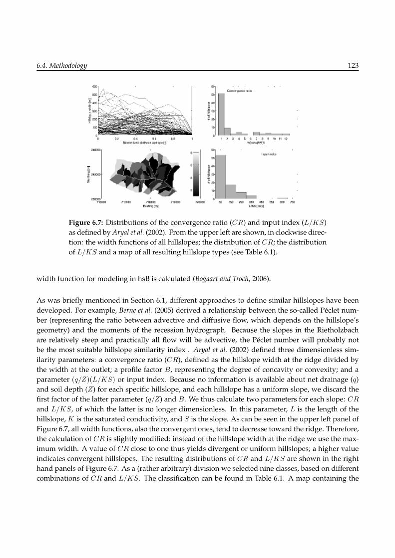
6.4. Methodology 123
Figure 6.7: Distributions of the convergence ratio (CR) and input index (L/KS)
as defined byAryal et al. (2002). From the upper left are shown, in clockwise direc-
tion: the width functions of all hillslopes; the distribution of CR; the distribution
of L/KS and a map of all resulting hillslope types (see Table 6.1).
width function for modeling in hsB is calculated (Bogaart and Troch, 2006).
As was briefly mentioned in Section 6.1, different approaches to define similar hillslopes have been
developed. For example, Berne et al. (2005) derived a relationship between the so-called Peclet num-
ber (representing the ratio between advective and diffusive flow, which depends on the hillslope’s
geometry) and the moments of the recession hydrograph. Because the slopes in the Rietholzbach
are relatively steep and practically all flow will be advective, the Peclet number will probably not
be the most suitable hillslope similarity index . Aryal et al. (2002) defined three dimensionless sim-
ilarity parameters: a convergence ratio (CR), defined as the hillslope width at the ridge divided by
the width at the outlet; a profile factor B, representing the degree of concavity or convexity; and a
parameter (q/Z)(L/KS) or input index. Because no information is available about net drainage (q)
and soil depth (Z) for each specific hillslope, and each hillslope has a uniform slope, we discard the
first factor of the latter parameter (q/Z) and B. We thus calculate two parameters for each slope: CR
and L/KS, of which the latter is no longer dimensionless. In this parameter, L is the length of the
hillslope,K is the saturated conductivity, and S is the slope. As can be seen in the upper left panel of
Figure 6.7, all width functions, also the convergent ones, tend to decrease toward the ridge. Therefore,
the calculation of CR is slightly modified: instead of the hillslope width at the ridge we use the max-
imum width. A value of CR close to one thus yields divergent or uniform hillslopes; a higher value
indicates convergent hillslopes. The resulting distributions of CR and L/KS are shown in the right
hand panels of Figure 6.7. As a (rather arbitrary) division we selected nine classes, based on different
combinations of CR and L/KS. The classification can be found in Table 6.1. A map containing the

124 6. A hillslope-based parameterization for sub-grid variability of topography
Table 6.1: Division of all 84 hillslopes in to 9 classes based on combinations of CR
and L/KS (Figure 6.7).
L/KS 100 L/KS
≤ < L/KS ≤ >
100 300 300
CR ≤ 2 1 2 3
2 < CR ≤ 7 4 5 6
CR > 7 7 8 9
resulting classes can be found in the lower left panel of Figure 6.7.
6.5 Results
Figure 6.8 showsmonthly values of actual evapotranspiration and discharge as simulated by all mod-
els in their aggregated version. In addition, the differences between the discharge simulations and
the observations are shown. hsB and TOPMODEL both use potential evaporation as calculated by
the Penman-Monteith equation (Penman, 1948; Monteith, 1965) as input. Due to an overestimation of
the amount of dew this potential evaporation is too low in winter. In addition, they are identical for
hsB and TOPMODEL because in winter no water limitation occurs. Because water limitation was as-
sumed not to occur in hsB, summer evapotranspiration is slightly overestimated. This overestimation
with respect to the lysimeter observations is relatively small (on average about 10 mm per month),
indicating that evaporation is mainly energy limited. The VICmodel also slightly overestimates sum-
mer evaporation, but winter evaporation is simulated accurately. The othermodels solving the energy
balance (hsB-LATS and TOPLATS) accurately simulate winter evaporation as well. Summer evapo-
ration as simulated by the latter models on the other hand is similar to that modeled by TOPMODEL
and significantly lower than observed, suggesting that the soil moisture reservoir in these models is
too small and water limited evaporation occurs too early.
Monthly values of discharge are reasonably close to the observed values, confirming that the model
calibration does not have a large influence on monthly values. This is further illustrated by Table 6.2,
where the performance of all models is summarized. Nash-Sutcliffe modeling efficiencies (E, Nash
and Sutcliffe, 1970) at monthly time steps are high (close to 0.8) for nearly all models except TOPLATS,
which appeared to have some initialization problems. In addition, Figure 6.9 shows the monthly
dynamics of other relevant variables, together with observations (when available). Observations are
available at one point (Buhl, Figure 6.1). Soil moisture observations were averaged over the three
available depths (Figure 6.2), and for groundwater only the dynamics should be compared because
the reference levels of the various water tables are different. For recharge and baseflow, all models
agree quite well, the dynamics are practically the same. For comparison with recharge, the lysimeter

6.5. Results 125
Table 6.2: Summary of model performances of all models employed in this study.
The Nash-Sutcliffe modeling efficiency (E), correlation coefficient (ρ), and the
relative volume error (RVE) are shown for hourly, daily and monthly timesteps.
The uncoupled hsB model and TOPMODEL were run with (C) and without (U)
correction for hillslope exposure.
Hourly Daily Monthly
E ρ E ρ E ρ RVE
[-] [-] [-] [-] [-] [-] [%]
VIC 0.61 0.80 0.74 0.87 0.83 0.93 -7.42
hsB
One slopeU 0.37 0.63 0.44 0.69 0.75 0.90 14.04
C 0.35 0.63 0.41 0.68 0.64 0.89 24.99
Two slopesU 0.48 0.70 0.56 0.76 0.76 0.90 13.54
C 0.46 0.70 0.54 0.76 0.66 0.90 24.40
All slopesU 0.53 0.74 0.64 0.81 0.76 0.90 14.64
C 0.51 0.73 0.61 0.80 0.66 0.90 25.20
ClassesU 0.48 0.70 0.57 0.77 0.76 0.90 14.19
C 0.49 0.71 0.58 0.77 0.76 0.90 13.79
TOPMODEL
One distr.U 0.72 0.87 0.80 0.91 0.81 0.92 8.71
C 0.72 0.88 0.79 0.92 0.77 0.91 14.49
Two distr.U 0.72 0.87 0.80 0.91 0.81 0.92 8.71
C 0.72 0.87 0.80 0.91 0.81 0.92 9.26
All pixelsU 0.72 0.87 0.80 0.92 0.81 0.92 8.71
C 0.72 0.88 0.79 0.92 0.77 0.91 14.49
TOP-LATSOne dist. C 0.21 0.63 0.46 0.73 0.32 0.68 -14.24
Two dist. C 0.25 0.63 0.48 0.73 0.34 0.69 -14.77
hsB-LATS
One slope C 0.30 0.55 0.37 0.61 0.76 0.87 -2.62
Open book C 0.34 0.59 0.42 0.65 0.77 0.88 -2.19
All slopes C 0.44 0.67 0.52 0.73 0.77 0.88 -5.18
Classes C 0.40 0.64 0.48 0.70 0.77 0.88 -6.01
drainage is plotted as well. Again the dynamics agree well, although simulated recharge is generally
somewhat lower than the lysimeter drainage.
The volumetric soil moisture content for TOPMODEL is estimated from the root zone storage deficit
assuming a porosity of 40%. Because the storage deficit is generally zero in winter, the moisture con-
tent is often equal to the porosity. This is in accordance with evaporation, which is at the potential rate
in winter (Figure 6.8). VIC and TOPMODEL show similar dynamics, although more pronounced for
TOPMODEL as explained above. The range in the observed soil moisture is much smaller, except for
a sudden (and rather suspicious) decrease in the summer of 2003 (Figure 6.2). TOPMODEL and VIC

126 6. A hillslope-based parameterization for sub-grid variability of topography
−50
0
50
100
150
ET
[mm
mon
th−
1 ]
a)
0
100
200
300
400
Dis
char
ge [m
m m
onth
−1 ]
b)
1999 2000 2001 2002 2003−150
−100
−50
0
50
100
150
∆ D
isch
arge
[mm
mon
th−
1 ] c)
Obs. VIC TOP hsB TOP−L hsB−L
Figure 6.8: Monthly evapotranspiration (a) and discharge (b) as simulated by five
models: hsB , hsB-LATS, TOPMODEL, TOPLATS and VIC. All models were used
in their aggregated version, i.e., one hillslope for hsB(LATS) and one distribution
of topographic indices for TOPMODEL/LATS. In c), differences between mod-
eled and observed discharge are shown. Observed evaporation is measured by
the lysimeter.
show this strong decrease as well, although slightly smoother. Soil moisture contents in TOPLATS
and hsB-LATS stay rather constant and do not show any decrease in 2003. Observations of water
table depth show an increasing trend until 2002, which is not captured by any of the models. Seasonal
and intra-seasonal dynamics are similar for all models. Not surprisingly, the simulated water tables
for hsB and hsB-LATS, and TOPMODEL and TOPLATS are very close together. Finally, for surface
runoff the dynamics are similar across the models, only TOPLATS exhibits much stronger peaks for
the extreme precipitation events.
Subsequently, the differences between the various levels of spatial aggregation for the different mod-
els are investigated, using the aggregated results that are shown in Figures 6.8 and 6.9 as the reference.
Figures 6.10, 6.11, 6.12, and 6.13 showdifferences between the aggregation levels for respectively TOP-
MODEL, hsB, hsB-LATS and TOPLATS. Figure 6.10 shows differences for simulations with and with-
out a correction for hillslope exposure, to isolate the effect of spatial aggregation. For TOPMODEL, it
was not feasible to correct the potential evaporation for every individual DEM-pixel. Therefore, the
simulations for every pixel and the distribution representing the entire catchment are both corrected

6.5. Results 127
0
50
100
150R
unof
f [m
m m
on−
1 ]a)
0
50
100
150
200
250 b)
Bas
eflo
w [m
m m
on−
1 ]
0.1
0.2
0.3
0.4 c)
Soi
l moi
stur
e [−
]
0
1
2
3d)
Wat
er ta
ble
dept
h [m
]
1999 2000 2001 2002 20030
100
200
300
Rec
harg
e [m
m m
on−
1 ]
e)
1999 2000 2001 2002 20030
100
200
300 f)P
rec.
[mm
mon
−1 ]
Obs. VIC TOP hsB TOP−L hsB−L
Figure 6.9: Monthly dynamics of other variables as simulated by five lumped
models and observations (when available): surface runoff (a), baseflow (b), soil
moisture (c), groundwater table (d), recharge (e) and precipitation (f). Note that
not all variables are simulated by all models, and no observations are available
for surface runoff and baseflow.
using the spatially averaged aspect. If no correction is applied, the changes in discharge appear to be
very small (typically less than 1%). This was to be expected, because all distributions of topographic
indices are very similar (Figure 6.3). When the correction for exposure is applied, overall evapotran-
spiration increases, causing an overall decrease of discharge. This, again, was to be expected given the
larger area of the southfacing distribution compared to the northfacing one (Figure 6.3). The decrease
in discharge can be attributed to similar decreases in both surface runoff and baseflow. Interestingly,
even when no correction for exposure is applied, the ratio between surface runoff and baseflow is
significantly different (up to 10%) between the simulation of one distribution and of all individual
pixels. This difference is, however, much smaller compared to the differences that are caused by hill-
slope exposure. This is caused by small-scale variability: the much larger variability of soil moisture
contents in the unsaturated zone reservoirs in the simulation for individual DEM-pixels (over 33000
DEM pixels compared to only 17 classes in the distribution; Figure 6.3) apparently causes more local
runoff, because this variability is “smoothed” in the lumped simulation. When aggregated tomonthly
values the increase in recharge and baseflow offsets this increase in runoff. It should be noted that rel-
ative differences are shown, so the large range in relative differences in surface runoff is compensated

128 6. A hillslope-based parameterization for sub-grid variability of topography
by the (apparently) much smaller range in relative differences of baseflow. Also at hourly timesteps,
however, the difference is too small to affect the hydrograph, because the statistics in Table 6.2 are
identical for all TOPMODEL simulations.
Figure 6.11 shows the differences in monthly discharge for simulations of two hillslopes (“open
book”), all 84 hillslopes, and the nine classes of similar hillslopes (Table 6.1) with respect to the aggre-
gated reference case. Again, results are compared with and without correcting for hillslope exposure.
In this case, each individual hillslope is corrected for its exposure, as opposed to the individual pixels
in TOPMODEL. Similar to TOPMODEL, the changes in catchment-average discharge are small (typ-
ically within ∼5%) compared to the single hillslope-case. Only in very dry conditions, when there
is barely any discharge, the relative difference increases. Examples are the late summer of 2003 and
the early summer of 2000 (Figure 6.8). The catchment-averaged discharge for hillslope classes is gen-
erally lower than that of the other simulations, due to higher evaporation (not shown). The reason
is that the majority of hillslopes that were taken as representative for their class were located at the
southfacing side of the catchment. When no correction is applied, the average of the classes is similar
to that of the open book and all hillslopes, illustrating the relatively large effect of hillslope exposure.
Where the differences between spatially averaged discharges at a monthly scale are negligible, they
are not at hourly and daily time steps, as can be seen in Table 6.2. Here, the resulting model efficien-
cies and correlation coefficients are significantly lower for the aggregated hillslope than for the other
simulations (E = 0.35 vs. E = 0.51 for individual slopes). According to these statistics, the “open
book”-simulation and the classes of similar hillslopes both proved to be better “aggregators”, with
E values of 0.46 and 0.49 respectively. This is the case with and without the correction for hillslope
exposure.
The coupled models (TOPLATS and hsB-LATS) were applied in a similar way as TOPMODEL and
hsB. Results for hsB-LATS can be found in Figure 6.12. As opposed to the uncoupled models, abso-
lute instead of relative differences are shown for better visibility. In addition to the weighted averages
of discharge and evapotranspiration, the variability across individual hillslopes and classes of simi-
lar hillslopes is shown. This variability is highly asymmetrical towards higher values for evaporation
and low values for discharge. This is caused by different land cover types, that were introduced in the
coupled models. Forested hillslopes evaporate significantly more than hillslopes with pasture land.
Because over the entire catchment the fraction of pasture land is much larger than that of forest (76%
vs. about 20%; see Figure 6.1b), this effect is relatively small but still significant in the catchment aver-
aged values. The inclusion of different land use types, therefore, causes structurally higher evapotran-
spiration and lower discharge in the simulations for individual hillslopes and classes compared to the
open-book and aggregated hillslopes. The reduction of 84 to 9 hillslopes by our (although quite rude)
classification yields practically the same results as the case where all individual hillslopes are com-
pared, both in terms of the catchment average and the variability across hillslopes. The same holds for
surface runoff, baseflow and the groundwater table, where the changes between the open book sim-
ulation and the aggregated case on one hand, and the individual hillslopes and classes on the other

6.5. Results 129
Figure 6.10: Differences in, from top to bottom, discharge, surface runoff, base-
flow, and evaporation as simulated by TOPMODEL. In the left panels, evapora-
tion is corrected for exposure, in the right panels this is not the case. The reference
situation is the “aggregated” version (one distribution of topographic indices;
Figure 6.8). Differences with respect to this reference are shown for the simu-
lation where all DEM-pixels have their own unsaturated zone reservoir (dash-
dotted lines), and the weighted average of the distributions containing north and
southfacing pixels (solid lines). The shaded area indicates the difference between
the simulated discharge for the distributions of northfacing and southfacing pix-
els. Negative values indicate lower values than the reference.
hand, show opposite signs. Surface runoff and baseflow for the open-book simulation only differ
during extreme precipitation events (see Figure 6.8), so relative differences are negligible. However,

130 6. A hillslope-based parameterization for sub-grid variability of topography
Figure 6.11: Differences in discharge as simulated by different versions of the
hsB model. The reference is the hsB simulation of one aggregated hillslope (Fig-
ure 6.8). Differences are shown for the weighted average of the “open-book” sim-
ulations (north- and southfacing hillslopes), the weighted average of all individ-
ual hillslopes, and that of classes of similar hillslopes. Negative values indicate
lower values than the reference. The light-shaded area represents the 10th and
90th percentiles of the individual hillslopes, the dark-shaded area indicates the
range between the north- and southfacing slopes and the thin grey lines indicate
the range of hillslope classes (see text for details).
simulation of individual hillslopes and classes yields more surface runoff, similar to TOPMODEL.
Changes in surface runoff are offset by those in baseflow at monthly scales, again as was the case
for the TOPMODEL simulations that were described before. These changes are practically identical
for the simulations of individual hillslopes and the classes of hillslopes. The Nash-Sutcliffe values
in Table 6.2 are, however, slightly higher for the open-book simulation (0.34 vs. 0.30 for the aggre-
gated hillslope). For the individual slopes and classes, the Nash-Sutcliffe values are, similar to hsB,
significantly higher: 0.44 and 0.40 respectively. Changes in moisture content and groundwater table
are structural, but very small. It is not clear why the changes in soil moisture have opposite signs for
individual hillslopes and hillslope classes. Similar results for TOPLATS can be found in Figure 6.13.
For the coupled version of TOPMODEL, simulations where the unsaturated zone model is resolved

6.5. Results 131
for each individual DEM pixel were not performed. Because the changes in discharge and evapotran-
spiration in the uncoupled TOPMODEL were very small, we expect that to be the case for the coupled
model as well. Indeed, in Figure 6.13 a similar structural increase in evaporation and decrease in dis-
charge can be seen as in Figure 6.10 when the open-book simulation is considered. For other variables,
differences are again very small.
Figure 6.12: Differences in six variables as simulated by different versions of hsB-
LATS. The reference is the simulation of one aggregated hillslope (Figure 6.8).
Differences are shown for the weighted average of the “open-book” simulations
(north- and southfacing hillslopes), the weighted average of all individual hill-
slopes, and that of classes of similar hillslopes. In a) and b), a light-gray shades
represent the 10th and 90th percentiles of all individual hillslopes, and dark-gray
shades represent the difference between the northfacing and southfacing slopes.
Thin grey lines, finally, indicate the range of hillslope classes (Table 6.1 and Fig-
ure 6.7). Negative values indicate lower values than the reference.

132 6. A hillslope-based parameterization for sub-grid variability of topography
Figure 6.13: Differences in six variables as simulated by different versions of
TOPLATS. The reference is the simulation of one distribution of values for the
topographic index representing the entire catchment. The black line indicates the
difference with the weighted average of the simulations for the distributions rep-
resenting the northfacing and southfacing pixels. The shaded area represents the
range between the latter two distributions. Negative values indicate lower values
than the reference.
6.6 Summary and conclusions
In the present study, a hillslope-based parameterization of small-scale heterogeneity is developed
and compared to other catchment parameterizations. The method is based on the hillslope-storage
Boussinesq model, that simulates saturated zone dynamics in a numerically efficient way, and takes
into account both advective and diffusive flow. The model is coupled to a similar formulation for the
unsaturated zone and energy balance as the TOPLATS land surface scheme to make it appropriate for
a land surface modeling context, and then applied to the small, alpine Rietholzbach catchment. To
investigate the influence of spatial aggregation on the model results, the method was applied at four
“aggregation levels”: (1) one large hillslope folded around the channel network; (2) two hillslopes

6.6. Summary and conclusions 133
(“an open book”); (3) nine classes of similar hillslopes, based on similarity parameters as defined by
Aryal et al. (2002), and (4) all individual hillslopes. This hillslope-based approach is compared with
the TOPMODEL approach, where pixels with similar hydrologic behavior are classified from a DEM
and the Variable Infiltration Capacity (VIC) approach, where a statistical relation between the fraction
of saturated area and the infiltration capacity is employed. TOPMODEL is also applied at three levels
of spatial aggregation: (1) one distribution of topographic indices; (2) two distributions, one repre-
senting all northfacing pixels and one representing all southfacing pixels, and (3) all individual DEM
pixels.
The hsB approach relaxes some assumptions that TOPMODEL requires. First, TOPMODEL assumes
that saturated zone dynamics can be described by successive steady-states. For small time steps this
is reasonable, but for larger time steps this may introduce errors. In this study, however, a fixed
time step of one hour was used for all models and the effect of this assumption was not investigated.
Second, TOPMODEL only takes into account advective or kinematic, and not diffusive flow. In this
study, however, this assumption is perfectly reasonable to make, because practically all hillslopes in
the Rietholzbach are very steep (20 to 30%). It would, therefore, be interesting to repeat this analysis
in another catchment with less steep, or even flat, slopes. In that case diffusive flow, which is taken
into account by hsB, would be much more important.
There are some issues that would require more research to make a hillslope-based parameterization
useful. Especially compared to numerically efficient approaches like VIC or TOPMODEL, the hsB-
LATS model is numerically quite demanding in the current formulation (programmed in Matlab).
Efficient programming in another computer language could significantly reduce run times. Further-
more, when the model is applied in areas such as the Rietholzbach with steep slopes, an analytical
solution for the kinematic wave approximation as developed by Troch et al. (2002) would yield practi-
cally identical results. In addition, the amount of hillslope classes could probably be further reduced
when carefully selecting similarity parameters. In less steep areas, for example, the Peclet number,
which represents the ratio of diffusive and advective flow (Berne et al., 2005; Lyon and Troch, 2007)
could be used. In this study, a rather arbitrary classification based on parameters proposed by Aryal
et al. (2002) was carried out. It would be worthwhile to further compare such similarity parameters in
different areas and under different conditions.
When catchment-averaged streamflow is considered, the effect of hillslope exposure is larger than
that of the level of spatial aggregation. When no correction for exposure is employed, the streamflow
is practically the same for all aggregation levels. When surface runoff and baseflow are considered
separately, however, it appears that there is more surface runoff when individual pixels are simulated
than when they are grouped in distributions. The same holds for individual hillslopes versus aggre-
gated hillslopes. At monthly time steps, this effect does not show up in the total discharge because it
is offset by the lower baseflow. At hourly and daily time steps, however, model efficiencies and cor-
relation coefficients suggest differences: the simulation of individual hillslopes achieves considerably
134 6. A hillslope-based parameterization for sub-grid variability of topography
higher efficiencies than the simulation with one large hillslope (0.52 vs. 0.36 respectively, at hourly
time steps). Inclusion of the unsaturated zone and energy balance enables more accurate simulation
of monthly evaporation, but this does not show up in the resulting discharge: modeling efficiencies
are quite low. Also in hsB-LATS, however, efficiencies are highest when all individual slopes are mod-
eled. Obviously, the models should be recalibrated to some extent after introducing the unsaturated
zone and energy balance formulations. Now, the model parameters obtained from calibrating the
uncoupled models (Figure 6.5) were employed.
Based on these results, it cannot be concluded that one of the investigated approaches is better than
the others. The VIC model, with its statistical representation of small-scale variability, captured
catchment-averaged processes reasonably well; monthly evaporation was modeled accurately and
also discharge was simulated well. Discharge simulations by hsB are comparable to others at monthly
scales, but at hourly time steps model efficiencies are relatively low, which is not surprising given the
fact that no unsaturated zone was taken into account. At hourly time steps TOPMODEL reached the
highest model efficiencies; its low complexity makes it easy to parameterize and in this terrain its
basic assumptions are valid. For both hsB and hsB-LATS modeling efficiencies were highest when
the maximum amount of spatial detail was incorporated (i.e., hillslopes were modeled individually).
For both models, reducing the number of hillslopes by grouping similar hillslopes together (from 84
to 9) yields very similar catchment-averaged fluxes and also the variability across hillslopes is similar
compared to the simulation of all individual hillslopes. This is much less the case for aggregation of
the catchment into one or two hillslopes. Given the steep slopes of this terrain, the advantage of hsB
with respect to TOPMODEL (inclusion of diffusive flow) does not really play a role, and the effect of
groundwater on soil moisture variability through capillary uprise will probably also be small, hence
the small differences between the models. As mentioned before, it would be interesting to repeat the
analysis for a different catchment with less steep slopes.
Acknowledgements
This research was supported by the European Commission through the FP6 Integrated Project NeWa-
ter (http://www.newater.info) and the BSIK ACER project under the Dutch Climate Changes Spatial
Planning programme.

Chapter 7
General discussion

7.1. Introduction 137
7.1 Introduction
In this thesis, a land surface model, the Variable Infiltration Capacity (VIC; Liang et al., 1994) model,
was employed to investigate and quantify the effects of land use change (Chapter 3), climate change
(Chapter 4) and oscillations in ocean temperature (Chapter 5) on the hydrological system. To jus-
tify using the VIC model, its performance was assessed by comparing model results with those of a
conceptual water balance model (STREAM; Aerts et al., 1999), and observations in the Rhine basin
(Chapter 2). An important feature of the VIC model, its parameterization of small-scale heterogeneity
of soil moisture within a model grid cell, was compared with alternative parameterizations in Chap-
ter 6. In the remainder of this chapter, the advantages and disadvantages of the VIC model compared
to other models are discussed in Section 7.2, whereas the uncertainties involved in the model input
are discussed in Section 7.3. Themain conclusions from the thesis are drawn in Section 7.4 and, finally,
in Section 7.5, some directions for further research are suggested.
7.2 Discussion of the hydrological model
In the VIC model, the representation of land-atmosphere interactions (evapotranspiration) is rela-
tively physically-based, whereas that of subsurface hydrological processes is more conceptual and
simplistic (Liang et al., 1994). At the scale of large river basins such as the Rhine or the Colorado,
however, it is not feasible to take into account these hydrological processes in detail, because there is
simply too much heterogeneity. At this large scale, conceptual hydrological models often perform as
good as or better than complex physically-based hydrological models (e.g., Sivalapan, 2003; te Linde
et al., 2008), because the theory that physically-based models are based on is usually only valid at
small scales (McDonnell et al., 2007). Models that have often been used to model the water budget
in large river basins, such as HBV or STREAM (see Chapter 2 for details), simplify both subsurface
hydrological processes and land-atmosphere interactions, making them relatively fast and easy to
operate. The physically-based approach to calculate evapotranspiration in VIC, however, provides a
potential for more accurate evapotranspiration and thus also streamflow simulations, since the two
are closely linked through the water balance (e.g., Koster et al., 2000).
In Chapter 2, this potential is investigated by comparing streamflow simulations of the VIC and
STREAMmodels in the Rhine basin. In addition, a model of intermediate complexity is introduced by
applying the VIC model in the water balance mode (i.e., the energy balance is not resolved), denoted
as VIC-WB. As atmospheric forcing for all models, downscaled re-analysis data (i.e., atmospheric
model output combined with observations) was used. This dataset was shown to have a bias com-
pared to observations, causing relatively poor modeling efficiencies for all models. Results showed
that the STREAM model is more sensitive to calibrated parameter values, and thus more effectively
compensated for erroneous forcing data in the calibration period, causing poor performance in the
validation period. For the validation period, the sub-grid variability that is accounted for in VIC-WB,

138 7. General discussion
as opposed to STREAM, results in improved streamflow simulation compared to STREAM. Similar
to STREAM, however, VIC-WB is relatively sensitive to model calibration parameters.
Including the energy balance and reducing themodel time step from 1 day to 3 hours (i.e., running the
full VIC model) further improves extreme streamflow simulation, and significantly improves simula-
tion of evapotranspiration. Furthermore, the model’s robustness is increased, which is important for
impact assessments of climate change and land use change, since it is highly questionable whether pa-
rameter values that were obtained from calibration under current conditions are valid under changing
conditions. VIC’s physically-based parameterization for evapotranspiration and vegetation provides
an additional advantage: parameter values are physically-based as well and can be related to physical
vegetation properties. This is much less the case for models such as STREAM, where evapotranspira-
tion is estimated from temperature only.
7.3 Discussion of the climate and land use change scenarios
All land use change scenarios and climate scenarios that have been used in this thesis are based on
storylines of socio-economic and technological developments and the associated CO2-emissions that
were composed by the Intergovernmental Panel on Climate Change (IPCC; IPCC, 2000). Four land
use change scenarios were obtained from the Eururalis project (Verburg et al., 2006b). They were cre-
ated using a set of models that take into account economic and demographic developments, and
allocate land use types to individual pixels of 1 km2, resulting in land use maps for the year 2030.
The effect of changing climate conditions is only taken into account through an increase in tempera-
ture, not precipitation. Many previous land use change impact assessments used historical data (e.g.,
Matheussen et al., 2000), or hypothetical scenarios, for example a doubling of urban area (Hundecha and
Bardossy, 2004). The scenarios that were used in Chapter 3 are, therefore, among the most “realistic”
scenarios available.
In Chapter 4, three climate scenarios were used that are based on the same IPCC storylines as the
land use change scenarios. To obtain the actual changes in climate that are associated with each CO2-
emission scenario, Global Climate Models (GCMs) are used. Because their spatial resolution is too
low for hydrological applications, Regional Climate Models (RCMs) are necessary to downscale the
GCM-output to a higher resolution. Several GCMs and RCMs have been developed, and they gener-
ally give very different results, even in reproducing the current climate (e.g., Covey et al., 2003; Reichler
and Kim, 2008). Understandably, the range in projected scenarios is even larger. In addition, precipi-
tation, which is the most critical variable for hydrological applications, is a very difficult variable to
simulate in climate models. Most climate models, for example, tend to overestimate the amount of
“drizzle” (Perkins et al., 2007; Sun et al., 2006). As a result, climate model output typically has a bias
compared to observations that should be corrected for (Lenderink et al., 2007).

7.4. General conclusions 139
Several ways exist to do this (e.g., Leander and Buishand, 2007; Hay et al., 2002). In Chapter 4, a rela-
tively simple, non-linear correction is applied that corrects the bias, taking into account its spatial and
temporal variations (Leander and Buishand, 2007). Not only the climate scenarios that were used in this
thesis were found to be biased with respect to the observations, but also the re-analysis data that were
used in Chapters 2 through 4. Their bias is, however, different than that of the scenarios, because the
driving model behind it is different. It should be noted that the precipitation and temperature fields
are strongly influenced by the bias correction in the sense that the spatial patterns of the model output
are “drawn” towards those of the observations. Furthermore, because no information is available for
the future, the model bias is generally assumed to be constant in time. Recent research by Christensen
et al. (2008) indicated, however, that the bias tends to grow with increasing temperatures, resulting in
an overestimation of the climate change signal. This should be kept in mind while interpreting the
results of Chapter 4.
Ideally, ensembles of models, both of GCMs and RCMs, should be used, because the multi-model
mean is generally a better predictor than individual models (Lambert and Boer, 2001). In this the-
sis, however, scenarios by only one GCM and one RCM were available at a high spatial resolution.
Moreover, use of multiple models would not been feasible numerically. The GCM that was used in
Chapter 4, ECHAM5-OM, does very well in reproducing the current climate (Reichler and Kim, 2008).
It is, however, more sensitive to aerosol concentrations than most other GCMs, causing it to be rela-
tively cool in the first half of the 21st century due to the “dimming” effect of the aerosols. After 2050,
aerosol concentrations decline, causing a stronger temperature increase in ECHAM5-OM compared
to other GCMs (IPCC, 2007). This feature partly explains the contrast between the first and second
halves of the 21st century that was found in Chapter 4.
7.4 General conclusions
In Chapter 2, the VIC model was found to simulate extreme streamflow reasonably well, and to be
less sensitive to calibrated parameter values than the STREAM model. In addition, the fact that its
evapotranspiration parameters directly represent vegetation properties also makes it easier to inves-
tigate the impact of land use changes. Therefore, the VIC model was used for impact assessments of
land use change and climate change, which are described in Chapter 3 and 4, respectively. To isolate
the effects of both changes, in Chapter 3 the atmospheric forcing was kept constant, whereas in Chap-
ter 4 the land use was kept constant. The atmospheric forcing in Chapter 3 was identical to that in
Chapter 2, namely a downscaled re-analysis dataset.
140 7. General discussion
7.4.1 Effects of land use change
Based on simulations of a single grid cell covered by different land use types, as described in Chap-
ter 3, the VICmodel’s original formulation for evapotranspiration was slightly altered. In the original
model, no bare soil evaporation is allowed when a land use tile is classified as vegetated. However,
for sparsely vegetated areas, such as cropland in winter season, this causes underestimations of evap-
otranspiration. By introducing a fractional bare soil evaporation, which exponentially depends on the
leaf area index, the representation of annual total evapotranspiration as well as its annual cycle is im-
proved. In addition, a crude parameterization for water management in urban areas was introduced
by changing the value of the hydraulic conductivity and thus tuning the amounts of surface runoff
and baseflow in urban areas. The modified model was then used to investigate the effects on average
and extreme streamflow of six land use change scenarios at various locations in the Rhine basin. Two
scenarios were hypothetical and not very realistic: all agricultural land was turned into either forest
or grass. The remaining four scenarios are realistic future scenarios (Section 7.3).
Results showed that the future land use scenarios (Eururalis) generally indicated an increase in stream-
flow, mainly due to urbanization. Effects of urbanization are quite small, however, because they are
partly compensated by a decrease of cropland and small increases in grassland, forest and natural
area (e.g., shrubs). Conversion of agricultural land to forest or grass yielded a decrease in streamflow
in both cases because of increased evapotranspiration. When considering streamflow at the basin
outlet, the effects are small, but the effects on streamflow from small tributaries can be significant.
These results are consistent with previous studies; for example Hundecha and Bardossy (2004) found
considerable effects of land use changes on streamflow from small sub-basins in the Rhine. Bronstert
et al. (2002), on the other hand, found that the effect of land use change on streamflow in the main
branch of the Rhine is very small.
7.4.2 Effects of climate change
The effects of climate change on streamflow in the Rhine basin are much larger than those of land use
changes, as demonstrated in Chapter 4. In previous studies, Kwadijk and Rotmans (1995) and Shabalova
et al. (2003) found increases in winter streamflow of about 30%, and decreases in summer streamflow
of 30 to 40% by the end of the 21st century. The study presented in Chapter 4 differs from previous
studies in that the spatial resolution of the employed atmospheric data is higher, and that a time pe-
riod spanning the entire 21st centurywas analyzed instead of a relatively small time slice. Simulations
by the VIC model of three climate scenarios for the periods 2001–2050 and 2051–2100 were compared
with a simulation of the reference period, 1951–2000. Each climate scenario was based on a differ-
ent CO2-emission scenario: A2, A1B and B1 (Section 1.1.3). All atmospheric data were dynamically
downscaled by an RCM to a spatial resolution of 0.088 degrees, or ∼10 km, and corrected for the
bias with respect to the observations as discussed in Section 7.3. The downscaled and bias-corrected
re-analysis dataset that was also used in Chapters 2 and 3 was then used to calibrate the hydrological

7.4. General conclusions 141
model. Results indicate average streamflow at the basin outlet to increase by 30% in winter and spring
and to decrease with a similar value in summer and autumn at the end of the century. These results
thus confirm previous studies (e.g., Kwadijk and Rotmans, 1995; Shabalova et al., 2003). The majority of
this change originates in the Alpine part of the catchment, and is caused for a large part by a decrease
of the contribution of snowmelt to streamflow and by a shift of the timing of the snowmelt season to
earlier in the year. Furthermore, the high-resolution climate scenarios and the distributed hydrologi-
cal model allow for a detailed analysis of spatial patterns. Results indicate that the projected decrease
in summer discharge is concentrated in the southern part of the basin. The northern tributaries, where
there is hardly any decrease in summer precipitation, are dominated by wetter conditions throughout
the year. In addition, our results reveal an interesting contrast between the first and second half of
the 21st century. In all three scenarios, the first half is dominated by relatively wet conditions and
more extreme peak flows. During the second half of the century, temperature and evapotranspira-
tion increase drastically, causing generally dryer conditions and more extreme streamflow droughts.
To some extent, this contrast can be explained by the GCM that was employed, as discussed in Sec-
tion 7.3.
7.4.3 Effects of oscillations in ocean temperature
In addition to the aspect of climate change discussed in Section 7.4.2, there is also climate variability
originating from interannual to (inter)decadal cycles in Pacific and Atlantic ocean temperatures. In
some areas of the world, these cycles affect the climate system and water resources through telecon-
nections (e.g. Mason and Goddard, 2001; Power et al., 2006). In the Colorado River Basin (CRB), pre-
cipitation and streamflow have been linked to ENSO (El Nino-Southern Oscillation) and PDO (Pacific
Decadal Oscillation), for example by Redmond and Koch (1991) and Canon et al. (2007). In Chapter 5, the
CRB is used as study area to assess the influence of Pacific ocean temperature variability on several
hydrologic variables, such as precipitation, snow cover, soil moisture and groundwater. Data was
extracted from a simulation by the VIC model spanning 74 years (1930–2003) and related to climate
indices describing the variability of ocean temperatures in the tropical and extra-tropical Pacific ocean.
Results show that precipitation, soil moisture and discharge are all related to ENSO in the southern
part of the basin, mainly in winter and spring. ENSO in summer is correlated to summer precipita-
tion, moisture and discharge throughout the CRB, as was also found by Hidalgo and Dracup (2003).
The relation between these variables and ENSO and PDO are strongest during phases of extremely
warm (cool) ocean temperatures, known as El Nino (La Nina).
The PDO has different cycles of variability. One with a relatively high frequency that is correlated
with ENSO, and another spanning very long periods, even multiple decades, which are generally
known as PDO phases. During the 74 years of study, two transitions to a different PDO phase have
taken place, one in 1946 and one in 1976. Results show that a strong connection exists between hydro-
logical conditions in the CRB and this low-frequency model of PDO. Smoothed storage anomalies of

142 7. General discussion
groundwater and the surface reservoir of LakeMead appeared to be strongly correlated with PDO, as
were the amplitudes of the anomalies of soil moisture and runoff, indicating drier conditions during
negative PDO phases. Although the mechanisms and exact periodicity behind PDO is not yet well
understood (Newman, 2007), and its predictability is low, data indicates that a new regime shift to a
negative phase may have occurred in the late nineties (Mantua and Hare, 2002). If that is the case, then
the current dry conditions in the CRB may dominate for several more years or even decades.
7.4.4 An alternative parameterization for small-scale variability of soil moisture
The representation of (subsurface) hydrological processes in the VIC model is conceptual and, com-
pared to the formulation for land-atmosphere interactions, relatively simplistic. As an alternative
parameterization for small-scale variability of topography, a catchment, or large-scale grid cell, can
be divided into hillslopes. Each class of hydrologically similar hillslopes can then be modeled using
the hillslope-storage Boussinesq (hsB) model. The dynamics of the water table and its influence on
soil moisture variability is then taken into account as well. This approach, along with the VIC model,
was applied to a small, alpine catchment, the Rietholzbach. In addition, TOPMODEL was applied,
which makes use of hydrologic similarity as well, but based on individual pixels from digital terrain
information. The models were applied at different levels of spatial aggregation: individual hillslopes,
classes of similar hillslopes, two opposite hillslopes and the catchment represented as one hillslope.
The larger variability of soil moisture contents that results from simulations of individual hillslopes
yields more generation of surface runoff in all models. On monthly scales, however, this increase is
compensated by decreasing baseflow. Therefore, changes in discharge are small. On daily and hourly
time steps, this compensation does not take place. Therefore, the simulations with individual hill-
slopes achieve the highest modeling efficiencies when catchment-averaged streamflow is compared
to observations. When the number of hillslopes is reduced from 84 to 9 classes of similar hillslopes,
the simulation of catchment-averaged discharge, as well as the variability across hillslopes is similar
to the case when all hillslopes are simulated explicitly. Division of hillslopes into such classes is a bet-
ter way of aggregating then representing the catchment as one big hillslope. The statistical approach
of VIC accurately simulated both discharge and evaporation. It is able to represent the processes
associated with soil moisture variability in the Rietholzbach to a sufficient extent, although it is not
physically-based and groundwater is not included.
7.5 Directions for further research
In this thesis, effects of land use change and climate change were assessed separately, i.e., climate
conditions were kept constant for all land use scenarios and vice versa. It might well be that under
extreme climate conditions such as predicted by climate scenarios, the land use affects streamflow in

7.5. Directions for further research 143
a different way. Therefore, a logical next step would be to perform a combined analysis. For example,
for each SRES storyline the associated climate scenarios and land use scenarios could be simulated
simultaneously. Or, to limit computation time, extremely wet or dry episodes from the climate sce-
narios could be selected to evaluate the effects of land use changes under extreme conditions. Even
better would be to represent vegetation dynamically and fully interactive, as is done for example at
the global scale in the LPJ (Lund-Potsdam-Jena) model (Gerten et al., 2004; Bondeau et al., 2007).
The climate scenarios that were used in Chapter 4 were obtained from only one GCM, whereas ide-
ally an ensemble of models should be used, as was already discussed in Section 7.3. According to
GCM intercomparison experiments, multi-model means better represent current climate conditions
and provide more realistic climate scenarios, because the specificities of individual models are aver-
aged out (e.g. Covey et al., 2003; Reichler and Kim, 2008). Furthermore, in this thesis the hydrological
model is run “offline”. This causes inconsistencies, i.e., the evaporative fluxes from the land to the at-
mosphere as simulated by the VICmodelmay be (and probably are) different than those simulated by
the original land component of the climate model. Ideally, one should carry out a similar experiment
where the climate model and the hydrological model are coupled, to prevent inconsistencies and cap-
ture important feedbacks from soil moisture on precipitation and temperature (e.g. Seneviratne et al.,
2006).
Throughout this thesis, extreme peak flows and low flows have been analyzed. The length of the
simulated time series used to obtain estimates of the extremes was relatively short (3 times 100 years
at most). Flood peaks that are relevant for water management, for example the design discharge,
have a return period of 1250 years for the Rhine basin (Eberle et al., 2002). To make a statistically
reasonable estimate of the design discharge, much longer time series spanning about 10.000 years
would be necessary. It is obvious that such time series cannot be obtained from observations, and
not (yet) from climate model simulations. A rainfall generator (Beersma, 2002; de Wit and Buishand,
2007), can create such time series by statistical resampling. In many applications, however, observed
data are resampled. Maximum daily rainfall amounts are, therefore, not allowed to exceed those in
the observed record, which is not very realistic under changing climate conditions. At the moment,
applying such a rainfall generator to (bias corrected) climate model output seems to be the best option.
A relevant improvement of the hydrological model to simulate extreme streamflow droughts would
be to improve the representation of groundwater. In many large-scale hydrological models, such as
the VIC model, groundwater flows are not explicitly modeled and also the influence of groundwater
on soil moisture through capillary uprise is not taken into account. Recently, these processes have
been implemented in land-surface models (e.g.Maxwell and Kollet, 2008; Fan et al., 2007;Miguez-Macho
et al., 2007), but at the scale of large river basins such as the Rhine or Colorado this is not feasible (yet).
In some parts of the world, large-scale climate oscillations have a significant influence on the hydro-
logical system through teleconnections. However, the current level of understanding of the physics

144 7. General discussion
behind these is limited, and often the frequency of oscillation is low (for example PDO), so only few
“transitions” have occurred in the observed record. Accurately predicting these oscillations and the
relations between them is still extremely difficult (Newman, 2007). To improve our understanding and
their predictability more research is needed, because they are crucial for water management in, for
example, the Colorado River Basin. To encrease the length of the available time series, paleohydro-
logical and -climatological records can be used for this research, as was already done by, for example,
MacDonald and Case (2005) and Rasmussen et al. (2006).
Because the effect of land use changes in the Rhine basin was shown to be quite small, it does not
seem to be a relevant option for water managers to mitigate extreme floods or low flows. However,
because effects in sub-basins can be significant, an effective combination of different land use changes
in different parts of the basin could be able to alter the magnitude of low-flows and/or timing of flood
peaks at the basin outlet. Other management options to locally mitigate hydrological extremes could
take place in urban areas: so-called “green roofs” and ponds can help to increase storage capacity in
upstream areas. In Chapter 3 a crude parameterization to evaluate the effects of such measures was
implemented. A more refined parameterization was suggested by Cuo et al. (2008), and it is part of
ongoing research to implement such a parameterization in the VIC model and further investigate to
what spatial extent these measures can influence streamflow.
For most of the additional simulation experiments that are suggested above, an important limiting
factor is computation power. Simulating time series spanning hundreds of years at a high spatial and
temporal resolution is very time consuming. The amount of time needed increases fast when multi-
ple simulations are needed for model calibration or to get an idea of the uncertainty that is involved.
As computing power keeps increasing and more and more multi-processor clusters get more readily
available, the suggested simulations become easier to carry out.
Concerning the parameterization of small-scale variability that was discussed in Chapter 6, there
are also some issues that would be interesting to investigate more in-depth. The hillslope-based ap-
proach, as opposed to the TOPMODEL-approach, takes into account both diffusive and advective
flow. In the Rietholzbach, where slopes are generally steep, diffusive flow does not effectively play
a role and this advantage is not of interest. Therefore, it would be interesting to repeat the analysis
of Chapter 6 for a catchment with less steep slopes, or even no slopes at all. Moreover, the choice
of similarity parameters to classify the hillslopes could be investigated further. Although our rather
arbitrary method based on Aryal et al. (2002) yielded promising results, it would be interesting to see
whether results change when all the parameters defined by Aryal et al. (2002) are taken into account
instead of just two. In areas with less steep slopes, also the Peclet number, representing the ratio
between advective and diffusive flow (Berne et al., 2005) could be used. These are just examples; a
significant amount of research has recently been and will be devoted to this subject (e.g. Sivalapan,
2003; Wagener et al., 2007; Tetzlaff et al., 2008).

Chapter 8
Nederlandse samenvatting


8.1. Inleiding 147
8.1 Inleiding
De globaal gemiddelde temperatuur is de afgelopen tientallen jaren dusdanig gestegen, dat dit naar
verwachting een grote invloed heeft op het klimaatsysteem en de hydrologische cyclus (IPCC, 2007).
Omdat warme lucht een grotere verzadigde dampdruk heeft en meer waterdamp kan bevatten dan
koude lucht wordt verwacht dat verdamping en neerslag verwacht toenemen. Ook kan de frequentie
en omvang van extreme neeslaggebeurtenissen groter worden (Trenberth, 1997a). Bovendien kun-
nen de hydrologische effecten van deze veranderingen versterkt of verzwakt worden door landge-
bruiksveranderingen zoals bebossing en urbanisatie (bv. Bradshaw et al., 2007). In dit proefschrift
wordt een land-oppervlaktemodel, het Variable Infiltration Capacity model (VIC; Liang et al., 1994),
toegepast om de effecten van landgebruiksverandering (Hoofdstuk 3), klimaatverandering (Hoofd-
stuk 4) en oscillaties in oceaantemperatuur (Hoofdstuk 5) te onderzoeken en te kwantificeren. Om
het gebruik van het VIC model te rechtvaardigen, zijn de prestaties ervan onderzocht door modelre-
sultaten van het VIC model te vergelijken met die van een conceptueel waterbalansmodel (STREAM;
Aerts et al., 1999) en observaties in het Rijnstroomgebied (Hoofdstuk 2). Een belangrijk aspect van het
VIC model, namelijk de parametrisatie van kleinschalige bodemvochtvariabiliteit binnen een model-
gridcel, is vergelekenmet soortgelijke parametrisaties in Hoofdstuk 6. Het vervolg van dit hoofdstuk
is als volgt opgebouwd: in Sectie 8.2 worden de voor- en nadelen van het VICmodel ten opzichte van
andere modellen bediscussieerd; in Sectie 8.3 worden de onzekerheden omtrent de invoerdata voor
hetmodel beschreven, en in Sectie 8.4 tenslotteworden de belangrijkste conclusies van dit proefschrift
samengevat en in perspectief geplaatst.
8.2 Het hydrologisch model in perspectief
In het VICmodel is de berekening van de uitwisseling van vocht en warmte tussen land en atmosfeer,
onder meer de verdamping, relatief complex en fysisch gebaseerd vergeleken met die van (onder-
grondse) hydrologische stromingsprocessen, die relatief conceptueel en simplistisch is (Liang et al.,
1994). Op de schaal van grote rivierstroomgebieden zoals de Rijn of de Colorado, is het echter erg
moeilijk om deze processen in detail en expliciet te modelleren omdat er simpelweg teveel hetero-
geniteit is in de eigenschappen van bodem, vegetatie en topografie die deze processen aansturen. Op
deze schaal presteren conceptuele, simplistische modellen vaak even goed of zelfs beter dan com-
plexe, fysisch gebaseerde modellen die wel proberen hydrologische processen in detail te simuleren
(Sivalapan, 2003; te Linde et al., 2008). Een van de redenen hiervoor is het feit dat de theorie die meestal
ten grondslag ligt aan fysisch gebaseerde modellen alleen geldig is op kleine schaal of zelfs een punt
(McDonnell et al., 2007).
In studies die de invloed van klimaatverandering op de hydrologie onderzoeken, worden vaak mod-
ellen gebruikt die zowel de zojuist genoemde hydrologische stromingsprocessen als de uitwisseling
met de atmosfeer via verdamping vereenvoudigen. Voorbeelden zijn HBV en STREAM (zie Hoofd-

148 8. Nederlandse samenvatting
stuk 2 voor meer details). Deze modellen zijn daarom vaak eenvoudig en snel toe te passen. De
meer fysische gebaseerde berekening van verdamping in VIC kan mogelijk echter nauwkeurigere
schattingen van de verdamping geven. Omdat afvoer en verdamping sterk gekoppeld zijn via de wa-
terbalans, kan afvoer dus ook nauwkeuriger berekend worden (bv. Koster et al., 2000). In Hoofdstuk 2
wordt dit nader onderzocht door afvoersimulaties van de VIC en STREAM modellen te vergelijken.
Daarnaast wordt eenmodel geıntroduceerdmet een tussenliggende complexiteit door het VIC model
toe te passen in de zogenaamde waterbalans-variant (VIC-WB), wat betekent dat de energiebalans
niet wordt opgelost.
Als atmosferische invoerdata voor alle drie de modellen is her-analysedata gebruikt (dit is uitvoer
van een atmosferisch model waarin waarnemingen zijn verwerkt), die vervolgens met een region-
aal klimaatmodel zijn neergeschaald naar een hoge ruimtelijke resolutie (ongeveer 10 km). Deze
her-analysedataset wijkt echter sterk af van geobserveerde neerslag en temperatuur, zo wezen de
resultaten van een vergelijking uit, waardoor de kwaliteit van de gesimuleerde afvoer ten opzichte
van de waargenomen afvoer voor alle drie de modellen relatief laag was. Het STREAMmodel bleek
verder gevoeliger te zijn voor de gecalibreerde parameterwaarden dan het VIC model. Het com-
penseerde dus ook effectiever voor de afwijkingen in de neerslaginvoer ten opzichte van waarne-
mingen die aanwezig waren in delen van de calibratieperiode, hetgeen weer lagere modelleringsef-
ficienties gedurende de validatieperiode veroorzaakte.
De parametrisatie van sub-pixel variabiliteit die wordt meegenomen in het VIC-WB model, in tegen-
stelling tot het STREAMmodel, resulteert in verbeterde afvoersimulaties vergelekenmet het STREAM
model voor de validatieperiode. Het VIC-WB model is echter, net als het STREAMmodel, gevoeliger
voor gecalibreerde parameterwaarden. Het meenemen van de energiebalans en het verkleinen van
de tijdstap van 1 dag naar 3 uur (zoals in het VIC model gebeurt) verbetert de afvoersimulaties
nog verder, en levert ook een significante verbetering van de simulatie van verdamping op. Het
VIC model blijkt robuuster te zijn vergeleken met de andere modellen (minder gevoelig voor cali-
bratieparameters), hetgeen belangrijk is voor onderzoeken naar de effecten van klimaat- en landge-
bruiksveranderingen. Het is namelijk sterk de vraag of parameterwaarden die bepaald zijn door
calibratie onder de huidige condities nog geldig blijven onder veranderende omstandigheden. De
fysisch gebaseeerde berekening van verdamping en vegetatie biedt bovendien een ander voordeel:
de parameterwaarden hebben een fysische basis en kunnen gerelateerd worden aan fysische eigen-
schappen van de vegetatie. Dit is in veel mindere mate het geval voor STREAM, waar verdamping
alleen uit temperatuurgegevens wordt geschat.
8.3 De landgebruiks- en klimaatveranderingsscenarios in perspectief
Alle landgebruiksveranderings- en klimaatscenarios die in dit proefschrift zijn gebruikt zijn gebas-
eerd op verhaallijnen die verschillende sociaal-economische en technologische ontwikkelingen en de

8.3. De landgebruiks- en klimaatveranderingsscenarios in perspectief 149
daarmee gepaard gaande CO2-emissies beschrijven. Deze verhaallijnen zijn samengesteld door het
Intergovernmental Panel on Climate Change (IPCC; IPCC, 2000). De vier gebruikte verhaallijnen
worden weergegeven als A2 (“Continentale markten”), A1 (”Globale economie”, waar bij het hier ge-
bruikte subscenario A1B aangeeft dat er balans is tussen fossiele en duurzame energie), B1 (“Globale
samenwerking”) en B2 (“Regionale gemeenschappen”). Vier landgebruiksveranderingsscenarios, elk
gebaseerd op een van deze vier verhaallijnen, zijn gebruikt zoals ze zijn samengesteld in het kader van
het Eururalis project (Verburg et al., 2006b). Deze werden gecreeerdmet eenmodellenset die economis-
che en demografische ontwikkelingen gebruikt om ontwikkelingen in landgebruik te voorspellen, en
de resulterende landgebruikstypen aan individuele pixels van 1 km2 toewijst. Dit resulteerde in vier
landgebruikskaarten voor het jaar 2030. Het effect van klimaatverandering op landgebruik is alleen
meegenomen door een stijging van temperatuur, niet van neerslag. Eerdere effectstudies van landge-
bruiksveranderingen gebruikten historische data (bv.Matheussen et al., 2000) of hypothetische scenar-
ios zoals een verdubbeling van het stedelijk gebied (Hundecha and Bardossy, 2004). De scenarios die
zijn gebruikt in Hoofdstuk 3 behoren bij de meest realistische scenarios die beschikbaar zijn.
InHoofdstuk 4 zijn drie klimaatscenarios gebruikt die elk zijn gebaseerd op een andere IPCC-verhaallijn,
in volgorde van oplopende CO2 emissies: B1, A1B en A2. Om de feitelijke verandering in klimaat te
verkrijgen die gekoppeld is aan elk CO2 emissiescenario worden globale klimaatmodellen (GCMs)
gebruikt. Omdat de ruimtelijke resolutie daarvan veel te laag is voor hydrologische toepassingen
zijn regionale klimaatmodellen (RCMs) nodig om de uitvoer van GCMs om te zetten naar een hogere
resolutie. Er zijn verschillende GCMs en RCMs ontwikkeld en zij geven meestal erg verschillende
resultaten, zelfs als zij het huidige klimaat proberen te reproduceren (bv. Covey et al., 2003; Reichler
and Kim, 2008). De bandbreedte van geprojecteerde klimaatscenarios is, zoals te begrijpen is, nog
groter. Bovendien is neerslag, de meest kritieke variabele voor hydrologische toepassingen, voor kli-
maatmodellen erg moeilijk te simuleren. De meeste modellen hebben bijvoorbeeld de neiging om de
hoeveelheid motregen te overschatten (Perkins et al., 2007; Sun et al., 2006). Klimaatmodellen hebben
daarom bijna altijd een structerele fout ten opzichte van waarnemingen die gecorrigeerd moet wor-
den (Lenderink et al., 2007). Er bestaan verschillendemanieren omdit te doen (bv. Leander and Buishand,
2007; Hay et al., 2002).
In Hoofdstuk 4 is een relatief eenvoudige, niet-lineaire correctie toegepast die de structurele fout op
een ruimtelijk en temporeel variabele manier corrigeert. Niet alleen de klimaatscenarios vertonen
een structurele fout, maar ook de her-analyse data die zijn gebruikt in Hoofdstukken 2 tot en met
4. Deze fout is echter anders dan die van de scenarios omdat het model waar de her-analyses op
gebaseerd zijn anders is. Belangrijk om te vermelden is dat de ruimtelijke patronen van neerslag en
temperatuur door de correctie veranderen en naar die van de waarnemingen “getrokken” worden.
Omdat er geen waarnemingen beschikbaar zijn voor de toekomst, wordt aangenomen dat de struc-
turele fout constant blijft in de tijd. Recent onderzoek door Christensen et al. (2008) toont echter aan
dat de structurele fout de neiging heeft te groeien bij stijgende temperatuur. Dit zou resulteren in een
overschatting van het klimaatveranderingssignaal en is belangrijk om in het achterhoofd te houden

150 8. Nederlandse samenvatting
bij het interpreteren van de resultaten van Hoofdstuk 4.
Idealiter zouden verschillende modellen (zowel GCMs als RCMs) gebruikt moeten worden omdat
het gemiddelde over meerdere modellen over het algemeen een betere voorspeller is dan individu-
ele modellen (Lambert and Boer, 2001). Voor dit proefschrift was echter maar data van slechts een
GCM en een RCM beschikbaar op de gebruikte hoge ruimtelijke resolutie. Bovendien is het erg
(reken)tijdrovend om meerdere modellen te gebruiken. Het GCM dat in Hoofdstuk 4 gebruikt is,
ECHAM5-OM, reproduceerde het huidige klimaat echter erg goed in vergelijkende tests (Reichler
and Kim, 2008). Dit model is, vergeleken met andere modellen, echter gevoeliger voor veranderin-
gen in aerosol-concentraties. Door het dimmende effect van de aerosolen zijn de klimaatscenarios
uit ECHAM5-OM relatief “koel” in de eerste helft van de 21ste eeuw. Na 2050 dalen de aerosol-
concentraties en stijgt de temperatuur in ECHAM5-OM sterker dan in andere GCMs (IPCC, 2007).
Dit feit verklaart gedeeltelijk het sterke contrast tussen de eerste en tweede helft van de 21ste eeuw
dat werd gevonden in Hoofdstuk 4.
8.4 Algemene conclusies
De resultaten in Hoofdstuk 2 wijzen uit dat het VIC model de afvoerpieken uit het Rijnstroomgebied
redelijk simuleert, en dat het minder gevoelig voor de waarden van calibratieparameters is dan het
STREAM model. Het feit dat in het VIC model de parameters voor de berekening van verdamping
direct gerelateerd zijn aan eigenschappen van de vegetatie maakt het mogelijk om de invloed van
landgebruiksveranderingen te onderzoeken. Dit is gedaan in Hoofdstuk 3. Daarnaast is in Hoofd-
stuk 4 de invloed van klimaatverandering onderzocht. Om beide effecten te isoleren, is in Hoofdstuk 3
de atmosferische forcering constant gehouden en in Hoofdstuk 4 het landgebruik.
8.4.1 Effecten van landgebruiksveranderingen
Als eerste is in Hoofdstuk 3 de simulatie van verschillende landgebruikstypen in het VIC model on-
derzocht door een enkele grid cel met verschillende landgebruikstypen te simuleren. De resultaten
van deze simulaties wezen uit dat wanneer in het model een gebied is geclassificeerd als begroeid,
er geen verdamping van de kale grond wordt uitgerekend. Voor schaarsbegroeide gebieden, bijvoor-
beeld akkerland in de winter, leidt dit tot onderschattingen van de totale verdamping. Door een
fractie “kale grond” te implementeren, die exponentieel afhangt van de bladoppervlakte-index (een
van de vegetatieparameters), werdem de simulatie van totale verdamping en ook de jaarlijkse gang
realistischer.
Het aldus gewijzigde model is vervolgens gebruikt om de invloed van zes landgebruiksverander-
ingsscenarios op de gemiddelde en extreme afvoer op verschillende locaties in het Rijnstroomge-

8.4. Algemene conclusies 151
bied te onderzoeken. Twee scenarios zijn hypothetisch en niet erg realistisch; alle landbouwgrond
in het stroomgebied is vervangen door bos of grasland. De vier resterende scenarios zijn realistische
toekomstscenarios zoals besproken in Sectie 8.3. Over het algemeen volgt uit de vier realistische sce-
narios een toename in de gemiddelde afvoer, die vooral wordt veroorzaakt door urbanisatie. Dit effect
is tamelijk klein, onder andere omdat het wordt gecompenseerd door een afname van het areaal aan
landbouwgrond en kleine toenames van het bos, grasland en natuurgebied. De twee hypothetische
scenarios leidden tot een toename van de verdamping en dus tot een afname van de zowel gemid-
delde als extreme afvoer. Over het algemeen zijn de effecten bij het uitlaatpunt van het stroomgebied,
Lobith, tamelijk klein, maar de effecten op de afvoer uit kleine sub-stroomgebieden kunnen aanzien-
lijk zijn. Dit is consistent met voorgaande studies; Hundecha and Bardossy (2004) vonden bijvoorbeeld
ook aanzienlijke effecten van landgebruiksveranderingen in kleine stroomgebieden, terwijl Bronstert
et al. (2002) slechts kleine effecten vonden van landgebruiksveranderingen op de afvoer in de hoofd-
tak van de Rijn.
8.4.2 Effecten van klimaatveranderingen
De effecten van klimaatverandering op de afvoer in het Rijnstroomgebied is veel groter dan die van
landgebruiksveranderingen, zoals wordt gedemonstreerd in Hoofdstuk 4. In voorgaande studies
vonden Kwadijk and Rotmans (1995) en Shabalova et al. (2003) al toenames van de gemiddelde afvoer
in de winter aan het einde van de 21ste eeuw met ongeveer 30%, en afnames in de zomer met een-
zelfde hoeveelheid. De studie die wordt beschreven in Hoofdstuk 4 verschilt van voorgaande studies
in die zin dat de ruimtelijke resolutie van de gebruikte klimaatscenarios hoger is (ongeveer 10 km,
waar andere studies vaak 25 of 50 km gebruikten), en dat de gehele 21ste eeuwwordt geanalyseerd in
plaats van een relatief korte periode (vaak 30 jaar). Hydrologische simulaties door het VICmodel van
drie klimaatscenarios (zie Sectie 8.3) voor de periodes 2001–2050 en 2051–2100 zijn vergeleken met
een simulatie van de referentieperiode, namelijk 1951–2000. Voor de calibratie van het VIC model is
de eerder beschreven her-analysedataset gebruikt die ook al in de Hoofdstukken 2 en 3 is gebruikt.
Alle datasets zijn gecorrigeerd voor hun structurele fout ten opzichte van de waarnemingen zoals
kort beschreven in Sectie 8.3.
Uit de resultaten blijkt een toename van de gemiddelde afvoer bij Lobith, het uitlaatpunt van het
Rijnstroomgebied, aan het eind van de 21ste eeuw met ongeveer 30% in de winter en lente en een
afname met eenzelfde waarde in de zomer. Dit bevestigt dus de resultaten van eerdere studies door
(onder andere) Kwadijk and Rotmans (1995) en Shabalova et al. (2003). Het overgrote deel van deze ve-
randering vindt zijn oorsprong in het alpiene gedeelte van het stroomgebied en wordt gedeeltelijk
veroorzaakt door een sterke afname van de bijdrage van sneeuwsmelt aan de afvoer en doordat het
sneeuwsmeltseizoen in de tijd verschuift naar eerder in het jaar. De hoge ruimtelijke resolutie van de
klimaatscenarios en het gedistribueerde hydrologische model maken een gedetailleerde analyse van
de ruimtelijke patronen mogelijk. Deze laten zien dat de geprojecteerde afname in zomerneerslag
vooral in het zuidelijke deel van het stroomgebied optreedt. In de noordelijke deelstroomgebieden

152 8. Nederlandse samenvatting
neemt de zomerneerslag nauwelijks af, en neemt de totale jaarlijkse neerslag sterk toe.
Verder blijkt uit de resultaten een opvallend contrast tussen de eerste en tweede helft van de 21ste
eeuw. In alle drie de klimaatscenarios wordt de eerste helft van de eeuw gedomineerd door natte
omstandigheden en meer extreme piekafvoeren. Tijdens de tweede helft van de eeuw vindt een
drastische toename van temperatuur en verdamping plaats, die drogere omstandigheden veroor-
zaakt en meer en langere periodes van extreme afvoerdroogte. Zoals al bleek uit de discussie van
de klimaatscenarios in Sectie 8.3, wordt dit contrast gedeeltelijk verklaard door de keuze van het
klimaatmodel, dat door de relatief sterke gevoeligheid voor aerosolconcentraties een relatief groot
verschil in temperatuur geeft tussen beide helften van de de 21ste eeuw.
8.4.3 Effecten van oscillaties in oceaantemperaturen
Een andere vorm van klimaatvariabiliteit is gerelateerd aan oscillaties in oceaantemperaturen in de
Grote en Atlantische oceaan, met een golflengte van meerdere, soms zelfs tientallen jaren. In som-
mige delen van de wereld hebben deze oscillaties aanzienlijke effecten op het hydrologisch systeem
in de vorm van zogenaamde teleconnecties (bv. Mason and Goddard, 2001; Power et al., 2006). In het
stroomgebied van de Colorado zijn in voorgaand onderzoek (bv. Redmond and Koch, 1991; Canon et al.,
2007) neerslag en afvoer al gerelateerd aan het ENSO signaal (El Nino–Southern Oscillation) en de
PDO (Pacific Decadal Oscillation).
In Hoofdstuk 5 is het stroomgebied van de Colorado gebruikt als studiegebied om de invloed van
variabiliteit in Grote Oceaantemperatuur op verscheidene hydrologische variabelen zoals neerslag,
sneeuwbedekking, bodemvocht en grondwater te onderzoeken. Deze variabelen zijn geextraheerd
uit een simulatie door het VICmodel die 74 jaar beslaat (1930–2003), en gerelateerd aan klimaatindices
die de variabiliteit van oceaantemperatuur in zowel de tropische als de extra-tropische Grote oceaan
beschrijven. De resultaten laten zien dat neerslag, bodemvocht en afvoer allemaal gecorreleerd zijn
met ENSO in het zuidelijke deel van het stroomgebied, en dan vooral in de winter en lente. ENSO
in de zomer is ook gecorreleerd met de neerslag, bodemvocht en afvoer in de zomer in het hele
stroomgebied, zoals ook al is gevonden door Hidalgo and Dracup (2003). De relaties tussen deze vari-
abelen en ENSO en de PDO zijn het sterkst tijdens periodes van extreme warme of koude oceaantem-
peratuur, die bekend staan als respectievelijk El Nino of La Nina.
De PDO heeft verschillende cycli met verschillende frequenties. Een modus met een relatief hoge
frequentie is gerelateerd aan ENSO. Een andere modus heeft een veel lagere frequentie en de ver-
schillende fases ervan kunnen tientallen jaren duren. Tijdens de 74 jaren die bestudeerd zijn, hebben
waarschijnlijk slechts twee transities tussen zulke fases plaatsgevonden; een rond 1946 en een rond
1976. Er is aangetoond dat er een sterke connectie bestaat tussen hydrologische condities in het
stroomgebied van de Colorado en deze modus van de PDO met een lage frequentie. Anomalieen
van grondwaterberging en berging in het stuwmeer Lake Mead zijn sterk gecorreleerd met deze

8.4. Algemene conclusies 153
modus van PDO. Ook de amplitudes van de anomalieen van bodemvocht en afvoer zijn kleiner tij-
dens negatieve PDO-fases, hetgeen duidt op drogere condities. Hoewel de mechanismen achter en de
exacte periodiciteit van de PDO nog niet goed begrepenworden, en lange-termijn voorspellingen dus
nog erg moeilijk zijn (Newman, 2007), duidt recente data op een nieuwe overgang naar een negatieve
PDO fase in de late jaren negentig (Mantua and Hare, 2002). Als dat inderdaad het geval is dan kun-
nen de huidige droge condities in het stroomgebied van de Colorado nog jaren of zelfs tientallen jaren
aanhouden.
8.4.4 Een alternatieve parametrisatie voor kleinschalige bodemvochtvariabiliteit
De modellering van (ondergrondse) hydrologische stromingsprocessen in het VIC model is con-
ceptueel en relatief eenvoudig vergeleken met die van land-atmosfeerinteracties. Als een alternatieve
manier om de kleinschalige variabiliteit van de topografie binnen een stroomgebied of grootschalige
model-pixel te parametriseren kan dezeworden onderverdeeld in hellingen, omdat dit in veel stroom-
gebieden de “bouwstenen” van het landschap zijn. Elke klasse van hydrologisch soortgelijke hellin-
gen kan dan worden gemodelleerd met het zogenaamde “hillslope-storage Boussinesq” (hsB) model.
De grondwaterdynamiek en de invloed daarvan op bodemvochtvariabiliteit wordt dan ookmeegeno-
men. Deze benadering, samen met die van het VICmodel, is toegepast op een klein, alpien stroomge-
bied, de Rietholzbach. Daarnaast is ook TOPMODEL toegepast, eenmodel dat ook gebruikmaakt van
hydrologische similariteit, maar dan gebaseerd op individuele pixels van een digitaal terreinmodel.
De modellen zijn toegepast op verschillende ruimtelijke schalen: individuele hellingen, klassen van
gelijkvormige hellingen, twee tegenoverliggende hellingen (“open boek”), en een helling die het hele
stroomgebied weergeeft.
De grotere variabiliteit van bodemvochtgehaltes die ontstaat als individuele hellingen worden door-
gerekend in plaats van ruimtelijk ge-aggregeerde hellingen zorgt voor meer oppervlakkige afvoer.
In termen van maandelijks gemiddelde afvoeren wordt dit echter gecompenseerd door een lagere
grondwaterafvoer; de verschillen in maandelijkse totale afvoer zijn dus klein. Op uurlijkse of dageli-
jkse afvoeren treedt deze compensatie in mindere mate op, resulterend in verschillende modeller-
ingsefficienties: hoe kleiner het aantal hellingen, hoe lager de efficientie. Dit is ook het geval wanneer,
analoog aan de hellingen, verschillende distributies van de topografische index in TOPMODEL wor-
den gebruikt. Als het aantal hellingen wordt gereduceerd van 84 naar 9 door de klassificatie van ge-
lijkvormige hellingen, blijft de gesimuleerde afvoer, en ook de variabiliteit tussen hellingen, praktisch
gelijk aan de simulatie met 84 individuele hellingen. Deze klassificatie is dus een betere manier van
ruimtelijk aggregeren dan het stroomgebied te modelleren als een of twee hellingen. Het VIC model,
met zijn statistische benadering kon zowel afvoer als verdamping redelijk nauwkeurig simuleren en
is blijkbaar in staat de processen die gekoppeld zijn aan bodemvochtvariabiliteit in het Rietholzbach-
stroomgebied in voldoende mate te kunnen representeren, ook al is het niet fysisch-gebaseerd en
wordt grondwaterdynamiek niet meegenomen in de berekeningen.


Appendix: Extreme value distributions1
The Generalized Extreme Value distribution
The Generalized Extreme Value distribution is a family of extreme value distributions that combines
the Weibull, Frechet and Gumbel distributions. Because it is a limit distribution of random variables,
it is in practice often used to model (annual) maxima of hydrological timeseries. The probability den-
sity function (pdf) of the GEV-distribution is given by:
f(x|µ, σ, κ) =1
σexp
(
−(
1 + κ(x− µ)
σ
)
−1κ
)
(
1 + κ((x− µ)
σ
)
−1− 1κ
, (8.1)
for 1 + κ (x−µ)σ > 0, where µ is the location parameter, σ is the scale parameter and κ is the shape
parameter (κ 6= 0). Three sub-distributions of the GEV-distribution exist, which mainly differ in their
tail behavior. The Type II case (κ > 0), is related to the Frechet distribution, the Type III case (κ < 0),
to the Weibull distribution, and the limit case for κ → 0, the Type I case, is related to the well-known
Gumbel distrubution and is given by:
f(x|µ, σ, 0) =1
σexp
(
− exp
(
−(x− µ)
σ
)
− (x− µ)
σ
)
. (8.2)
Each sub-distribution is the limit distribution of a specific type of underlying distribution: Type I cor-
responds to distrubutions with an exponentially decreasing tail (e.g., normal), Type II to distributions
with a polynomial decreasing tail (e.g., Student’s t), and Type III to distributions with a finite tail (e.g.,
beta).
The Generalized Pareto distribution
The Generalized Pareto (GP) distribution is typically used to model the distribution of extremes of
data which represents exceedences over (or under) a threshold. The pdf of the GP distribution is

given by:
f(x|κ, σ, θ) =1
σ
(
1 + κ(x− θ)
σ
)(−1− 1κ)
, (8.3)
where σ again is the scale parameter, κ is the shape parameter (κ 6= 0) and θ is the threshold parame-
ter. In the case that κ→ 0, the pdf is given by:
f(x|0, σ, θ) =1
σe−
(x−θ)σ . (8.4)
If κ = 0 and θ = 0, the generalized Pareto distribution is equivalent to the exponential distribution. If
κ > 0 and θ = σ, the generalized Pareto distribution is equivalent to the Pareto distribution. Like the
GEV-distribution, each of three sub-distributions of the GP distribution corresponds to the limiting
distribution of data (above or below a threshold) from a specific class of underlying distributions. The
sub-distrubution with κ→ 0 corresponds to an exponentially decreasing tail, κ > 0 to polynomial de-
creasing tails, and κ < 0 corresponds to finite tails.
The Log Pearson Type III distribution
The Pearson distributions consist of seven basic types that are together embedded in a single para-
metric framework. From any valid mean, standard deviation, skewness and kurtosis of a dataset,
a unique distribution can be derived. The Pearson Type III distribution describes the probability of
occurrence of a given event in a Poisson process. When the population of events are very positively
skewed, the data are usually log-transformed and the distribution is called the Log Pearson Type III
Distribution. In the United States, the Log Pearson Type III Distribution is widely used to calculate
flood recurrences. It is, for example, the default distribution used by the U.S. Geological Survey for
flood studies. The pdf of the Pearson Type III distribution can be described by:
f(y;λ, β, ǫ) =λβ (y − ǫ)(β−1)
Γ(β)exp [−λ(y − ǫ)] . (8.5)
where y are the log-transformed data, and λ, β and ǫ are the distribution parameters, that can be re-
lated to the moments of the distribution by λ =√β/σy , β = (2/Cy)
2 and ǫ = µy − β/λ. Here, µy ,
σy and Cy are respectively the mean, standard deviation and skewness as calculated from the (log-
transformed) data. Γ is the Gamma-function: Γ(x) =∫
∞
0 t(x−1)e−tdt.
1Much of this appendix is based on the MATLAB documentation: Statistics ToolboxTM 7 User’s guide, The Mathworks,
Inc., revised October 2008.

Bibliography
Abbott, M. B., J. C. Bathurst, J. A. Cunge, P. E. O’Connell, and J. Rasmussen (1986), An introduction to the
European Hydrological System-Systeme Hydrologique Europeen, “SHE”: 2. structure of a physically-based,
distributed modelling system, J. Hydrol., 87, 61–77.
Aerts, J. C. J. H., M. Kriek, and M. Schepel (1999), STREAM (Spatial Tools for River Basins and Environment
and Analysis of Management Options): “set up and requirements”, Phys. Chem. Earth, 24, 591–595.
Aerts, J. C. J. H., H. Renssen, P. J. Ward, H. de Moel, E. Odada, L. M. Bouwer, and H. Goosse (2006), Sensitivity
of global river discharges under holocene and future climate conditions, Geophys. Res. Lett., 33, L19401, doi:
10.1029/2006GL027493.
Andersen Jr., W. P., and R. E. Emanuel (2008), Effect of interannual and interdecadal climate oscillations on
groundwater in North Carolina, Geophys. Res. Lett., 35, L23402, doi:10.1029/2008GL036054.
Arpe, K., and E. Roeckner (1999), Simulation of the hydrological cycle over Europe: model validation and
impacts of increasing greenhouse gases, Adv. Water Res., 23, 105–119, doi:10.1016/S0309-1708(99)00015-9.
Aryal, S. K., E. M. O’Loughlin, and R. G. Mein (2002), A similarity approach to predict landscape saturation in
catchments, Water Resour. Res., 38(10), 1208, doi:10.1029/2001WR000864.
Avissar, R., and R. A. Pielke (1989), A parameterization of heterogeneous land surface for atmospheric numeri-
cal models and its impact on regional meteorology, Mon. Weather. Rev., 117, 2113–2136.
Barnett, T. P., and D. W. Pierce (2008), When will Lake Mead go dry?, Water Resour. Res., 44, W03201, doi:
10.1029/2007WR006704.
Barnett, T. P., J. C. Adam, and D. P. Lettenmaier (2005), Potential impacts of a warming climate on water avail-
ability in snow-dominated regions, Nature, 438, 303–309, doi:10.1038/nature04141.
Beersma, J. J. (2002), Rainfall generator for the Rhine basin: Description of 1000-year simulations, Tech. Rep.
186-V, KNMI.
Beersma, J. J., T. A. Buishand, and R. Wojcik (2001), Rainfall generator for the Rhine basin: Multi-site simula-
tion of daily weather variables by nearest-neighbour resampling., in Generation of hydrometeorological reference
conditions for the assessment of flood hazard in large river basins, edited by P. Krahe and D. Herpertz, pp. 69–77,
Lelystad, the Netherlands.

158 BIBLIOGRAPHY
Bergstrom, S., and A. Forsman (1973), Development of a conceptual deterministic rainfall-runoff model, Nord.
Hydrol., 4, 147–170.
Berne, A., R. Uijlenhoet, and P. A. Troch (2005), Similarity analysis of subsurface flow response of hillslopes
with complex geometry,Water Resour. Res., 41, W09410, doi:10.1029/2004WR003629.
Beven, K. J. (2001), Rainfall-runoff modelling: the primer, John Wiley & Sons, Ltd., Chichester, West Sussex, Eng-
land, U.K.
Beven, K. J., and M. J. Kirkby (1979), A physically based variable contributing area model of basin hydrology,
Hydrol. Sci. Bull., 24(1), 43–69.
Bierkens, M. F. P., and B. J. J. M. van den Hurk (2007), Groundwater convergence as a possible mechanism for
multi-year persistence in rainfall, Geophys. Res. Lett., 34, doi:10.1029/2006GL028396.
Bogaart, P. W., and M. Guardiola (2007), The hsB toolkit in MATLAB, Wageningen University.
Bogaart, P. W., and P. A. Troch (2006), Curvature distribution within hillslopes and catchments and its effect on
the hydrological response, Hydrol. Earth Syst. Sci., 10, 925–936.
Bondeau, A., et al. (2007),Modelling the role of agriculture for the 20th century global terrestrial carbon balance,
Global Change Biology, 13, 679–706, doi:doi: 10.1111/j.1365-2486.2006.01305.x.
Bosch, J. M., and J. D. Hewlett (1982), A review of catchment experiments to determine the effect of vegetation
changes on water yield and evapotranspiration, J. Hydrol., 55, 3–23.
Bouwer, L. M., J. C. J. H. Aerts, P. Droogers, and A. J. Dolman (2006), Detecting the long-term impacts from
climate variability and increasing water consumption on runoff in the Krishna river basin (India), Hydrol.
Earth Syst. Sci., 10, 703–713.
Bouwer, L. M., J. E. Vermaat, and J. C. H. Aerts (2008), Regional sensitivities of mean and peak river discharge
to climate variability in Europe, J. Geophys. Res., 113, D19103, doi:10.1029/2008JD030301.
Bradshaw, C. J. A., N. S. Sodhi, K. S.-H. Peh, and B. W. Brook (2007), Global evidence that deforestation
amplifies flood risk and severity in the developing world, Global Change Biol., 13, 1–17, doi:10.1111/j.1365-
2486.2007.01446.x.
Breuer, L., K. Eckhardt, and H.-G. Frede (2003), Plant parameter values for models in temperate climates, Ecol.
Model., 169, 237–293, doi:10.1016/S0304-3800(03)00274-6.
Bronstert, A., D. Niehoff, and G. Burger (2002), Effects of climate and land-use change on storm runoff genera-
tion: present knowledge and modelling capabilities, Hydrol. Proc., 16, 509–529, doi:10.1002/hyp.326.
Bronstert, A., et al. (2007), Multi-scale modelling of land-use change and river training effects on floods in the
Rhine basin, River. Res. Applic., 23, 1102–1125, doi:10.1002/rra.1036.
Brooks, R. H., andA. T. Corey (1964),Hydraulic properties of porous media, Colorado State University, Fort Collins,
USA.
Brutsaert, W. (2005),Hydrology: an introduction, Cambridge University press, Cambridge, U.K.

BIBLIOGRAPHY 159
Buishand, T. A., and G. Lenderink (2004), Estimation of future discharges of the river Rhine in the SWURVE
project, Tech. Rep. TR-273, KNMI.
Canon, J., J. Gonzalez, and J. Valdes (2007), Precipitation in the Colorado River Basin and its low frequency
associtations with PDO and ENSO signals, J. Hydrol., 333, 252–264, doi:10.1016/j.jhydrol.2006.08.015.
Campbell, G. S. (1974), A simple method for determining unsaturated conductivity from moisture retention
data, Soil Sci., 117, 311–314.
Cayan, D. R., K. T. Redmond, and L. G. Riddle (1999), ENSO and hydrologic extremes in the Western United
States, J. Climate, 12, 2881–2893.
Chahine, M. T. (1992), The hydrological cycle and its influence on climate, Nature, 359, 373–380.
Christensen, J. H., F. Boberg, O. B. Christensen, and P. Lucas-Picher (2008), On the need for bias correction
of regional climate change projections of temperature and precipitation, Geophys. Res. Lett., 35, L20709, doi:
10.1029/2008GL035694.
Christensen, N. S., A. W. Wood, N. Voisin, D. P. Lettenmaier, and R. N. Palmer (2004), The effects of climate
change on the hydrology and water resources of the Colorado river basin, Clim. Change, 62, 337–363.
Claessens, L., C. Hopkinson, E. Rastetter, and J. Vallino (2006), Effect of historical changes in land use
and climate on the water budget of an urbanizing watershed, Water Resour. Res., 42, W03426, doi:
10.1029/2005WR004131.
Clapp, R. B., and G. M.Hornberger (1978), Empirical equations for some soil hydraulic properties,Water Resour.
Res., 14(4), 601–604.
Clark, C. (1987), Deforestation and floods, Environ. Conserv., 14(1), 67–69.
Cole, J. E., J. T. Overpeck, and E. R. Cook (2002), Multiyear La Nina events and persistent drought in the
contiguous United States, Geophys. Res. Lett., 29(13), 1647, doi:10.1029/2001GL013561.
Cook, E., C. Woodhouse, C. M. Eakin, D. Meko, and D. Stahle (2004), Long-term aridity changes in the Western
United States, Science, 306, 1015–1018, doi:10.1126/science.1102586.
Covey, C., K. M. AchutaRao, U. Cubasch, P. Jones, S. J. Lambert, M. E. Mann, T. J. Philips, and K. E. Taylor
(2003), An overview of results from the Coupled Model Intercomparison Project, Global Planet. Change, 37,
103–133, doi:10.1016/S092108181(02)00193-5.
Cressie, N. A. C. (1991), Statistics for spatial data, John Wiley & Sons, Inc.
Cuo, L., D. P. Lettenmaier, B. V. Mattheussen, P. Storck, and M. Wiley (2008), Hydrologic prediction for ur-
ban watersheds with the Distributed Hydrology-Soil-Vegetation Model, Hydrol. Proc., 22, 4205–4213, doi:
10.1002/hyp.7023.
Daamen, K., et al. (1997), Impact of climate change on hydrological regimes and water resources management
in the Rhine basin, Tech. Rep. I -16, CHR.
Dai, Y., et al. (2003), The Common Land Model, B. Am. Meteorol. Soc., 84, 1013–1023.

160 BIBLIOGRAPHY
de Wit, M. J. M., and T. A. Buishand (2007), Generator of rainfall and discharge extremes (GRADE) for the
Rhine and Meuse basins., Tech. rep., Rijkswaterstaat RIZA report 2007.027/KNMI publication 218, Lelystad,
The Netherlands.
de Wit, M. J. M., B. van den Hurk, P. M. M. Warmerdam, P. J. J. F. Torfs, E. Roulin, and W. P. A. van Deursen
(2007), Impact of climate change on low-flows in the river Meuse, Clim. Change, doi:10.1007/S10584-006-
9195-2.
Deardorff, J. W. (1978), Efficient prediction of ground surface temperature and moisture, with inclusion of a
layer of vegetation, J. Geophys. Res., 83(C4), 1889–1903.
Deque, M., et al. (2007), An intercomparison of regional climate simulations for Europe: assessing uncertainties
in model projections, Clim. Change, 81, 53–70, doi:10.1007/S10584-006-9228-x.
DeWalle, D. R., B. R. Swistock, T. E. Johnson, and K. J. McGuire (2000), Potential effects of climate change
and urbanization on mean annual streamflow in the United States, Water Resour. Res., 36(9), 2655–2664, doi:
10.1029/2000WR900134.
Dibike, Y. B., and P. Coulibaly (2005), Hydrologic impact of climate change in the Saguenay water-
shed: comparison of downscaling methods and hydrologic models, J. Hydrol., 307, 1445–1463, doi:
10.1016/j.hydrol.2004.10.012.
Dickinson, R. E., A. Henderson-Sellers, P. J. Kennedy, and M. Wilson (1986), Biosphere-atmosphere transfer
scheme (BATS) for the NCAR community climate model, Tech. Rep. TN-275-293, NCAR, Boulder, Colorado.
Dow, C. L., and D. R. DeWalle (2000), Trends in evaporation and Bowen ratio on urbanizing watersheds in
eastern United States,Water Resour. Res., 36(7), 1835–1843.
Eagleson, P. S. (1978), Climate, soil and vegetation, 3, A simplified model of soil moisture movement in the
liquid phase,Water Resour. Res., 14(5), 722–730.
Eberle, M., H. Buiteveld, J. Beersma, P. Krahe, and K. Wilke (2002), Estimation of extreme floods in the river
rhine basin by combining precipitation-runoff modelling and a rainfall generator, in Proceedings International
Conference on Flood Estimation, edited by M. S. et al., CHR-Report No. II-17, pp. 459–467, International Com-
mission for the Hydrology of the Rhine Basin (CHR), Lelystad, Netherlands, Berne, Switzerland.
Eickhout, B., M. G. J. den Elzen, and G. J. J. Kreileman (2004), The atmosphere-ocean system of IMAGE 2.2,
Tech. Rep. 481508017, RIVM, P.O. Box 1, 3720 BA Bilthoven, The Netherlands.
Eickhout, B., H. van Meijl, A. Tabeau, and T. van Rheenen (2007), Economic and ecological consequences of
four European land use scenarios, Land Use Policy, 24, 562–575, doi:10.1016/j.landusepol.2006.01.004.
Ekstrom, M., P. D. Jones, H. j. Fowler, G. Lenderink, T. A. Buishand, and D. Conway (2007), Regional climate
model data used within the SWURVE project 1: projected changes in seasonal patterns and estimation of
PET, Hydrol. Earth Syst. Sci., 11, 1069–1083.
Eltahir, E. A. B., and R. L. Bras (1993), A description of rainfall interception over large areas, J. Climate, 6, 1002–
1008.
Entekhabi, D., and P. S. Eagleson (1989), Land surface hydrology parameterization for atmospheric general
circulation models including subgrid scale spatial variability, J. Climate, 2, 816–831.

BIBLIOGRAPHY 161
Famiglietti, J. S., and E. F. Wood (1994), Multi-scale modeling of spatially-variable water and energy balance
processes,Water Resour. Res., 30, 3061–3078.
Fan, Y., G. Miguez-Macho, C. P. Weaver, R. Walko, and A. Robock (2007), Incorporating water table dynamics in
climate modeling: 1. Water table observations and the equilibrium water table, J. Geophys. Res., 112, D10125,
doi:10.1029/2006JD008111.
Fleig, A. K., L. M. Tallaksen, H. Hisdal, and S. Demuth (2006), A global evaluation of streamflow drought
characteristics,Hydrol. Earth Syst. Sci., 10, 535–552.
Franchini, M., J. Wendling, C. Obled, and E. Todini (1996), Physical interpretation and sensitivity analysis of
the TOPMODEL, J. Hydrol., 175, 293–338.
Gershunov, A., and T. P. Barnett (1998), Interdecadal modulation of ENSO teleconnections, Bull. Amer. Meteor.
Soc., 79(12), 2715–2725.
Gerten, D., S. Schaphoff, U. Haberlandt, W. Lucht, and S. Sitch (2004), Terrestrial vegetation and water
balance - hydrological evaluation of a dynamic global vegetation model, J. Hydrol., 286, 249–270, doi:
10.1016/j.hydrol.2003.09.029.
Gilabert, M. A., F. J. Garcıa-Haro, and J. Melia (2000), A mixture modeling approach to estimate vegetation
parameters for heterogeneous canopies in remote sensing, Remote Sens. Environ., 72, 328–345.
Gochis, D. J., L. Brito-Castillo, and W. J. Shuttleworth (2007), Correlations between sea-surface temperatures
and warm season streamflow in northwest Mexico, Int. J. Climatol., 27, 883–901, doi:10.1002/joc.1436.
Gurtz, J., M. Zappa, K. Jasper, H. Lang, M. Verbunt, A. Badoux, and T. Vitvar (2003), A comparative study
in modelling runoff and its components in two mountainous catchments, Hydrol. Proc., 17, 297–311, doi:
10.1002/hyp.1125.
Haan, C. T. (1977), Statistical methods in hydrology, Iowa State University Press, Ames, Iowa, U.S.A.
Hamlet, A. F., and D. P. Lettenmaier (2005), Production of temporally consistent gridded precipitation and
temperature fields for the continental United States, J. Hydrometeorol., 6, 330–336.
Hamlet, A. F., P. W. Mote, M. P. Clark, and D. P. Lettenmaier (2007), Twentieth-century trends in runoff, evapo-
transpiration and soil moisture in the Western United States, J. Climate, 20, 1468–1486.
Han, S.-C., C. K. Shum, C. Jekeli, and D. Alsdorf (2005), Improved estimation of terrestrial water storage
changes from GRACE, Geophys. Res. Lett., 32, L07302, doi:10.1029/2005GL022382.
Hansen, J., G. Russell, D. Rind, P. Stone, A. Lacis, S. Lebedeff, R. Ruedy, and L. Travis (1983), Efficient three-
dimensional global models for climate studies: Models I and II,Mon. Weather. Rev., 111, 609–662.
Hasan, S., P. A. Troch, R. Uijlenhoet, R. Hurkmans, and M. Durcik (in prep.), The potential of distributed
GRACE measurements to estimate spatially variable terrestrial water storage changes in the Colorado River
Basin.
Hay, L. E., M. P. Clark, R. L. Wilby, W. J. G. Jr., G. H. Leavesly, Z. Pan, R. W. Arritt, and E. S. Takle (2002), Use of
regional climate model output for hydrologic simulations, J. Hydrometeorol., 3, 571–590.

162 BIBLIOGRAPHY
Hidalgo, H. G., and J. A. Dracup (2003), ENSO and PDO effects on hydroclimatic variations of the Upper
Colorado River Basin, J. Hydrometeorol., 4, 5–23.
Hirschi, M., S. I. Seneviratne, and C. Schar (2006), Seasonal variations in terrestrial water storage for major
midlatitude river basins, J. Hydrometeorol., 7, 39–60.
Hisdal, H., L. M. Tallaksen, B. Clausen, E. Peters, and A. Gustard (2004), Hydrological drought: processes and
estimation methods for streamflow and groundwater, chap. 5, pp. 139–198, first ed., Elsevier, Amsterdam, The
Netherlands.
Hu, Q., and S. Feng (2001), Variations of teleconnection of ENSO and interannual variation in summer rainfall
in the central United States, J. Climate, 14, 2469–2480.
Hundecha, Y., and A. Bardossy (2004), Modeling of the effect of land use changes on the runoff generation
of a river basin through parameter regionalization of a watershed model, J. Hydrol., 292, 281–295, doi:
10.1016/j.jhydrol.2004.01.002.
Hurkmans, R., C. Paniconi, and P. A. Troch (2006), Numerical assessment of a dynamical relaxation data assim-
ilation scheme for a catchment hydrological model, Hydrol. Proc., 20(3), 549–563, doi:10.1002/hyp5921.
Hurkmans, R. T. W. L., H. de Moel, J. C. J. H. Aerts, and P. A. Troch (2008), Water balance versus
land surface model in the simulation of Rhine river discharges, Water Resour. Res., 44, W01418, doi:
10.1029/2007WR006168.
Hurkmans, R. T. W. L., W. Terink, R. Uijlenhoet, E. J. Moors, P. A. Troch, and P. H. Verburg (2009a), Effects of
land use changes on streamflow generation in the Rhine basin,Water Resour. Res., in press.
Hurkmans, R. T. W. L., W. Terink, R. Uijlenhoet, P. J. J. F. Torfs, D. Jacob, and P. A. Troch (2009b), Changes in
streamflow dynamics in the Rhine basin during the 21st century under climate scenarios, J. Climate, submitted.
IPCC (2000), Special report on emissions scenarios - a special report of working group III of the Intergovern-
mental Panel on Climate Change.
IPCC (2007), Fourth assessment report: Climate change 2007: Climate change impacts, adaptation and vulner-
ability. Summary for policy makers.
Jackson, T. J., R. Hurkmans, A. Hsu, and M. Cosh (2004), Soil moisture algorithm validation using data from
the Advanced Microwave Scanning Radiometer (AMSR-E) in Mongolia, Italian journal of Remote Sensing, 30,
23–32.
Jacob, D. (2001), A note to the simulation of the annual and inter-annual variability of the water budget over
the Baltic Sea drainage basin,Meteorol. Atmos. Phys., 77, 61–73.
Jacob, D., H. Gottel, S. Kotlarski, P. Lorenz, and K. Sieck (2008), Klimaauswirkungen und anpassung in Deutsch-
land – Phase 1: erstellung regionaler Klimaszenarien fur Deutschland, Forschungsbericht 204 41 138 UBA-FB
000969, Bundes Umwelt Amt.
Jacob, D., et al. (2007), An intercomparison of regional climate models for Europe: model performance in
present-day climate, Clim. Change, 81, 31–52, doi:10.1007/S10584-006-9213-4.

BIBLIOGRAPHY 163
Johansson, A. (2007), Prediction skill of the NAO and PNA from daily to seasonal time scales, J. Climate, 20,
1957–1975, doi:10.1175/JCLI4072.1.
Kleinn, J., C. Frei, J. Gurtz, D. Luthi, P. L. Vidale, and C. Schar (2005), Hydrologic simulations in the Rhine basin
driven by a regional climate model, J. Geophys. Res., 110, D04102, doi:10.1029/2004JD005143.
Koster, R., and P. C. D. Milly (1997), The interplay between transpiration and runoff formulations in land surface
schemes used with atmospheric models, J. Climate, 10, 1578–1591.
Koster, R., and M. Suarez (1996), Technical report series on global modelling and data assimilation:energy and
water balance calculations in the Mosaic LSM, Tech. Rep. Volume 9, NASA Goddard Space Flight Center,
Greenbelt, MD, USA.
Koster, R. D., M. J. Suarez, A. Ducharne, M. Stieglitz, and P. Kumar (2000), A catchment-based approach to
modeling land surface processes in a general circulation model. I. Model structure, J. Geophys. Res., 105(D20),
24,809–24,822, doi:10.1029/2000JD900327.
Kustas, W. P., A. Rango, and R. Uijlenhoet (1994), A simple energy budget algorithm for the snowmelt runoff
model, Water Resour. Res., 30(5), 1515–1527.
Kwadijk, J. (1993), The impact of climate change on the discharge of the river Rhine, Ph.D. thesis, University of
Utrecht.
Kwadijk, J., and H. Middelkoop (1994), Estimation of impact of climate change on the peak discharge probabil-
ity of the river Rhine, Clim. Change, 27, 199–224.
Kwadijk, J., and J. Rotmans (1995), The impact of climate change on the river Rhine: a scenario study, Clim.
Change, 30, 397–425.
Lambert, S. J., and G. J. Boer (2001), CMIP1 evaluation and intercomparison of coupled climate models, Clim.
Dyn., 17, 83–106.
Lammersen, R. (2004), Grensoverschrijdende effecten van extreem hoogwater op de Niederrhein, Tech. Rep.
ISBN: 9036956390, Duits-Nederlandse Werkgroep Hoogwater.
Laurance, W. F. (2007), Forests and floods, Nature, 449, 409–410.
Leander, R., and T. A. Buishand (2007), Resamping of regional climate model output for the simulation of
extreme river flows, J. Hydrol., 332, 487–496, doi:10.1016/j.jhydrol.2006.08.006.
Lenderink, G., T. A. Buishand, and W. P. van Deursen (2007), Estimates of future discharges of the river Rhine
using two scenario methodologies: direct versus delta appraoch, Hydrol. Earth Syst. Sci., 11(3), 1145–1159.
Liang, X., and Z. Xie (2001), A new surface runoff parameterization with subgrid-scale soil heterogeneity for
land surface models, Adv. Water Resour., 24, S0309-1708(01)00021-X.
Liang, X., D. P. Lettenmaier, E. F. Wood, and S. J. Burges (1994), A simple hydrologically based model of land
surface water and energy fluxes for general circulation models, J. Geophys. Res., 99(D7), 14,415–14,458.
Liang, X., D. P. Lettenmaier, and E. F. Wood (1996), One-dimensional statistical dynamic representation of sub-
grid spatial variability of precipitation in the two-layer Variable Infiltration Capacity model, J. Geophys. Res.,
101(D16), 21,403–21,422.

164 BIBLIOGRAPHY
Liang, X., Z. Xie, and M. Huang (2003), A new parameterization for surface and groundwater interactions and
its impact on water budgets with the Variable Infiltration Capacity (VIC) land surface model, J. Geophys. Res.,
108(D16), doi:10.1029/2002JD003090.
Liang, X., et al. (1998), The Project for Intercomparison of Land-surface Parameterization Schemes (PILPS)
phase 2(c) Red-Arkansas river basin experiment: 2. Spatial and temporal analysis of energy fluxes, Global
Planet. Change, 19, 137–159, doi:10.1016/S0921-8181(98)00045-9.
Lindstrom, G., B. Johansson, M. Gardelin, and S. Bergstrom (1997), Development and test of the distributed
HBV-96 hydrological model, J. Hydrol., 201, 272–288, doi:10.1016/S0022-1694(97)00041-3.
Lohmann, D., R. Nolte-Holube, and E. Raschke (1996), A large-scale horizontal routing model to be coupled to
land surface parameterization schemes, Tellus, 48A, 708–721.
Lohmann, D., E. Raschke, B. Nijssen, and D. P. Lettenmaier (1998a), Regional scale hydrology: I. Application of
the VIC-2L model coupled to a routing model, Hydrol. Sci. J., 43(1), 131–141.
Lohmann, D., E. Raschke, B. Nijssen, and D. P. Lettenmaier (1998b), Regional scale hydrology: II. Application
of the VIC-2L model to the Weser river, Germany, Hydrol. Sci. J., 43(1), 143–158.
Lohmann, D., et al. (1998c), The Project for Intercompison of Land-surface Parameterization Schemes (PILPS)
phase 2(c) Red-Arkansas river basin experiment: 3. Spatial and temporal analysis of water fluxes, Global
Planet. Change, 19, 161–179.
Lohmann, D., et al. (2004), Streamflow and water balance intercomparisons of four land surface mod-
els in the North American Land Data Assimilation System project, J. Geophys. Res., 109, D07S91, doi:
10.1029/2003JD003517.
Lorenz, P., and D. Jacob (2005), Influence of regional scale information on the global circulation: a two-way
nesting climate simulation, Geophys. Res. Lett., 32, L18706, doi:10.1029/2005GL023351.
Lyon, S. W., and P. A. Troch (2007), Hillslope subsurface flow similarity: Real world tests of the hillslope Peclet
number, Water Resour. Res., 43, W07450, doi:10.1029/2006WR005323.
MacDonald, G. M., and R. A. Case (2005), Variations in the Pacific Decadal Oscillation over the past millenium,
Geophys. Res. Lett., 32, L08703, doi:10.1029/2005GL022478.
Maity, R., and D. N. Kumar (2008), Basin-scale stream-flow forecasting using the information of large-scale
atmospheric circulation phenomena, Hydrol. Earth Syst. Sci., 22, 643–650.
Manabe, S. (1969), Climate and circulation, I. The atmospheric circulation and thehydrology of the earth’s
surface,Mon. Weather. Rev., 97, 739–774.
Mantua, N. J., and S. R. Hare (2002), The Pacific Decadal Oscillation, J. Oceanogr., 58, 35–44.
Mantua, N. J., S. R. Hare, Y. Zhang, J. M. Wallace, and R. C. Francis (1997), A Pacific interdecadal climate
oscillation with impact on salmon production, Bull. Amer. Meteor. Soc., 78(6), 1069–1079.
Martinec, J., and A. Rango (1986), Parameter values for snowmelt runoff modelling, J. Hydrol., 84, 197–219.

BIBLIOGRAPHY 165
Mason, S. J., and L. Goddard (2001), Probabilistic precipitation anomalies associated with ENSO, Bull. Amer.
Meteor. Soc., 82(4), 619–638.
Matheussen, B., R. L. Kirschbaum, I. A. Goodman, G. M. O’Donnell, and D. P. Lettenmaier (2000), Effects of
land cover change on streamflow in the interior Columbia river basin (U.S.A. and Canada), Hydrol. Proc., 14,
867–885.
Maxwell, R. M., and S. J. Kollet (2008), Interdependence of groundwater dynamics and land-energy feedbacks
under climate change, Nature Geosciences, 1, 665–669, doi:10.1038/ngeo315.
Maxwell, R. M., and N. L. Miller (2005), Development of a coupled land surface and groundwater model, J.
Hydrometeorol., 6(3), 233–247, doi:10.1175/JHM422.1.
McCabe, G. J., M. A. Palecki, and J. L. Betancourt (2004), Pacific and Atlantic Ocean influences on multidecadal
drought frequency in the United States, PNAS, 101(12), 4136–4141, doi:10.1073/pnas.0306738101.
McDonnell, J. J., et al. (2007), Moving beyond heterogeneity and process complexity: A new vision for water-
shed hydrology,Water Resour. Res., 43, W07301, doi:10.1029/2006WR005467.
Middelkoop, H., et al. (2001), Impact of climate change on hydrological regimes and water resources manage-
ment in the Rhine basin, Clim. Change, 49, 105–128.
Miguez-Macho, G., Y. Fan, C. P. Weaver, R. Walko, and A. Robock (2007), Incorporating water table dynamics in
climate modelling, part II: Formulation, validation and soil moisture simulation, J. Geophys. Res., 112, D13108,
doi:10.1029/2006JD008112.
Milly, P. C. D. (1986), An event-based simulation model of moisture and energy fluxes at a bare soil surface,
Water Resour. Res., 22(12), 1680–1692.
Milly, P. C. D., K. A. Dunne, and A. Vecchia (2005), Global pattern of trends in streamflow andwater availability
in a changing climate, Nature, 438, 347–350.
Misirli, F., H. V. Gupta, S. Sorooshian, and M. Thiermann (2003), Bayesian recursive estimation of parameter
and output uncertainty for watershed models., in Calibration of watershed models, vol. 6, edited by Q. D. et al.,
pp. 113–124, American Geophysical Union, Washington DC.
Monteith, J. L. (1965), Evaporation and environment, in Proceedings of the 19th symposium of the Society for Exper-
imental Biology, pp. 205–233, Cambridge University Press, New York, NY, USA.
Moore, R. J., and R. T. Clarke (1981), A distribution function approach to rainfall-runoffmodelling,Water Resour.
Res., 17, 1367–1382.
Mucher, S., K. Steinnocher, J.-L. Champeaux, S. Griguolo, K. Wester, C. Heunks, and V. van Katwijk (2000),
Establishment of a 1-km Pan-European Land Cover database for environmental monitoring, in Proceedings
of the Geoinformation for All XIXth Congress of the International Society for Photogrammetry and Remote Sensing
(ISPRS), Int. Arch. Photogramm. Remote Sens., vol. 33, edited by K. J. Beek andM.Molenaar, pp. 702–709, GITC,
Amsterdam.
Nash, J. E., and I. V. Sutcliffe (1970), River flow forecasting through conceptual models. Part I - a discussion of
principles, J. Hydrol., 10, 282–290.

166 BIBLIOGRAPHY
Nelder, J. A., and R. Mead (1965), A simplex method for function minimalization, Computer Journal, 7, 308–313.
Newman, M. (2007), Interannual to decadal predictability of tropical and north pacific sea surface temppera-
tures, J. Climate, 20, 2333–2355, doi:10.1175/JCLI4165.1.
Niehoff, D., U. Fritsch, andA. Bronstert (2002), Land-use impacts on storm-runoff generation: scenarios of land-
use change and simulation of hydrological response in a meso-scale catchment in SW-Germany, J. Hydrol.,
267, 80–93, doi:10.1016/S0022-1694(02)00142-7.
Nijssen, B., D. P. Lettenmaier, X. Liang, S. W. Wetzel, and E. F. Wood (1997), Streamflow simulation for
continental-scale river basins, Water Resour. Res., 33(4), 711–724.
Nijssen, B., G. M. O’Donnell, D. P. Lettenmaier, D. Lohmann, and E. F. Wood (2001), Predicting the discharge of
global rivers, J. Climate, 14, 3307–3323.
Niu, G.-Y., and Z.-L. Yang (2006), Assessing a land surface model’s improvements with GRACE estimates,
Geophys. Res. Lett., 33, L07401, doi:10.1029/2005GL025555.
O’Connell, P. E. (1991), Recent advances in the modeling of hydrologic systems, chap. A historical perspective, pp.
3–30, Kluwer, Dordrecht.
Oki, T., and S. Kanae (2006), Global hydrological cycles and world water resources, Science, 313, 1068–1072.
Okin, G. S., and M. C. Reheis (2002), An ENSO predictor of dust emission in the southwestern United States,
Geophys. Res. Lett., 29(9), 1332, doi:10.1029/2001GL014494.
Paniconi, C., and E. F. Wood (1993), A detailed model for simulation of catchment scale subsurface hydrologic
processes,Water Resour. Res., 29(6), 1601–1620.
Paniconi, C., P. A. Troch, E. E. van Loon, and A. G. J. Hilberts (2003), Hillslope-storage Boussinesq model
for subsurface flow and variable source areas along complex hillslopes: 2. Intercomparison with a three-
dimensional Richards equation model,Water Resour. Res., 39(11), doi:10.1029/2002WR001730.
Penman, H. L. (1948), Natural evaporation from open water, bare soil and grass, in Proceedings of the Royal
Society, vol. A193, pp. 120–146, London.
Perkins, S. E., A. J. Pitman, N. J. Holbrook, and J. McAneney (2007), Evaluation of the AR4 climate mod-
els simulated daily maximum temperature, minimum temperature, and precipitation over Australia using
probability density functions, J. Climate, 20, 4356–4376.
Pfister, L., J. Kwadijk, A. Musy, A. Bronstert, and L. Hoffmann (2004), Climate change, land use change and
runoff prediction in the Rhine-Meuse basins, River Res. Applic., 20, 229–241, doi:10.1002/rra/775.
Pitman, A. J., et al. (1999), Key results and implications from Phase 1(c) of the project for intercomparison of
land-surface parameterization schemes., Clim. Dyn., 15, 673–684.
Power, S., M. Haylock, R. Colman, and X. Wang (2006), The predictability of interdecadal changes in ENSO
activity and ENSO teleconnections, J. Climate, 19, 4755–4771.
Quilbe, R., J.-S. M. A. N. Rousseau, S. Savary, and M. S. Garbouj (2008), Hydrological responses of a watershed
to historical land use evolution and future land use scenarios under climate change conditions, Hydrol. Earth
Syst. Sci., 12, 101–110.

BIBLIOGRAPHY 167
Rasmussen, J. B. T., V. J. Polyak, and Y. Asmerom (2006), Evidence for Pacific-modulated precipitation
variability during the late Holocene from the southwestern USA, Geophys. Res. Lett., 33, L08701, doi:
10.1029/2006GL025714.
Redmond, K. T., and R. W. Koch (1991), Surface climate and streamflow variability in the western United States
and their relationship to large-scale circulation indices, Water Resour. Res., 27(9), 2381–2399.
Reichler, T., and J. Kim (2008), How well do coupled models simulate today’s climate?, Bull. Amer. Meteor. Soc.,
89(3), 303–311, doi:10.1175/BAMS-89-3-303.
Reynolds, C. A., T. J. Jackson, and W. J. Rawls (2000), Estimating water-holding capacities by linking the Food
and Agriculture Organization soil map of the world with global pedon databases and continuous pedotrans-
fer functions, Water Resour. Res., 36(12), 3653–3662.
Rounsevell, M. D. A., et al. (2006), A coherent set of future land use change scenarios for Europe, Agr. Ecosyst.
Environ., 114, 57–68, doi:10.1016/j.agee.2005.11.027.
Saurral, R. I., V. R. Barros, and D. P. Lettenmaier (2008), Land use impact on the Uruguay River discharge,
Geophys. Res. Lett., 35, L12401, doi:10.1029/2008GL033707.
Seager, R., et al. (2007), Model projections of an imminent transiation to a more arid climate in southwestern
North America, Science, 316, 1181–1184, doi:10.1126/science.1139601.
Sellers, P. J., Y. Mintz, Y. C. Sud, and A. Dalcher (1986), A simple biosphere model ( SiB) for use within general
circulation models, J. Atmos. Sci., 43, 505–531.
Seneviratne, S. I., P. Viterbo, D. Luth, and C. Schar (2004), Inferring changes in terrestrial water storage using
ERA-40 reanalysis data: the Mississipi River basin, J. Climate, 17, 2039–2057.
Seneviratne, S. I., D. Luthi, M. Litschi, and C. Schar (2006), Land-atmosphere coupling and climate change in
Europe,Nature, 443(14), 205–209.
Shabalova, M. V., W. P. A. van Deursen, and T. A. Buishand (2003), Assessing future discharge of the river Rhine
using regional climate model integrations and a hydrological model, Climate Res., 23, 233–246.
Sheffield, J., and E. F. Wood (2007), Characteristics of global and regional drought, 1950-2000: analysis of soil
moisture data from off-line simulation of the terrestrial hydrologic cycle, J. Geophys. Res., 112, D17115, doi:
10.1029/20065JD008288.
Sivalapan, M. (2003), Process complexity at hillslope scale, process simplicity at the watershed scale: is there a
connection?, Hydrol. Proc., 17, 1037–1041, doi:10.1002/hyp.5109.
Smakthin, V. (2001), Low flow hydrology: a review, J. Hydrol., 240, 147–186, doi:10.1016/S0022-1694(00)00340-1.
Sprokkereef, E. (2001a), Extension of the flood forecasting model FloRIJN, Tech. Rep. NCR Publication 12-2001,
NCR.
Sprokkereef, E. (2001b), Eine hydrologische Datenbank fur das Rheingebiet, International Commission for the
Hydrology of the Rhine basin (CHR).
Sun, Y., S. Solomon, A. Dai, and R. W. Portman (2006), How often does it rain?, J. Climate, 19, 916–934.

168 BIBLIOGRAPHY
Swenson, S. C., and P. C. D. Milly (2006), Climate model biases in seasonality of continental water storage
revealed by satellite gravimetry,Water Resour. Res., 42, W03201, doi:10.1029/2005WR004628.
Tallaksen, L. M., and H. A. J. van Lanen (Eds.) (2004), Hydrological drought: processes and estimation methods for
streamflow and groundwater, no. 48 in Developments in Water Science, first ed., Elsevier, Amsterdam, The
Netherlands.
Tallaksen, L. M., H. Madsen, and H. Hisdal (2004), Hydrological drought: processes and estimation methods for
streamflow and groundwater, chap. 6, pp. 199–271, first ed., Elsevier, Amsterdam, The Netherlands.
Tapley, B. D., S. Bettadpur, M. Watkins, and C. Reigber (2004), The gravity recovery and climate experiment:
mission overview and early results, Geophys. Res. Lett., 31, L09607, doi:10.1029/2004GL019920.
Tarboton, D. G. (1997), A newmethod for the determination of flow directions and upslope areas in grid digital
elevation models, Water Resour. Res., 33(2), 309–319.
te Linde, A. H., J. C. J. H. Aerts, R. T. W. L. Hurkmans, and M. Eberle (2008), Comparing model performance
of two rainfall-runoff models in the Rhine basin using different atmospheric forcing data sets, Hydrol. Earth
Syst. Sci., 12, 943–957.
Terink, W., R. T. W. L. Hurkmans, R. Uijlenhoet, P. M. M. Warmerdam, and P. J. J. F. Torfs (2008), Bias correction
of temperature and precipitation data for regional climate model application to the Rhine basin, Tech. rep.,
Hydrology and Quantitative Water Management group, Wageningen University, Wageningen, The Nether-
lands.
Tetzlaff, D., J. J. McDonnell, S. Uhlenbrook, K. J. McGuire, P. W. Bogaart, F. Naef, A. J. Baerd, S. M. Dunn, and
C. Soulsby (2008), Conceptualizing catchment processes: simply too complex?, Hydrol. Proc., 22, 1727–1730,
doi:10.1002/hyp.7069.
Teuling, A. J., and P. A. Troch (2005), Improved understanding of soil moisture variability dynamics, Geophys.
Res. Lett., 32, L05404, doi:10.1029/2004GL021935.
Teuling, A. J., F. Hupet, R. Uijlenhoet, and P. A. Troch (2007), Climate variability effects on spatial moisture
dynamics, Geophys. Res. Lett., 34, L06406, doi:10.1029/2006GL029080.
Thornthwaite, C. W., and J. R. Mather (1957), Instructions and tables for computing potential evapotranspira-
tion and the water balance, Publications in Climatolology, 10, 183–247.
Todini, E. (1996), The ARNO rainfall-runoff model, J. Hydrol., 175, 339–382.
Trenberth, K. (1997a), Using atmospheric budgets as a constraint on surface fluxes, J. Climate, 10, 2796–2809.
Trenberth, K. E. (1997b), The definition of El Nino, Bull. Amer. Meteor. Soc., 78, 2771–2777.
Trenberth, K. E., A. Dai, R. M. Rasmussen, and D. B. Parsons (2003), The changing character of precipitation,
Bull. Amer. Meteor. Soc., 84(9), 1205–1217, doi:10.1175/BAMS-84-9-1205.
Troch, P. A., J. A. Smith, E. F. Wood, and F. P. de Troch (1994), Hydrologic controls of large floods in a small
basin: Central Appalachian case study, J. Hydrol., 156, 285–309.

BIBLIOGRAPHY 169
Troch, P. A., E. E. van Loon, and A. G. J. Hilberts (2002), Analysical solutions to a hillslope-storage kinematic
wave equationfor subsurface flow, Adv. Water Resour., 25, 637–649, doi:10.1016/S0309-1708(02)00017-9.
Troch, P. A., C. Paniconi, and E. E. V. Loon (2003), Hillslope-storage Boussinesq model for subsurface flow and
variable source areas along complex hillslopes: 1. Formulation and characteristic response,Water Resour. Res.,
39(11), doi:10.1029/2002WR001728.
Troch, P. A., M. Durcik, S. I. Seneviratne, M. Hirschi, A. J. Teuling, R. Hurkmans, and S. Hasan (2007), New data
sets to estimate terrestrial water storage change, EOS, 88(45), 469–470.
Uijlenhoet, R. (1992), A simple surface radiation budgetmodel for a point in snow coveredmountainous terrain,
Rapport 20, Wageningen University, VakgroepWaterhuishouding, Nieuwe kanaal 11, 6709 PA, Wageningen,
The Netherlands.
van den Hurk, B., et al. (2005), Soil control on runoff response to climate change in regional climate model
simulations, J. Climate, 18, 3536–3551.
van Meijl, H., T. van Rheenen, A. Tabeau, and B. Eickhout (2006), The impact of different policy environments
on agricultural land use in Europe, Agr. Ecosyst. Environ., 114, 21–38, doi:10.1016/k/agee/2005.11.006.
van Ulden, A. P., and G. J. van Oldenborgh (2006), Large-scale atmospheric circulation biases and changes in
global climate model simulations and their importance for climate change in Central Europe, Atmos. Chem.
Phys., 6, 863–881.
Verburg, P. H., C. J. E. Schulp, N. Witte, and A. Veldkamp (2006a), Downscaling of land use change
scenarios to assess the dynamics of European landscapes, Agr. Ecosyst. Environ., 114, 39–56, doi:
10.1016/j.agee.2005.11.024.
Verburg, P. H., A. Veldkamp, and M. D. A. Rounsevell (2006b), Scenario-based studies of future land use in
Europe, Agr. Ecosyst. Environ., 114, 1–6, doi:10.1016/j.agee.2005.11.023.
Verburg, P. H., B. Eickhout, and H. van Meijl (2008), A multi-scale, multi-model approach for analyzing the
future dynamics of European land use, Ann. Regional Sci., 42, 57–77.
Verstraeten, W. W., B. Muys, J. Feyen, F. Veroustraete, M. Minnaert, L. Meiresonne, and A. D. Schrijver (2005),
Comparative analysis of the actual evapotranspiration of Flemish forest and cropland, using the soil water
balance model WAVE, Hydrol. Earth Syst. Sci., 9, 225–2241.
Wagener, T., M. Sivalapan, P. Troch, and R. Woods (2007), Catchment classification and hydrologic similarity,
Geography Compass, 1, 1–31, doi:10.1111/j.1749-8198.2007.00039.x.
Walko, R. L., et al. (2000), Coupled atmosphere-biophysics-hydrology models for environmental modeling, J. of
Appl. Meteorol., 39, 931–944.
Ward, P. J., J. C. J. H. Aerts, H. de Moel, and H. Renssen (2007), Verification of a coupled climate-
hydrological model against holocene palaeohydrological records, Global Planet. Change, 57(3-4), 283–300, doi:
10.1016/j.gloplacha.2006.12.002.
Warrach, K., M. Stieglitz, H.-T. Mengelkamp, and E. Raschke (2002), Advantages of topographically controlled
runoff simulation in a soil-vegetation-atmosphere transfer model, J. Hydrometeorol., 3, 131–148.

170 BIBLIOGRAPHY
Westhoek, H. J., M. van de Berg, and J. A. Bakkes (2006), Scenario development to explore the future of Europe’s
rural areas, Agr. Ecosyst. Environ., 114, 7–20, doi:10.1016/j.agee.2005.11.005.
Wolter, K., and M. S. Timlin (1998), Measuring the strength of ENSO events: how does 1997/98 rank?, Weather,
53(9), 315–323.
Wood, A. W., A. Kumar, and D. P. Lettenmaier (2005), A retrospective assessment of National Centers for Envi-
ronmental Prediction climate model-based ensemble hydrologic forecasting in the western United States, J.
Geophys. Res., 110, D04105, doi:10.1029/2004JD004508.
Wood, E. F. (1995), Space and time scale variability and interdependencies in hydrological processes, chap. Hetero-
geneity and scaling land-atmospheric water and energy fluxes in climate system, pp. 3–19, International
hydrology series, Cambridge University Press.
Wood, E. F., D. P. Lettenmaier, and V. G. Zartarian (1992), A land-surface hydrology parameterization with
subgrid variability for General Circulation Models, J. Geophys. Res., 97(D3), 2717–2728.
Wood, E. F., et al. (1998), The project for intercomparison of land-surface parameterization schemes (PILPS)
Phase-2(c) Red-Arkansas River basin experiment: 1. Experiment description and summary intercompar-
isons., Glob. Planet. Change, 19, 115–135.
Xu, C.-Y., and D. Chen (2005), Comparison of seven models for estimation of evapotranspiration and
groundwater recharge using lysimeter measurement data in Germany, Hydrol. Proc., 19, 3717–3734, doi:
10.1002/hyp.5853.
Zeng, X., M. Shaikh, Y. Dai, R. E. Dickinson, and R. Myneni (2002), Coupling of the Common Land Model to
the NCAR Community Climate Model, J. Climate, 15(14), 1832–1854.
Zierl, B., and H. Bugmann (2005), Global change impacts on hydrol. process. in alpine catchments,Water Resour.
Res., 41, W02028, doi:10.1029/2004WR003447.

Curriculum Vitae
Ruud Theodorus Wilhelmus Leonardus Hurkmans, 3 feburari 1980, Someren
1992–1998 VWO, Varendonck College, Asten.
1998–2004 Studie Bodem, Water & Atmosfeer met specialisatie Hydrologie, Wageningen Universiteit.
2001–2004 MSc Geo-information science and Remote Sensing, Wageningen Universiteit.
2002 Afstudeeronderzoek Stroomgebiedshydrologie, Wageningen Universiteit, resulterend inHurk-
mans et al. (2006).
2003 Stage Geolink Consulting, Moskou, Rusland.
2003 Afstudeeronderzoek Remote Sensing, Hydrology and Remote Sensing Laboratory, Beltsville,
MD, Verenigde Staten, resulterend in Jackson et al. (2004).
2004 Stage Alterra, Wageningen University and Research Centre.
2004–2009 Promotie-onderzoek bij de leerstoelgroep Hydrologie en Kwantitatief Waterbeheer, Wagenin-
gen Universiteit, resulterend in dit proefschrift.
2009–heden Post-doc bij de leerstoelgroep Hydrologie en Kwantitatief Waterbeheer, Wageningen Univer-
siteit.
Juni 2009 Diploma Netherlands Research School for the Socio-Economic and Natural Sciences of the
Environment (SENSE), met als belangrijkse activiteiten:
Deelname aan de cursus: Climate and the Hydrological cycle (Utrecht, 2005)
Organsiatie van het SENSE Summer Symposium ”Kyoto and Beyond” (Ede, 2005)
Verblijf aan de University of Arizona (Tucson, Verenigde Staten, 2006)
Participatie in het National Airborne Field Experiment (NAFE; Australie, 2006)
Deelname aan de cursus: Understanding global environmental change (Hulshorst, 2007)


List of publications
First-author peer-reviewed articles:
Hurkmans, R., C. Paniconi and P. A. Troch (2006), “Numerical assessment of a dynamical relaxation data assimilation
scheme for a catchment hydrological model”, Hydrol. Proc., 20, 549-563, doi:10.1002/hyp5921.
Hurkmans, R. T. W. L., H. de Moel, J. C. J. H. Aerts and P. A. Troch (2008), “Water balance versus land surface
model in the simulation of Rhine river discharges”, Water Resour. Res., 44, W01418, doi:10.1029/WR006168.
Hurkmans, R. T. W. L., W. Terink, R. Uijlenhoet, E. J. Moors, P. A. Troch and P. H. Verburg (2009), “Effects of land
use changes on streamflow generation in the Rhine basin”, Water Resour. Res., in press.
Hurkmans, R. T. W. L., P. A. Troch, R. Uijlenhoet, P. J. J. F. Torfs, and M. Durcik (2009), “Effects of climate variabil-
ity on water storage in the Colorado River Basin”, J. Hydrometeorol., submitted.
Hurkmans, R. T. W. L., W. Terink, R. Uijlenhoet, P. J. J. F. Torfs, D. Jacob, and P. A. Troch (2009), “Changes in
streamflow dynamics in the Rhine basin in the 21st century under climate scenarios”, J. Climate, submitted.
Co-author peer-reviewed articles:
Jackson, T. J., R. Hurkmans, A. Hsu and M. Cosh (2004), “Soil moisture algorithm validation using data from the
Advanced Microwave Scanning Radiometer (AMSR-E) in Mongolia”, Italian journal of Remote Sensing, 30, 23–32.
te Linde, A. H., J. C. J. H. Aerts, R. T. W. L. Hurkmans and M. Eberle (2008), “Comparing model performance of two
rainfall-runoff models in the Rhine basin using different atmospheric forcing data sets”, Hydrol. Earth Syst. Sci., 12,
943-957, http://www.hydrol-earth-syst-sci.net/12/943/2008/hess-12-943-2008.html.
Teuling, A. J., R. Uijlenhoet, R. Hurkmans, O. Merlin, R. Panciera, J. Walker and P. A. Troch (2007), “Dry-end
surface soil moisture variability during NAFE’06”, Geophys. Res. Lett., L17402, doi:10.1029/2007GL031001.
Troch, P. A., M. Durcik, S. I. Seneviratne, M. Hirschi, A. J. Teuling, R. Hurkmans and S. Hasan (2007), “New
datasets to estimate terrestrial water storage change”, EOS, 88, 469–470.

174
Other publications:
Hurkmans, R., Z. Su and T. J. Jackson (2004), “Evaluation of satellite soil moisture retrieval algorithms using AMSR
- E data”, In: Proceedings of the 2nd international CAHMDA workshop on : the terrestrial water cycle : mod-
elling and data assimilation across catchment scales, October 25-27, 2004, Princeton. / edited by A.J. Teuling,
H. Leijnse, P.A. Troch, J. Sheffield and E.F. Wood. pp. 45-49.
Hurkmans, R. T. W. L., P. A. Troch, R. Uijlenhoet and E. Moors (2007), “Simulating Rhine river discharges using a
land surface model”, CAIWA conference, 12-15 November 2007, Basel, Switzerland.
Hurkmans, R. T. W. L., W. Terink, R. Uijlenhoet, E. J. Moors, P. A. Troch and P. H. Verburg (2009), “Effecten van
landgebruiksveranderingen op gemiddelde en extreme afvoer in het Rijnstroomgebied”, Stromingen, 15(1), 61–74.
TerinkW., R. T.W. L. Hurkmans, R. Uijlenhoet, P. M.M.Warmerdam, P. J. J. F. Torfs, “Bias correction of temperature
and precipitation data for regional climate model application to the Rhine basin”, Report Hydrology & Quantitative
Water Management group, Wageningen University.

