İSTANBUL TECHNICAL UNIVERSITY INSTITUTE OF SCIENCE AND TECHNOLOGY

EFFECTS OF ANISOTROPY ON FORMABILITY IN SHEET METAL FORMING

M.Sc.Thesis by Göktuğ ÇINAR, B.Sc.

Department: Mechanical Engineering Programme: Solid Mechanics

JUNE 2006

İSTANBUL TECHNICAL UNIVERSITY INSTITUTE OF SCIENCE AND TECHNOLOGY

M.Sc.Thesis by Göktuğ ÇINAR, B.Sc.

(503021510)

Date of submission : 24 April 2006 Date of defence examination: 16 June 2006

EFFECTS OF ANISOTROPY ON FORMABILITY IN SHEET METAL FORMING

Supervisor (Chairman): Assoc. Prof. Dr. Erol ŞENOCAK

Members of the Examining Committee: Prof. Dr. Mehmet DEMİRKOL

Prof. Dr. Süleyman TOLUN

ii

ACKNOWLEDGMENTS

I would like to thank my supervisor Assoc. Prof. Dr. Erol Şenocak for his constructive comments and patience throughout the course of this thesis. Sincere appreciations go to my parents for their continuous encouragements and never ended supports. April 2006 Göktuğ ÇINAR

iii

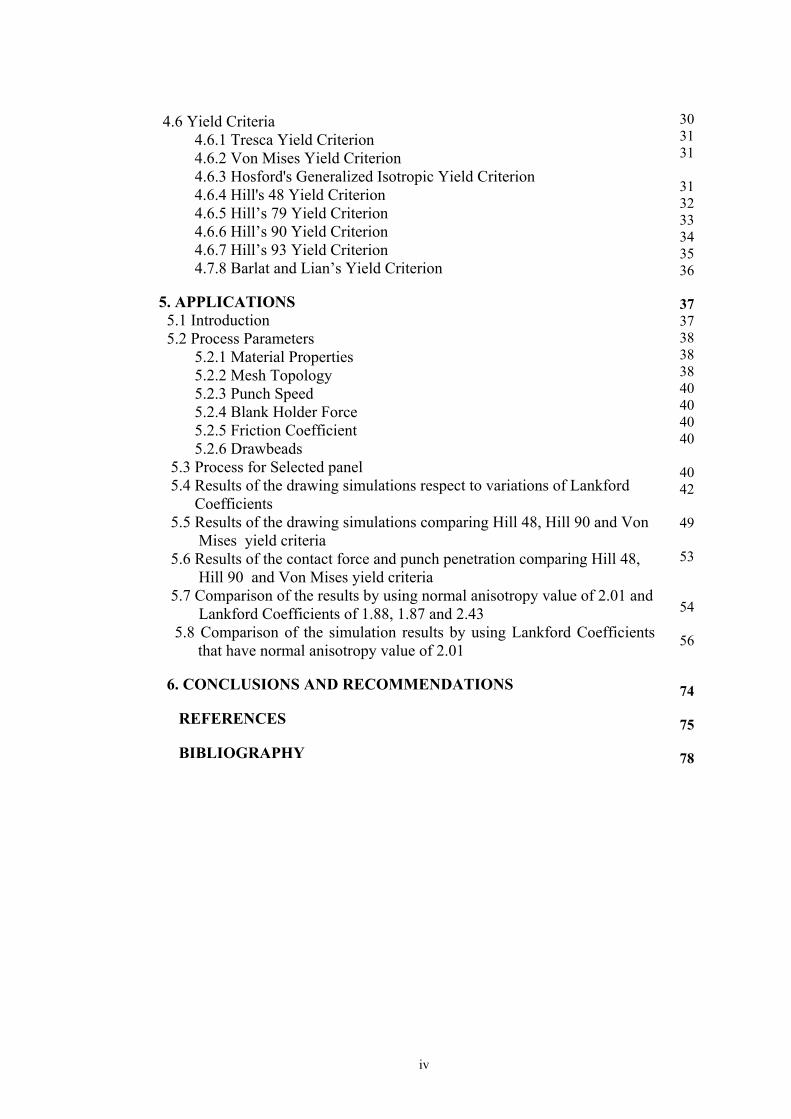
TABLE OF CONTENTS

ABBREVIATIONS LIST OF TABLES LIST OF FIGURES LIST OF SYMBOL ÖZET SUMMARY

1. INTRODUCTION

2. LITERATURE SURVEY 2.1 Introduction 2.2 Deep Drawing 2.3 Flanging 2.4 Trimming 2.5 Restrike 3. FORMABILITY OF SHEET METALS 3.1 Introduction 3.2 Blank Holder 3.3 Drawbeads 3.4 Forming Limit Diagram 3.5 Failures in Sheet Metal Forming Operations 3.5.1 Fracture 3.5.2 Buckling and Wrinkling 3.5.4 Shape Distorsion 3.5.5 Orange Peel and Stretcher-Strain Markings 3.5.6 Springback 3.6 Effect of Properties on Forming 3.6.1 Shape of the true stress-strain curve 3.6.2 Anisotropy 3.6.3 Fracture 3.6.4 Homogeneity 3.6.5 Surface Effects 3.6.6 Damage 3.6.7 Rate Sensivity

4. HARDENING MODELS AND CONSTITUTIVE EQUATIONS 4.1 Introduction 4.2 Isotropy of materials 4.3 Anisotropy of materials 4.4 Strain Rate 4.5 True and Engineering Strains

vvi

viix

xixii

1

2 2

2 5 8 9

1010 11 12 13

16 17 19 20 20 21 22 22 23 23 23 24 24 24

2525 25 26 28 30

iv

4.6 Yield Criteria 4.6.1 Tresca Yield Criterion 4.6.2 Von Mises Yield Criterion 4.6.3 Hosford's Generalized Isotropic Yield Criterion 4.6.4 Hill's 48 Yield Criterion 4.6.5 Hill’s 79 Yield Criterion 4.6.6 Hill’s 90 Yield Criterion 4.6.7 Hill’s 93 Yield Criterion 4.7.8 Barlat and Lian’s Yield Criterion 5. APPLICATIONS 5.1 Introduction 5.2 Process Parameters 5.2.1 Material Properties 5.2.2 Mesh Topology 5.2.3 Punch Speed 5.2.4 Blank Holder Force 5.2.5 Friction Coefficient 5.2.6 Drawbeads 5.3 Process for Selected panel 5.4 Results of the drawing simulations respect to variations of Lankford Coefficients 5.5 Results of the drawing simulations comparing Hill 48, Hill 90 and Von Mises yield criteria 5.6 Results of the contact force and punch penetration comparing Hill 48, Hill 90 and Von Mises yield criteria 5.7 Comparison of the results by using normal anisotropy value of 2.01 and Lankford Coefficients of 1.88, 1.87 and 2.43 5.8 Comparison of the simulation results by using Lankford Coefficients

that have normal anisotropy value of 2.01 6. CONCLUSIONS AND RECOMMENDATIONS

REFERENCES

BIBLIOGRAPHY

30 31 31

31 32 33 34 35 36

37 37 38 38 38 40 40 40 40

40 42

49

53

54

56

74

75

78

v

ABBREVIATIONS

BHF : Blankholder Force CAD : Computer Aided Design FEM : Finite Element Method FEA : Finite Element Analysis FLC : Forming Limit Curve FLD : Forming Limit Diagram FCC : Face Centered Cubic BCC : Body Centered Cubic

vi

LIST OF TABLES

Table 4.1 Hill 90 parameters 34Table 5.1 Properties of the material used for panel 38Table 5.2 Lankford Coefficients of the material 38Table 5.3 Coefficients for Hill 90 Analysis 49Table 5.4 Coefficients for Hill 48 and Von Mises Analyses 50Table 5.5 Lankford Coefficients which were set to obtain normal anisotropy

value of 2.01 57

vii

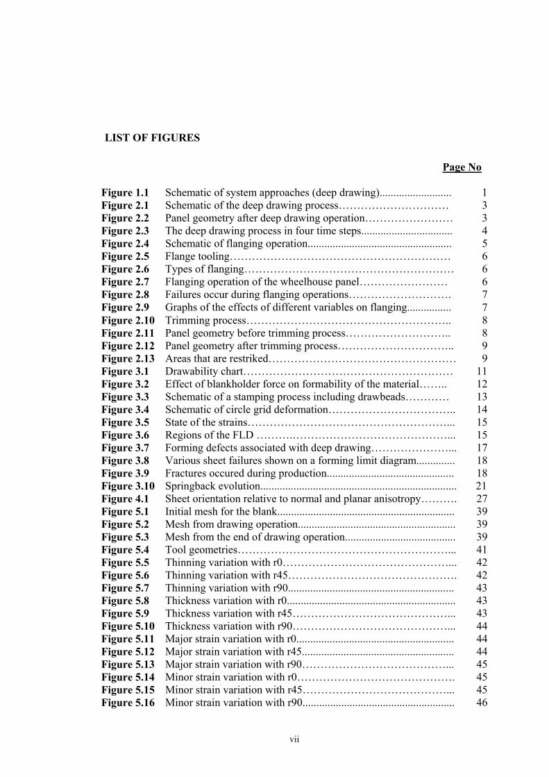
LIST OF FIGURES

Page No

Figure 1.1 Schematic of system approaches (deep drawing).......................... 1Figure 2.1 Schematic of the deep drawing process………………………… 3Figure 2.2 Panel geometry after deep drawing operation…………………… 3Figure 2.3 The deep drawing process in four time steps................................. 4Figure 2.4 Schematic of flanging operation.................................................... 5Figure 2.5 Flange tooling…………………………………………………… 6Figure 2.6 Types of flanging………………………………………………… 6Figure 2.7 Flanging operation of the wheelhouse panel…………………… 6Figure 2.8 Failures occur during flanging operations………………………. 7Figure 2.9 Graphs of the effects of different variables on flanging................ 7Figure 2.10 Trimming process……………………………………………….. 8Figure 2.11 Panel geometry before trimming process……………………….. 8Figure 2.12 Panel geometry after trimming process………………………….. 9Figure 2.13 Areas that are restriked…………………………………………… 9Figure 3.1 Drawability chart………………………………………………… 11Figure 3.2 Effect of blankholder force on formability of the material…….. 12Figure 3.3 Schematic of a stamping process including drawbeads………… 13Figure 3.4 Schematic of circle grid deformation…………………………….. 14Figure 3.5 State of the strains………………………………………………... 15Figure 3.6 Regions of the FLD ……….……………………………………... 15Figure 3.7 Forming defects associated with deep drawing…………………... 17Figure 3.8 Various sheet failures shown on a forming limit diagram.............. 18Figure 3.9 Fractures occured during production.............................................. 18Figure 3.10 Springback evolution....................................................................... 21 Figure 4.1 Sheet orientation relative to normal and planar anisotropy………. 27Figure 5.1 Initial mesh for the blank................................................................ 39Figure 5.2 Mesh from drawing operation......................................................... 39Figure 5.3 Mesh from the end of drawing operation........................................ 39Figure 5.4 Tool geometries…………………………………………………... 41Figure 5.5 Thinning variation with r0………………………………………... 42Figure 5.6 Thinning variation with r45………………………………………. 42Figure 5.7 Thinning variation with r90............................................................ 43Figure 5.8 Thickness variation with r0............................................................. 43Figure 5.9 Thickness variation with r45……………………………………... 43Figure 5.10 Thickness variation with r90……………………………………... 44Figure 5.11 Major strain variation with r0......................................................... 44Figure 5.12 Major strain variation with r45....................................................... 44Figure 5.13 Major strain variation with r90…………………………………... 45Figure 5.14 Minor strain variation with r0……………………………………. 45Figure 5.15 Minor strain variation with r45…………………………………... 45Figure 5.16 Minor strain variation with r90....................................................... 46

viii

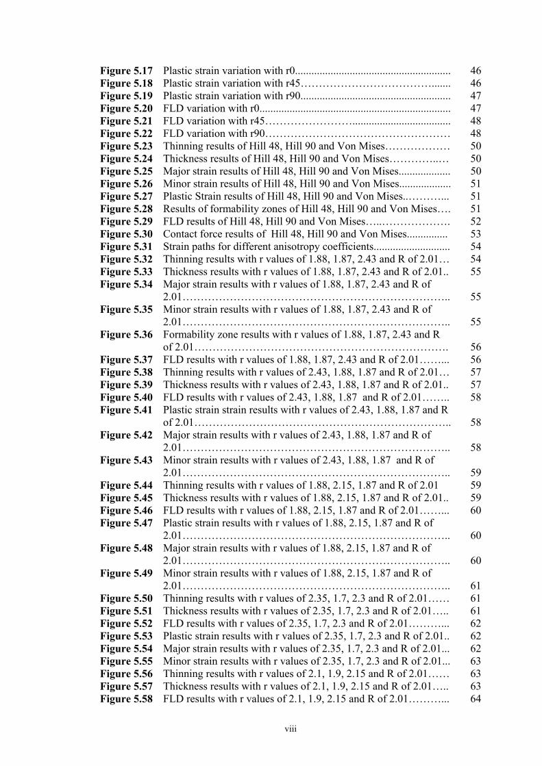
Figure 5.17 Plastic strain variation with r0......................................................... 46Figure 5.18 Plastic strain variation with r45………………………………....... 46Figure 5.19 Plastic strain variation with r90....................................................... 47Figure 5.20 FLD variation with r0...................................................................... 47Figure 5.21 FLD variation with r45…………………….................................... 48Figure 5.22 FLD variation with r90…………………………………………… 48Figure 5.23 Thinning results of Hill 48, Hill 90 and Von Mises……………… 50Figure 5.24 Thickness results of Hill 48, Hill 90 and Von Mises…………..… 50Figure 5.25 Major strain results of Hill 48, Hill 90 and Von Mises................... 50Figure 5.26 Minor strain results of Hill 48, Hill 90 and Von Mises................... 51Figure 5.27 Plastic Strain results of Hill 48, Hill 90 and Von Mises..………... 51Figure 5.28 Results of formability zones of Hill 48, Hill 90 and Von Mises…. 51Figure 5.29 FLD results of Hill 48, Hill 90 and Von Mises…..………………. 52Figure 5.30 Contact force results of Hill 48, Hill 90 and Von Mises............... 53Figure 5.31 Strain paths for different anisotropy coefficients............................ 54Figure 5.32 Thinning results with r values of 1.88, 1.87, 2.43 and R of 2.01… 54Figure 5.33 Thickness results with r values of 1.88, 1.87, 2.43 and R of 2.01.. 55Figure 5.34 Major strain results with r values of 1.88, 1.87, 2.43 and R of

2.01……………………………………………………………….. 55Figure 5.35 Minor strain results with r values of 1.88, 1.87, 2.43 and R of

2.01……………………………………………………………….. 55Figure 5.36 Formability zone results with r values of 1.88, 1.87, 2.43 and R

of 2.01……………………………………………………………. 56Figure 5.37 FLD results with r values of 1.88, 1.87, 2.43 and R of 2.01……... 56Figure 5.38 Thinning results with r values of 2.43, 1.88, 1.87 and R of 2.01… 57Figure 5.39 Thickness results with r values of 2.43, 1.88, 1.87 and R of 2.01.. 57Figure 5.40 FLD results with r values of 2.43, 1.88, 1.87 and R of 2.01…….. 58Figure 5.41 Plastic strain strain results with r values of 2.43, 1.88, 1.87 and R

of 2.01…………………………………………………………….. 58Figure 5.42 Major strain results with r values of 2.43, 1.88, 1.87 and R of

2.01……………………………………………………………….. 58Figure 5.43 Minor strain results with r values of 2.43, 1.88, 1.87 and R of

2.01……………………………………………………………….. 59Figure 5.44 Thinning results with r values of 1.88, 2.15, 1.87 and R of 2.01 59Figure 5.45 Thickness results with r values of 1.88, 2.15, 1.87 and R of 2.01.. 59Figure 5.46 FLD results with r values of 1.88, 2.15, 1.87 and R of 2.01……... 60Figure 5.47 Plastic strain results with r values of 1.88, 2.15, 1.87 and R of

2.01……………………………………………………………….. 60Figure 5.48 Major strain results with r values of 1.88, 2.15, 1.87 and R of

2.01……………………………………………………………….. 60Figure 5.49 Minor strain results with r values of 1.88, 2.15, 1.87 and R of

2.01……………………………………………………………….. 61Figure 5.50 Thinning results with r values of 2.35, 1.7, 2.3 and R of 2.01…… 61Figure 5.51 Thickness results with r values of 2.35, 1.7, 2.3 and R of 2.01….. 61Figure 5.52 FLD results with r values of 2.35, 1.7, 2.3 and R of 2.01………... 62Figure 5.53 Plastic strain results with r values of 2.35, 1.7, 2.3 and R of 2.01.. 62Figure 5.54 Major strain results with r values of 2.35, 1.7, 2.3 and R of 2.01... 62Figure 5.55 Minor strain results with r values of 2.35, 1.7, 2.3 and R of 2.01... 63Figure 5.56 Thinning results with r values of 2.1, 1.9, 2.15 and R of 2.01…… 63Figure 5.57 Thickness results with r values of 2.1, 1.9, 2.15 and R of 2.01….. 63Figure 5.58 FLD results with r values of 2.1, 1.9, 2.15 and R of 2.01………... 64

ix

Figure 5.59 Plastic strain results with r values of 2.1, 1.9, 2.15 and R of 2.01.. 64Figure 5.60 Major strain results with r values of 2.1, 1.9, 2.15 and R of 2.01.. 64Figure 5.61 Minor strain results with r values of 2.1, 1.9, 2.15 and R of 2.01.. 65Figure 5.62 Thinning results with r values of 1.8, 2.1, 2.05 and R of 2.01…… 65Figure 5.63 Thickness results with r values of 1.8, 2.1, 2.05 and R of 2.01….. 65Figure 5.64 FLD results with r values of 1.8, 2.1, 2.05 and R of 2.01……….. 66Figure 5.65 Plastic strain results with r values of 1.8, 2.1, 2.05 and R of 2.01.. 66Figure 5.66 Major strain results with r values of 1.8, 2.1, 2.05 and R of 2.01.. 66Figure 5.67 Minor strain results with r values of 1.8, 2.1, 2.05 and R of 2.01.. 67Figure 5.68 Thinning results with r values of 1, 2.28, 2.5 and R of 2.01……... 67Figure 5.69 Thickness results with r values of 1, 2.28, 2.5 and R of 2.01……. 67Figure 5.70 FLD results with r values of 1, 2.28, 2.5 and R of 2.01………….. 68Figure 5.71 Plastic strain results with r values of 1, 2.28, 2.5 and R of 2.01…. 68Figure 5.72 Major strain results with r values of 1, 2.28, 2.5 and R of 2.01….. 68Figure 5.73 Minor strain results with r values of 1, 2.28, 2.5 and R of 2.01….. 69Figure 5.74 Thinning results with r values of 2.92, 1.1, 2.92 and R of 2.01….. 69Figure 5.75 Thickness results with r values of 2.92, 1.1, 2.92 and R of 2.01... 69Figure 5.76 FLD results with r values of 2.92, 1.1, 2.92 and R of 2.01………. 70Figure 5.77 Plastic strain results with r values of 2.92, 1.1, 2.92 and R of 2.01 70Figure 5.78 Major strain results with r values of 2.92, 1.1, 2.92 and R of 2.01. 70Figure 5.79 Minor strain results with r values of 2.92, 1.1, 2.92 and R of 2.01. 71Figure 5.80 Thinning results with r values of 2.5, 2.28, 1 and R of 2.01……... 71Figure 5.81 Thickness results with r values of 2.5, 2.28, 1 and R of 2.01……. 71Figure 5.82 FLD results with r values of 2.5, 2.28, 1 and R of 2.01………….. 72Figure 5.83 Plastic strain results with r values of 2.5, 2.28, 1 and R of 2.01…. 72Figure 5.84 Major strain results with r values of 2.5, 2.28, 1 and R of 2.01….. 72Figure 5.85 Minor strain results with r values of 2.5, 2.28, 1 and R of 2.01….. 73

x

LIST OF SYMBOLS

E : Young’s modulus F , H, G, N : Hill48 yielding criteria coefficients K : Material strength coefficient m : Strain rate exponent n : Strain hardening exponent r : Plastic strain ratio R : Normal anisotropy coefficient r0 : Lankford coefficient with respect to rolling direction 0 r45 : Lankford coefficient with respect to rolling direction 45 r90 : Lankford coefficient with respect to rolling direction 90 Δr : Earing tendency coefficient t : Sheet thickness e : Engineering strain ε : True strain

wε : Width strain

tε : Thickness strain u : Displacement of the material v : Velocity of the material flow

xv , yv , zv : Flow component in the x direction t : Measure of time

•

xε ,•

yε ,•

zε : Strain rate components

•

xyγ ,•

yzγ ,•

xzγ : Shear strain rate components

σ y : Yield stress −

σ : Effective Stress −

ε : Effective Strain

w : Sheet width μ : Coefficient of friction

xi

SAC METAL ŞEKİLENDİRMEDE ANİSOTROPİNİN ŞEKİLLEDİRİLEBİLME ÜZERİNDEKİ ETKİSİ

ÖZET

Sac şekillendirme simulayonlarının önemi son yıllarda otomotiv endüstrisinin gelişmesine bağlı olarak artmıştır. Üreticiler, zorlaşan piyasa koşullarında rekabetçi güçlerini koruyabilmek amacıyla maliyetleri düşürmek durumundadırlar. Bu amacla işletmeler sonlu elemanlar yöntemlerini, kalıp üretim aşamasından başlayarak deneme sayılarının azaltılması, malzeme kontrolleri, ekipman dayanım kontrolleri gibi uygulamalarda kullanmaktadır. Otomobil panellerinin üretiminde kırışma, yırtılma, aşırı incelme, yüzey bozulması ve geri yaylanma gibi kusurlar oluşur. Bu kusurların giderilmesi amacıyla, kalıp yüzeylerinin geometrisi, sac malzemenin yapılacak işlemler için uygunluğu, sac malzemenin kalıp boşluguna akışı, pot çemberi kuvvetinin ayarlanması, kalıp ve sac malzeme arasındaki sürtünmenin etkisi, süzdürme çubuklarının konumları ve geometrisi gibi durumlar imalat öncesinde simülasyon programları ile tesbit edilir. Bu çalışmada, ticari simülasyon programları kullanılarak bir otomobil tekerlek yuvası panelinin kalıp yüzeylerinin elde edilmesine dolayısıyla kullanılacak panelin elde edilmesine çalışılmıştır. Çalışmanın ikinci bölümünde bu panelin prosesinde önemli olan işlemler ve literatürde gecen bazı genel kavramlar açıklanmıştır. Üçüncü bölümde sac şekillendirmeye etki eden faktörler ve ortaya çıkabilen kusurlar anlatılmış, bazı durumlar işparçamızla örneklendirilmiştir. Dördüncü bölümde matematiksel malzeme yüzey akış bünye denklemleri, izotropi, anizotsopi kavramları ve ilgili temel ifadeler anlatılmıştır. Beşinci bölümde ise, panelin değişik durumlardaki karşılaştırmalı çekme simülasyonları yer almaktadır. Son bölümde ise bu çalışmadan çıkarılabilen sonuçlar ve gelecekte yapılabilecek benzer bir çalışma için düşünülebilecekler anlatılmıştır.

xii

EFFECTS OF ANISOTROPY ON FORMABILITY IN SHEET METAL

FORMING

SUMMARY

In recent years, significance of sheet forming simulations have risen with respect to development of automobile industry. Manufacturers, have to reduce the costs to remain competitive in the compelling market conditions. For this reason, finite element simulations are used for the die making stage to reduce number of try-outs, to make better material selections and controls for endurance limits of the tools. During the manufacturing of automobile panels, failures such as wrinkling, tearing, thinning, surface distortion and springback can be observed. Geometry of die surfaces, material selection, friction between blank and die, blankholder force locations and geometry of the drawbeads are searched with simulation softwares. In this study, commercial simulation software is used to figure out the parameters of the dies for the automobile wheelhouse panel. In the second chapter, literature survey was made for the process of this panel and some general concepts. In the third chapter, the factors and failures that affect formability were observed . In the fourth chapter, information about isotropy, anisotropy, constitution laws and yielding equations were examined. Results of the analyses of the wheelhouse panel are shown in the fifth chapter. Conclusions and recommendations were made in the last chapter.

1

1.INTRODUCTION

Sheet metal forming operations are the common methods for shaping sheet metals

plastically between tools (dies), into desired final configuration. Thus, simple part

geometry is transformed into a complex one, whereby the tools “store” the desired

geometry and impart pressure on the deforming material through tool/material

interface [15].

A sheet metal forming system is composed of all the input variables such as the

blank (geometry and material), the tooling (geometry and material), the conditions at

the tool/material interface, the mechanics of plastic deformation, the equipment used,

the characteristic of the final product and finally the plant environment where the

process is being conducted. The application of the system approach to sheet metal

forming is illustrated in Figure 1.1, as applied to deep drawing. The “systems

approach” in sheet metal forming allow the study of the input/output relationships

and the effects of process variables on product quality and process economics. To

obtain the desired shape and properties in the product, the metal flow should be well

understood and controlled. The direction of flow, the magnitude of deformation, and

the temperature involved greatly influence the properties of formed products. [15]

Figure 1.1: Schematic of system approaches (Deep Drawing)

2

2.LITARATURE SURVEY

2.1 Introduction

In a literature search, one can find many kinds related with sheet metal operations. In

this thesis, a process of wheelhouse panel is examined. In this point of view, applied

operations to obtain the final shape of wheelhouse panel will be taken into

consideration to narrow the literature survey.

2.2 Deep Drawing

For sheet metal forming simulation the most relevant process is deep drawing, which

will be described in the following.

Deep drawing is a sheet metal forming process where a (plane) sheet of metal is

given a double curved shape through drawing, compression and flattening.Examples

of products manufactured with this process are different vessels, body panels for

cars, airplane components, etc. The sheet of metal is placed between the two halves

of the tooling, the die and the binder. The purpose of the die and the binder is to hold

the sheet with enough force (the binder force) to avoid that wrinkles occur. When the

punch is moved down against the surface of the sheet it pushes the sheet down in to

the die and the sheet will start to bend [2, 5].

3

Figure 2.1: Schematic of the deep drawing process

Figure 2.2: Panel geometry after deep drawing operation

A deep drawn wheelhouse panel is seen in figure 2.2. The panel is ready for the

following operations such as trimming, flanging and restrike.

4

As a mostly used process, deep drawing can be explained in four time steps.

Figure 2.3: The deep drawing process in four time steps [2]

The four steps illustrated are as follows:

1. A cut through the tool set up shows the punch, die and metal sheet (or workpiece)

on the binder. The binder is in an uplifted position.

2. The binder and punch is moved downwards. The binder reaches the sheet ahead of

the punch and thereby a pressure, the binder force, is applied on the sheet. Hence the

peripheral parts of the workpiece are kept in place. If the binder is not flat an initial

forming takes place.

3. The punch is now in contact with the sheet and the sheet is drawn through the

opening in the die. It slides over the die radius. As the punch proceeds downwards

the outer radius of the circular workpiece is reduced. In this process the workpiece is

formed through stretching in the drawing direction, accompanied by compression

and flattening in the circular direction.

4. The punch moves back upwards and the formed component is pushed out of the

tool [2].

5

2.3 Flanging

Flanging is a forming operation in which a narrow strip at the edge of a sheet is bent

along a straight or curved line. Compared to plane strain bending, flanging is applied

on the edges of parts, and the flange length is relatively small. As shown in figure

2.4, a typical bend angle in flanging is 90o [5, 17].

During manufacturing, the sheet metal goes through different dies on its way to a

finished product. After deep drawing, the excess metal is usually trimmed off, and

flanged. Flanging is often a strengthening requirement in the design or to provide a

mating surface for subsequent joining operations. During stretch flanging, a tensile

strain is usually imposed on the sheared edge, causing splitting failure in some cases.

Determination of the sheared edge forming limits is usually conducted by stretching

a punched hole, thereby evaluating formability of the sheared edge [5, 22].

Figure 2.4: Schematic of flanging operation

A typical flange tooling is shown in the figure 2.5 below, this tooling includes a die,

pad and a punch. The die should be sufficiently hard to maintain the proper flange

radius, but should also be tough enough to resist corner chipping. The pad applies

pressure to the sheet metal to clamp the part and avoid the part lifting during the

flanging process. The punch forming the outside flange surface may be highly

stressed. Therefore, it is made of hardened tool steel [17].

Flanging

6

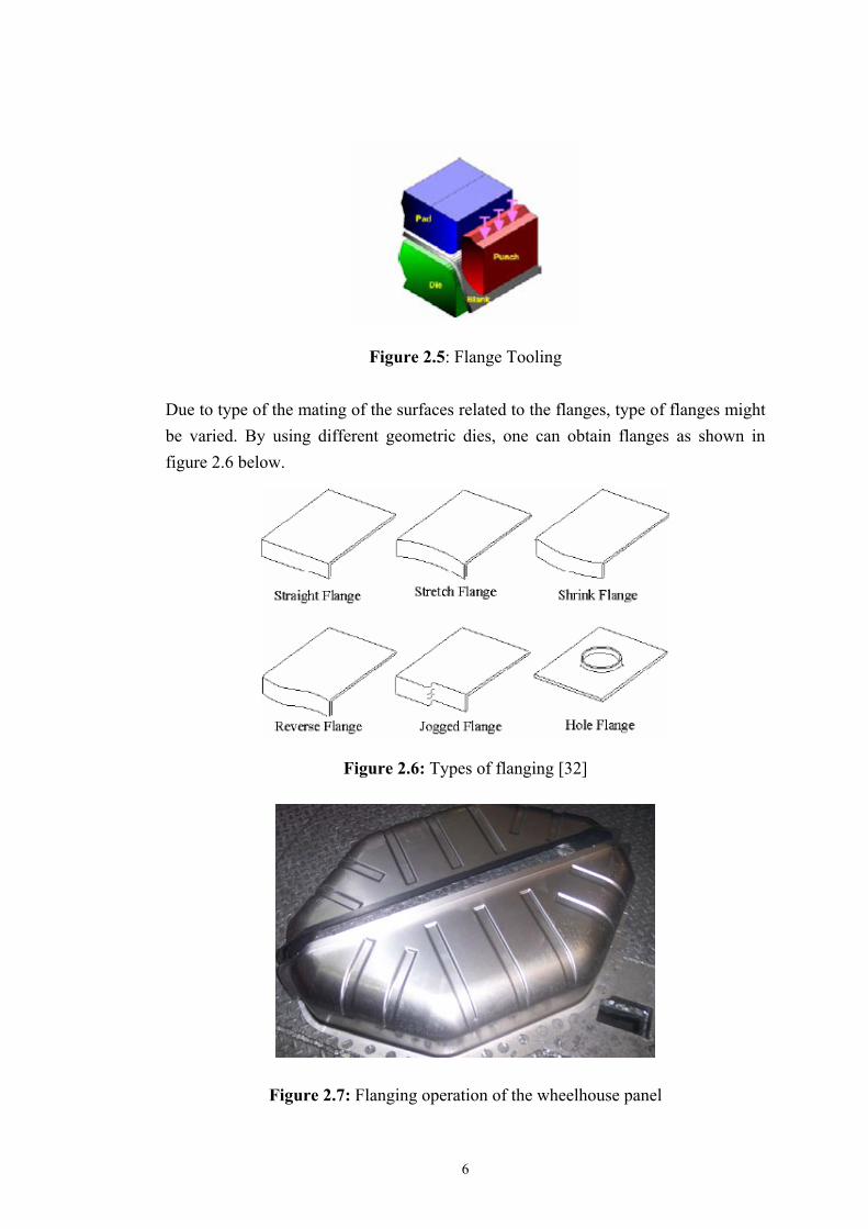
Figure 2.5: Flange Tooling

Due to type of the mating of the surfaces related to the flanges, type of flanges might be varied. By using different geometric dies, one can obtain flanges as shown in figure 2.6 below.

Figure 2.6: Types of flanging [32]

Figure 2.7: Flanging operation of the wheelhouse panel

7

It is important to mention about the failures during the flanging operation.Figure 2.8

shows the major defects of bending and flanging, which are fracture, indenting

folding, necking, wrinkling and calling.

Figure 2.8: Failures occur during flanging operations

The following chart, Figure 2. 9, lists the major flanging variables:

• Die Radius

• Punch Radius

• Clearance Ratio

• Pad Force

And their effects on flanging process:

• Springback

• Die load

• Recoil / Warp

• Minimum Bend Radius (or maximum curvature)

Figure 2.9: Graphs of the effects of different variables on flanging

Necking Wrinkling Calling

8

2.4 Trimming

During any press working operation in which the part must be held in place by the

press, the outer edge of the part, which is the area usually gripped, becomes marked

and scored. Trimming is the cutting off of the excess metal edge. This operation

might be the last to be performed in a progressive die in order to separate the parts

from the strip. Trimming may be performed vertically or horizontally, depending on

the part configuration [5, 20].

Figure 2.10: Trimming process [20]

Figure 2.11: Panel geometry before trimming process

9

Figure 2.12: Panel geometry after trimming process

2.5 Restrike

When the tools are removed away after the operation, internal forces caused the

elastic recovery. This recovery can be observed in the bending, bending-unbending,

reverse bending areas. This is one of the major problems in die making field

because of the aligning and mating problems during the assembly process of the

panels.

This phenomenon is called sprinback and it has to be compansated by overcrowning

and overbending techniques on the die surface. Another technique for the

compansation is the restrike operation. The restrike die hits the areas where

compansation is needed and prepares the panel for the following operations.

Figure 2.13 :Areas that are restriked

10

3. FORMABILITY OF SHEET METALS

3.1 Introduction

The industrial metal working process of sheet metal forming is strongly dependent

on numerous interactive variables: material behaviour, lubrication, forming

equipment etc. One of the main limitations in industrial stampings seems to be the

appearance of localized necking. The mathematical ability to deform plastically

depends on a great number of interactive parameters whose experimental study is a

difficult task. The theoretical analysis of the plastic instability is therefore of major

importance in order to predict the forming limit strains, examine the influence of

each parameter on the necking occurrence and improve press performance. From this

view, forming limit diagram represents a useful concept on sheet metal formability

characterization and very important safety tool in sheet metal forming simulation

which is written in the next section [14, 27].

The quality of a stamped commercial part is largely influenced by the material flow

within the tools during the sheet metal forming operation. Therefore it is important to

control the material flow rate to avoid defects such as wrinkling, tearing, surface

distortion and springback. Furthermore, in car body manufacturing it is important

that outer panels should be subjected to sufficient straining because of the flex

resistance (or dent resistance) [19, 24]. Often, it is desirable to increase material flow

by using lubricants to reduce stress. In other situations, it is common practice to

reduce flow by introducing additional restraining force.

Generally, the material flow is controlled by the blankholder: a restraining force is

created by friction between the tools and the blank. As a result, the tensile stresses

are increased, material flow is controlled, and the formation of wrinkles is avoided.

11

3.2 Blank Holder

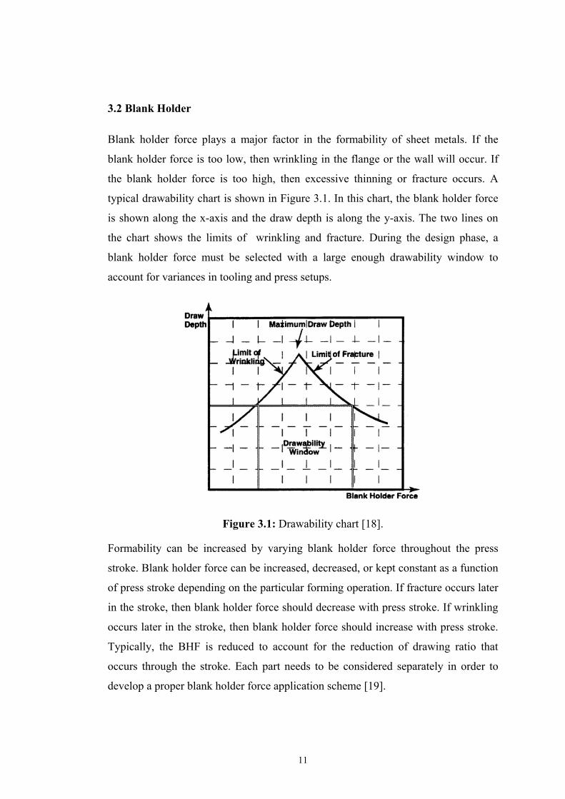
Blank holder force plays a major factor in the formability of sheet metals. If the

blank holder force is too low, then wrinkling in the flange or the wall will occur. If

the blank holder force is too high, then excessive thinning or fracture occurs. A

typical drawability chart is shown in Figure 3.1. In this chart, the blank holder force

is shown along the x-axis and the draw depth is along the y-axis. The two lines on

the chart shows the limits of wrinkling and fracture. During the design phase, a

blank holder force must be selected with a large enough drawability window to

account for variances in tooling and press setups.

Figure 3.1: Drawability chart [18].

Formability can be increased by varying blank holder force throughout the press

stroke. Blank holder force can be increased, decreased, or kept constant as a function

of press stroke depending on the particular forming operation. If fracture occurs later

in the stroke, then blank holder force should decrease with press stroke. If wrinkling

occurs later in the stroke, then blank holder force should increase with press stroke.

Typically, the BHF is reduced to account for the reduction of drawing ratio that

occurs through the stroke. Each part needs to be considered separately in order to

develop a proper blank holder force application scheme [19].

12

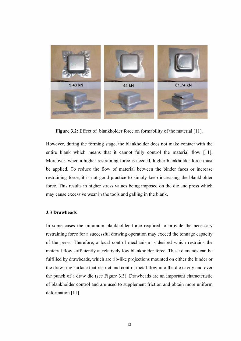
Figure 3.2: Effect of blankholder force on formability of the material [11].

However, during the forming stage, the blankholder does not make contact with the

entire blank which means that it cannot fully control the material flow [11].

Moreover, when a higher restraining force is needed, higher blankholder force must

be applied. To reduce the flow of material between the binder faces or increase

restraining force, it is not good practice to simply keep increasing the blankholder

force. This results in higher stress values being imposed on the die and press which

may cause excessive wear in the tools and galling in the blank.

3.3 Drawbeads

In some cases the minimum blankholder force required to provide the necessary

restraining force for a successful drawing operation may exceed the tonnage capacity

of the press. Therefore, a local control mechanism is desired which restrains the

material flow sufficiently at relatively low blankholder force. These demands can be

fulfilled by drawbeads, which are rib-like projections mounted on either the binder or

the draw ring surface that restrict and control metal flow into the die cavity and over

the punch of a draw die (see Figure 3.3). Drawbeads are an important characteristic

of blankholder control and are used to supplement friction and obtain more uniform

deformation [11].

13

Figure 3.3: Schematic of a stamping process including drawbeads [11].

3.4 Forming Limit Diagram

In all sheet metal forming operations, one has to care about the state of the blank

until the final shape is obtained. Using forming limit diagrams are the most

convenient way to avoid failures in the operations. The forming limit diagram offers

the chance to determine process limitations in sheet metal forming and it is used in

the estimation of stamping characteristics of sheet metal materials. The FLD is

usually applied in method planning method planning, in tool construction and in tool

shops for optimizing stamping tools and their geometries. With the help of the form

modification analysis and the comparison with the FLD, an optimisation of the

parameters that influence stamping process such as tool geometries, press pad

pressure, lubrication, material will result. A further important area for FLD is in the

field of numerical simulations of transformation processes. The FLD of the used

material is a necessary prerequisite for the estimation of the simulation results [6].

The early work of Keeler and Backofen (1963) showed that a critical combination of

major and minor strains would lead to localized necking. The work of both Keeler

and Goodwin (1968) led to the construction of a FLC in principal strain space where

14

any combination of strains above the curve presents some probability of failure (i.e.

necking or splitting). formability of sheet materials. Some examples of this research

include attempting to identify the optimum method for constructing the FLC,

developing a theoretical framework for predicting strain localization and studying the

effects of strain path on the FLC. However, the biggest impact of the FLC has been

in the press shop [6,10,28].

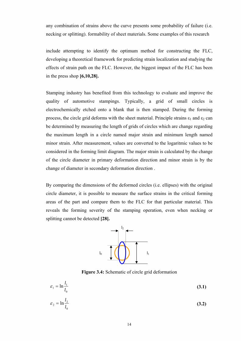
Stamping industry has benefited from this technology to evaluate and improve the

quality of automotive stampings. Typically, a grid of small circles is

electrochemically etched onto a blank that is then stamped. During the forming

process, the circle grid deforms with the sheet material. Principle strains ε1 and ε2 can

be determined by measuring the length of grids of circles which are change regarding

the maximum length in a circle named major strain and minimum length named

minor strain. After measurement, values are converted to the logaritmic values to be

considered in the forming limit diagram. The major strain is calculated by the change

of the circle diameter in primary deformation direction and minor strain is by the

change of diameter in secondary deformation direction .

By comparing the dimensions of the deformed circles (i.e. ellipses) with the original

circle diameter, it is possible to measure the surface strains in the critical forming

areas of the part and compare them to the FLC for that particular material. This

reveals the forming severity of the stamping operation, even when necking or

splitting cannot be detected [28].

Figure 3.4: Schematic of circle grid deformation

0

11 ln

ll

=ε (3.1)

0

22 ln

ll

=ε (3.2)

l1

l2

l0

15

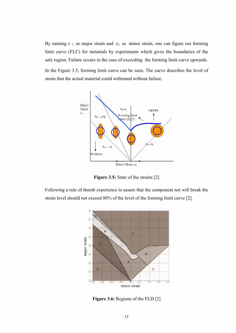
By naming ε 1 as major strain and ε2 as minor strain, one can figure out forming

limit curve (FLC) for metarials by experiments which gives the boundaries of the

safe region. Failure occurs in the case of exceeding the forming limit curve upwards.

In the Figure 3.5, forming limit curve can be seen. The curve describes the level of

strain that the actual material could withstand without failure.

Figure 3.5: State of the strains [2]

Following a rule of thumb experience to assure that the component not will break the

strain level should not exceed 80% of the level of the forming limit curve [2].

Figure 3.6: Regions of the FLD [2]

16

Indicated areas in the figure 3.6 help to determine the state of the component after

forming operation or operations are made [2].

A. Recommended!. Safe region, appropriate use of the forming abilities of the material

B. Danger of rupture or cracking.

C. The material has cracked.

D. Severe thinning.

E. Insufficient plastic strain, risk of spring back

F. Tendency to wrinkling.

G. Fully developed wrinkles (or thickening).

In general, forming limit diagram inspections made with hand made calculations, but

recently, development of image processing technologies and high resolution cameras

help to do this analyses by computer programs. However, general concept of

inspection does not change.

3.5 Failures in sheet metal forming operations

There are potential formability problems typically associated with each forming

operation. The major problems are fracture, buckling and wrinkling, shape distortion,

and undesirable surface textures. It is important to recognize and understand which

defects are associated with a given process and their effects on the finished

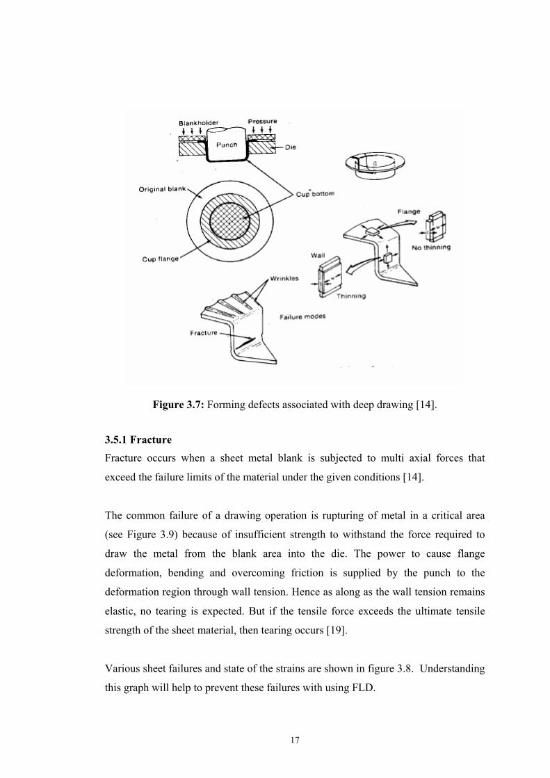
workpiece. Not all failures are purely functional (see figure 3.7). Some defects, such

as stretcher-strains, may not affect the functionality of the part but may make the part

unusable due to aesthetic considerations [14].

17

Figure 3.7: Forming defects associated with deep drawing [14].

3.5.1 Fracture Fracture occurs when a sheet metal blank is subjected to multi axial forces that

exceed the failure limits of the material under the given conditions [14].

The common failure of a drawing operation is rupturing of metal in a critical area

(see Figure 3.9) because of insufficient strength to withstand the force required to

draw the metal from the blank area into the die. The power to cause flange

deformation, bending and overcoming friction is supplied by the punch to the

deformation region through wall tension. Hence as along as the wall tension remains

elastic, no tearing is expected. But if the tensile force exceeds the ultimate tensile

strength of the sheet material, then tearing occurs [19].

Various sheet failures and state of the strains are shown in figure 3.8. Understanding

this graph will help to prevent these failures with using FLD.

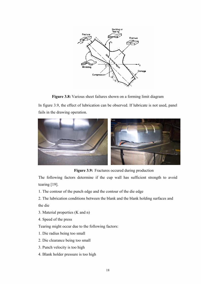
18

Figure 3.8: Various sheet failures shown on a forming limit diagram

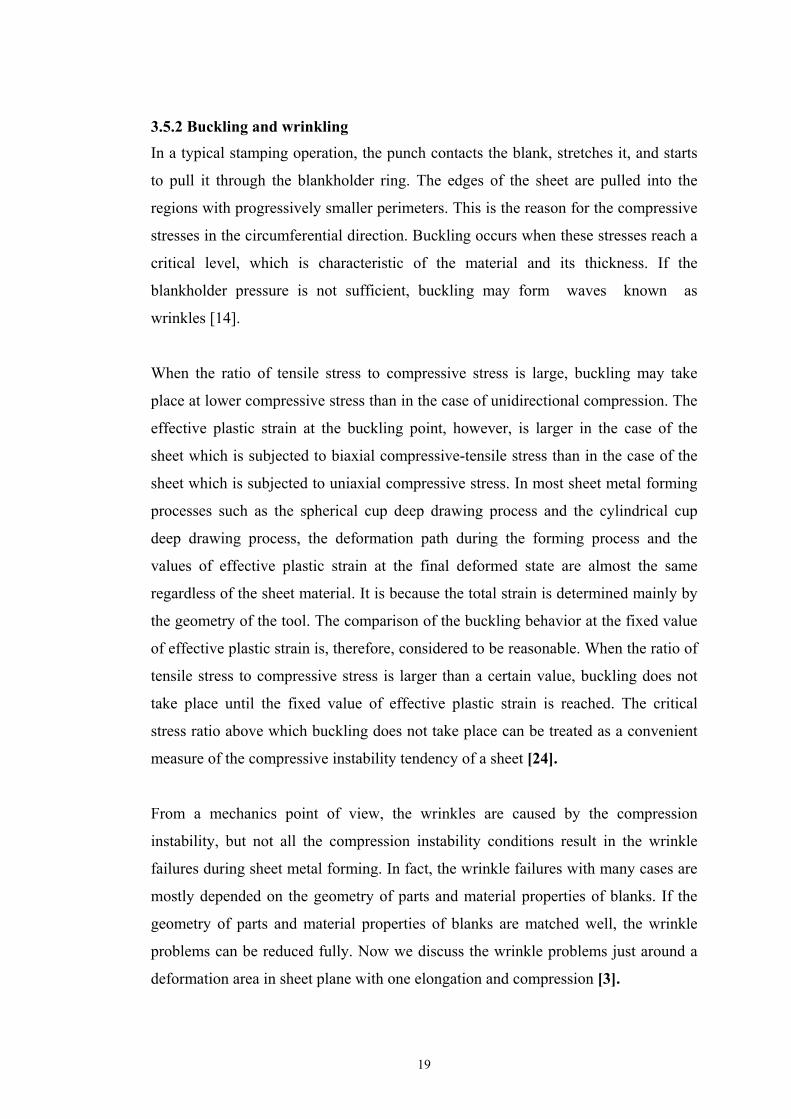
In figure 3.9, the effect of lubrication can be observed. If lubricate is not used, panel

fails in the drawing operation.

Figure 3.9: Fractures occured during production

The following factors determine if the cup wall has sufficient strength to avoid

tearing [19].

1. The contour of the punch edge and the contour of the die edge

2. The lubrication conditions between the blank and the blank holding surfaces and

the die

3. Material properties (K and n)

4. Speed of the press

Tearing might occur due to the following factors:

1. Die radius being too small

2. Die clearance being too small

3. Punch velocity is too high

4. Blank holder pressure is too high

19

3.5.2 Buckling and wrinkling In a typical stamping operation, the punch contacts the blank, stretches it, and starts

to pull it through the blankholder ring. The edges of the sheet are pulled into the

regions with progressively smaller perimeters. This is the reason for the compressive

stresses in the circumferential direction. Buckling occurs when these stresses reach a

critical level, which is characteristic of the material and its thickness. If the

blankholder pressure is not sufficient, buckling may form waves known as

wrinkles [14].

When the ratio of tensile stress to compressive stress is large, buckling may take

place at lower compressive stress than in the case of unidirectional compression. The

effective plastic strain at the buckling point, however, is larger in the case of the

sheet which is subjected to biaxial compressive-tensile stress than in the case of the

sheet which is subjected to uniaxial compressive stress. In most sheet metal forming

processes such as the spherical cup deep drawing process and the cylindrical cup

deep drawing process, the deformation path during the forming process and the

values of effective plastic strain at the final deformed state are almost the same

regardless of the sheet material. It is because the total strain is determined mainly by

the geometry of the tool. The comparison of the buckling behavior at the fixed value

of effective plastic strain is, therefore, considered to be reasonable. When the ratio of

tensile stress to compressive stress is larger than a certain value, buckling does not

take place until the fixed value of effective plastic strain is reached. The critical

stress ratio above which buckling does not take place can be treated as a convenient

measure of the compressive instability tendency of a sheet [24].

From a mechanics point of view, the wrinkles are caused by the compression

instability, but not all the compression instability conditions result in the wrinkle

failures during sheet metal forming. In fact, the wrinkle failures with many cases are

mostly depended on the geometry of parts and material properties of blanks. If the

geometry of parts and material properties of blanks are matched well, the wrinkle

problems can be reduced fully. Now we discuss the wrinkle problems just around a

deformation area in sheet plane with one elongation and compression [3].

20

Wrinkling may be a serious obstacle to implementing the forming process and

assembling the parts, and may also play a significant role in the wear of the tool. In

order to improve the productivity and quality of products, the wrinkling problem

must be solved. At present, sheet metal forming processes are widely used in various

industrial sectors such as automotive, electric home appliance, and aircraft industries.

Also, the needs for high precision and high value-added products are increased. In

order to reduce the process development time, the prediction of defects and the

modification of design in the design stage are needed [24].

3.5.3 Shape Distorsion It occurs when the residual stresses on the outer surfaces are different from those on

the inner surfaces. When these stresses are not compensated by the geometry of the

part, relaxation will cause a change in the part shape known as shape distortion [14].

Residual stresses may also cause geometric distortions in the part. Large-scale

distortions may take the form of highs or lows in the part surface or as oil canning

(elastic instabilities). Small scale distortions may take the form of rabbit earing, pie

crust, crow’s feet, or teddy bear ears [19].

3.5.4 Orange Peels and Stretcher-Strain Markings

During the stretching of some metals, especially aluminum-magnesium alloys and

some low carbon steels, visible localized yielding, called stretcher-strain markings,

occur. They are extremely undesirable because of their negative influence on the

surface quality of the parts. Painting cannot usually conceal this highly visible

phenomenon. Therefore, these sheets cannot be used as outer auto body panels [14].

Undesirable surface textures such as orange peel or stretcher strain markings may

also occur during deformation. Orange peel consists of a rough surface appearance

typically caused by the variation of flow stress properties of the various grains

contained in the material. Two types of stretcher strains are observed. The first type

is caused by discontinuous yielding at the yield point and is evidenced by irregular

striations on the surface of the sheet. The second type of stretcher strain marking is

caused by discontinuous yielding in the plastic region of the material and is

evidenced by regular striations on the surface of the sheet [19].

21

3.5.5 Springback

In addition to the formability concerns, sprinback is another significant problem that

must be solved in order to form the exact shape of the product.Sprinback is a

common phenomenon in sheet metal forming and can be affected by various

parameters such as material properties, tooling geometry,friction between the sheet

metal and the tooling,blank holder force,etc.As soon as the deformed part removed

from the die cavity, springback occurs,espicially where bending,unbending and

bending-unbending-reverse bending are performed. Change in shape that caused by

sprinback introduces problems in assebly process, so die makers must allow for the

sprinback before having troubles [4].

Finite element method takes place again in order to predict sprinback in the die

design stage. General tendency on springback phenomenon is passing a little work to

do for the tool operators who are finalize the die making job. In this view, experince

and knowledge of the FEM user is very significant here. Considering which

hardening rule is accounted for, yielding criteria selected, behaviours of the materials

and which operations will be applied during the process help the work to do easier.

Figure 3.10: Springback evolution

Furthermore, the accuracy of this unloading bending moment depends on the internal

stress distribution within the sheet metal element.In other words, it is not possible to

obtain an accurate sprinback prediction with a rough internal stress disribution. Most

of the sheet materials undergo complicated deformation histories during the forming

process.This means that the Bauschinger effect exists within these elements since

they may have one or more reverse yields. Therefore, The Bauschinger effect has to

be considered for obtaining an accurate internal stress distribution within the sheet

metal [4].

22

3.6 Effects of Properties on Forming

It is found that the way in which a given sheet behaves in a forming process will

depend on one or more general characteristics. Which of these is important will

depend on the particular process and by studying the mechanics equations governing

the process it is often possible to predict those properties that will be important. This

assumes that the property has a fundamental significance, but, not all the properties

obtained from the tensile test will fall into this category. The general attributes of

material behaviour that affect sheet metal forming are as follows [1].

3.6.1 Shape of the true stress-strain curve

The important aspect is strain-hardening. The greater the strain-hardening of the

sheet, the better it will perform in processes where there is considerable stretching;

the straining will be more uniformly distributed and the sheet will resist tearing when

strain-hardening is high. There are a number of indicators of strain-hardening and the

strain-hardening index, n, is the most precise. Other measures are the tensile/yield

ratio, the total elongation, and the maximum uniform strain, the higher these are, the

greater is the strain-hardening.

The importance of the initial yield strength, is related to the strength of the formed

part and particularly where lightweight construction is desired, the higher the yield

strength, the more efficient is the material. Yield strength does not directly affect

forming behaviour, although usually higher strength sheet is more difficult to form.

This is because of other properties change in an adverse manner as the strength

increases. The elastic modulus also affects the performance of the formed part and a

higher modulus will give a stiffer component, which is usually an advantage. In

terms of forming, the modulus will affect the springback. A lower modulus gives a

larger springback and usually more difficulty in controlling the final dimensions. In

many cases, the springback will increase with the ratio of yield stress to modulus,

and higher strength sheet will also have greater springback [1].

23

3.6.2 Anisotropy

If the magnitude of the planar anisotropy parameter, ΔR, is large, either, positive or

negative, the orientation of the sheet with respect to the die or the part to be formed

will be important; in circular parts, asymmetric forming and earing will be observed.

If the normal anisotropy ratio R is greater than unity it indicates that in the tensile

test the width strain is greater than the thickness strain; this may be associated with a

greater strength in the through-thickness direction and, generally, a resistance to

thinning. Normal anisotropy R also has more subtle effects. In drawing deep parts, a

high value allows deeper parts to be drawn. In shallow, smoothly-contoured parts

such as autobody outer panels, a higher value of R may reduce the chance of

wrinkling or ripples in the part. Other factors such as inclusions, surface topography,

or fracture properties may also vary with orientation; these would not be indicated by

the R- value which is determined from plastic properties [1, 14].

3.6.3 Fracture

Even in ductile materials, tensile processes can be limited by sudden fracture. The

fracture characteristic is not given by total elongation but is indicated by the cross-

sectional area of the fracture surface after the test-piece has necked and failed. This is

difficult to measure in thin sheet and consequently problems due to fracture may not

be properly recognized [1].

3.6.4 Homogeneity

Industrial sheet metal is never entirely homogeneous, nor free from local defects.

Defects may be due to variations in composition, texture or thickness, or exist as

point defects such as inclusions. These are difficult to characterize precisely.

Inhomogeneity is not indicated by a single tensile test and even with repeated tests,

the actual volume of material being tested is small, and non-uniformities may not be

adequately identified [1].

24

3.6.5 Surface Effects

The roughness of sheet and its interaction with lubricants and tooling surfaces will

affect performance in a forming operation, but will not be measured in the tensile

test. Special tests exist to explore surface properties [1].

3.6.6 Damage

During tensile plastic deformation, many materials suffer damage at the

microstructural level. The rate at which this damage progresses varies greatly with

different materials. It may be indicated by a diminution in strain-hardening in the

tensile test, but as the rate of damage accumulation depends on the stress state in the

process, tensile data may not be indicative of damage in other stress states [1].

3.6.7 Rate Sensivity

The rate sensitivity of most sheet is small at room temperature; for steel it is slightly

positive and for aluminium, zero or slightly negative. Positive rate sensitivity usually

improves forming and has an effect similar to strain-hardening. As well as being

indicated by the exponent m, it is also shown by the amount of extension in the

tensile test-piece after maximum load and necking and before failure [1].

25

4. HARDENING MODELS AND CONSTITUTIVE EQUATIONS

4.1 Introduction

Sheet metal forming is a difficult job that makes the engineers and operators to

struggle until the desired part is obtained. Sheet metal processes involve design

stage, material selections, forming simulations using computer codes or commercial

softwares which are said to be die design, blank design, stamping, trimming, flanging

simulations etc. These processes continue with the try-outs until the dimensions of

the part remain in the specified tolerances. All these operations can go up to the time

interval of 12 – 15 months.

It is obvious that any mistake in these time-consuming operations cause loss of

money for die makers and patience and confident of the customer.

As a result, the parameters have great importance which are used in simulations for

predicting exact data with minimum time and material loss.

In this section, one can find the basic concepts of sheet metal forming and also some

critical points which engineers must pay attention about the usage of yielding

criteria.

4.2 Isotropy Of The Materials

A metal, in its generally used form, is a compact aggregate of crystal grains with

varying shapes and orientation, each grain having grown from a separate nucleus in

the melt. The metal may be considered macroscopically isotropic when the

orientations are randomly distributed and when the average dimensions of the

individual crystals are small compared with the dimensions of whole specimen.

Nevertheless the properties of an aggregate are not always simply statistical averages

of the properties of a single crystal, taken over all orientations. While this is

approximately true of properties which depend mainly on the bulk structure, such as

26

the coefficient of thermal expansion or the elastic moduli, it is not necessarily true of

the plastic phenomena [7].

Shortly, If there is no difference in the metal’s microstructure in all directions, the

metal is said to be isotropic.

4.3 Anisotropy Of The Materials

The microstructure of metallic materials can be either isotropic or anisotropic. This

means that the microstructure can be either constant in all directions or be aligned in

a certain direction. If the metal has any pattern or alignment of its microstructure, it

is said to be anisotropic. Anisotropy is considered in two forms; normal and planar.

Normal anisotropy measures the change in material characteristics, which differ

through the thickness of the sheet, while planar anisotropy measures material

characteristic differences in various directions within the plane of the sheet. Figure

4.1 defines normal and planar anisotropy relative to the sheet [14].

The microstructure of the metal can have great impact on the ability of the metal to

be formed into the desired shape. A prevalent cause for planar anisotropy in sheet

metals is the rolling direction. During processing of sheet metal, the rolling operation

elongates and aligns the grains of the metal’s microstructure in the rolling direction

and packs the grains in the thickness direction, which leads to significantly different

strength properties within the material.

The internal stress state at the end of forming depends on the plastic properties of the

material and their evolution during forming. Cold-rolling induces preferred

orientation of polycrystalline grains, and the texture-induced anisotropy can be

assessed by measured plastic anisotropy parameters related to strains (r-values) or

flow stresses, or can be predicted from texture measurements using simple averaging

rules [21].

During a tensile test, the width of the material and the thickness decrease as the

elongation increases. The plastic strain ration, r, is the ratio of width strain to

thickness strain.

27

t

wrεε

= (4.1)

Where wε is the width strain and tε is the thickness strain. This ratio is useful for

determining the degree of anisotropy in the material and rating its resistance to

thinning. If the ratio is equal to one, then the material is isotropic, since the strain is

equal in both thickness and width. The r ratio values are a measure of the drawability

of the sheet metal [16].

For high strain ratios, the material is said to be resistant to thinning, while materials

with low strain ratios will be undesirable for forming operations, since it will thin

and possibly rupture.

Figure 4.1: Sheet orientation relative to normal and planar anisotropy [14].

The strain ratio is determined relative to the rolling direction of the sheet material,

thus r0 (parallel), r45 (diagonal) and r90 (transverse) can be determined through

geometry. The plastic anisotropy coefficients are assessed by the means of plastic

strain ratios of these three planes which are also called as Lankford coefficients. The

weighted average, R, of these strain ratios, which is also called normal anisotropy is

defined as

4

2 90450 rrrR

++= (4.2)

The directional strain ratio measures are useful for determining the earing tendency

of the material, Δr [14, 25].

Rolling direction

Normal Anisotropy R

r00

r 45

0

r 900

Planar Anisotropy Δr

28

2

2 90450 rrrr

+−=Δ (4.3)

Where Δr is the earing tendency, r0, r45, and r90 are the strain ratios. The Earing

tendency is simply the likelihood that the sheet will draw non uniformly and form

ears in the flange [14].

4.4 Strain Rate

During deformation, material flow is rarely uniform in all directions and regions. The

velocity of the metal flow depends on the geometry of the die, strain hardening,

temperature, material microstructure, anisotropy, and applied loading rate.

The velocity of metal flow is described as

tuv

∂∂

= (4.4)

Where ν is the deformation velocity, u is the displacement of material, and t is a

measure of time. Metal flow is not necessarily the same in all directions within the

material, thus, flow velocity has directional components νx, νy, and νz

t

uv x

x ∂∂

= , t

uv y

y ∂

∂= ,

tuv z

z ∂∂

= (4.5)

Strain rate is defined as the change in strain with respect to time. Since strain is

dependent on the deformation of the material with respect to distance, strain rate can

be defined as the change in metal flow with respect to change in location [14].

xv

tu

xxu

ttx

xxxx

x ∂∂

=⇒∂

∂∂∂

=∂

∂∂∂

=∂

∂=

••

εε

ε (4.6)

Where •

xε is the strain rate, u is the deformation of material, v is the deformation

velocity and t is a measure of time. The strain rate values in the other directions, are

derived in a similar manner.

yvy

y ∂

∂=

•

ε (4.7)

zvz

z ∂∂

=•

ε (4.8)

Shear strain rate is defined as

xv

yv yx

xy ∂

∂+

∂∂

=•

γ (4.9)

29

Where •

xyγ is the shear strain rate and v is the deformation velocity. As with normal

strain rate, shear strain rate has components •

yzγ and •

xzγ defined similar to •

xyγ .

yv

zv zy

yz ∂∂

+∂

∂=

•

γ (4.10)

xv

zv zx

xz ∂∂

+∂∂

=•

γ (4.11)

The state of deformation in a plastically deforming metal can be fully described by

the displacements, u, velocities, v, strains, ε, and strain rates, •

ε . These values can be

defined in an auxiliary coordinate system (x’,y’,z’) if the angle of rotation form the

global coordinate system (x,y,z) is known. Thus, a small element in the deforming

body can be oriented such that it is not subjected to shear. With this definition, the

shear strains, γxy, γyz and γxz, equal zero and the element deforms along the principle

axes. This representation of deformation corresponds with the results of uniaxial

tension tests, since they also deform in the principal direction.

The assumption of volume constancy neglects elastic strain when the relative plastic

strain is much greater. This assumption can also be expressed, for deformation along

principle axes, as follows:

0=++ zyx εεε (4.12)

0=++•••

zyx εεε (4.13)

Strain and strain rate, along with temperature, affect the magnitude of the flow. This

relationship is usually dependent on the direction of the strain (anisotropy), because

the properties of a sheet material (i.e. flow stress as a function of strain, strain rate,

and temperature) depend on the rolling direction.

30

4.5 True and Engineering Strains

Strength of materials theory defines engineering strain as deformation with respect to

the initial length, thus:

0

0

λ

λλ −= fe (4.14)

where e is the engineering strain, fλ is the deformed length and 0λ is the original

length. This measure of strain is useful for design, since it is very easy to calculate.

Engineering strain is not accurate for large deformations, however for design

purposes, the component is assumed to deform very little, so this measure provides

useful results [14].

For large deformations, more accurate measure of deformation is true strain, which

relates the change in length to instantaneous unit length. Instantaneous true strain is

defined as:

⎟⎟⎠

⎞⎜⎜⎝

⎛== ∫

0

ln0

λ

λ

λλ

λ

λ

ff dε (4.15)

where ε is the true strain, fλ is the deformed length, and 0λ is the original unit

length. This measure provides the exact value of strain, taking into account the

effects of dimensional change. True strain is useful when large deformations occur,

such as forming operations thus it is commonly used for process design.

Engineering and true strains are related by the following equation

( )1ln += eε (4.16)

This equation provides an easy conversion from engineering to true strain depending

on available information.

4.6 Yield Criteria

The analysis of localized necking is strongly dependent on the yield function. Since

the geometric configuration of the yield surface has a significant influence on

predicted forming limit strains, many yield criteria have been proposed to reflect the

material properties of sheet metals. Usage of these criteria are vary with different

31

kinds of materials and different loading conditions. By these considerations, better

simulation results will be obtained.

The common yield criteria are listed below:

4.6.1 Tresca Criterion

Based on Coulomb’s results on soil mechanics and his own experiments results on

the metal extrusion, Tresca (1864) proposed a yield criterion, and this criterion can

be expressed as

kMax =⎥⎦⎤

⎢⎣⎡ −−− 313221 2

1,21,

21 σσσσσσ (4.17)

Where k value can be determined by the uniaxial test, and its value is equal to a half

of the yield stress.

4.6.2 Von Mises Yield Criterion

Von Mises (1913) yield criterion, which can also be called a J2 criterion, can be

written as:

( ) ( ) ( ) 2213

232

221 2 yσσσσσσσ =−+−+−

(4.18)

2

32

yijij SS σ= (4.19)

Where Sij and σ y are the deviatoric stress tensor and yield stress, respectively.

4.6.3 Hosford's Generalized Isotropic Yield Criterion

Hershey (1954) and Hosford (1972) proposed the generalized isotropic yield

criterion based on the results of polycrystalline calculations. The formulation is

expressed in principal stresses, and high order exponents are found to be crystal

structure-related typically 6 for BCC and 8 for FCC metals [23] which is shown in

the equation 4.20.

32

( ) ( ) ( )Y

MMMM

=⎥⎥⎦

⎤

⎢⎢⎣

⎡ −+−+−/1

313221

2σσσσσσ

(4.20)

Where ( )321 σσσ ≥≥ and ( )∞≤≤ M1 is proposed

When M = l, the above equation becomes Tresca criterion, and becomes Von

Mises criterion if M = 2. Because it repeats its shape at lower values when

M > 2.767, the above equation becomes Tresca and Von Mises criteria when

M = ∞ and 4 respectively [4].

Hosford later modified the formula for plane stress conditions and tried to

accommodate shear stresses [23, 27].

4.6.4 Hill's 48 Yield Criterion

Hill proposed several yield criterials which are used for different materials and

different situations.Theory of Hill (1948-1950) describes a state of simple orthotropic

anisotropy, that is, where there are three mutually orthogonal planes of symmetry at

every point. The intersections of these planes are known as the principal axes of

anisotropy [13, 29].

( ) ( ) ( ) ( )122

2222

2222

=++

+−+−+−=

xyzx

yzyxxzzyij

NM

LHGFf

ττ

τσσσσσσσ (4.21)

The coefficients of F, G, H, N are calculated by r0, r 45, r 90 are the tensile test strain

ratios in rolling, diagonal and transverse directions, respectively [12].

( )090

0

1 RRR

F+

= (4.22)

011R

G+

= (4.23)

0

0

1 RR

H+

= (4.24)

33

( )( )( )090

45900

1221

RRRRR

N+

++= (4.25)

For sheet metal forming process, plane stress assumption is adopted and the above

equation can be simplified by setting [4]

0=== yzxyz σσσ (4.26)

Recalling −

R is normal anisotropy from equation 4.2, equation 4.26 can be rewritten

by considering sheet metal forming and assuming that the sheet has planar isotropy

where uσ is the in-plane uniaxial tensile stress [8].

( ) uRR−−−

⎟⎠⎞

⎜⎝⎛ +=−++ 22

2122

12 1 σσσσσ (4.27)

Hill’s quadratic yield function has been used in various analyses of metal forming

processes to account for polycrystalline texture.It is formulated in a general stress

state, and needs only uniaxial tensile tests to describe planar anisotropy. Hovewer, it

is not very suitable for FCC metals exhibiting low R-values, such as aluminum alloy

sheets [23].

In the application chapter, the effect of R-values shown using Hill48 yield criteria.

4.6.5 Hill’s 79 Criterion

For aluminum sheet, the r-value is normally less than unity (between 0.6 and 0.8).

Experimental data show that for most aluminum sheet the yield stress for balanced

biaxial tension is larger than the yield stress for uniaxial tension (anomalous

behavior). Therefore, eq. (4.37) contradicts the physical phenomenon of aluminum

sheets. This indicates that the 1948 criterion may encounter problems when

predicting forming limits of aluminum. In order to deal with the anomaly, Hill

proposed the second yield criterion in 1979 which is a generalization of the Logan

and Hosford yield Criterion [8, 9, 27].

mMM

Mmmm

CB

AHGF

σσσσσσσ

σσσσσσσσσ

222

2

213132

321211332

=−−+−−+

−−+−+−+− (4.28)

34

There are 7 parameters in eq. (4.28). They are determined by uniaxial tension test in

the three orthotropic directions, together with three transverse strain ratios, plus 1

other combined loading test (such as the biaxial tension test). For in-plane isotropy,

the four simple forms of eq. (4.29) were given by Hill and the yield locus of the

fourth equation remains convex as long as the exponent M is greater than unity

Using both uniaxial tension yield stress uσ and r-value, the fourth equation becomes

as below [8]. M

uMM rr σσσσσ )1(2)21( 2121 +=−+++ (4.29)

Calculation of M value is made by fitting of work hardening curves for equi-biaxial

stretching calculated on the base of experimentally determined work hardening

curves in tensile test to experimentally determined work hardening curves in

equibiaxial stretching. It is well knowthat the Hill’79 can model the Woodthorpe–

Pearce “anomalous” behavior of some materials but the main disadvantage is that it

is expressed using only principal stress and the predicted yield surfaces are

sometimes far from the experimental surfaces predicted by the Bishop–Hill

theory [6].

4.6.6 Hill’s 1990 Yield Criterion

Hill’s 90 Criterion Coefficients: are α, β, γ and m. The anisotropic elasto-plastic

plane stress formulation of shell material type is based on a non-quadratic yield

function (Hill 1990), as opposed to a quadratic yield function (Hill 1948). For plane

stress conditions and in the orthotropic axes, the yield function is written as equation

4.30 [31].

( ) ( )[ ] [ ]( ) ( ){ }( )( ) ( )m

ybmm

mmmm

σσγβα

σσγσσβ

σσσσσσασσ

2.1

24

22

22211

222

211

1212

2222

211

21222

22112211

=+++=

=−+−

++++−++−

(4.30)

Table 4.1:Hill 90 parameters

Properties Symbol material dependent data α, β, γ and myield stress under uni-axial tension on rolling direction σ22

yield stress under equi-biaxial tension σ by

35

4.6.7 Hill’s 1993 Yield Criterion

The yield function proposed by Hill in 1993 is in equation 4.31 where c, p and q are

non-dimensional parameters given by equations 4.32 and 4.33

( ) 1900

21212

90

22

900

212

0

21 =−⎥

⎦

⎤⎢⎣

⎡ +−+++−

σσσσ

σσσ

σσ

σσσσ

σσ

b

qpqp

c (4.31)

2290

20900

111

b

cσσσσσ

−+= (4.32)

( )( ) ( )

( )( ) ( ) 90

200

02

9090

090

900

02

9090

902

00

900

900

12

12111

12

12111

σσσ

σσσ

σσσ

σσσ

σσσ

σσσ

crr

rr

q

crr

rr

p

bb

b

bb

b

++

−+

−=⎟⎟

⎠

⎞⎜⎜⎝

⎛−+

++

−+

−=⎟⎟

⎠

⎞⎜⎜⎝

⎛−+

(4.33)

In the above equations, σ0 and σ90 yield stresses for uniaxial tension at 00 and 900 to

the rolling direction respectively and r0 and r90 are ratios of transverse to through-

thickness strain corresponding to σ0 and σ90 respectively. Similar to the definition of

σb, it is assumed that the ratio of the yield stresses σu and σ90 also remains constant so

that . Then eqs. (4.32) and (4.33) are written as

( ) 120

21

0

2102

0

222

020

2102

0

21 =⎥

⎦

⎤⎢⎣

⎡ +−+++−

σσσ

σσσ

σασσ

ασ

σσα

σσ qp

qpc

b (4.34)

Where

0

2

00

1αα

ασ

bc −+= (4.35)

( ) ( )( ) ( )

( ) ( )( ) ( ) c

rr

rr

q

cr

rr

rp

bb

bb

bb

bb

00

0

90

2090

0

90

2090

00

000

12

112

1

12

12

1

ααα

αααα

αα

αααα

αα

++

−+

−=−+

++

−+

−=−+

(4.36)

It is noted that if α0, αb r0 r90 are all selected to be unity, equation becomes the von

Mises yield criterion. It is also interesting to point that in the case of in-plane

36

isotropy, Hill’s 1993 and the 1979 yield functions (eqs. (4.34) and (4.31)) reduce to

his 1948 yield function if σb is determined from eq. 4.37

ubr σσ

21+

= (4.37)

4.6.8 Barlat and Lian’s Yield Critetion

Another non-quadratic yield criterion proposed by Barlat and Lian (1989) included a

shear stress term in the expression of the effective stress, and this criterion made it

possible to predict the plastic behavior for the complete range of strain ratios without

the trouble which may occur by using Hill’s 1979 or Hosford’s 1979 yield function.

This yield condition was for the three-dimensional plane stress case, which is often

assumed in sheet forming problems [30].

( mmmm KKKKK σααα 2)2 22121 =−+−++ (4.38)

222

2

1

2

2

xyyyxx

yyxx

ph

K

hK

σσσ

σσ

+⎟⎟⎠

⎞⎜⎜⎝

⎛ +=

+=

(4.39)

where K1 and K2 were modified stress tensors, α, h, p and m were material

constants, and σ was effective stress.

37

5. APPLICATIONS

5.1 Introduction

The physical mechanisms of forming processes like deep drawing are highly

complex due to the non-linear behaviour of elasto-plasticity theory leading to a

complex interaction of sophisticated product geometries in three dimensions and

with respect to time. Theoretical descriptions for a better understanding are difficult

as the sub-mechanisms can often not be separated or localized. However, proper

product design, tolerances and quality demand for suitable tool development,

corresponding to high costs and large lead times. Therefore in the field of sheet metal

forming numerical simulation tools usually based on the Finite Element Method

(FEM), have become more and more common in the development process. They

enable to predict how the press tools and parameters should be designed to achieve

the optimum shape of the sheet metal components, thus substantially reducing the

number of experimental trials. During this period of time the precision of the

simulation tools has increased.

Numerical simulations considered in this thesis will be based on the finite element

method. The FE models are presented via two commercial FEA software codes,

namely Pam-Stamp 2G and Autoform 4.04.

Formability results are presented with model which run with orthotropic Hill48 yield

function.Beside this, isotropic FE model using Von Mises yield fuction and

orthotropic Hill 90 yield function are also presented. Regarding the results, a

comparison between isotropic and anisotropic materials and a comparison between

two different anisotropic yield criterion could be made.

38

5.2 Process parameters

Proceses parameters are the variables that effect directly to the formability

characteritics. In the try-out stage, one of these parameters are changed sligtly while

the other kept constant until desired geometry obtained. If, the accurate parameters

were figured out, the panel will be ready for the automation.

5.2.1 Material Properties

For the production of the panel Fep05 mild steel is selected which was cold rolled.

As a result of rolling, the material becames anisotropic.

Table 5.1: Properties of the material used for panel

Properties Value Yield Stress (GPa) 280 Young’s Modulus (GPa) 150 Plastic anisotropy parameter, r 2.01 Work-hardening exponent 0.36 Coulomb friction coefficient 0.162 Strength coefficient (GPa) 0.577 Poisson’s ratio 0.33 Initial elastic strain component 0.0166 Thickness (mm) 0.75

Table 5.2: Lankford Coefficients of the material

Direction Value r0 1.88 r45 1.87 r90 2.43

5.2.2 Mesh Topology

Both Pam-Stamp 2G and Autoform use adaptive mesh as mesh algorithm.When

punch touch to the blank, related mesh areas divided to form a finer mesh. This

continue until the values that were entered to the software. When geometric stability

obtained, related meshes are united to form a coarser mesh which helps to manage

more efficiently memory usage. This is called unmesh algorithm and both softwares

are using this algorithm.The meshes for the different timesteps are shown below,

until the end of the drawing operation.

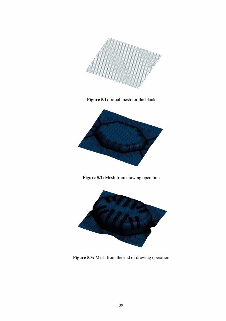
39

Figure 5.1: Initial mesh for the blank

Figure 5.2: Mesh from drawing operation

Figure 5.3: Mesh from the end of drawing operation

40

5.2.3 Punch Speed

Generally, punch velocity is defined about 1mm/sec, which can be considered as

quasi-static speed and as a result of this speed interval, it is not necessary to take the

strain rate sensivity for the materials into consideration.

5.2.4 Blank Holder Force

In this process, blank holder force is taken as 100 tonnes. During the evolution of the

process, different results were obtained for the different blank holder forces. Finally,

100 tonnes of blank holder force was agreed to be used for the process.

5.2.5 Friction Coefficient

Friction is one of the most important parameter in sheet metal forming operations.

Since lubrucation slows down the automation, the goal of all proceses is to obtain the

desired geometry without using lubrication.For metal to metal friction, 0.15 friction

is taken as a friction coefficient.

5.2.6 Drawbeads

Drawbeads effect is considerable on the formability characteristics as explained in

section 3.3. As an important point, the equivalent drawbead force is valuable to

mention. In the simulations drawbeads are not simulated as a geometry until

resonable solutions are figured out. In the final evolution stage, equivalent drawbead

forces replaced by the exact geometries to find out the best geometry which effect

the formability in the desired manner.

5.3 Process for the selected panel

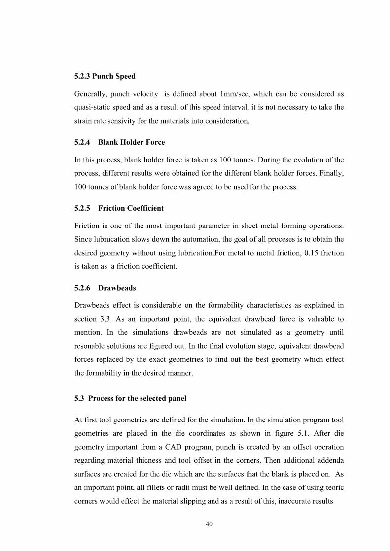
At first tool geometries are defined for the simulation. In the simulation program tool

geometries are placed in the die coordinates as shown in figure 5.1. After die

geometry important from a CAD program, punch is created by an offset operation

regarding material thicness and tool offset in the corners. Then additional addenda

surfaces are created for the die which are the surfaces that the blank is placed on. As

an important point, all fillets or radii must be well defined. In the case of using teoric

corners would effect the material slipping and as a result of this, inaccurate results

41

obtained.Also selection of layer in the the tools and in blank is the most common

mistake made by the engineers. Offset adjustments must be made by taking the

layers in the consideration.

Figure 5.4: Tool geometries

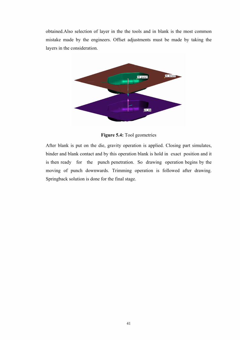
After blank is put on the die, gravity operation is applied. Closing part simulates,

binder and blank contact and by this operation blank is hold in exact position and it

is then ready for the punch penetration. So drawing operation begins by the

moving of punch downwards. Trimming operation is followed after drawing.

Springback solution is done for the final stage.

42

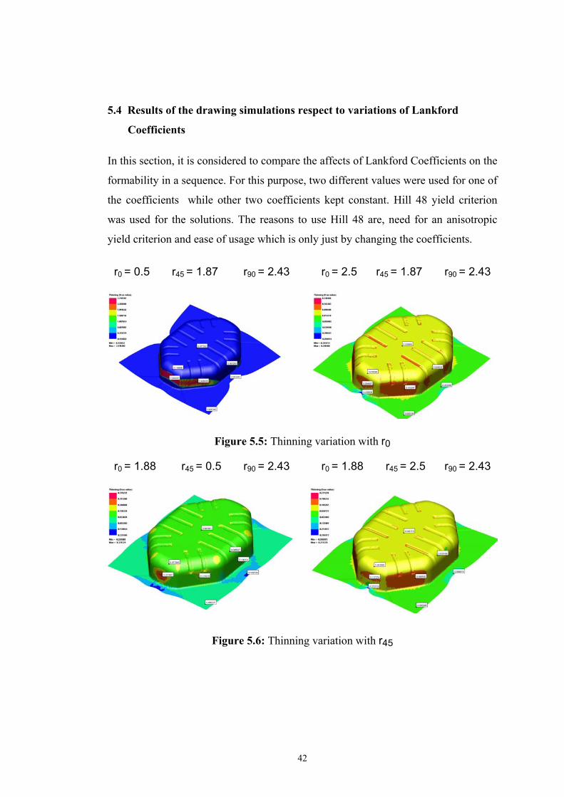
5.4 Results of the drawing simulations respect to variations of Lankford

Coefficients

In this section, it is considered to compare the affects of Lankford Coefficients on the

formability in a sequence. For this purpose, two different values were used for one of

the coefficients while other two coefficients kept constant. Hill 48 yield criterion

was used for the solutions. The reasons to use Hill 48 are, need for an anisotropic

yield criterion and ease of usage which is only just by changing the coefficients.

r0 = 0.5 r45 = 1.87 r90 = 2.43 r0 = 2.5 r45 = 1.87 r90 = 2.43

Figure 5.5: Thinning variation with r0

r0 = 1.88 r45 = 0.5 r90 = 2.43 r0 = 1.88 r45 = 2.5 r90 = 2.43

Figure 5.6: Thinning variation with r45

43

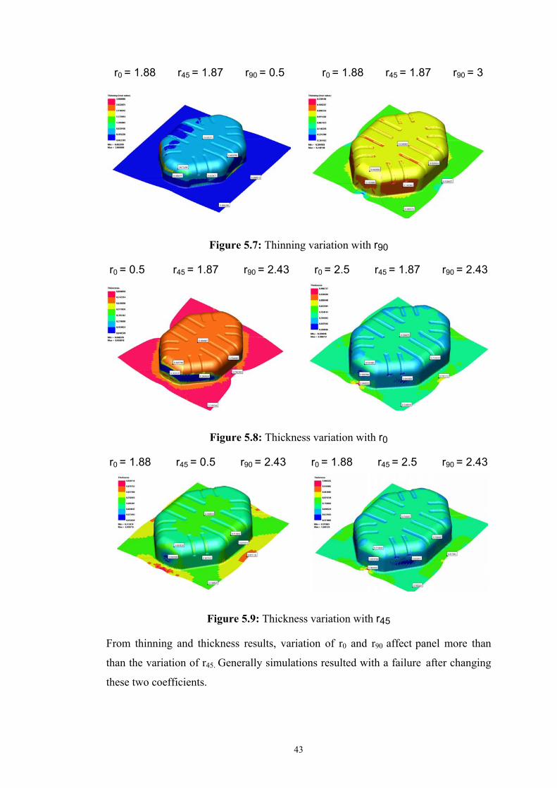
r0 = 1.88 r45 = 1.87 r90 = 0.5 r0 = 1.88 r45 = 1.87 r90 = 3

Figure 5.7: Thinning variation with r90

r0 = 0.5 r45 = 1.87 r90 = 2.43 r0 = 2.5 r45 = 1.87 r90 = 2.43

Figure 5.8: Thickness variation with r0

r0 = 1.88 r45 = 0.5 r90 = 2.43 r0 = 1.88 r45 = 2.5 r90 = 2.43

Figure 5.9: Thickness variation with r45

From thinning and thickness results, variation of r0 and r90 affect panel more than

than the variation of r45. Generally simulations resulted with a failure after changing

these two coefficients.

44

r0 = 1.88 r45 = 1.87 r90 = 0.5 r0 = 1.88 r45 = 1.87 r90 = 3

Figure 5.10: Thickness variation with r90

r0 = 0.5 r45 = 1.87 r90 = 2.43 r0 = 2.5 r45 = 1.87 r90 = 2.43

Figure 5.11: Major strain variation with r0

r0 = 1.88 r45 = 0.5 r90 = 2.43 r0 = 1.88 r45 = 2.5 r90 = 2.43

Figure 5.12: Major strain variation with r45

45

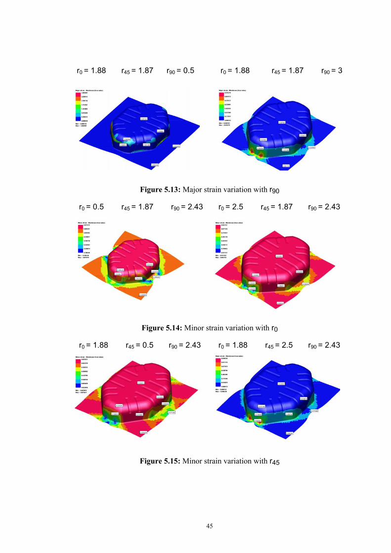
r0 = 1.88 r45 = 1.87 r90 = 0.5 r0 = 1.88 r45 = 1.87 r90 = 3

Figure 5.13: Major strain variation with r90

r0 = 0.5 r45 = 1.87 r90 = 2.43 r0 = 2.5 r45 = 1.87 r90 = 2.43

Figure 5.14: Minor strain variation with r0

r0 = 1.88 r45 = 0.5 r90 = 2.43 r0 = 1.88 r45 = 2.5 r90 = 2.43

Figure 5.15: Minor strain variation with r45

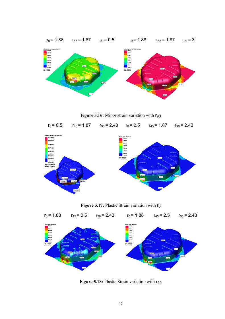
46

r0 = 1.88 r45 = 1.87 r90 = 0.5 r0 = 1.88 r45 = 1.87 r90 = 3

Figure 5.16: Minor strain variation with r90

r0 = 0.5 r45 = 1.87 r90 = 2.43 r0 = 2.5 r45 = 1.87 r90 = 2.43

Figure 5.17: Plastic Strain variation with r0

r0 = 1.88 r45 = 0.5 r90 = 2.43 r0 = 1.88 r45 = 2.5 r90 = 2.43

Figure 5.18: Plastic Strain variation with r45

47

r0 = 1.88 r45 = 1.87 r90 = 0.5 r0 = 1.88 r45 = 1.87 r90 = 3

Figure 5.19: Plastic Strain variation with r90

r0 = 0.5 r45 = 1.87 r90 = 2.43 r0 = 2.5 r45 = 1.87 r90 = 2.43

Figure 5.20: FLD variation with r0

In figure 5.21 below, variation of FLD with r45 is shown. Apperently, r45 seems to

affect the diagram lesser than the other coefficients, but this may not be a

generalization because of the consideration of the interactions of many features that

could influence the results to alter.

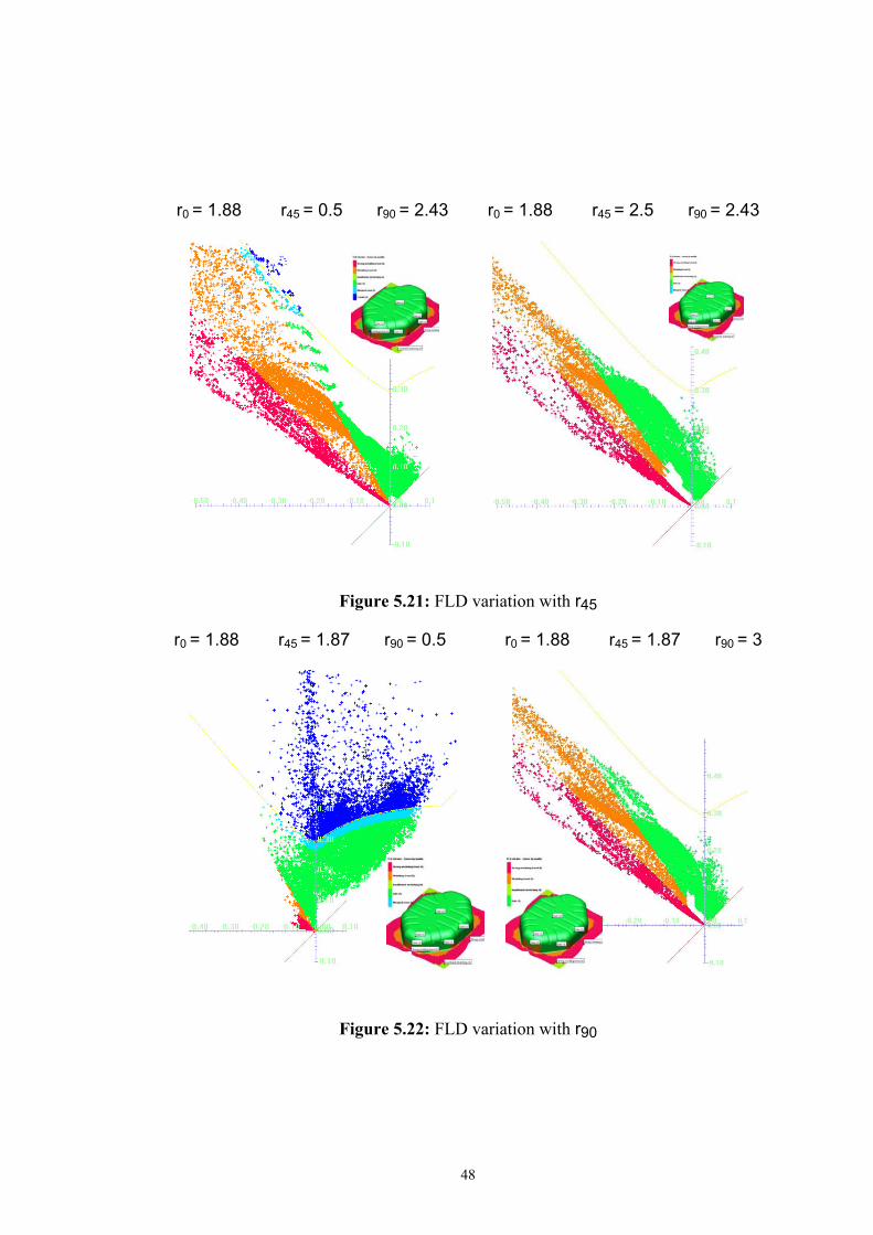
48

r0 = 1.88 r45 = 0.5 r90 = 2.43 r0 = 1.88 r45 = 2.5 r90 = 2.43

Figure 5.21: FLD variation with r45

r0 = 1.88 r45 = 1.87 r90 = 0.5 r0 = 1.88 r45 = 1.87 r90 = 3

Figure 5.22: FLD variation with r90

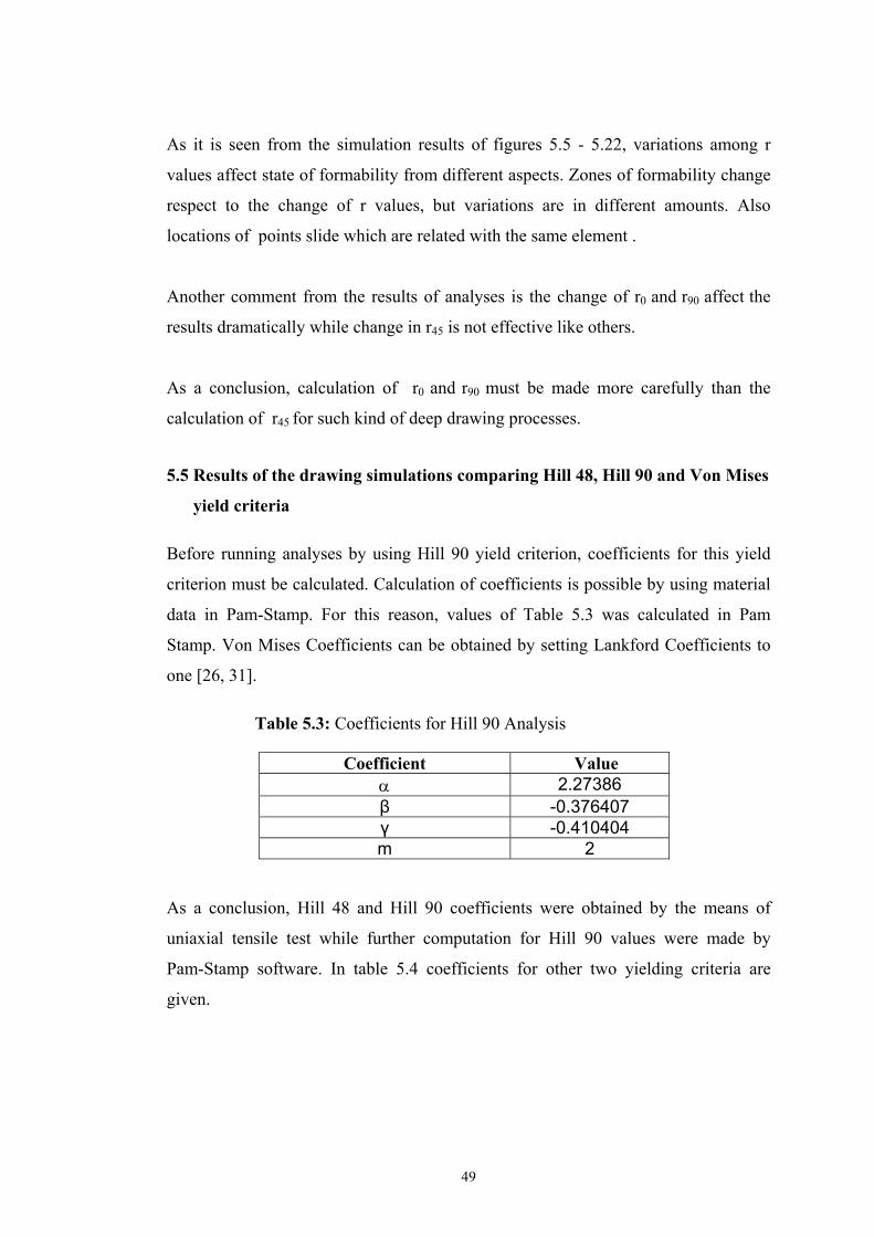
49

As it is seen from the simulation results of figures 5.5 - 5.22, variations among r

values affect state of formability from different aspects. Zones of formability change

respect to the change of r values, but variations are in different amounts. Also

locations of points slide which are related with the same element .

Another comment from the results of analyses is the change of r0 and r90 affect the

results dramatically while change in r45 is not effective like others.

As a conclusion, calculation of r0 and r90 must be made more carefully than the

calculation of r45 for such kind of deep drawing processes.

5.5 Results of the drawing simulations comparing Hill 48, Hill 90 and Von Mises

yield criteria

Before running analyses by using Hill 90 yield criterion, coefficients for this yield

criterion must be calculated. Calculation of coefficients is possible by using material

data in Pam-Stamp. For this reason, values of Table 5.3 was calculated in Pam

Stamp. Von Mises Coefficients can be obtained by setting Lankford Coefficients to

one [26, 31].

Table 5.3: Coefficients for Hill 90 Analysis

Coefficient Value α 2.27386 β -0.376407 γ -0.410404 m 2

As a conclusion, Hill 48 and Hill 90 coefficients were obtained by the means of

uniaxial tensile test while further computation for Hill 90 values were made by

Pam-Stamp software. In table 5.4 coefficients for other two yielding criteria are

given.

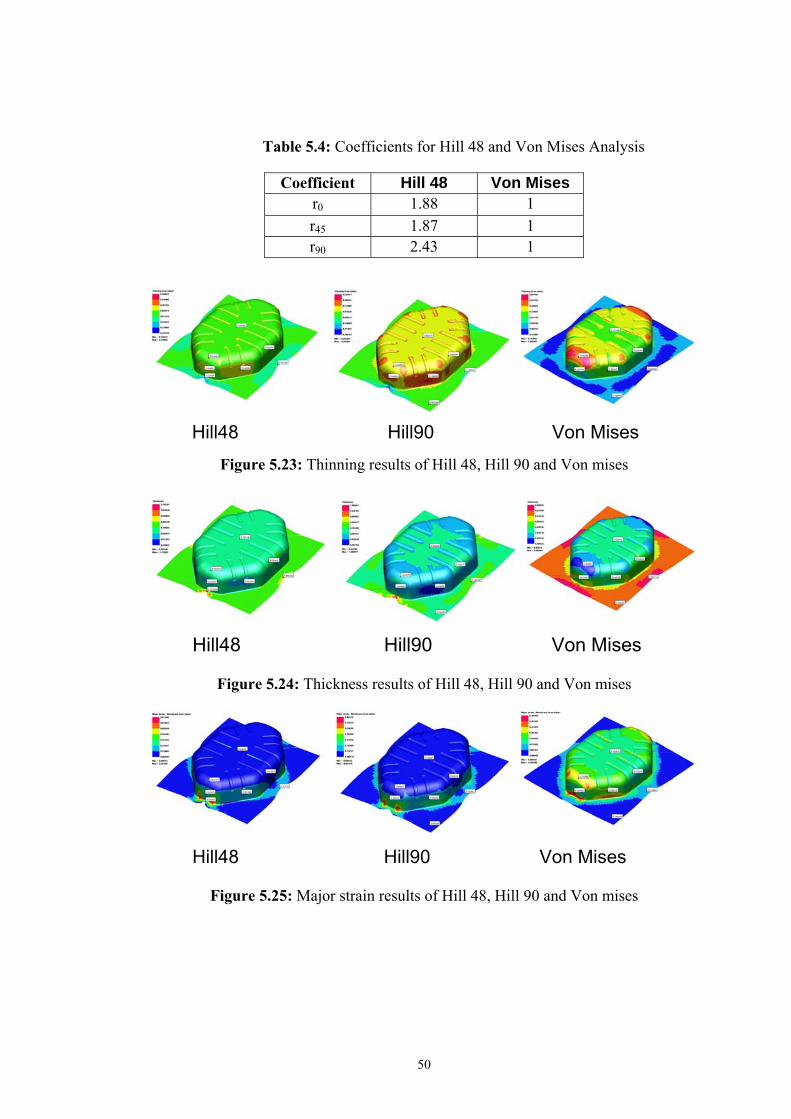
50

Hill48 Hill90 Von Mises

Table 5.4: Coefficients for Hill 48 and Von Mises Analysis

Coefficient Hill 48 Von Mises r0 1.88 1 r45 1.87 1 r90 2.43 1

Figure 5.23: Thinning results of Hill 48, Hill 90 and Von mises

Figure 5.24: Thickness results of Hill 48, Hill 90 and Von mises

Figure 5.25: Major strain results of Hill 48, Hill 90 and Von mises

Hill48 Hill90 Von Mises

Hill48 Hill90 Von Mises

51

Figure 5.26: Minor strain results of Hill 48, Hill 90 and Von mises

Figure 5.27: Plastic strain results of Hill 48, Hill 90 and Von mises

Figure 5.28: Results of formability zones of Hill 48, Hill 90 and Von mises

Hill48 Hill90 Von Mises

Hill48 Hill90 Von Mises

Hill48 Hill90 Von Mises

52

Figure 5.29: FLD results of Hill 48, Hill 90 and Von mises

According to the comparison of the simulation results and mesurements from the

actual panel, Hill 48 is said to give more reliable results than the others. Regarding

thinning and thickness measurements, values of the side wall and flange regions are

so close to the simulation results. From the result of FLD diagram of Hill 48 solution,

cracking regions are obtained which are can be seen in the thinning or thickness

simulations also. Moreover, these results fit to the measurements of the actual panel.

Another important point is the wrinkling results. In Hill 48 simulations, there are

regions that have wrinkling tendency while in Hill 90 simulations there are no

regions that have wrinkling tendency observed.

Although the calculations are not accurate in this work, Hill 90 solutions are

expected to be more accurate than the Hill 48 solutions according to the papers

related to this field . Probable mistake may be the miscalculated coefficients for this

yield criteria.

As it is seen from the results of the Von Mises solution, thinning, thickness and the

shape of the panel of simulations are not even close to the real data. From these

results, one can understand the significance of using anisotropic yield criteria while

working with the sheet metals.

Hill48 Hill90 Von Mises

53

5.6 Results of the contact force and punch penetration comparing Hill 48

Hill 90 and Von Mises yielding criteria

According to the contact force vs. punch penetration results, it is obtained that punch

penetrates about 185 mm. which is also nearly the height of the wheelhouse panel

and at the and of this penetration, punch force yields about 600 kN. In the simulation

applications, BHF is adjusted to obtain the panel without any wrinkles or cracks and

which is later to be added to the punch force to obtain the minimum press tonnage.

In the simulation results non of these three yield criteria make any difference until

the end of the penetration process. The peak after 185 mm is related to the contact of

the punch, die and sheet interaction.

Figure 5.30: Contact force results of Hill 48, Hill 90 and Von Mises

In figure 5.31 strain path forming for different Lankford Coefficients are obtained.

According to this figure, different Lankford Coefficients create different strain paths.

So, it is one of the ways to explain the strain path orientation in FLD diagrams for

the same element with same material under different Lankford Coefficients.

Hill48 Hill90 Von Mises

54

Figure 5.31: Strain paths for different anisotropy coefficients

5.7 Comparison of the results by using normal anisotropy value of 2.01 and

Lankford Coefficients of 1.88, 1.87 and 2.43

As it is mentioned before calculation of the normal anisotropy value can be made

according to the equation (4.2). According to this equation, normal anisotropy value

for the used material is 2.01. This section is separated from 5.8 because the material

data and Lankford Coefficients which are used in this section are taken from the test

results.

Results of analyses of these two cases are below:

Figure 5.32: Thinning results with r values of 1.88, 1.87, 2.43 and R of 2.01

Lankford Coefficients

Normal anisotropy

6:0.5-1.87-2.43 7:2.5-1.87-2.43 8:1.88-0.5-2.43 9:1.88-2.5-2.43 10:1.88-1.87-0.5 11:1.88-1.8-3

55

Figure 5.33: Thickness results with r values of 1.88, 1.87, 2.43 and R of 2.01

Figure 5.34: Major strain results with r values of 1.88, 1.87, 2.43 and R of 2.01

Figure 5.35: Minor strain results with r values of 1.88, 1.87, 2.43 and R of 2.01

Although the values of Lankford Coefficients are not far apart from 2.01, all results

have variations when they are compared. By the way, results of both analyses can

be compared with the actual panel data to figure out which method yield better

results.

Normal anisotropy

Lankford Coefficient

Normal anisotropy

Lankford Coefficient

Normal anisotropy

Lankford Coefficient

56

Figure 5.36: Formability zone results with r values of 1.88, 1.87, 2.43 and R of 2.01

Figure 5.37: FLD results with r values of 1.88, 1.87, 2.43 and R of 2.01

According to the figures 5.32 - 5.37, results of the same points are varying and

results that are obtained with the Lankford coefficients are more reliable than the

results obtained with normal anisotropy value according to the measures of actual

panel. Actual panel fails near flange and side wall curl regions as it seen from the

simulation results that are performed by Lankford coefficients.

5.8 Comparison of the simulation results by using Lankford Coefficients that

have normal anisotropy value of 2.01

The aim of this examination is to show the differences in the results of different

Lankford Coefficients that yield the value of 2.01 as the normal anisotropy

coefficient when put in the equation (4.2). By this application, variations among the

results of Lankford Coefficient’s and normal anisotropy can be figured out.

Additionally, since these coefficients are not as same as the measured coefficients or

Lankford Coefficient

Normal anisotropy

Normal anisotropy

Lankford Coefficient

57

actual material data, results are not compared with the actual panel. On the other

hand, the goal of this section is to find an answer to the question of using normal

anisotropy value in simulations The coefficients subjected to this study can be seen

in the table 5.5 below.

Table 5.5: Lankford Coefficients which were set to obtain normal anisotropy value

of 2.01

Analysis r0 r45 r90 R 1 2.43 1.88 1.87 2.01 2 1.88 2.15 1.87 2.01 3 2.35 1.7 2.3 2.01 4 2.1 1.9 2.15 2.01 5 1.8 2.1 2.05 2.01 6 1 2.28 2.5 2.01 7 2.92 1.1 2.92 2.01 8 2.5 2.28 1 2.01

Figure 5.38: Thinning results with r values of 2.43, 1.88, 1.87 and R value of 2.01

Figure 5.39: Thickness results with r values of 2.43, 1.88, 1.87 and R value of 2.01

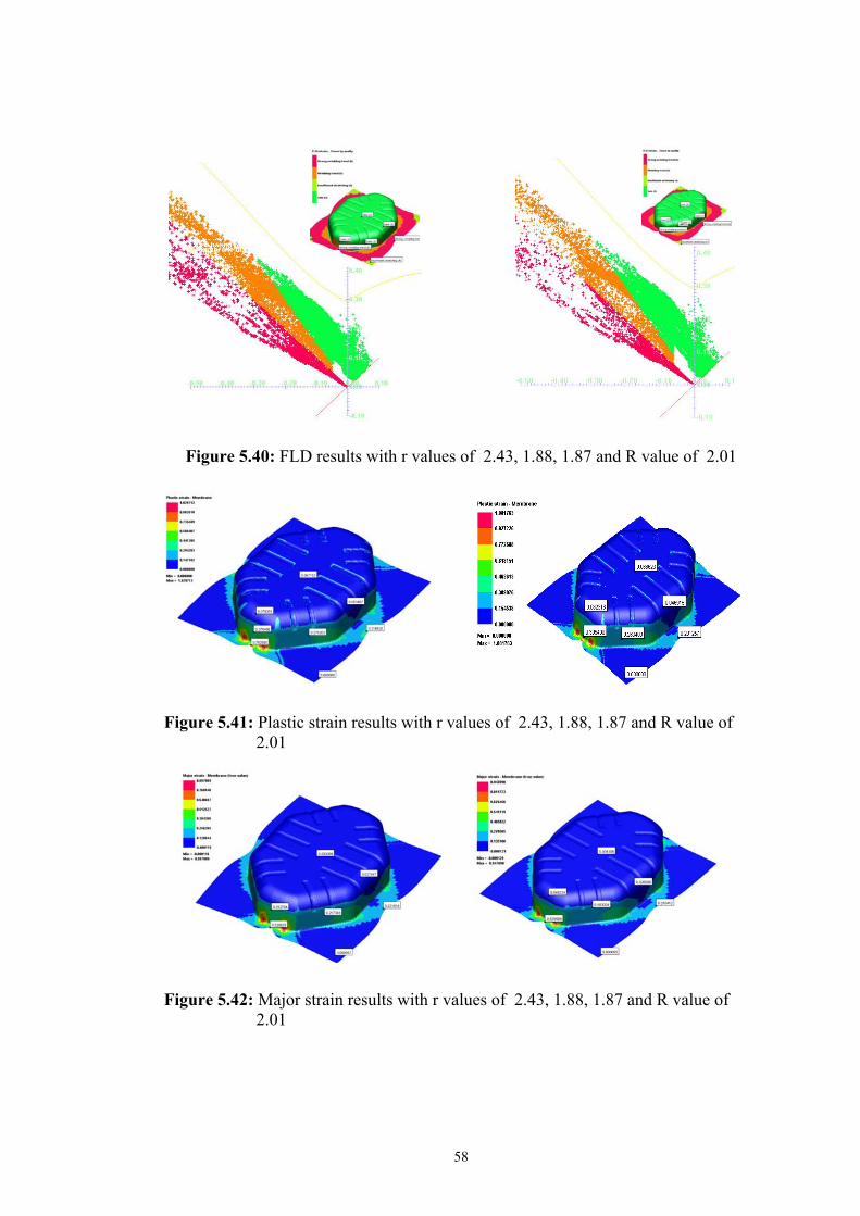
58

Figure 5.40: FLD results with r values of 2.43, 1.88, 1.87 and R value of 2.01

Figure 5.41: Plastic strain results with r values of 2.43, 1.88, 1.87 and R value of 2.01

Figure 5.42: Major strain results with r values of 2.43, 1.88, 1.87 and R value of 2.01

59

Figure 5.43: Minor strain results with r values of 2.43, 1.88, 1.87 and R value of 2.01

As a result for this simulations according to the figures 5.38 - 5.43, results at the

same points are not change significantly. Results of the FLD are not change either.

At a glance, results seem to be very close but one must bear in mind that, the order of

anisotropy values were altered.

Figure 5.44: Thinning results with r values of 1.88, 2.15, 1.87 and R value of 2.01

Figure 5.45: Thickness results with r values of 1.88, 2.15, 1.87 and R value of 2.01

60

Figure 5.46: FLD results with r values of 1.88, 2.15, 1.87 and R value of 2.01

Figure 5.47: Plastic strain results with r values of 1.88, 2.15, 1.87 and R value of 2.01

Figure 5.48: Major strain results with r values of 1.88, 2.15, 1.87 and R value of 2.01

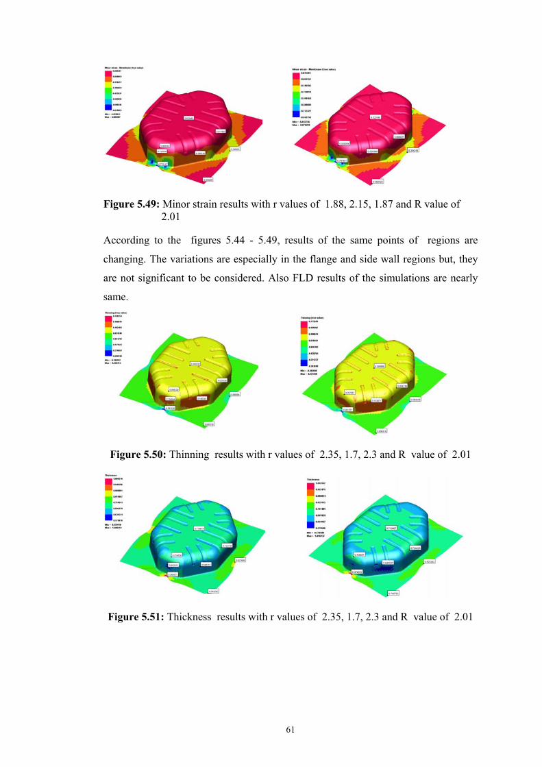
61

Figure 5.49: Minor strain results with r values of 1.88, 2.15, 1.87 and R value of 2.01

According to the figures 5.44 - 5.49, results of the same points of regions are

changing. The variations are especially in the flange and side wall regions but, they

are not significant to be considered. Also FLD results of the simulations are nearly

same.

Figure 5.50: Thinning results with r values of 2.35, 1.7, 2.3 and R value of 2.01

Figure 5.51: Thickness results with r values of 2.35, 1.7, 2.3 and R value of 2.01

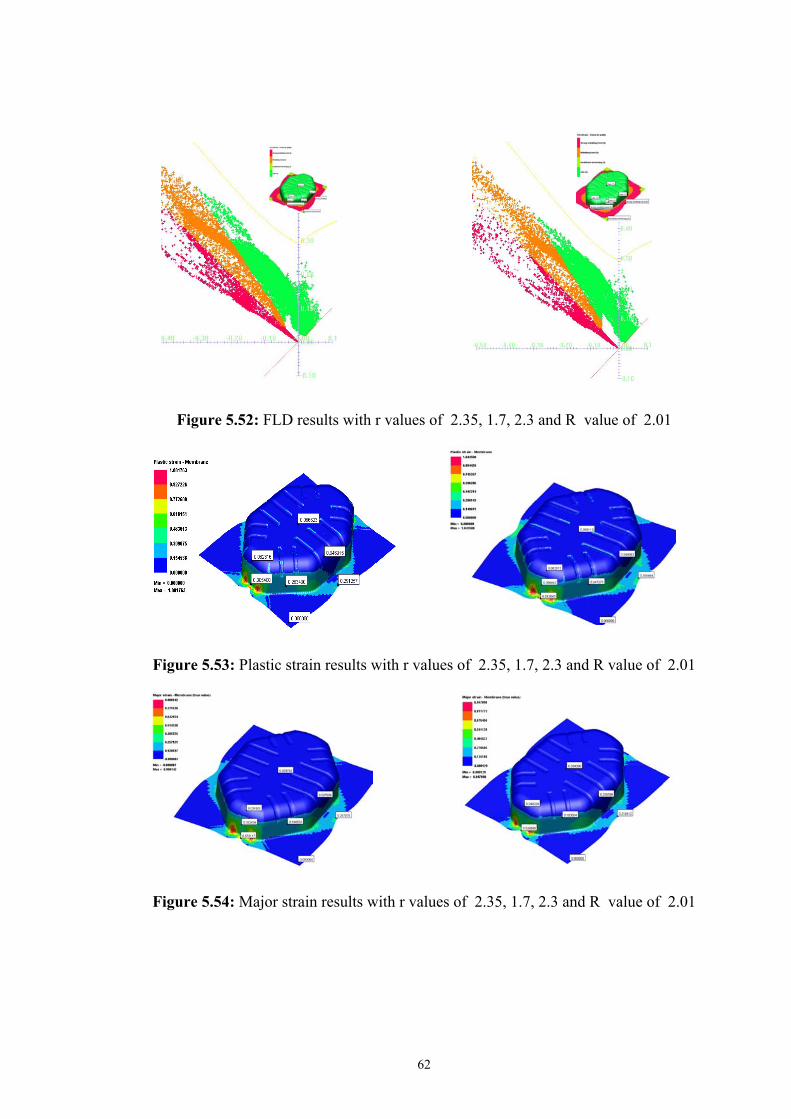
62

Figure 5.52: FLD results with r values of 2.35, 1.7, 2.3 and R value of 2.01

Figure 5.53: Plastic strain results with r values of 2.35, 1.7, 2.3 and R value of 2.01

Figure 5.54: Major strain results with r values of 2.35, 1.7, 2.3 and R value of 2.01

63

Figure 5.55: Minor strain results with r values of 2.35, 1.7, 2.3 and R value of 2.01

According to the figures 5.50- 5.55, results of the same points are not change

significantly. Beside this, FLD is not indicate any major variation.

Figure 5.56: Thinning results with r values of 2.1, 1.9, 2.15 and R value of 2.01

Figure 5.57: Thickness results with r values of 2.1, 1.9, 2.15 and R value of 2.01

64

Figure 5.58: FLD results with r values of 2.1, 1.9, 2.15 and R value of 2.01

Figure 5.59: Plastic strain results with r values of 2.1, 1.9, 2.15 and R value of 2.01

Figure 5.60: Major strain results with r values of 2.1, 1.9, 2.15 and R value of 2.01

65

Figure 5.61: Minor strain results with r values of 2.1, 1.9, 2.15 and R value of 2.01

According to the figures 5.56 - 5.61, results at the same points are close to each

other but, as it is seen, marginal zone result is obtained which could fail the panel

due to different Lankford Coefficients and it is not seen in the normal anisotropy

results.

Figure 5.62: Thinning results with r values of 1.8, 2.1, 2.05 R value of 2.01

Figure 5.63: Thickness results with r values of 1.8, 2.1, 2.05 and R value of 2.01

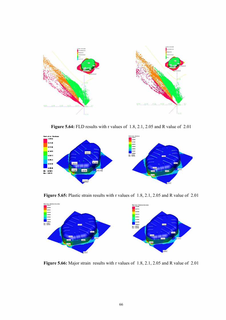
66

Figure 5.64: FLD results with r values of 1.8, 2.1, 2.05 and R value of 2.01

Figure 5.65: Plastic strain results with r values of 1.8, 2.1, 2.05 and R value of 2.01

Figure 5.66: Major strain results with r values of 1.8, 2.1, 2.05 and R value of 2.01

67

Figure 5.67: Minor strain results with r values of 1.8, 2.1, 2.05 and R value of 2.01

According to the figures 5.62- 5.67, some results of the same points are not changed

significantly but, for some points, marginal zone result is obtained which could fail

the panel due to different Lankford Coefficients.

Figure 5.68: Thinning results with r values of 1, 2.28, 2.5 and R value of 2.01

Figure 5.69: Thickness results with r values of 1, 2.28, 2.5 and R value of 2.01

68

Figure 5.70: FLD results with r values of 1, 2.28, 2.5 and R value of 2.01

Figure 5.71: Plastic strain results with r values of 1, 2.28, 2.5 and R value of 2.01

Figure 5.72: Major Strain results with r values of 1, 2.28, 2.5 and R value of 2.01

69

Figure 5.73: Minor strain results with r values of 1, 2.28, 2.5 and R value of 2.01

According to the figures 5.68 - 5.73, overall thinning or thickness are not change

significantly except flange and side wall regions. On the other hand, many points

prone to enter the cracking zone according to the FLD, which is not seen with normal

anisotropy solution. Also, variation of r0 must be taken into consideration for this

results.

Figure 5.74: Thinning results with r values of 2.92, 1.1, 2.92 and R value of 2.01

Figure 5.75: Thickness results with r values of 2.92, 1.1, 2.92 and R value of 2.01

70

Figure 5.76: FLD results with r values of 2.92, 1.1, 2.92 and R value of 2.01

Figure 5.77: Plastic strain results with r values of 2.92, 1.1, 2.92 and R value of 2.01

Figure 5.78: Major strain results with r values of 2.92, 1.1, 2.92 and R value of 2.01

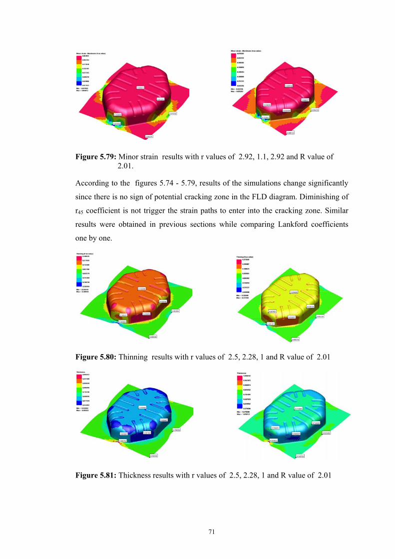
71

Figure 5.79: Minor strain results with r values of 2.92, 1.1, 2.92 and R value of 2.01.

According to the figures 5.74 - 5.79, results of the simulations change significantly

since there is no sign of potential cracking zone in the FLD diagram. Diminishing of

r45 coefficient is not trigger the strain paths to enter into the cracking zone. Similar

results were obtained in previous sections while comparing Lankford coefficients

one by one.

Figure 5.80: Thinning results with r values of 2.5, 2.28, 1 and R value of 2.01

Figure 5.81: Thickness results with r values of 2.5, 2.28, 1 and R value of 2.01

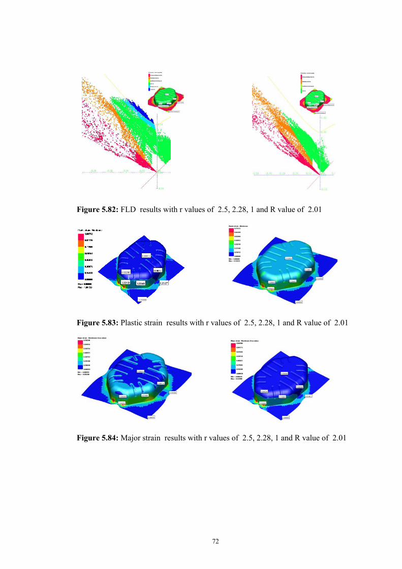
72

Figure 5.82: FLD results with r values of 2.5, 2.28, 1 and R value of 2.01

Figure 5.83: Plastic strain results with r values of 2.5, 2.28, 1 and R value of 2.01

Figure 5.84: Major strain results with r values of 2.5, 2.28, 1 and R value of 2.01

73

Figure 5.85: Minor strain results with r values of 2.5, 2.28, 1 and R value of 2.01

According to the figures 5.80 - 5.85, results of the simulations vary significantly.

Results with the Lankford coefficients are also indicate the sign of a failure. From

this point of view, avability of such kind of distribution for Lankford Coefficients

must be considered.

74

6. CONCLUSIONS AND RECOMMENDATIONS

As it is well known, desired final shape of the parts is leaded by the material

behaviour. From this view, characterization of material behaviours under several

deformation modes such as uniaxial tension, pure shear, uniaxial compression, plane

strain etc. is very significant for the development of the process. Before using the

materials, related test must be made to figure out the limits of the material.

By using computers, process for desired geometry simulated by calculation of

equations which are strain hardening, yielding criteria and hardening type. For this

reason, measurements for material characterization and selections for deriving

equations are significant for accurate results.

The results of simulations nearly observed in the actual data. Locations of tearing

and the regions prone to wrinkling are observed and precautions were made to obtain

the desired final shape.

As it is obtained from simulations, results with Lankford Coefficients and normal

anisotropy value which is obtained from the same Lankford Coefficients yield

different results if value of one of these coefficients is not close to others. On the

other hand, availability of such kind of condition might be subjected to another

survey.

In this thesis, results for kinematic hardening which is known for its better accuracy

could not be obtained, because of the coefficient data for the yielding criteria using

kinematic hardening rules was not available. Additionally, results obtained by using

kinematic hardening give more accurate results especially for springback problems

regarding to the papers related to this field. So, the ways of using this hardening

models must be searched for further development.

75

REFERENCES

[1] Marciniak, Z., Duncan, J.L., and Hu, S.J., 2002. Mechanics of sheet metal forming, Butterworth-Heinemann.

[2] Arwidson, C., 2005. Numerical Simulation of Sheet Metal Forming for High

Strength Steels, Licentiate Thesis, Lulea University of Technology, Sweden, ISSN 1402-1757.

[3] Hu, W., He, J., Anisotropic Behaviors and Its Application on Sheet Metal

Stamping Proceses, ETA-Engineering Technology Associates, Inc. [4] Gau, J.T., 1999.A Study of the Influence of the Bauschinger Effect on

Springback In Two-Dimensional Sheet Metal Forming, Ph.D. Thesis, School of The Ohio State University, USA.

[5] Schuler GmbH., 1998. Metal Forming Handbook , Göppingen, Germany, ISBN

3-540-61185-1. [6] Butuc, M.C.,Gracio, Barata da Rocha, J.J., A., 2002. A theoretical Study on

Forming Limit Diagrams Prediction, Journal of Material Processing Technology, 714-724

[7] Hill, R., 1950. The Mathematical Theory of Plasticity, Oxford University Press,

New York,USA. [8] Xu, S., Weinmann, K.J., 1999. Comparison of Hill’s Yield Criteria in Forming

Limit Predictions, SAE Technical Paper Series, 1999-01-0999. [9] Friedman, P.A., Pan, J. 1998. Effects of plastic Anisotropy and Yield Criteria

on Prediction of Forming Limit Curves, International Journal of Mechanic Sciences 42 (2000) 29-48

[10] Önder, İ.E., 2005. Assesment of Sheet Metal Forming Processes by Numerical

Experiments, MSC. Thesis, METU [11] Çiçek, O., 2005. Effects of Drawbeads in Sheet Metal Forming, MSC. Thesis,

ITU [12] Hu, W., Liu, S.-D., 2002. Enhancement of Yield Criteria Considering

Anisotropic Behaviors of Sheet Metals, SAE Technical Paper Series, 2002-01-0158, ISSN 0148-7191

[13] Johnson, W., Mellor, P.B., 1983. Engineering Plasiticity, Ellis Horwood

Limited, Chichester, England.

76

[14] Altan, T., 2004, Short Course on Sheet Metal Forming, Material Properties and Formability, The Ohio State University, Columbus, Ohio.

[15] Altan, T., 2004, Short Course on Sheet Metal Forming, Friction and lubrication in Sheet Metal Forming, The Ohio State University, Columbus, Ohio.

[16] Altan, T., 2004, Short Course on Sheet Metal Forming, Bending, The Ohio

State University, Columbus, Ohio. [17] Altan, T., 2004, Short Course on Sheet Metal Forming, Flanging and Hemming,

The Ohio State University, Columbus, Ohio. [18] Altan, T., 2004, Short Course on Sheet Metal Forming, Deep Drawing of

Round Cups, The Ohio State University, Columbus, Ohio. [19] Altan, T., 2004, Short Course on Sheet Metal Forming, Bending, The Ohio

State University, Columbus, Ohio. [20] Altan, T., 2004, Short Course on Sheet Metal Forming, Introduction to Sheet

Metal Forming Process, The Ohio State University, Columbus, Ohio. [21] Geng, L., Wagoner, R.H., 2002. Role of Plastic Anisotropyt and ıts Evolution

on Springback, International Journal of Mechanical Science 44(2002) 123 – 148.

[22] Sadagopan, S., Urban, D., 2003, Formability Characterization of a new

generation of high strength steels,AISI/DOE Technology Roadmap Program Final Report, Pittsburg

[23] Lumin G., 2000. Application of Plastic Anisotropy and Non-Isotropic Hadening

To Springback Prediction, Ph.D. Thesis, The Ohio State University, Columbus, Ohio.

[24] Kim, J.-B.,Yang,D.-Y.,Yoon J.-W.,Barlat, F., 2000. The Effect of Plastic

Anisotropy on Compressive Instability in Sheet Metal Forming, International Journal of Plasticity, 16(2000) 649-676

[25] Worswick, M.J., Finn, M.J., 2000. The Numerical Simulation of Stretch

Flange Forming, International Journal of Plasticity, 16(2000) 701-720 [26] Pam Stamp 2G, Version 2004.1, 2005. PAMSTAMP-2G User’s Guide, Parc

Club du Golf 13856 Aix en Provence cedex 3 France. [27] Vial-Edwards, C., 1997. Yield Loci of FCC and BCC Sheet Metals,

International Journal of Plasticity, Vol. 13, No. 5, pp.521-531. [28] Green, D.E.,Black, K.C., 2002. A Visual Technique to Determine the Forming

Limit for Sheet Materials, SAE Technical Paper Series, 2002-01-1062.

77

[29] Issa, J., 2004. Forming Limit Diagrams, MSc. Thesis, Michigan State University.

[30] Uk Youn, C., 1993. Plane Strain Finite Element Analysis of Sheet Forming

operations Including Bending Effects, Ph.D. Thesis, The Ohio State University, Columbus, Ohio.

[31] Pam Stamp 2G, Version 2004.1, 2005. PAMSTAMP-2G Reference Manual,

Parc Club du Golf 13856 Aix en Provence cedex 3 France. [32] Wang, C., 1993. Mechanics of Bending, Flanging, and Deep Drawing and a

Computer-Aided Modeling System for Predictions of Strain, Fracture, Wrinkling and Springback in Sheet Metal Forming, Ph.D. Thesis, The Ohio State University, Columbus, Ohio.

78

BIBLIOGRAPHY

Göktuğ ÇINAR was born in Tekirdağ at 1977. He enrolled Mechanical Engineering Department at Istanbul Technical University in 1997. He was graduated from this department in 2002. His master education at Solid Mechanics Program of the Mechanical Engineering Department in ITU is going on and he also works as process and quality engineer at Tool & Die and Prototype Manufacturing Department in Ford-Otosan.