effects analysis for the delta smelt fall habitat …...water project (swp) and central valley...

EFFECTS ANALYSIS FOR THE DELTA SMELT FALL HABITAT ACTION IN 2019

S U B M I T T E D BY:

United States Bureau of Reclamation

August 2019

Effects Analysis for the Delta Smelt Fall Habitat Action in 2019 August, 2019 ii

Contents

Tables ........................................................................................................................................................... iii

Figures ......................................................................................................................................................... iv

Introduction .................................................................................................................................................. 1

Project Description ....................................................................................................................................... 4 Habitat Studies and Actions ................................................................................................ 4

Status of Delta Smelt .................................................................................................................................... 7 Long-Term Delta Smelt Abundance Trends ........................................................................ 7 Current Delta Smelt Spatial Distribution .......................................................................... 10

Effects Analysis ........................................................................................................................................... 13 Introduction to the Effects Analysis ................................................................................. 13 Existing Conditions through July 30th, 2019 ..................................................................... 13 Forecasted 2019 Fall X2 Operations ................................................................................. 17 Effects on Delta Smelt ....................................................................................................... 21

Application to the 2019 Proposed Action ............................................................................................. 26

Effects on Delta Smelt Critical Habitat ............................................................................. 29 Salinity, Abiotic Habitat Index, and Hydrodynamics-Based Station Index ............................................ 30

Food Availability in the Low Salinity Zone ............................................................................................. 69

Entrainment Effects .......................................................................................................... 69

Conclusions .................................................................................................... Error! Bookmark not defined.

References .................................................................................................................................................. 72

Effects Analysis for the Delta Smelt Fall Habitat Action in 2019 August, 2019 iii

Tables Table 1. Forecasted Monthly Mean X2 (km) from Mean Daily, August-November, 2019. ........................ 18

Table 2. Forecasted End of Month Storage (TAF), September-December, 2019. ...................................... 19

Table 3. Forecasted Delta outflow and SWP and CVP Exports (cfs), September-December, 2019. ........... 19

Table 4. Model selection for the effect of fall Stock (FMWT index) and X2 fit to juvenile recruitment (log(R/S)) using 1987–2004 data (n = 17). ....................................................................................... 25

Table 5. Model selection for the effect of fall Stock (FMWT index) and X2 fit to juvenile recruitment (log(R/S)) using 1987–2018 data (n = 31). ....................................................................................... 26

Table 6. Average Hydrodynamics-Based Station Index (SIH) In Relation to X2. ......................................... 67

Table 7. Percentiles of Mean X2 in Wet Years, 1960-2015/2016 ............................................................... 69

Effects Analysis for the Delta Smelt Fall Habitat Action in 2019 August, 2019 iv

Figures

Figure 1. Conceptual Model of Drivers Affecting the Transition from Delta Smelt Juveniles to Subadults. .......................................................................................................................................... 5

Figure 2. Conceptual Model of Drivers Affecting the Transition from Delta Smelt Subadults to Adults. ............................................................................................................................................... 6

Figure 3. IEP Newsletter, November 2018 [Fig. 7]. Annual abundance indices of Delta Smelt from: A) 20 mm Survey (larvae and Juveniles; 1995-2017); B) Summer Townet Survey (juveniles; 1959-2017); C) Fall Midwater Trawl Survey (sub-adults; 1967-2017). Inset graphics show most recent 5 years in more detail .................................................................................................. 9

Figure 4. July Results for EDSM. FWS, July 26, 2019. .................................................................................... 10

Figure 5. EDSM Results for July 2019. Source: FWS EDSM Report, July 26, 2019. ....................................... 12

Figure 6a. Observed mean daily EC in western Delta for 2019 compared to 2011, 2017 and 2018. ..... Error! Bookmark not defined.

Figure 6b. Observed daily water temperature in western Delta for 2019 compared to 2017 and 2018. ..................................................................................................................................................... 36

Figure 7. Mean Daily X2 Forecast, August 1-November 30, 2019. ............................................................... 18

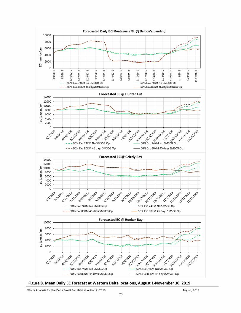
Figure 8. Mean Daily EC Forecast at Western Delta locations, August 1-November 30, 2019 .................... 20

Figure 9. The selected juvenile recruitment model fit to the fall midwater trawl index (a) and mean location of X2 in the months from September to December. ........................................................ 24

Figure 10. Regression coefficients for the five models fit to the original data used in Feyrer et al. 2007 (1987–2004) and updated data (1987–2018). ....................................................................... 25

Figure 11. Posterior Density Distributions from 10,000 Simulations of the Change in Delta Smelt Fall to Summer Recruitment when Mean September-October X2 is Moved from 80 km to 74 km. ................................................................................................................................................... 27

Figure 12. Posterior density distributions from 10,000 simulations of the change in fall to spring recruitment when fall X2 is moved from an upstream location to a downstream location. X2 is measured in river kilometers from the Golden Gate. 81 and 74 kilometers ......................... 28

Figure 13. X2 versus the low salinity (0.5 1– 6 psu) area from Brown et. al. 2014 based on UnTRIM modeling indicates the low salinity area corresponding to 80 km X2 of just over 16000 acres. In 2018, the SMSCG action resulted in over 16000 acres of low salinity area even though the X2 was at ~83.2 km in August and ~84.5 km in September, based on the UnTRIM modeling. .......................................................................................................................... 30

Figure 14. Locations of the Fall Midwater Trawl Sampling Stations included in the Hydrodynamics- Based Station Index Analysis ........................................................................................................... 33

Figure 15. The Percentage of Time With Salinity < 6 psu for X2 = 74 km, As Used in the Hydrodynamics- Based Station Index Analysis. .............................................................................. 34


Figure 17. The Percentage of Time With Salinity < 6 psu for X2 = 76 km, As Used in the

Effects Analysis for the Delta Smelt Fall Habitat Action in 2019 August, 2019 v

Hydrodynamics- Based Station Index Analysis. .............................................................................. 35






Figure 23. Daily average relationship between historically-observed X2 (2.64 mS/cm Surface Conductivity) and 6 psu (10 mS/cm) surface salinity isohaline position. This relationship is measured along the Sacramento River reach for Water Years 1968 – 2012. This figure shows a best-fit regression line, a 95% confidence interval, and the Eq. 1 relationship from Hutton et al. (2015). ........................................................................................................................ 52

Figure 24. The Maximum Depth-Averaged Current Speed, As Used in the Hydrodynamics-Based Station Index Analysis. .................................................................................................................... 54

Figure 25. Average Secchi Depth Versus Monthly-Average X2 for September-December, 2000-2015 (Dashed Lines Show 0.37 m and 0.63 m). ....................................................................................... 55

Figure 26. A) Distribution of Secchi Depth for September 2011; and B) Distribution of Secchi depth Above (Red) and Below (Blue) 0.5 m for September 2011. ............................................................ 57

Figure 27. A) Distribution of Secchi Depth for November 2004; and B) Distribution of Secchi depth Above (Red) and Below (Blue) 0.5 m for November 2004. ............................................................. 58

Figure 28. Hydrodynamics-Based Station Index (SIH) for X2 = 74 km and Low Turbidity. ........................... 60








Figure 36. Hydrodynamics-Based Station Index (SIH) for X2 = 74 km and High Turbidity. ........................... 63






Effects Analysis for the Delta Smelt Fall Habitat Action in 2019 August, 2019 vi



Effects Analysis for the Delta Smelt Fall Habitat Action in 2019 August, 2019 vii

This page left intentionally blank

Effects Analysis for the Delta Smelt Fall Habitat Action in 2019 August, 2019 1

Fall X2 Adaptive Management Plan Proposal

Introduction

The Fall X21 component of the Reasonable and Prudent Alternative (RPA) Action 4 of the US Fish and Wildlife Service’s (USFWS) 2008 Biological Opinion (BiOp) on the coordinated operations of the State Water Project (SWP) and Central Valley Project (CVP) was developed as an adaptive management action, to be tested and refined over the first 10 years of BiOp implementation, based on studies to be conducted during that same period and in consideration of the results of those studies, other new data, other species needs, and other obligations.

At page 369, the BiOp describes the Fall X2 action as follows:

• Objective: Improve fall habitat for Delta Smelt by managing of X2 through increasing Delta

outflow during fall when the preceding water year was wetter than normal. This will help return ecological conditions of the estuary to that which occurred in the late 1990s when smelt populations were much larger. Flows provided by this action are expected to provide direct and indirect benefits to Delta Smelt. Both the direct and indirect benefits to Delta Smelt are considered equally important to minimize adverse effects.

• Action: Subject to adaptive management as described below, provide sufficient Delta outflow

to maintain average X2 for September and October no greater (more eastward) than 74 km in the fall following wet years and 81 km in the fall following above normal years. The monthly average X2 must be maintained at or seaward of these values for each individual month and not averaged over the two-month period. In November, the inflow to CVP/SWP reservoirs in the Sacramento Basin will be added to reservoir releases to provide an added increment of Delta inflow and to augment Delta outflow up to the fall target. The action will be evaluated and may be modified or terminated as determined by the Service.

The BiOp further states at p. 370 that, “…there is a high degree of uncertainty about the quantitative relationship between the size of the Action described above and the expected increment in Delta Smelt recruitment or production.” For this reason, the BiOp requires an Adaptive Management Plan that requires the testing of the conceptual model to elucidate the operative mechanisms and manage accordingly. The BiOp states at p. 283 that:

In accordance with the adaptive management plan, the Service will review new scientific information when provided and may make changes to the action when the best available

1 The distance upstream of the Golden Gate Bridge where the near-bottom, 2-parts-per-thousand isohaline is located.


scientific information warrants…This action may be modified by the Service consistent with the intention of this action based on information provided by the adaptive management program in consideration of the needs of other listed species. Other CVP/SWP obligations may also be considered.

These uncertainties about the efficacy of the action are to be addressed through the adaptive management program, under the Supervision of the Fish and Wildlife Service (BiOp, p. 369).

This 2019 proposal is part of Reclamation and DWR’s implementation of the Fall X2 adaptive management program. It is consistent with the BiOp and ongoing discussions in the Collaborative Science and Adaptive Management Program (CSAMP). The proposed implementation of the Fall X2 action for 2019 considers the hypotheses, analysis, and framework presented in the 2008 BiOp; hydrology occurring in 2019; the need to monitor abiotic and biotic habitat conditions for Delta Smelt; and the needs of other species, including Winter-Run Chinook Salmon on the Sacramento River and Fall-Run Chinook Salmon on the Feather River. The Proposed Action builds upon the 2011 Fall Low Salinity Habitat Studies and Adaptive Management investigations (“FLaSH”), the work of the Collaborative Science and Adaptive Management Program (CSAMP); the adaptive management action in 2017; the synthesis of 2017 results contained in the 2019 Flow Alteration- Management, Analysis and Synthesis team (“FLOAT-MAST”); and the synthesis of results reported in Reclamation’s 2019 Directed Outflow Project (“DOP”).

In 2011, the Fall X2 RPA action was implemented2 at approximately the wet year X2 target of 74 km for September and October. In conjunction with the RPA implementation, a large-scale investigation known as the FLaSH study was implemented by the U.S. Bureau of Reclamation (Reclamation) in cooperation with the Interagency Ecological Program (IEP) to examine hypotheses about the ecological role of low-salinity habitat to support Delta Smelt. Hypotheses about how Delta Smelt and their habitat would respond to increased outflows in the fall were initially presented in the USFWS (2008) BiOp but were developed in more detail through Reclamation’s Fall X2 Adaptive Management Program (AMP). The purpose of the AMP was to provide a focused, science-based evaluation of the Fall X2 RPA for USFWS to consider in their assessment of the effectiveness Fall X2 RPA to support Delta Smelt abundance and habitat. Using a new conceptual model 3 about how Fall X2 may affect Delta Smelt habitat, growth, abundance, and survival, the AMP developed predictions for expected biotic and abiotic habitat responses to X2.

Along with directed FLaSH studies in 2011, the IEP FLaSH synthesis team conducted a comparative analysis of data collected with another wet year (2006) and 2 dry years (2005, 2010) to determine how abiotic and biotic predictions responded in the low salinity zone as function of X2 (Brown et al. 2014). Ultimately, the 2011 FLaSH studies were considered largely inconclusive because many of the key predictions either could not be evaluated with the available data (e.g., primary production), or the necessary data were not collected (e.g., fecundity estimates). Abiotic habitat did increase in 2011 as predicted from the AMP, but other variables such as zooplankton abundance were too variable to

2 In 2011, there was an injunction issued by a federal court in regard to full implementation of the Fall X2 RPA, however the action was mostly met, incidentally, through water releases to meet storage capacity requirements. 3 Conceptual models were developed by the Habitat Study Group (HSG) and FLaSH Synthesis team.


draw a conclusion, and Delta Smelt growth rate comparisons remain incomplete as of 2019. In 2017, a Fall X2 adaptive management action was implemented. The results of the 2017 monitoring program were evaluated in the IEP’s 2019 draft FLOAT-MAST, which concluded that summer water temperatures were a major factor in the condition of Delta Smelt in 2017, stating at p.102:

Given the long periods in July and August >22C we are confident that water temperature had a major negative effect on Delta Smelt in 2017 and is likely a primary factor in the lack of response of the Delta Smelt population to the high flows.

And at p. 104:

Dynamic biotic components were somewhat better in 2017; however, the lack of response of the Delta Smelt population suggests that any benefits of changes in the habitat were minimal.

Reclamation’s draft synthesis of results of the 2017 habitat action are consistent with the draft results from the FLOAT-MAST, finding at p. 342 that:

Preliminary evidence suggests that water temperature, especially in the landward regions of the study area, approached or passed levels (>22-23 C) where physiological stress has been shown to occur (Komoroske et al. 2015) and was primarily responsible for the mortality.

Reclamation and DWR cannot control Delta water temperatures, which are primarily influenced by air temperatures (Kimmerer 2004). However, Reclamation and DWR can provide low salinity habitat in different areas within the fall range of Delta Smelt to provide overlapping components of species habitat within the same region, which is consistent with the conceptual model articulated in Bever et al. (2016). Water year 2019 has provided flows that are similar to 2017 in magnitude and timing. This year is expected to have a different temperatures regime as compared to 2017, which would provide an opportunity to test how species outcomes vary under different temperature regimes in low salinity conditions. Conclusions drawn here about how the proposed 2019 Fall X2 action may affect abiotic and biotic responses follow the basic framework from the FLaSH report and are consistent with the 2008 BiOp. Where the support for predicted responses is considered, the magnitude of effect is then estimated where possible. The effects analysis presented herein follows analyses from the completed FLaSH report (Brown et al. 2014), the FLOAT-MAST and the DOP, along with consideration of additional relevant information for the proposed 2019 Fall X2 action.


Project Description

Refer to the Environmental Assessment for a description on the Proposed Action for fall 2019.

Habitat Studies and Actions

The FLaSH conceptual model suggests that Delta Smelt habitat should include salinity conditions ranging from fresh to low salinity (0-6 psu), minimum turbidity of approximately 12 Nephelometric Turbidity Units (NTU) for adults, temperatures below 25°C, food availability, and bathymetric complexity (FLaSH, pp. 15-23; Komoroske et al. 2015). The goal of the 2019 Proposed Action is to provide low salinity conditions in regions that overlap existing areas of bathymetric complexity. During September and October, the Proposed Action would provide low salinity habitat in the lower Sacramento River, Suisun Bay, and Suisun Marsh into Honker Bay and portions of Grizzly Bay. Biological and habitat monitoring will occur to inform adaptive management. Specifically, Reclamation seeks to enhance ongoing fisheries monitoring programs including the CDFW Summer Townet survey, USFWS EDSM Kodiak Trawl, and UC Davis Suisun Marsh otter trawl survey. The goal of implementing these monitoring programs is to increase the temporal and spatial resolution of the fisheries data they generate.

In addition to the Proposed Action for Fall 2019, a number of habitat actions will be either implemented in 2019 or studied for their potential to be implemented in 2020 or 2021. The overarching driver for these other proposed actions are first, the need to provide greater food availability to Delta Smelt, and second, the need for a greater extent of low salinity zone habitat in areas outside of the main range. Food availability and quality figure prominently in the IEP MAST (2015) conceptual models for the probability of survival from juveniles to subadults in summer (Figure 1) and subadults to adults in the fall (Figure 2). The subadult to adult model also considers the size and location of the low salinity zone to be of importance.


Source: IEP MAST (2015: Figure 48).

Figure 1. Conceptual Model of Drivers Affecting the Transition from Delta Smelt Juveniles to Subadults.


Source: IEP MAST (2015: Figure 49).

Figure 2. Conceptual Model of Drivers Affecting the Transition from Delta Smelt Subadults to Adults.

There have been several food augmentation actions in recent years that appear to have provided species benefits. For example, in 2016 and 2018, DWR implemented the North Delta Flow Action. The general approach is that flow from agricultural drainage or Sacramento River diversions is redirected through the Yolo Bypass Toe Drain as a “pulse flow” to increase food web productivity and transport food downstream to the Cache Slough Complex and lower Sacramento River near Rio Vista. The 2016 action relied on supplemental flows from the Sacramento River, while the 2018 action relied on agricultural return flows. Overall, the results have been variable, with the 2016 action providing downstream transport of food resources while the 2018 results showed less benefit. It is possible that the differences in source water influenced the results. The North Delta Flow Action will be repeated in late August through September 2019, overlapping with the fall habitat adaptive management action (DWR Work Plan 2019). In 2018, the Bureau of Reclamation implemented its Sacramento Deepwater Ship Channel Nutrient Enrichment Project to determine if the addition of nitrogen can stimulate plankton production in a section of the ship channel to benefit Delta Smelt. Initial results were promising and the action was repeated in summer 2019. In addition, monitoring will be undertaken in fall 2019 to test the support


for the conceptual models linking Delta Smelt growth and survival to food availability and the low salinity zone.

Status of Delta Smelt

Long-Term Delta Smelt Abundance Trends

Available survey indices of abundance suggested the current status of Delta Smelt to be poor compared to historic status. The 20-mm Delta Smelt index for 2017 was 1.5, the highest on record since 2013. The 2017 index was calculated from surveys 3-6, during which time 79 Delta Smelt were collected from index stations. Over the course of the 2017 20-mm surveys, a total of 184 Delta Smelt were collected. In 2018, the 20-mm survey index was incalculable due to low catch. In 2019, Delta Smelt were caught in the 20-mm survey but the index value is not yet available. The STN Delta Smelt index for 2017 was 0.2. It is the third-lowest index on record and follows two years in which the index was zero. The FMWT Delta Smelt index for 2017 was 2. In 2017, two Delta Smelt were collected at index stations in October. In 2018, the FMWT abundance index was zero. The 2019 Spring Kodiak Trawl (SKT) Delta Smelt Index of relative abundance was 0.4 and the lowest index on record. The Spring Kodiak Trawl index calculated using 39 stations, each sampled monthly January – April (156 sampling events). Only two Delta Smelt were caught during these sampling events; one was collected in the Sacramento River in January, and one was collected in the Suisun Bay in February. This low index and associated catch was consistent with record low Delta Smelt relative abundance in proceeding 2018 surveys (Figure 3). The Enhanced Delta Smelt Monitoring (EDSM) is a year-round monitoring program focused on sampling Delta Smelt at all life stages. The sampling efforts for EDSM are focusing on six geographic areas where Delta Smelt are likely to be caught based on historic data. The estimated abundance for the week July 1-5, 2019, based on the EDSM by region is as follows: Suisun Bay=5,600, Suisun Marsh=3,030, DWSC=55,963. The estimated abundance for the week of July 22-25, 2019 based on the EDSM by region is as follows: lower Sacramento=1,422, and DWSC=9,638. The total estimated abundance for the end of July is 11,059, with an estimated range of 2,475 to 32,202 (Figure 4). (FWS, July 26, 2019.)


Figure 3. IEP Newsletter, November 2018 [Fig. 7]. Annual abundance indices of Delta Smelt from: A) 20 mm Survey (larvae and Juveniles; 1995-2017); B) Summer Townet Survey (juveniles; 1959-2017); C) Fall Midwater Trawl Survey (sub-adults; 1967-2017). Inset graphics show most recent 5 years in more detail.


Figure 4. July Results for EDSM. FWS, July 26, 2019.

Current Delta Smelt Spatial Distribution

EDSM monitoring data for July 2019 suggest that a substantial portion of the population is in the Deepwater Ship Channel. In July, Delta Smelt have also been caught in the lower Sacramento River, Suisun Bay and Suisun Marsh (Figure 5).


Figure 5. EDSM Results for July 2019. Source: FWS EDSM Report, July 26, 2019.


Effects Analysis

Introduction to the Effects Analysis

This effects analysis includes two main sections pertaining to Delta Smelt; Effects on Delta Smelt, and Effects on Delta Smelt Critical Habitat. These sections consider potential effects from implementation of X2 of no greater than 80 km, as opposed to 74 km. Effects on Delta Smelt are examined by essentially revisiting and updating the stock-recruitment-X2 analysis conducted by USFWS (2008) that formed an important basis for the Fall X2 RPA action. The analysis of effects on Delta Smelt critical habitat examines how abiotic and biotic characteristics of the low salinity zone vary in relation to X2. For all quantitative analyses, the time periods chosen reflected logical subsets of all possible data to account for known shifts over time, as explained further in the text for each analysis. In addition, analysis was conducted specifically to represent the current ecological regime in the Delta, the Pelagic Organism Decline (POD), for which data were limited to 2003 onwards4. Analyses for September included up to 2016, whereas for October and November, the analyses included up to 2015 (reflecting the most recently available data from DAYFLOW; see Retrospective Analysis of X2). Note that the analyses presented herein do not quantitatively consider intra annual antecedent conditions, e.g., abiotic or biotic parameters at X2 of 80 km of a given year may be dependent on X2 (or other variables) in September or earlier portions of the year (such as spring or summer).

Existing Conditions through July 30th, 2019

WY 2019 is a Wet Year. Delta inflows and CVP/SWP upstream storage conditions are fairly robust. The Delta outflow was high in winter and spring months resulting in monthly average X2 values west of Port Chicago (64 km) through June 2019. Outflows reduced in summer as the Delta entered into balanced conditions in July 2019, with monthly X2 of about 76 km. Observed Electrical Conductivity (EC) data at Beldon’s Landing so far in 2019 is similar to the previous wet years, 2011 and 2017, as shown in Figure 6a. Note that the EC values stayed less than 9,000 uS/cm in 2011 and 2017 until end of August. 9,000 uS/cm is approximately 5 psu salinity. Even in 2018 with higher EC values in spring than 2019, the EC was around 10,000 uS/cm. In September and October of 2011 and 2017, the Delta outflow was high naturally or because of a deliberate action by SWP and CVP. In August of 2018, DWR operated the SMSCG, which resulted in fresher salinity conditions in the Suisun Marsh in August and September. Figure 6a also shows observed EC for other several locations in Suisun Marsh and Western Delta where salinities are generally less than 11,000 uS/cm (~6 psu) and following similar trend as in 2017. In Grizzly Bay, though EC is just over 12,000 uS/cm, while still trending similar to 2017.

4 2003 was chosen to represent the start of the POD because it represented an intermediate year between a common regime change point for multiple species (2002) and a Delta Smelt-specific regime change point (2004) (Thomson et al. 2010).


Seasonal trends in the observed water temperatures in the western Delta are similar to 2017. However, the 2019 temperatures so far appear to be slightly warmer than 2017 and 2018. Although, in July the temperatures appear to be increasing compared to 2018 edging closer to 2017 (Figure 6b).


Figure 6a. Observed mean daily EC in western Delta for 2019 compared to 2011, 2017 and 2018.


Figure 6b. Observed daily water temperature in western Delta for 2019 compared to 2017 and 2018.


Forecasted 2019 Fall X2 Operations An operational forecast for X2 during August-November 2019 was made by DWR Operations Control Office (OCO). This forecast included projections for X2 with Fall X2 implementation of the USFWS (2008) BiOp (i.e., X2 = 74 km in September and October) and the Proposed Action (i.e., X2 = 80 km in September and October), for DWR’s estimate of 50% and 90% exceedance forecasts of the fall hydrology, as shown in Figure 7. For September, X2 under the Proposed Action was modeled to be about 80-82 km under both hydrology forecasts. For October, X2 under the Proposed Action was modeled to be about 82 km in both forecasts.(Figure 7). Under full implementation of the USFWS 2008 BiOp, the mean X2 in September and October was modeled about 74 km for the hydrology scenarios examined, compared to around 80-81 km for the proposed Fall X2 action (Table 1). However, the modeling represents an overestimation (more eastward) in the position of X2. The modeling includes DWR operating to 80 km in September and October. DWR is expected to actually operate to 74 km during September and October in 2019, and Reclamation will operate to no more eastward than 80 km in September and October of 2019. Thus, it is anticipated that the monthly average of X2 will be similar to conditions in October of 2017, as opposed to the number represented in the modeling. The modeling is included to provide some insights and estimation of the two different scenarios. However, Reclamation has committed in the proposed action to maintain the monthly average X2 no more eastward than 80 km in September and October of 2019 in the context of the adaptive management provisions of Fall X2. Reclamation will achieve this commitment by monitoring and curtailing exports or by increasing releases within the boundaries of the 2009 NMFS BO.

Forecast of salinity conditions in the Delta indicate that operating to an X2 of 80 km would result in suitable salinity conditions (< 11,000 uS/cm) in the western Delta including areas of Suisun Marsh, Grizzly Bay, and Honker Bay during these two months (Figure 8). These low salinity conditions are forecasted to continue in November, although in the Grizzly Bay and Hunter Cut (western end of Montezuma Slough) salinity values appear to increase towards the last week of November. The forecasted salinity conditions for the proposed operation are nearly identical for both hydrology scenarios considered during September and October, and start to differ in November. In general, operating to 74 km X2 in the Suisun Bay and western Delta results in lower salinity than the proposed action. However, salinity conditions under the proposed action are forecasted to be within the suitable range for Delta Smelt. Table 2 provides a summary of forecasted end of month storages in Shasta, Folsom, and Oroville reservoirs for the two Fall X2 scenarios under both the 50% and 90% exceedance hydrology scenarios. As expected, the end of month storage is higher under the proposed Fall X2 operation than operating to 74 km X2, primarily in the drier hydrology scenario. The proposed operation would allow CVP and SWP to be better prepared for cold water pool and temperature management in the next year. Delta outflows are forecasted to be the same for the two hydrology scenarios in September and October, while differing in November and December (Table 3). The water temperatures in the western Delta and Suisun Marsh are not expected to be affected by the proposed Fall X2 operations.


Figure 7. Mean Daily X2 Forecast, August 1-November 30, 2019.

Table 1. Forecasted Monthly Mean X2 (km) from Mean Daily, August-November, 2019.

Month

50% Exceedance Hydrology Forecast 90% Exceedance Hydrology Forecast

BiOp Implementation

(74 KM)

Proposed 2019 Action (80 KM)

BiOp Implementation

(74 KM)

Proposed 2019 Action (80 KM)

August 76.2 79.3 76.2 79.3 September 73.7 81.7 73.7 81.7

October 73.6 82.1 73.7 82.0 November 78.9 82.4 80.9 84.0

Source: DWR OCO

70.0

72.0

74.0

76.0

78.0

80.0

82.0

84.0

86.0

88.0

90.0

8/1/

2019

9/1/

2019

10/1

/201

9

11/1

/201

9

12/1

/201

9

X2,k

m

Forecasted Daily X2 Location

90% Exc 74KM No SMSCG Op 50% Exc 74KM No SMSCG Op 90% Exc 80KM No SMSCG Op

50% Exc 80KM No SMSCG Op 74 KM 80 KM


Table 2. Forecasted End of Month Storage (TAF), September-December, 2019.

Month


74 KM X2 Proposed 2019 Action (80 KM X2)


Shasta Folsom Oroville Shasta Folsom Oroville Shasta Folsom Oroville Shasta Folsom Oroville

Sep 3,362 625 2,067 3,436 774 2,304 3,231 640 2,036 3,376 730 2,201 Oct 3,196 550 1,845 3,516 650 2,076 2,977 487 1,752 3,268 615 1,959 Nov 3,196 400 1,748 3,250 400 1,979 2,948 410 1,557 3,239 538 1,764 Dec 3,230 350 1,763 3,250 350 1,994 3,002 351 1,462 3,293 450 1,669

Source: DWR OCO

Table 3. Forecasted Delta outflow and SWP and CVP Exports (cfs), September-December, 2019.

Month



74 KM Proposed 2019 Action (80 KM X2)

Delta Outflow

SWP Exports

CVP Exports

Delta Outflow

SWP Exports

CVP Exports

Delta Outflow

SWP Exports

CVP Exports

Delta Outflow

SWP Exports

CVP Exports

Sep 14,000 6,650 4,400 9,500 6,650 4,400 13,450 6,650 3,950 9,500 6,650 4,400 Oct 12,750 2,300 1,350 10,600 900 1,800 12,750 2,850 800 10,600 1,300 800 Nov 9,050 3,500 4,400 12,150 6,600 4,400 6,250 3,250 1,850 6,250 3,250 1,850 Dec 13,000 2,950 4,400 13,550 2,950 4,400 7,000 1,700 2,600 7,500 1,700 2,600

Source: DWR OCO


Figure 8. Mean Daily EC Forecast at Western Delta locations, August 1-November 30, 2019


Effects on Delta Smelt

One of the key elements of the IEP MAST (2015) conceptual model for Delta Smelt is that survival and growth are positively related to the size and location of the fall low salinity zone (Figure 9). For example, IEP MAST (2015: p. 141) summarized this aspect of the conceptual model as follows:

According to the FLaSH [Fall Low-Salinity Habitat] conceptual model, conditions are supposed to be favorable for Delta Smelt when fall X2 is approximately 74 km or less, unfavorable when X2 is approximately 85 km or greater, and intermediate in between... Surface area for the LSZ [low salinity zone] at X2s of 74km and 85km were predicted to be 4000 and 9000 hectacres, respectively... The data generally supported the idea that lower X2 and greater area of the LSZ would support more subadult Delta Smelt... The greatest LSZ area and lowest X2 occurred in September and October 2011 and were associated with a high FMWT [fall midwater trawl index] which was followed by the highest SKT [spring Kodiak trawl] index on record, although survival from subadults was actually lower in 2011 than in 2010 and 2006. There was little separation between the other years on the basis of X2, LSZ, or FMWT index.

Given the hypothesis for the effect of Fall X2 on Delta Smelt survival as expressed in the IEP MAST (2015) and FLaSH (Brown et al. 2014) reports, the analysis below focuses on estimating the potential Delta Smelt abundance response using a similar framework to that used for the USFWS (2008) BiOp.

Delta Smelt Stock-Recruitment-X2 Relationship5 The USFWS (2008) BiOp used an analysis analogous to that by Feyrer et al. (2007), which fit models of an index of juvenile Delta Smelt abundance in the summer (the summer tow net survey; STN) to an index of adults in the previous fall (the fall mid water trawl survey; FMWT) with various environmental covariates, including measures of salinity (specific conductance) and turbidity (Secchi depth). The best supported model included a covariate with a negative effect for salinity. Feyrer et al.’s (2007) results suggested that juvenile Delta Smelt recruitment is negatively correlated with increased salinity in the fall, a finding consistent with the hypothesis presented by Bennett (2005) that shrinking physical habitat is contributing to the decline of Delta Smelt. The Service’s (2008: p. 236 and p. 268) BiOp included Fall X2 as a predictor, as opposed to salinity and turbidity. This relationship was subsequently used as part of the basis for the Service’s (2008) BiOp Fall X2 action intended to avoid the adverse modification of Delta Smelt critical habitat by SWP/CVP operations. Herein, the Service’s (2008) stock-recruitment-X2 relationship is revisited, adopting a slightly different stock-recruit relationship, and extending the time series with several additional years of data. This procedure is described in Model Fitting Methods and Model Fitting Results and Discussion. The model is then applied to the Proposed Action to illustrate potential effects to Delta Smelt.

5 This analysis is adapted from a working draft manuscript provided by Corey Phillis, MWD. The sections entitled Application to Proposed 2017 Action and Response to Comments were prepared by ICF, with the former including modeling outputs from Corey Phillis for predicted recruitment at potential X2 values that could occur in fall 2017.


Model Fitting Methods Consistent with the analysis by Feyrer et al. (2007) and the subsequent analysis by USFWS (2008), Delta Smelt data from the California Department of Fish and Wildlife fall midwater trawl (FMWT7) and STN8 surveys were used. The FMWT index and STN index are measures of adult spawning stock (S) and juvenile recruitment (R), respectively. For the index of Fall X2 the historical San Francisco Estuary daily salinity reconstruction produced by Hutton et al. (2015) was used. Their historical reconstruction ends in 2012 and their methods were followed to extend daily salinity up to the most recent record. The Ricker stock-recruit model was used to retest the Fall X2-Delta Smelt recruitment correlation. The Ricker model assumes a multiplicative relationship between stock S and recruitment R (Ricker 1954): R = αSe-βS (Equation 1) The productivity parameter α is the slope at the origin, or biologically, the recruitment rate in the absence of density dependence (S→0). Recruitment R is limited as spawning stock S increases by the strength of density dependence, β. The effect of environmental variation on survival of early life- stages can be incorporated as well (Quinn and Deriso 1999). For example, the effect of Fall X2, γ, can be modeled as: R = αSe-βS+γX2 (Equation 2) The multiplicative model above is a departure from the methods of Feyrer et al. (2007) and USFWS (2008), which modeled the relationship using multiple linear regression in the form of: R = α+ βS+ γX2 (Equation 3) However, this formulation implies a linear additive relationship that can yield the biologically implausible case of positive recruitment R even when the spawning stock S is zero. Both the original and updated data were analyzed assuming a Ricker stock-recruit function, by linearizing Equation 2 (Quinn and Deriso 1999): log(R/S) = a – βS + γX2 (Equation 4) In order to examine whether relationship between stock, recruitment and X2 has changed over time, the stock-recruitment-X2 relationship was calculated for the 1987-2004 time period used by Feyrer et al. (2007) and compared to the same relationship calculated for 1987-2014. To facilitate use in the present effects analysis, for which only potential values of X2 in September (74 km) and October (assumed to be 80 km, as the maximum that could occur) could be provided, fall X2 was represented by the mean September-October X2. Akaike’s Information Criterion corrected for small sample sizes (AICc) was used to evaluate a set of model alternatives, including the model (Equation 4) that is analogous to Feyrer et al.’s (2007) and USFWS’s (2008) models, three reduced models (constant- only, density-dependent-only, and fall-X2-only), and the full model (Equation 4 with an added interaction term between S and fall X2). AICc ranks the model set on their fit to the data by evaluating the trade-off between bias and variance in the model parameters (Burnham and Anderson 2002; Burnham et al.


2011). In addition to ranking the models, evidence ratios were used to evaluate support for the Equation 4 relative to other models in the set (Burnham et al. 2011). Finally, AICc can rank competing models, but does not evaluate model fit. Therefore, adjusted R2 was reported and leave-one out cross validation was used to generate estimates of model root-mean- square error as a proportion of mean response (CVRMSE). Adjusted R2 and CVRMSE are measures of a model's fit to in-sample (observed variance explained) and out-of-sample data (prediction error), respectively. The practical utility of the stock-recruitment-X2 relationship was explored by simulating how Delta Smelt recruitment from the FMWT index to the STN index responds to changes in Fall X2. Simulated predictions of recruitment were generated for Equation 4 by taking 10,000 draws from a normal distribution: log(R/S) ∼ N(μ,σ) where the mean μ is equal to the model point estimate of recruitment for X2 locations between 60 and 95 kilometers when S is held constant at 17, the minimum observed FMWT index between 1987 and 2014, and standard deviation σ is equal to the model residual standard deviation. Taking the exponent puts the predictions of recruitment on the natural scale, yielding an index of survival from the FMWT to STN. The ratio of simulated survivals at upstream and downstream Fall X2 locations were used to get a distribution of predicted changes in survival due to changes in Fall X2. The distributions are plotted on a log scale so that increases and decreases in survival of equivalent magnitude (e.g., doubling, 2/1, and halving, 1/2) are represented symmetrically around 1 (no change). All analyses were performed in R version 3.2.2 (R Core Team 2015). All data and code needed to reproduce the analyses can be obtained from Corey Phillis (MWD). Model Fitting Results and Discussion

Between 2005 and 2018, the Fall Mid-water Trawl (FMWT) index in all but one year (2011) was lower than any year in the original 1987-2004 data used by Feyrer et al. (2007) (Figure 9a). During 2005-2018 recruitment to the Summer Tow Net (STN) index was within the 1987-2004 range, with the exception of 2012 and 2015 (corresponding to the 2011 and 2014 fall X2 and FMWT index) which were the lowest on record going back to 1969 and 2011, which was the third highest. The years 2005–2018 spanned an historically dry hydrologic period, yet fall X2 was within the range observed between 1987–2004 (Figure 9b). Only water years 2005, 2011, and 2017 met the criteria to trigger fall X2 compliance in the following water year, and only 2011 and 2017 occurred after the 2008 BO was implemented (Figure 9, red points).


Figure 9. The selected juvenile recruitment model fit to (a) the fall midwater trawl index and (b) the mean location of X2 in the months from September to December.

Notes: (a) fall X2 was fixed at 75 kilometers upstream of the Golden Gate. For (b) the fall midwater trawl index was fixed at 2 to illustrate the effect of fall X2 in the absence of density dependence. Points in red indicate the years following the Above Normal and Wet water years that trigger RPA 4 in the Biological Opinion requiring X2 to be located at or downstream of 81 and 74 kilometers. Note that year labels reflect the summer recruitment year, i.e., the summer following the fall used to predict survival.

The general fall X2–recruitment correlation reported in Feyrer et al. (2007) has not changed with the addition of 14 years of new data: there is still a negative effect of both FMWT index and Fall X2 on recruitment (Figure 10). However, model selection identified the model with only the spawning stock S variable (FMWT index) as the best model for both the 1987–2004 and 1987–2018 data. For the original data the 2008 BO-adopted model was ranked fourth out of the five models considered (Table 4), but still has substantial support (ΔAICc = 2.311). The evidence ratio (exp-1/2⋅ΔAIC) for the 2008 BO-adopted model is 3.1; that is, evidence is 3.1 stronger for the spawning stock only model relative to the 2008 BO-adopted model (Burnham et al. 2011). Including the additional 14 years of data did not change the model rank and relative support for the 2008 BO-adopted model changed only marginally (ΔAICc = 2.4; evidence ratio = 3.3). Further, when considering the additional 14 years of data the effect size of Fall X2 is smaller and more uncertain (95% C.I. includes 0; Figure 10).


Figure 10. Regression coefficients for the five models fit to the original data used in Feyrer et al. 2007 (1987–2004) and updated data (1987–2018).

Notes: To aid interpretation of the regression coefficients the scale of the input variables are standardized by subtracting their mean and dividing by two standard deviations (Gelman 2008). The model selected in Feyrer et al. 2007 and adopted in the 2009 BiOp is represented by the filled circle. Lines represent the 95% confidence intervals on the coefficient estimates. Relative importance—the support for individual parameters—is the summed AICc weights of models that include the parameter.

The evaluated models fail to explain much of the variation in the original and updated data. The best model explains only 11% of the observed variance in the original data compared to 12% the 2008 BO adopted model explains; the same models explain 5% and 2% of the variance in the updated data (Table 5). In all cases the adjusted R2 is considerably lower than the top model reported in Feyrer et al. (2007) (adjusted R2 = 0.60), likely due to using the biologically appropriate multiplicative model rather than the additive model used in Feyrer et al. (2007). Any differences in variance explained by the models here was not reflected in differences in the expected prediction error. The prediction error for all five models is expected to be 16-19% of the mean for the original data. Prediction error is marginally worse for the five models (21-23%) when data from years 2005 through 2018 are included. Thus, we conclude the Fall X2–recruitment correlation was overstated in the original analysis and the effect of Fall X2 has become weaker with the addition of new data.

Table 4. Model selection for the effect of fall Stock (FMWT index) and X2 fit to juvenile recruitment (log(R/S)) using 1987–2004 data (n = 17). Model r.df dAIC Wt adj.r2 CVrmse S 15 0.0 0.32 0.11 0.18 Constant 16 0.2 0.29 NA 0.18 S + X2 + S:X2 13 0.9 0.20 0.31 0.16 S + X2 14 2.3 0.10 0.12 0.19 X2 15 2.5 0.09 -0.03 0.19


Table 5. Model selection for the effect of fall Stock (FMWT index) and X2 fit to juvenile recruitment (log(R/S)) using 1987–2018 data (n = 31). Model r.df dAIC Wt adj.r2 CVrmse S 29 0.0 0.38 0.05 0.21 Constant 30 0.1 0.36 NA 0.21 X2 29 2.4 0.11 -0.03 0.22 S + X2 28 2.4 0.12 0.02 0.22 S + X2 + S:X2 27 4.9 0.03 -0.00 0.23

The models presented herein are analogous to those used by Feyrer et al. (2007) and USFWS (2008), and are somewhat simplistic in that they violate certain assumptions, including independence of response and predictor variable (e.g., recruits in one time step become the stock in the following time step), ignore uncertainty in the stock and recruit indices, and do not address whether juvenile recruitment is the life-stage transition limiting Delta Smelt population productivity. Recently, more sophisticated methods have been employed to evaluate what effect Fall X2 has on the Delta Smelt population trends. For example, studies using Bayesian change point analysis (Thomson et al. 2010) and multivariate autoregressive modeling (Mac Nally et al. 2010) both failed to identify Fall X2 as an environmental covariate contributing to the declining abundance trends in Delta Smelt. State-space multistage life-cycle models (e.g., Maunder and Deriso 2011) consider multiple factors acting on different life-stages, including environmental covariates and density dependence. Development of such life-cycle models for Delta Smelt is ongoing (K. Newman, R. Deriso, personal communication to C. Phillis), but ultimately should be capable of assessing the influence of Fall X2 on Delta Smelt population dynamics relative to factors affecting other life stages. In summary, the Fall X2 environment-recruitment correlation does not reliably predict recruitment from the adult index (FMWT) to the juvenile index (STN). This finding does not invalidate work by others hypothesizing Fall X2 predicts the quality and quantity of Delta Smelt habitat (Feyrer et al. 2007; Feyrer et al. 2011); however, the analysis herein and work by others (Mac Nally et al. 2010; Thomson et al. 2010; Miller et al. 2012) have failed to detect a significant population-level response to changes in habitat associated with Fall X2. Application to the 2019 Proposed Action The simulation framework for the coefficients and associated confidence intervals developed for Equation 4 (i.e., the model analogous to Feyrer et al. 2007) using the 1987-2018 data were applied to September- October X2 of 80 km compared to 74 km to illustrate potential effects of the Proposed Action. This suggested that moving mean September-October X2 from 80 km to 74 km would be unlikely to have a measurable effect on Delta Smelt recruitment in 2020: with increases in survival in around half of simulations, decreases in the other half, and similar percentages of simulations with halving or doubling of survival (Figures 11 and 12).6

6 In 2017, this method was reviewed by CAMT and several members provided comments. Reclamation responded to those comments in writing in 2017. Those questions and responses are provided in attachment 1.


Figure 11. Posterior Density Distributions from 10,000 Simulations of the Change in Delta Smelt Fall to Summer Recruitment when Mean September-October X2 is Moved from 80 km to 74 km.


Figure 12. Posterior density distributions from 10,000 simulations of the change in fall to spring recruitment when fall X2 is moved from an upstream location to a downstream location. X2 is measured in river kilometers from the Golden Gate. 81 and 74 kilometers


Effects on Delta Smelt Critical Habitat

As described by USFWS (2008: 190-191), the primary constituent elements (PCE) of designated critical habitat for Delta Smelt include physical habitat (PCE1: the structural component of habitat, namely spawning substrate, and potentially depth variation in pelagic habitat within the low salinity zone), water quality (PCE2: water of suitable quality to support Delta Smelt with abiotic elements allowing for survival and reproduction, and certain conditions of temperature, turbidity, and food availability), river flow (PCE3: transport flow to facilitate spawning migrations and transport of offspring to low salinity zone rearing habitats, as well as to influence the extent and location the highly productive low salinity zone where Delta Smelt rear), and salinity (PCE4: the low salinity zone nursery habitat, defined as salinity 0.5-6 psu7, which is generally of highest quality and extent when X2 is in Suisun Bay). The effects analysis focuses on the potential of the Proposed Action to affect PCE2, PCE3, and PCE4, although these terms are not used explicitly; instead, the focus is on the extent of the low salinity zone, food availability, and abiotic parameters.

7 Subsequent investigations have used a low salinity zone definition of salinity = 1-6, which is adopted in the present effects analysis. As noted by Brown et al. (2014: p. 3), salinity of 1-6 is generally considered to be the optimal salinity range for Delta Smelt (Bennett 2005), although the fish are also found outside of this core range (Feyrer et al. 2007; Kimmerer et al. 2009; Sommer et al. 2011).


Salinity, Abiotic Habitat Index, and Hydrodynamics-Based Station Index

Low Salinity Zone Extent

Based on the published lookup table between X2 and Delta Smelt fall abiotic habitat index (Table 2-1 of Brown et al. 2014, converted to acres), X2 of 80 km would provide approximately 16,000 acres of low salinity zone habitat (Figure 13). This method only takes into account the area of salinity and the corresponding tidal area, without consideration for other factors important to Delta Smelt habitat (e.g., food availability), and as described above in Delta Smelt Stock-Recruitment-X2 Relationship, there is no statistical relationship between the extent of the low salinity zone (as indexed by X2) and Delta Smelt recruitment.

Figure 13. X2 versus the low salinity (0.5 1– 6 psu) area from Brown et. al. 2014 based on UnTRIM modeling indicates the low salinity area corresponding to 80 km X2 of just over 16000 acres. In 2018, the SMSCG action resulted in over 16000 acres of low salinity area even though the X2 was at ~83.2 km in August and ~84.5 km in September, based on the UnTRIM modeling.


Abiotic Habitat Index (Feyrer et al. 2011)

Based on the published lookup table between X2 and Delta Smelt fall abiotic habitat index8 (Table 3-1 of Brown et al. 2014), X2 of 74 km would give an approximate abiotic habitat index of 7,261; whereas X2 of 80 km would give an approximate abiotic habitat index of 4,8359. Abiotic habitat is an important component of habitat but does not fully describe habitat, which also includes biotic factors such as food, for which potential effects related to X2 are still uncertain. Note that these are dimensionless units, being the area of habitat weighted by probability of Delta Smelt occurrence.

8 An index of the area of Delta Smelt abiotic habitat, weighted by the probability of Delta Smelt occurrence based primarily on Secchi depth and conductivity (Feyrer et al. 2011). 9 Technically the abiotic habitat index refers to mean abiotic habitat index from September to December, but its calculation requires knowledge of X2 in November and December, which is unavailable for 2017.


Hydrodynamics-Based Station Index (Bever et al. 2016)10

Introduction

Bever et al. (2016) developed an approach to calculate a station index for Delta Smelt based on hydrodynamics (SIH) which was predictive of a similar station index developed using historical Delta Smelt catch data from the Fall Midwater Trawl (SIC). SIH is derived from three primary variables: the percent of the time the salinity is less than 6 psu; Secchi depth; and maximum depth-averaged current speed during the fall (Bever et al. 2016). Bever et al. (2016) calculated SIH as shown in Equation 1.

SIH was developed based on average fall conditions, but was also applied to individual years in order to evaluate average fall conditions during the period from September through December of 2010 and 2011. For the present effects analysis, rather than evaluating conditions for Delta Smelt during the fall period as a whole, the approach developed by Bever et al. (2016) was modified to generate maps of SIH, and each underlying variable, corresponding to specific values of X2. This required some assumptions about the range of possible conditions likely to occur during the Fall X2 period, particularly for Secchi depth, and required adapting some aspects of the approach developed by Bever et al. (2016) in order to develop each metric over shorter time-scales. For example, Bever et al. (2016) calculated the percent of the time salinity was less than 6 psu over the entire 4-month fall period (September-December), whereas the present analysis computes the percent of the time during which salinity is less than 6 psu over an individual day with a specific X2 value. In the calculation of SIH, Secchi depth is used as a proxy for turbidity because of the much longer data record of Secchi depth. High Secchi depth indicates low turbidity conditions, while low Secchi depth indicates high turbidity conditions. The approach for calculating each underlying variable used to calculate SIH is described next in Calculation of Hydrodynamics-Based Station Index. The general results obtained from applying the method are then presented in the Results section, followed by a discussion of Application of Hydrodynamics-Based Station Index to Proposed 2017 Fall X2 Action.

10 This analysis was adapted by ICF from a draft report prepared by Anchor QEA, LLC


Calculation of Hydrodynamics-Based Station Index

Bever et al. (2016) calculated SIH over a region spanning from Carquinez Strait through Suisun Bay and the junction of the Sacramento and San Joaquin Rivers in the western Delta. This same geographic extent is used for the present effects analysis. This geographic extent includes 45 stations sampled as part of the FMWT survey (Figure 14). The observed Secchi depth from the sampling of these 45 stations between 2000 and 2015 during the months of September, October, November, and December was used to determine representative turbidity distributions in the vicinity of Suisun Bay for this analysis.

Figure 14. Locations of the Fall Midwater Trawl Sampling Stations included in the Hydrodynamics- Based Station Index Analysis

Salinity

Maps of the percentage of time with salinity < 6 psu, based on UnTRIM Bay-Delta modeling, were developed for the days shown in the Low Salinity Zone Flip Book (DMA 2014) for X2 values of 74 through 81 km. This is a modification of the approach used in Bever et al. (2016), because in the original approach the percentage of time with salinity < 6 psu was calculated over a 4-month period. The use of a single day should produce an equivalent result that is representative of the percentage of time with salinity < 6 psu for a single X2 value at a specific location. As discussed in the Low Salinity Zone Flip Book (DMA 2014), there can be some variation in the overall salinity distribution for a given X2, particularly if flows are rapidly increasing or decreasing. However, the days selected for inclusion in the Low Salinity Zone Flip Book for each X2 value were identified as being representative of typical salinity conditions for each X2 value. The salinity distributions are shown in Figures 15- 22.


It should be noted that the station index analysis is representing a single day and not the range of conditions that has been experienced at the same X2 location. As a result, the salinity distribution for a given X2 value could vary depending on antecedent conditions or the timing of the spring-neap cycle as stated above. This day-to-day variability is muted in the analysis presented by Bever et al. (2016) because conditions are averaged over 4 months. One limitation with the approach taken here is that the habitat suitability results will be sensitive to the salinity distribution selected for analysis and there is likely emphasis put on some of the abrupt changes in the area of low salinity conditions. For instance, Figures 21 and 22 indicate an abrupt loss of low salinity area in the Grizzly Bay between X2 at 80 km and 81 km. However, as shown in Figure 23, observed historical measurements from 1968-2012 indicate that when the X2 is at 81 km, there were many days when the upper bound of the low salinity range (6 psu) is in the Grizzly Bay. Also, given significant overlap in the X6 values for X2 of 80 km and 81 km suggests that the salinity gradient is continuous (i.e., lack of abrupt changes).

Figure 15. The Percentage of Time With Salinity < 6 psu for X2 = 74 km, As Used in the Hydrodynamics- Based Station Index Analysis.



Current Speed

Figure 23. Daily average relationship between historically-observed X2 (2.64 mS/cm Surface Conductivity) and 6 psu (10 mS/cm) surface salinity isohaline position. This relationship is measured along the Sacramento River reach for Water Years 1968 – 2012. This figure shows a best-fit regression line, a 95% confidence interval, and the Eq. 1 relationship from Hutton et al. (2015).

Honker Bay

Grizzly Bay


Depth-Averaged Current Speed

Bever et al. (2016) developed maps of the maximum depth-averaged current speed for the fall of 2010 and 2011, using the UnTRIM Bay-Delta model. That analysis indicated that the distribution of the maximum depth-averaged current speed during the fall did not vary significantly between 2010 and 2011, despite differences in fall outflow (see Figures 12E and 12F in Bever et al. 2016). This is because the main driver of water velocity in Suisun Bay is tidal forcing (Cheng and Gartner 1984), which, when considered over a 4-month period, resulted in velocity metrics that were nearly identical year to year. Because the velocity metrics are largely invariable on an interannual time scale, potentially favorable regions for Delta Smelt catch can be narrowed to consider the interannual variability in the salinity and turbidity outside of the high-velocity regions. To determine a representative distribution of maximum depth-averaged current speed for this analysis, the maximum depth-averaged current speeds from 2010 and 2011 were averaged (Figure 24). The resulting distribution of maximum depth-averaged current speed provides a representative distribution of the maximum depth-averaged current speed expected to occur in the fall.

Secchi Depth

Bever et al. (2016) developed maps of Secchi depth spanning the vicinity of Suisun Bay based on the monthly Secchi depth data recorded as part of the FMWT survey. Because the turbidity during the fall of 2019 will depend on a wide range of factors such as wind, sediment supply, and outflow, it is not possible to predict the turbidity conditions in advance with certainty. As a result, the present effects analysis examined historical Secchi depth in the vicinity of Suisun Bay over the period between 2000 and 2015 to estimate representative low and high turbidity conditions that could occur in Suisun Bay during the Fall X2 period. The low and high turbidity conditions provide bookends to the range of likely turbidity conditions and allow for the evaluation of SIH over a range of X2 for two possible turbidity distributions. Observed Secchi depth was used as a metric for turbidity because the data record of Secchi depth is much longer than turbidity. While Bever et al. (2016) developed 4-month average maps of Secchi depth for September-December, the present effects analysis evaluated maps for individual months to select representative historic conditions with high Secchi depth (low turbidity) and low Secchi depth (high turbidity) which have occurred within the range of X2 between 74 km and 81 km in recent years.


Figure 24. The Maximum Depth-Averaged Current Speed, As Used in the Hydrodynamics-Based Station Index Analysis.

As with other analyses conducted herein, estimates from DAYFLOW were used for X2, as subsequently described below in Retrospective Analysis of X2. For the period between 2000 and 2015, there does not appear to be a correlation (r2 = 0.05) between the monthly-average X2 and average Secchi depth between September and December (Figure 25). This indicates that, over the range in X2 that has occurred in the fall since 2000, it is unlikely that X2 is strongly correlated with average Secchi depths in the area bounded by Figure 14. This agrees with other analyses presented in this effects analysis, illustrating that various measures of water clarity at fixed locations are not related to X2 (see the CDEC Data and USGS Data subsections of the Water Clarity in the Low Salinity Zone analysis).

Between 2000 and 2015, the average monthly September-December Secchi depth in the area bounded by Figure 14 varied between 0.37 m and 0.63 m with X2 of 74-81 km (Figure 25). These ranges of Secchi depth were used to determine representative months with low and high average Secchi depths that occurred when X2 was between 74 km and 81 km. The representative low and high average Secchi depths were selected to bookend conditions that could occur in the fall. The representative conditions were chosen based on the criteria of having a monthly-average X2 of between 74 km and 81 km and having relatively low and high average Secchi depths. Using these criteria, September 2011 was selected as representative of low Secchi depth conditions (high turbidity), and November 2004 was selected as representative of high Secchi depth conditions (low turbidity). September 2011 had an average Secchi depth of 0.37 m and an average X2 of 75.3 km. November 2004 had an average Secchi depth of 0.63 m and a monthly-average X2 of 80.5 km.


Figure 25. Average Secchi Depth Versus Monthly-Average X2 for September-December, 2000-2015 (Dashed Lines Show 0.37 m and 0.63 m).


Bever et al.’s (2016) method was used to extrapolate the individual FMWT Secchi depth measurements throughout Suisun Bay and the confluence region. During September 2011, with low Secchi depth conditions (Figure 26), most of Suisun Bay had a Secchi depth less than 0.5 m (favorable conditions for Delta Smelt), while Carquinez Strait, the Sacramento River, and the San Joaquin River had a Secchi depth greater than 0.5 m (poor conditions for Delta Smelt). During November 2004, with high Secchi depth conditions, the region where the Secchi depth was less than 0.5 m was confined to Grizzly Bay and Honker Bay (Figure 27). These two maps of Secchi depth were used for the representative low Secchi depth (high turbidity; Figure 26) and high Secchi depth (low turbidity; Figure 27) bookends for calculating SIH in this analysis.

As with the Secchi depth maps used by Bever et al. (2016), the extrapolated maps of the Secchi depth for the low and high Secchi depth conditions (Figure 26 and Figure 27) can show large discontinuities and patchiness. This is partially a product of the simple extrapolation scheme used to develop these maps, which does not take into account differences in depth between channels and shoals. However, most of the patchiness likely results from the non-synoptic sampling of the FMWT. Because Secchi depth varies on tidal and daily time-scales, differences in the timing of individual measurements relative to the tidal cycle and periodic wind-wave resuspension events which can also lead to patchiness. The FMWT sampling in the region shown in Figure 14 generally spanned about 5 days in each monthly survey during 2011. This highlights the importance of near-synoptic sampling for the generation of maps from field-collected data, especially when the data vary on relatively short time-scales.


Figure 26. A) Distribution of Secchi Depth for September 2011; and B) Distribution of Secchi depth Above (Red) and Below (Blue) 0.5 m for September 2011.


Figure 27. A) Distribution of Secchi Depth for November 2004; and B) Distribution of Secchi depth Above (Red) and Below (Blue) 0.5 m for November 2004.


Index Calculation

The data for each grid cell underlying the maps of the percentage of time with salinity < 6 psu (Figures 15-22), the Secchi depth for low turbidity (Figure 27) and high turbidity (Figure 26), and the maximum depth-averaged current speed during the fall (Figure 24) were combined using Equation 1 to calculate SIH for X2 between 74 and 81 km.

Results

The results of the SIH calculations are presented separately for Low Turbidity and High Turbidity, reflecting the need to provide reasonable bookends for possible conditions that could occur.

Low Turbidity

Using the high Secchi depth distribution (Figure 27) representative of conditions of low turbidity, it is evident that SIH can be quite patchy (Figures 28-35). The patchiness is largely attributable to the patchiness of the extrapolated Secchi depth distribution, as discussed in the Secchi Depth subsection of the Calculation of Hydrodynamics-Based Station Index. During fall conditions with low turbidity, the regions with the highest values of SIH are located primarily in Grizzly Bay and Honker Bay, where the most favorable turbidity, salinity, and current speed conditions overlap. As shown previously, the Proposed Action is expected to provide low salinity water in areas of Honker Bay and, for a portion of the time, areas in Grizzly Bay, thereby providing access to areas with the highest SIH values.


Figure 28. Hydrodynamics-Based Station Index (SIH) for X2 = 74 km and Low Turbidity.




Figure 35. Hydrodynamics-Based Station Index (SIH) for X2 = 81 km and Low Turbidity


High Turbidity

As shown for low turbidity conditions, using the low Secchi depth distribution (Figure 26) representative of conditions of high turbidity, SIH is generally patchy (Figures 36-43). During high turbidity conditions, the regions with the highest values of SIH span from Grizzly Bay through Honker Bay and into the confluence region, where the most favorable turbidity, salinity, and current speed conditions overlap. As shown previously, the Proposed Action is expected to provide low salinity water in areas of Honker Bay and, for a portion of the time, and areas of Grizzly Bay, thereby providing access to areas with the highest SIH values.

Figure 36. Hydrodynamics-Based Station Index (SIH) for X2 = 74 km and High Turbidity.



Average Station Index in Relation to X2

The data underlying the maps of SIH were used to calculate the average SIH within the analysis region (Figure 14) for X2 at 1-km increments between 74 km and 81 km, for both high and low turbidity distributions (Table 6). Under conditions with low turbidity, average SIH ranged between 0.40 for X2 = 75 km and 0.26 for X2 = 81 km. Under conditions with high turbidity, average SIH ranged between 0.63 for X2 = 75 km and 0.42 for X2 = 81 km.

Table 6. Average Hydrodynamics-Based Station Index (SIH) In Relation to X2.

Note that the salinity distributions used in this analysis were selected based on the daily X2 value, which is largely controlled by the eastern extent of the salinity intrusion near salinity = 2 isohaline. However, the tidal excursion of the salinity field across Suisun Bay varies with the spring-neap cycle, with larger tidal excursions in Suisun Bay during spring tides. For the day selected with X2 of 75 km (Figure 23), the percentage of time with salinity < 6 psu was slightly more favorable in western Suisun Bay than the day selected with X2 of 74 km (Figure 22). As a result, the highest average value of SIH

occurred for X2 of 75 km for both the high and low turbidity distributions (Table 6). For X2 values of


74 km through 76 km, the distributions of the percentage of time with salinity < 6 psu are very similar. As a result, the value of SIH is relatively similar for X2 values between 74 and 76 km for both the high and low turbidity distributions.

Application of Hydrodynamics-Based Station Index to Proposed 2019 Fall X2 Action

Based on the relationship between SIH and X2 (Table 5), X2 of 74 km would give SIH of 0.39 if turbidity is low and 0.62 if turbidity is high; whereas X2 of 80 km would give SIH of 0.33 if turbidity is low and 0.51 if turbidity is high. Note there are other factors important to Delta Smelt habitat (e.g., food availability).

Retrospective Analysis of X2

Of relevance to the Proposed Action is a retrospective analysis of patterns in X2. Hutton et al. (2015) examined long-term monthly trends in X2 and found that September X2 in the lower Sacramento River had significantly decreased from 1922 to 2012 by 0.12 km/year, with a downward trend (fresher) of 0.43 km/year from 1922 to 1967. October X2 had no significant trend over 1922 to 2012. November X2 had a significant overall increased trend of 0.11 km/year from 1922 to 2012 (Hutton et al. 2015).

In order to provide additional perspective on historic trends in X2 for context relative to the Proposed Action, in particular the distribution of X2 in wet water years, X2 estimates were taken from, or calculated from, the DAYFLOW database11. DAYLOW provides daily X2 estimates from Water Year 1997 onwards; calculations for earlier years (Water Years 1956 onwards) were made using the daily X2 formula from DAYFLOW:

X2(t) = 10.16 + 0.945*X2(t-1) – 1.487log(QOUT(t))

Where t = a given day, t-1 = the previous day, and QOUT(t) is Delta outflow on the given day t, as provided in DAYFLOW. This calculation requires a starting value for X2 (on October 1, 1955), for which the estimate by Anke Mueller-Solger12 was used, i.e., 84.3434152523116 km. Given the method of calculation, a certain duration of time is required for the calculations to stabilize at values consistent with DAYFLOW estimates, so the data period included in the analysis was from Water Years 1960 to 2016 (2015 for October and November, as data were not available for 2016).

The period from 1960 to 2016 included 19 wet water years. X2 in September of wet years ranged from ~64 km to 84.5 km, with a median of 75.3 km (Table 7). X2 in October of wet years ranged from ~63 km to ~86 km, with a median of 72.9 km. Therefore, the Proposed Action mean X2 value of 80 km is between the 75th and 95th percentiles of wet-year variability observed in recent decades.

11 http://www.water.ca.gov/dayflow/. DAYFLOW is used here because its method for calculating X2 is the one that has the most widespread recent use. 12Mueller-Solger, A. 2012. Unpublished estimates of X2 presented in Excel workbook

<FullDayflowAndX2WithNotes1930-2011_3-6-2012.xlsx>

http://www.water.ca.gov/dayflow/


Table 7. Percentiles of Mean X2 in Wet Years, 1960-2015/2016

Percentile September October November 100 84.5 86.2 86.1 95 83.5 86.2 84.0 75 78.4 75.1 79.5 50 75.3 72.9 72.5 25 70.5 71.1 69.4 5 67.4 66.5 64.4 0 63.9 62.9 60.3

Food Availability in the Low Salinity Zone

As previously illustrated, the FLaSH investigations predicted that important elements of Delta Smelt food availability (e.g., calanoid copepod biomass) in the low salinity zone would be greater with lower X2 (Table 4). However, the mechanistic linkage between X2 position and food availability is still under investigation and it is uncertain how the Proposed Action will impact prey resources for smelt. Reclamation is proactively allocating resources to aid these investigations via directed studies and synthesis of existing data. For example, Reclamation implemented its Sacramento Deepwater Ship Channel Nutrient Enrichment Project in 2018 to determine if the addition of nitrogen can stimulate plankton production in a section of the ship channel to benefit Delta Smelt. Initial results were promising, and the action will be repeated in summer 2019. Further, monitoring will be undertaken in fall 2019 to test the support for the conceptual models linking Delta Smelt growth and survival to food availability and the low salinity zone.

Microcystis Density

The FLaSH investigations predicted that Microcystis density in the low salinity zone would be lower with lower X2, presumably because the low salinity would be farther away from the Delta areas where Microcystis occurs, and greater outflow would lead to lower residence time, allowing bloom accumulation (Lehman et al. 2013). The relationship between outflow and Microcystis density is still actively being studied and therefore the effects of the Proposed Action on Microcystis density are uncertain.

Entrainment Effects

Delta Smelt are not likely to be entrained at the south Delta exports during the fall, as shown by historic data (e.g., Brown et al. 2014). The most likely listed fish to be present and susceptible to entrainment is juvenile Green Sturgeon, which may spend several years in the Delta before migrating to the ocean (NMFS 2015). However, historic salvage data for September and October generally indicate low numbers of Green Sturgeon being entrained (Table 7). Therefore, while the 2019 Proposed Action could result in greater September and October exports than would occur if the Fall X2 action was


implemented as prescribed in the USFWS (2008) BiOp, it is not certain that this would lead to additional entrainment; given the trends of recent years, it seems most likely that there would be no entrainment of Green Sturgeon in 2019 as part of the Proposed Action.

Conclusions

Implementation of the Proposed Action would result in X2 no more eastward than 80 km in September and October. Relative to the situation that would otherwise occur if the Fall X2 action were implemented as prescribed in the USFWS (2008) BiOp, the present effects analysis suggested:

1. Based on predictions from available population modeling, it is unlikely that there would be

measurable effect on recruitment of Delta Smelt from the Proposed Action, with only ~53% chance of an increase in recruitment;

2. Based on predictions, there would be a change in the size of the low salinity zone as compared to operation under the 2008 BiOp. Using habitat suitability analysis adapted from Bever et al. (2016), average SIH is expected to decline by 17.7% to 15.4% under the Proposed Action depending on whether turbidity is relatively high or low. Note that Delta outflow (as indexed by X2) appears to have relatively little influence on turbidity or suspended sediment. As has been the observed in the recent wet years of 2006, 2011 and 2017, water temperatures are expected to be a significant factor impacting smelt habitat in 2019. Water temperatures had been relatively cool through June 2019 but, in July temperatures appear to be increasing compared to 2018, edging closer to 2017. Although water temperature is outside of the control of the SWP and CVP, the Proposed Action provides an opportunity to observe a flow pattern similar to 2017 and investigate whether a different management action can provide improved habitat conditions for sensitive species.

3. The low salinity zone would overlap areas with higher mean Secchi depth resulting in a

reduction in habitat quality for Delta Smelt based on the probability of occurrence and over the range of potential X2 values suggested by the Proposed Action and available forecasts. With X2 occurring further upstream than if the USFWS (2008) BiOp was implemented as prescribed, the low salinity zone would overlap areas with marginally greater mean water temperature, although well within the range of Delta Smelt tolerance and therefore likely to have little influence on habitat quality. It is also anticipated that the Proposed Action would have a neutral impact on stock recruitment.


References

Baumsteiger, J., R. E. Schroeter, T. O'Rear, J. D. Cook, and P. B. Moyle. 2017. Long-Term Surveys Show Invasive Overbite Clams (Potamocorbula amurensis) are Spatially Limited in Suisun Marsh, California. San Francisco Estuary and Watershed Science 15(2).

Baxter, R., R. Breuer, L. Brown, L. Conrad, F. Feyrer, S. Fong, K. Gehrts, L. Grimaldo, B. Herbold, P. Hrodey, A. Mueller-Solger, T. Sommer, and K. Souza. 2010. 2010 Pelagic Organism Decline Work Plan and Synthesis of Results. Interagency Ecological Program, Sacramento, CA.

Bennett, W. A. 2005. Critical assessment of the Delta Smelt population in the San Francisco Estuary,

California. San Francisco Estuary and Watershed Science 3(2).

Bever, A. J., M. L. MacWilliams, B. Herbold, L. R. Brown, and F. V. Feyrer. 2016. Linking Hydrodynamic Complexity to Delta Smelt (Hypomesus transpacificus) Distribution in the San Francisco Estuary, USA. San Francisco Estuary and Watershed Science 14(1).

Brown, L. R., R. Baxter, G. Castillo, L. Conrad, S. Culberson, G. Erickson, F. Feyrer, S. Fong, K. Gehrts, L.

Grimaldo, B. Herbold, J. Kirsch, A. Mueller-Solger, S. Slater, K. Souza, and E. Van Nieuwenhuyse. 2014. Synthesis of studies in the fall low-salinity zone of the San Francisco Estuary, September–December 2011: U.S. Geological Survey Scientific Investigations Report 2014–5041. U.S. Geological Survey, Reston, VA.

Burnham, K. P., and D. R. Anderson. 2002. Model selection and multi-model inference: a practical

information-theoretic approach. Springer-Verlag New York, Inc., New York, NY.

Burnham, K. P., D. R. Anderson, and K. P. Huyvaert. 2011. AIC model selection and multimodel inference in behavioral ecology: some background, observations, and comparisons. Behavioral Ecology and Sociobiology 65(1):23-35.

Cheng, R.T. and J.W. Gartner. 1984. Tides, tidal and residual currents in San Francisco Bay,

California: results of measurements, 1979–1980. U.S. Geological Survey. Water Resources Investigations Report 84–4339. Available from: https://pubs.er.usgs.gov/publication/wri844339

Crauder, J. S., J. K. Thompson, F. Parchaso, R. I. Anduaga, S. A. Pearson, K. Gehrts, H. Fuller, and E. Wells. 2016. Bivalve effects on the food web supporting Delta Smelt—A long-term study of bivalve recruitment, biomass, and grazing rate patterns with varying freshwater outflow, 2016-1005, Reston, VA.

DMA (Delta Modeling Associates, Inc.). 2014. Low Salinity Zone Flip Book, Version 2.0. December 31.

https://pubs.er.usgs.gov/publication/wri844339


Feyrer, F., K. Newman, M. Nobriga, and T. Sommer. 2011. Modeling the Effects of Future Outflow on the Abiotic Habitat of an Imperiled Estuarine Fish. Estuaries and Coasts 34:120-128.

Feyrer, F., M. L. Nobriga, and T. R. Sommer. 2007. Multidecadal trends for three declining fish

species: habitat patterns and mechanisms in the San Francisco Estuary, California, USA. Canadian Journal of Fisheries and Aquatic Sciences 64(4):723-734.

Ganju, N. K., D. H. Schoellhamer, M. C. Murrell, J. W. Gartner, and S. A. Wright. 2007. Constancy of the

relation between floc size and density in San Francisco Bay. Proceedings in Marine Science 8:75-91.

Gelman, A. 2008. Scaling Regression Inputs by Dividing by Two Standard Deviations. Statistics in

Medicine 27 (15): 2865–2873.

Hammock, B. G., J. A. Hobbs, S. B. Slater, S. Acuña, and S. J. Teh. 2015. Contaminant and food limitation stress in an endangered estuarine fish. Science of the Total Environment 532:316- 326.

Hestir, E. L., D. H. Schoellhamer, T. Morgan-King, and S. L. Ustin. 2013. A step decrease in sediment

concentration in a highly modified tidal river delta following the 1983 El Niño floods. Marine Geology 345:304-313.

Hobbs, J. A., W. A. Bennett, J. Burton, and M. Gras. 2007. Classification of Larval and Adult Delta Smelt

to Nursery Areas by Use of Trace Elemental Fingerprinting. Transactions of the American Fisheries Society 136(2):518-527.

Hutton, P. H., J. S. Rath, L. Chen, M. J. Ungs, and S. B. Roy. 2015. Nine Decades of Salinity Observations

in the San Francisco Bay and Delta: Modeling and Trend Evaluations. Journal of Water Resources Planning and Management 142(3):04015069.

Interagency Ecological Program, Management, Analysis, and Synthesis Team (IEP MAST). 2015. An

updated conceptual model of Delta Smelt biology: our evolving understanding of an estuarine fish. Technical Report 90. January. Interagency Ecological Program for the San Francisco Bay/Delta Estuary, Sacramento, CA.

Kimmerer, W. J. 2002a. Effects of freshwater flow on abundance of estuarine organisms: Physical

effects or trophic linkages? Marine Ecology Progress Series 243: 39-55.

Kimmerer, W. J. 2002b. Physical, Biological, and Management Responses to Variable Freshwater Flow into the San Francisco Estuary. Estuaries 25(6B):1275-1290.

Kimmerer, W. J. 2004. Open water processes of the San Francisco Estuary: from physical forcing to

biological responses. San Francisco Estuary and Watershed Science 2(1).


Kimmerer, W. J., E. S. Gross, and M. L. MacWilliams. 2009. Is the Response of Estuarine Nekton to Freshwater Flow in the San Francisco Estuary Explained by Variation in Habitat Volume? Estuaries and Coasts 32(2):375-389.

Komoroske LM, Connon RE, Jeffries KM, Fangue NA. 2015. Linking transcriptional responses to organismal tolerance reveals mechanisms of thermal sensitivity in a mesothermal endangered fish. Mol Ecol [Internet].

Latour, R. J. 2016. Explaining Patterns of Pelagic Fish Abundance in the Sacramento-San Joaquin

Delta. Estuaries and Coasts 39(1):233-247.

Lehman, P. W., S. J. Teh, G. L. Boyer, M. L. Nobriga, E. Bass, and C. Hogle. 2010. Initial impacts of Microcystis aeruginosa blooms on the aquatic food web in the San Francisco Estuary. Hydrobiologia 637:229-248.

Lehman, P. W., K. Marr, G. L. Boyer, S. Acuna, and S. J. Teh. 2013. Long-term trends and causal factors

associated with Microcystis abundance and toxicity in San Francisco Estuary and implications for climate change impacts. Hydrobiologia 718:141-158.

Lucas, L. V., and J. K. Thompson. 2012. Changing restoration rules: Exotic bivalves interact with

residence time and depth to control phytoplankton productivity. Ecosphere 3(12):art117.

Mac Nally, R., J.R. Thomson, W.J. Kimmerer, F. Feyrer, K.B. Newman, A. Sih, W. A. Bennett, L. Brown, E. Fleishman, S. D. Culberson, and G. Castillo. 2010. Analysis of pelagic species decline in the upper San Francisco Estuary using multivariate autoregressive modeling (MAR). Ecological Applications 20:1417-1430.

Maunder, M. N., and R. B. Deriso. 2011. A state-space multistage life cycle model to evaluate

population impacts in the presence of density dependence: illustrated with application to Delta Smelt (Hypomesus transpacificus). Canadian Journal of Fisheries and Aquatic Sciences 68:1285-1306.

Miller, W. J., B. F. J. Manly, D. D. Murphy, D. Fullerton, and R. R. Ramey. 2012. An Investigation of

Factors Affecting the Decline of Delta Smelt (Hypomesus transpacificus) in the Sacramento- San Joaquin Estuary. Reviews in Fisheries Science 20(1):1-19.

Mitchell, Lara. U.S. Fish and Wildlife Service, Lodi, California. Delta Smelt adult abundance estimates

from Spring Kodiak Trawl data provided to Marin Greenwood, Aquatic Ecologist, ICF, Sacramento, California.

Moyle, P. B., L. R. Brown, J. R. Durand, and J. A. Hobbs. 2016. Delta Smelt: Life History and Decline of a

Once-Abundant Species in the San Francisco Estuary. San Francisco Estuary and Watershed Science 14(2).

National Marine Fisheries Service (NMFS). 2015. Southern Distinct Population Segment of the North

American Green Sturgeon (Acipenser medirostris) 5-Year Review: Summary and Evaluation. Long Beach, CA: National Marine Fisheries Service, West Coast Region.


Nobriga, M. L., T. R. Sommer, F. Feyrer, and K. Fleming. 2008. Long-Term Trends in Summertime Habitat Suitability for Delta Smelt (Hypomesus transpacificus). San Francisco Estuary and Watershed Science 6(1).

Nobriga, M. L., E. Loboschefsky, and F. Feyrer. 2013. Common Predator, Rare Prey: Exploring

Juvenile Striped Bass Predation on Delta Smelt in California's San Francisco Estuary. Transactions of the American Fisheries Society:1563-1575.

Quinn, T.J., and R.B. Deriso. 1999. Quantitative Fish Dynamics. Oxford University Press.

R Core Team. 2015. R: A Language and Environment for Statistical Computing. Vienna, Austria: R

Foundation for Statistical Computing. https://www.R-project.org/.

Schemel, L. E. 2001. Simplified conversions between specific conductance and salinity units for use with data from monitoring stations. Interagency Ecological Program Newsletter 14(1):17- 18.

US Fish and Wildlife Service (USFWS). 2008. Formal Endangered Species Act Consultation on the

Proposed Coordinated Operations of the Central Valley Project (CVP) and State Water Project (SWP). United States Fish and Wildlife Service, Sacramento, CA.

Slater, S. B., and R. D. Baxter. 2014. Diet, Prey Selection, and Body Condition of Age-0 Delta Smelt,

Hypomesus transpacificus, in the Upper San Francisco Estuary. San Francisco Estuary and Watershed Science 12(3).

Sommer, T., and F. Mejia. 2013. A Place to Call Home: A Synthesis of Delta Smelt Habitat in the Upper

San Francisco Estuary. San Francisco Estuary and Watershed Science 11(2).

Sommer, T., F. H. Mejia, M. L. Nobriga, F. Feyrer, and L. Grimaldo. 2011. The Spawning Migration of Delta Smelt in the Upper San Francisco Estuary. San Francisco Estuary and Watershed Science 9(2).

Thompson, J. K., and F. Parchaso. 2012. Conceptual Model for Potamcorbula amurensis. DRERIP

Conceptual Model. Ecosystem Restoration Program, California Department of Fish and Wildlife, Sacramento, CA.

Thomson, J. R., W.J. Kimmerer, L.R. Brown, K.B. Newman, R. Mac Nally, W. A. Bennett, F. Feyrer, and

E. Fleishman. 2010. Bayesian change point analysis of abundance trends for pelagic fishes in the upper San Francisco Estuary. Ecological Applications 20(5):1431-1448.

Wagner, R. W., M. Stacey, L. R. Brown, and M. Dettinger. 2011. Statistical models of temperature in

the Sacramento–San Joaquin Delta under climate-change scenarios and ecological implications. Estuaries and Coasts 34(3):544-556.

Winder, M., and A. D. Jassby. 2011. Shifts in zooplankton community structure: implications for food

web processes in the upper San Francisco Estuary. Estuaries and Coasts 34:675-690.

https://www.r-project.org/


Yamanaka, Dan. Chief, Delta Compliance & Modeling Section, California Department of Water Resources, Sacramento, California. Excel file with X2 modeling forecast provided to Ted Sommer, Lead Scientist, California Department of Water Resources, West Sacramento, California.

effects analysis for the delta smelt fall habitat …...water project (swp) and central valley...

Documents