effective use of the conndot gps base stationdocs.trb.org/00938137.pdfeffective use of the conndot...

i

Effective Use of the ConnDOT GPS Base Station

February 2003

Principal Investigators:John E. Bean, Assistant Professor,

Central Connecticut State UniversityC. Roger Ferguson, Lecturer, University of Connecticut

JHR 03-289 Project 94-4

This research was sponsored by the Joint Highway Research Advisory Council (JHRAC)of the University of Connecticut and the Connecticut Department of Transportation.

The contents of this report reflect the views of the authors who are responsible for the facts andaccuracy of the data presented herein. The contents do not necessarily reflect the official viewsor policies of the University of Connecticut or the Connecticut Department of Transportation. This report does not constitute a standard, specification, or regulation.

ii

1. Report No. 2. Government Accession No. 3. Recipient’s Catalog No.

JHR 03-289 N/A N/A

4. Title and Subtitle 5. Report Date

February 2003

6. Performing Organization CodeEffective Use of the ConnDOT GPS Base StationN/A

7. Author(s) 8. Performing Organization Report No.

John E. Bean and C. Roger Ferguson JHR 03-289

9. Performing Organization Name and Address 10. Work Unit No. (TRAIS)

N/A

11. Contract or Grant No.

University of ConnecticutConnecticut Transportation InstituteStorrs, CT 06269-5202

N/A

12. Sponsoring Agency Name and Address 13. Type of Report and Period Covered

FINAL

14. Sponsoring Agency Code

Connecticut Department of Transportation280 West StreetRocky Hill, CT 06067-0207

N/A

15. Supplementary Notes

N/A

16. Abstract

This report presents the findings of an investigation of factors affecting GPS position accuracy using theConnDOT base station. An empirical study was performed to evaluate the accuracy of carrier-phase GlobalPositioning System (GPS) as a function of: number of control points used, distance to control, observationtime and number of frequencies observed. To facilitate the study, a 19-station control network wasdeveloped in Southeastern Connecticut and surveyed to High Accuracy Reference Network (HARN)standards using dual frequency, carrier-phase GPS. The network was controlled using existing HARNstations in Connecticut, Massachusetts and Rhode Island. GPS observations were subsequently takenindependently and processed in various ways to measure the effect of the control variables on thepositional accuracy obtained. Results showed the ability of carrier-phase GPS to deliver high accuracyresults both vertically and horizontally in reasonable times, especially when using two GPS frequencies andhaving three base stations surrounding the study area.

17. Key Words 18. Distribution Statement

Global Positioning System, GPS, Geodetic Control,GPS Accuracy, GPS Observation Times, BaseStation, Surveying, ConnDOT

No restrictions. This document isavailable to the public through theNational Technical Information Service Springfield, Virginia 22161

19. Security Classif. (of this report) 20. Security Classif. (of this page) 21. No. of Pages 22. Price

Unclassified Unclassified 59 N/A

Technical Report Documentation Page

Form DOT F 1700.7 (8-72) Reproduction of completed page authorized

iv

Acknowledgments

This work is sponsored by The Connecticut Department of Transportation underproject JHRAC 94-4, “Effective Use of the ConnDOT GPS Base Station.”

A number of people and organizations cooperated with us in making this projectpossible. We recognize the importance of all these contributors and would like toacknowledge and thank them all. They are mentioned here in no particular order.

Graduate student Marcus Kusuma did an excellent job performing fieldwork anddata processing for the first year of the project.

CCSU students Christopher Zibbideo and Jerzy Malz and UConn students SergioViera, Peter Schirmer, Douglas Franklin, Tomasz Janikula, and Christopher dePascale didmost of the GPS observations required to establish the 19-point HARN quality networkwe used later for the experimental observations. Christopher dePascale also assisted indata processing in the second year of the project.

The project was supported from the beginning by ConnDOT's Central Surveys. Central Surveys Chief of Surveys at the inception of the project was John Puglisi. RobertBaron succeeded John upon his retirement. Both have provided substantialencouragement for the project and have patiently awaited its completion. Other CentralSurveys personnel who contributed to the success of the project were Robert Jordan,Darek Masalasski, and William Bongiolatti, who set up the geodetic antenna atConnDOT headquarters and made sure a geodetic receiver was recording data therewhenever we needed it, and field crews who operated GPS receivers during theestablishment of the 19-point HARN quality control network.

The Vermont Agency of Transportation's National Geodetic Survey Advisor, MiloRobinson, provided invaluable technical advice throughout the project.

ConnDOT's Research and Materials personnel provided oversight, support, andreview of the project report

UConn Professor John Silander and graduate student John Michelson graciouslyallowed us to use their antenna mount site for a base station site for this project.

Administrative support over the life of the project came from a number of personsat the UConn Transportation Institute. They are Gerry McCarthy, Cynthia Robinson,Stephanie Merrall, Naomi Sanders, Lori Mather, Elizabeth Steele, and Donna Shea.

The GPS equipment used for the project came from three sources; the CCSU CivilEngineering Technology Department, the UConn Civil and Environmental EngineeringDepartment, and ConnDOT's Central Surveys. The CCSU and UConn equipment was

v

purchased with State of Connecticut Department of Economic Opportunity, YankeeIngenuity, Elias Howe equipment grants awarded in consecutive years to each of thePrincipal Investigators. The computational software used was part of an educationalgrant by Trimble Navigation, Ltd.

vi

Table of Contents

Technical Report Documentation ii

SI Conversion Factors iii

Acknowledgements iv

I. INTRODUCTION 1

II. PROJECT DESCRIPTION 2

II.A. Project Initiation 2

II.B. Point Reconnaissance 3

II.C. Project Point Selection 3

III. NETWORK OBSERVATIONS 3

III.A. Communications Problems 3

III.B. HARN Specifications 4

III.C. Equipment 4

IV. HARN CONTROL SELECTION 5

IV.A. NGS Control Stations to “Surround” the Project Area 5

IV.B. HARN Observations 6

V. PROCESSING HARN OBSERVATIONS 9

VI. EXPERIMENTAL SINGLE SESSIONS 11

VII. ANALYSIS OF RESULTS OF POSITION ACCURACY COMPUTATIONS 13

VIIA. Position Accuracy Factors 13

VII.A.1. Single vs. Dual Frequency Considerations 13

VIIA.2. Number of Base Stations 14

vii

VII.A.3. Duration Considerations 14

VII.A.4. Distance Considerations 15

VIII. CONCLUSIONS AND RECOMMENDATIONS 15

IX. APPENDIX 18

IX.A. Figure 1 - OHP Base Station in Connecticut 19

IX.B. Figure 2 - Base Station Schematic (showing signal splitter) 20

IX.C. Figure 3 - Project Area "KNOWN" Stations, Base Stations, andHARN Stations 21

IX.D. Glossary of Terms Used in this Report 22

IX.E. Acronyms 23

IX.F. Table 1 - CGS Stations, Azimuth Marks, and Reference MarksUsed for Project Control Network 24

IX.G. Figure 4 - Sample Obstruction Drawing, Field Observation Chart 25

IX.H. Figure 5 - Sample Obstruction Drawing, Software Plotting 26

IX.I. Base Line Solutions Discussion (Ionosphere free fixed, float,and WAVE) 27

IX.J. Ratio and Variance Discussion 32

IX.K. Figure 6 - Project Network Baselines - HARN Tie-in 35

IX.L. Figure 7 - Project Base Stations - HARN Tie-in Baselines 36

IX.M. Figure 8 - Sample Software Plot of SV Reception Quality 37

IX.N. Figure 9 - Sample Processing Results Chart for L1 Observations 38

IX.O. Figure 10 - Sample Processing Results Chart for L1 and L2 Observations 39

IX.P. Figure 11 - 20 Minute Observation Horizontal Error vs. DistanceFrom Base Station for Various Combinations of Base Stations 40

viii

IX.Q. Figure 12 - 20 Minute Observation Vertical Error vs. DistanceFrom Base Station for Various Combinations of Base Stations 41

IX.R. Figure 13 - Median Horizontal Error vs. Observation Time forVarious Combinations of Base Stations 42

IX.S. Figure 14 - Horizontal Error vs. Observation Time for OHPBase Alone 43

IX.T. Figure 14A - Horizontal Error vs. Observation Time for OHPBase Alone- Alternate Scale 44

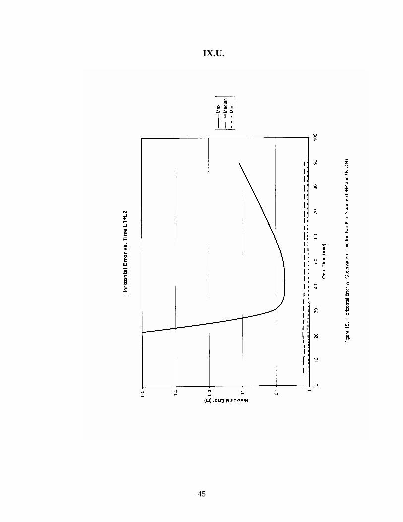
IX.U. Figure 15 - Horizontal Error vs. Observation Time for TwoBase Stations (OHP and UCON) 45

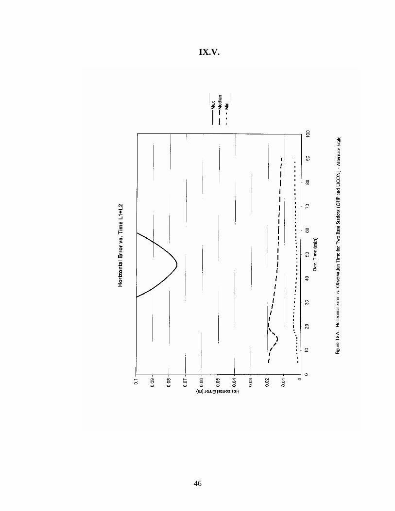
IX.V. Figure 15A - Horizontal Error vs. Observation Time for TwoBase Stations (OHP and UCON) - Alternate Scale 46

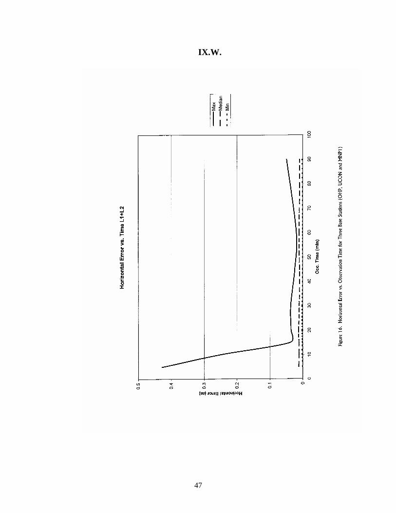
IX.W. Figure 16 - Horizontal Error vs. Observation Time for ThreeBase Stations (OHP, UCON, and MNP1) 47

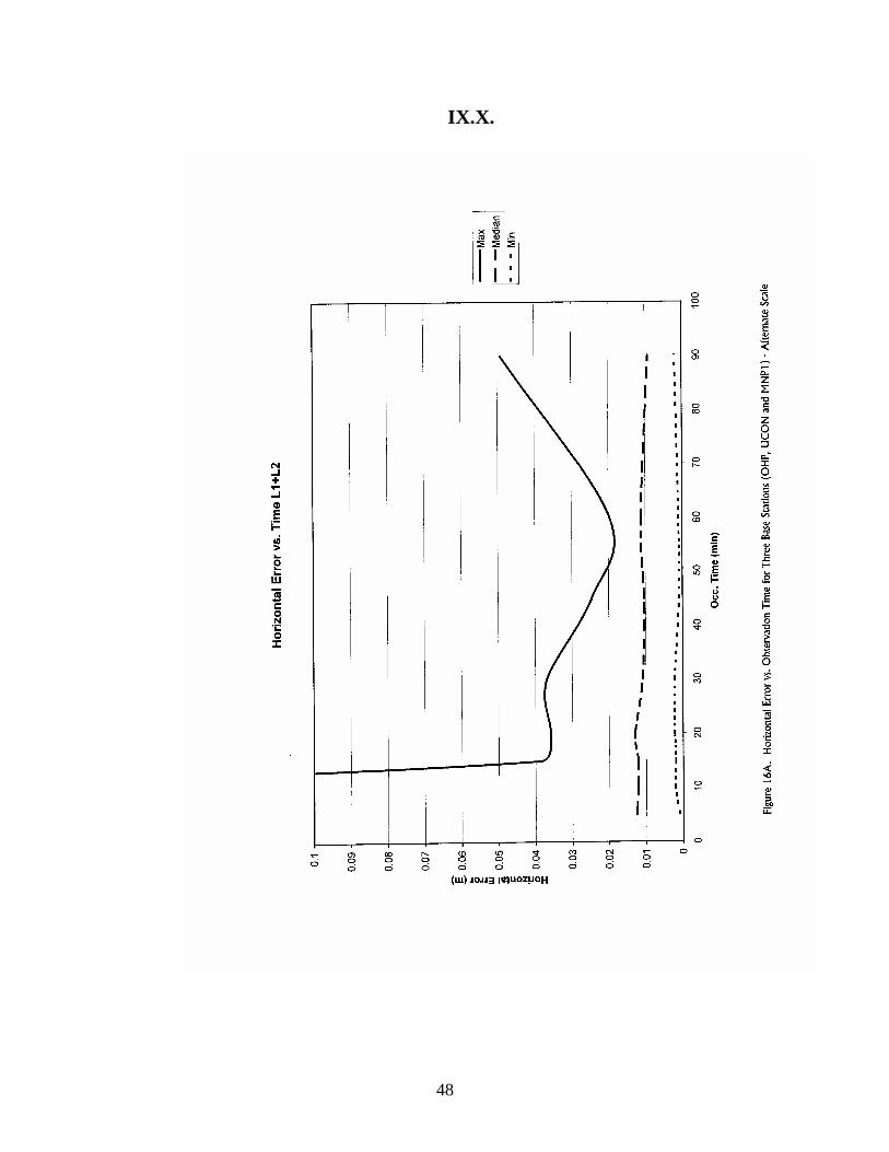
IX.X. Figure 16A - Horizontal Error vs. Observation Time for ThreeBase Stations (OHP, UCON, and MNP1) - Alternate Scale 48

IX.Y. Figure 17 - 5 Minute Observation Horizontal Error vs. DistanceFrom OHP Base Station for Various Combinations of Base Stations 49

IX.Z. Figure 18 - Distribution of Horizontal Error for Varying OccupationTimes 50

IX.AA. Figure 19 - Distribution of Vertical Error for Varying OccupationTimes 51

1

I. INTRODUCTION

The Connecticut Department of Transportation (ConnDOT) operates aGPS base station from their headquarters in Newington, CT, which is centrallylocated for Connecticut users (Figure 1). The base station is known as the OliverH. Paquette base and is abbreviated as OHP Base. Depending on which of twoantennas are mounted on the post, which is fixed in position on the roof of theheadquarters building, ConnDOT's Geodetic Section can provide base stationGPS observations for mapping quality, geodetic quality, or both types of userssimultaneously. The latter capability is accomplished by inserting a signal splitterin the antenna cable (Figure 2). Note that mapping quality observations are alsoreferred to as "code" observations and geodetic quality observations are alsoknown as survey quality observations or "carrier" observations.

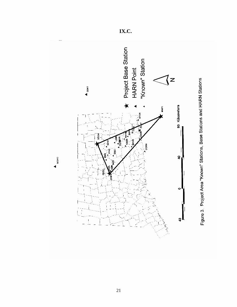
The authors were commissioned by the ConnDOT Joint HighwayResearch Advisory Council (JHRAC) to provide an empirical study of theaccuracy of coordinate positions users may expect when using the ConnDOT basestation for differential GPS operations. The study as initially conceived was tolook at coordinate accuracies with respect to distance from the base station, lengthof observation session, and number of local "known" stations used in conjunctionwith the base station. The authors decided to add a second base station at theUniversity of Connecticut, and use the USCG Montauk Point, Long Island basestation as a third (Figure 3). Note that the distances between the three project basestations are:

OHP to UCON 25.5 milesUCON to MNP1 55.3 milesMNP1 to OHP 61.0 miles.

Coordinate position accuracies using various combinations of the threebase stations, which effectively surround the project area, and observations atlocal "known" stations were examined and analyzed. This report for current andpotential GPS users discusses the results of the study and makes recommendationsfor achieving the desired accuracies of a variety of users.

The method chosen to provide this information about accuraciesattainable, and methods required to obtain these accuracies, was to establish alarge number of High Accuracy Reference Network (HARN) quality points, welldistributed geographically, over southeastern Connecticut. Experimentalobservations were then made on all of these points, using standard satellite signalreception methods, to obtain coordinated positions to compare with the previouslyestablished HARN coordinates. This study concentrates on survey quality signalreceptions. The HARN quality network observations were processed first todetermine the quality of base line solution between stations using the broadcast

2

ephemeris. Those base lines which did not resolve to acceptable quality solutionswere reobserved. Finally, all base line solutions were of acceptable quality. TheHARN network was then reprocessed using the precise ephemeris. The preciseephemeris is obtained from the USCG via the Internet. The Internet site isoperated by the NGS. The final product of this computation was a NAD 83/92,Order B, HARN network, the highest quality network obtainable within theproject and equipment constraints (one part in a million) (previously availableNAD 83 first order control in Connecticut is one part in one hundred thousand).

The experimental observation sets were processed using the broadcastephemeris, as is most commonly the case with ordinary GPS use. The processingyielded coordinates for each of the control stations for observation times of 5, 10,15, 30, 45, 60, and 90 minutes for various combinations of base stations for bothone frequency (L1) and dual frequency (L1 and L2) observations. Thecomputations allowed analysis and charting of the difference in coordinateposition from the HARN coordinates based on 1.) observation time, 2.) distancefrom base station(s), 3.) number of base stations, and 4.) number of receivingfrequencies. The authors used spreadsheet software to compute the positionalvariances and plotted graphs showing the relationships between positional errorand the four variables listed above.

Armed with charts for two full sets of observations at 19 stations, relatingpositional error and the four variables, the analysis of the data was a dauntingexercise. Conclusions regarding the four variables' effect on positional accuracywere made and are reported in detail in the conclusions section.

Definitions of terms which may not be immediately familiar to readers arefound in the Appendix (page 22). Also located in the Appendix is a list ofacronyms used in this report and in common use among GPS professionals (page23).

II. PROJECT DESCRIPTION

II.A. Project Initiation

The project began in 1994 with a conference between project personneland ConnDOT Central Surveys personnel about station selection for the GPSobservations. It was anticipated that the project observations would be useful toCentral Surveys in their maintenance of the Connecticut Coordinate Grid System(CGS) if the stations were chosen wisely. The first thought was that existing CGSstations should be used as project stations. Consequently ConnDOT personnelused their personal recollections of points and station descriptions to select CGSstations in southeastern Connecticut for reconnaissance by project personnel. Theprimary criteria for final project point selection were monument condition andGPS signal access suitability.

3

II.B. Point Reconnaissance

Using compass/clinometer instruments, steel tapes, plumb bobs, shovels,and magnetic locator, project personnel visited each of the CGS stations todetermine their suitability as project GPS points. The CGS station visits yieldedseveral different characteristics for the stations, namely:

1. CGS points destroyed2. CGS points destroyed but had nearby reference marks that were

suitable as project GPS points3. CGS points and/or reference marks recovered, but unsuitable for

GPS observations4. CGS points and/or reference marks recovered but only

marginally suitable for GPS observations5. CGS points recovered and quite suitable for GPS observations.

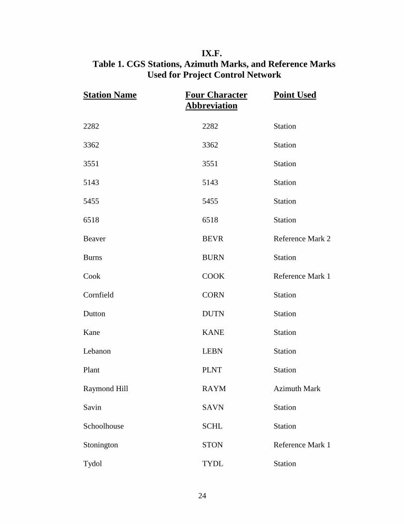
Table 1 is a list of the CGS stations, azimuth marks, and reference marks used forthe project experimental control stations (page 24).

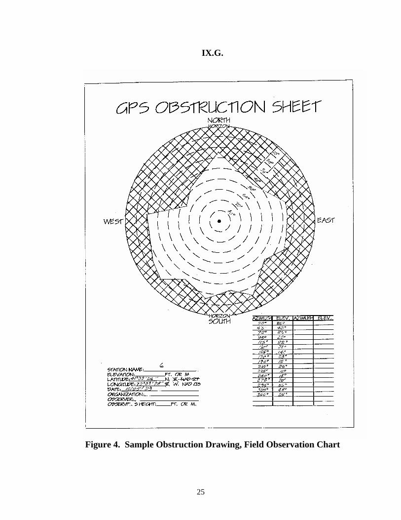
Obstruction drawings were made for each of the suitable and marginallysuitable points and were entered into the mission-planning portion of the GPSprocessing software. Sample obstruction data field charts and GPS planningsoftware drawings are included in the appendix (Figures 4 and 5).

II.C. Project Point Selection

Those points suitable and marginally suitable for GPS observation wereplotted in their proper CGS coordinate positions and examined for suitability asproject points based on a simultaneous evaluation of two factors, 1.) their GPSobservation suitability and 2.) the desirability of spacing for the project. Sixteenpoints were selected to comprise the control network. Three points were addedlater in the project when we decided there were not enough points close to theConnDOT base station (Figure 3).

III. NETWORK OBSERVATIONS

III.A. Communications Problems

One of the first problems encountered in the project was observations notgoing smoothly, in spite of good planning, and the consequent need to reobservethe session. If an adequate means of communicating between stations wasavailable this problem could often be avoided. Typical problems included 1.) notgetting the receiver set up and observing at the prescribed time and 2.) notreceiving signals from the minimum required number of satellites. The firstmethod of communicating between stations in an observation station that was

4

tried was using powerful two-way radios. Two problems were associated with thetwo-way radios: 1.) some two-way radio transmissions interfere with the GPSradio signals and 2.) some of the project control stations are too far apart forcommunication with even the most powerful two-way radios. Our experience wasthat the two-way radio transmission completely blocked the satellite signals,thereby interrupting the observation session each time the two-way radiotransmitter was keyed. This was the case even when the transmitting frequencywas outside those listed in the Trimble report as offending frequencies. Equipment vendors report that the newer chips in the GPS receivers eliminate thisproblem, but those using older receivers must still make sure that two-way radiocommunications do not block their GPS radio waves.

Cellular telephones proved to be a good means of communicating betweenproject observation stations, once certain problems with them were ironed out. The cellular telephone problems encountered were: 1.) batteries that did not lastlong enough for a day's worth of observations and communications, 2.) batterycharger malfunctions, and 3.) coverage range of the cellular telephone company. These problems can generally be avoided by purchasing the right telephones andbatteries and selecting the right cellular telephone company.

III.B. HARN Specifications

Order "A" HARN specifications require setting special new types ofmonuments and observing satellite radio wave signals at each station longer thanwe felt was necessary to obtain the control network accuracy required for thisproject.

Order "B" HARN specifications were generally followed in establishingthe project control network. Order "B" specifications are for a one part in onemillion (1:1,000,000) accuracy standard. We did not do atmospheric conditionmonitoring and did not include the required number of vertical control points(benchmarks) in our network because we felt we would obtain the requirednetwork control accuracy for the project without them. We would like to integratemore benchmarks into the network in the future to see if any significant differencein coordinated position of the 19 stations is effected by the densification ofvertical control points.

III.C. Equipment

Equipment used for field observations consisted of Trimble Navigation,Ltd. 4000SSE dual frequency geodetic receivers and geodetic antennas withground planes. Receivers and antennas used were from the pool of 11 receiversowned by the University of Connecticut (UConn) (4), Central Connecticut StateUniversity (CCSU)(3), and ConnDOT (4).

5

IV. HARN CONTROL SELECTION

Published coordinate values on the CGS are in the process of beingupgraded from the North American Datum of 1927 (NAD27) to the improvedNorth American Datum of 1983 (NAD83). ConnDOT's Central Surveyscontinues to make the field survey measurements to densify the monumentednetwork and the lengthy and complex computations required to publishcoordinates for the entire CGS. In the middle of the five-year recomputationprocess the National Geodetic Survey (NGS) decided that a further improvementof NAD83 was possible and so created a refined NAD83 datum known asNAD83/92. We decided to use the best available datum, NAD83/92, for ourproject. Although it would be a horrendous task for Central Surveys to recomputethe portion of the CGS already upgraded to NAD83, using new GPS observationsand either NAD83/92 or NAD83 values for the HARN control stations fairlyeasily yields coordinate values on either datum for the 19 stations in the projectcontrol network. The NAD83 values were supplied to Central Surveys forpotential use in their CGS network.

IV.A. NGS Control Stations to "Surround" the Project Area

To assign NAD83/92 values to our network, control stations withNAD83/92 values, surrounding our network, had to be determined. The NGSsupplied us with descriptions, coordinates, and elevations of all NGS controlpoints in Connecticut and surrounding states. Four control points were found thatsatisfactorily surrounded our network; two in Connecticut, one in Massachusetts,and one in Rhode Island. The station names are Puglisi, Plant, Mount Holyoke,and Central (Figure 3). The distances between the HARN stations are:

Puglisi to Mount Holyoke 43.6 milesMount Holyoke to Central 62.4 milesCentral to Plant 46.2 milesPlant to Puglisi 41.8 miles.

The base stations at ConnDOT headquarters (OHP) and UConn (UCON)had to be integrated into the project HARN network also since UCON was a newstation and OHP had only NAD83 coordinate values. In order to create therequired base line ties between the project network, the OHP and UCON basestations, and the four HARN stations, nine GPS receivers were required andpersonnel were required to operate each receiver. Four UConn receivers, threeCCSU receivers, and two ConnDOT receivers were used, and since there were notenough project personnel to operate all the receivers, Central Surveys fieldpersonnel operated their receivers plus some of the UConn and CCSU receivers.

6

IV.B. HARN Observations

The observations to tie the project base stations and network stations to theNGS HARN stations were done on two different days consisting of threeobservation sessions each. Six project network stations where multiple base linesintersected were chosen for this purpose. The sketch and explanation below willhelp readers understand how the observation ties to the six network stations, withthe desired base line redundancy, were accomplished with four receivers.

.MOHO

. UCON

.CENTRAL

.PUGLISI.OHP

.A .B

.C .D

.E .F

.PLANT

Day one observations had three two-hour sessions with receivers atPuglisi, MOHO, Central, Plant, and OHP for all sessions and receivers atthe following combinations of stations for

Session One: A,B,C,DSession Two: C,D,E,FSession Three: A,B,E,F

Day two observations came later in the project, after we decided towork with three base stations, rather than with one base station and otherlocal controlling stations. Day two observations were essentially the sameas day one observations with the substitution of base station UCON for basestation OHP.

Figure 6 shows the resulting baselines drawn to scale.

7

The two-hour sessions for days one and two were plannedconsidering the need to move the four receivers at project network stationstwice and to have the moves coincide with periods of low satelliteavailability and/or high positional dilution of precision (PDOP).

Communications for the two days of HARN observations were withthe four project cellular telephones plus one of the student worker's personalcellular telephone and the Central Surveys office telephone, since stationsPuglisi and OHP were close to the Central Surveys office. This is obviouslynot one telephone per station, but with some predetermined plans in theevent any of the stations without telephones had problems, or needed to becontacted, and some improvised leap frog calls when some of the telephoneswere out of range for certain other telephones; the observation sessions wereaccomplished, essentially as planned.

HARN observations within the project control network were madegenerally at three stations at a time and occasionally simultaneously at fourstations. Observation sessions were planned so that all base lines were observedat least once, but most were observed multiple times to provide the redundantmeasurements desired to ensure network accuracy. Observations were made bythe project principal investigators and graduate student, and several undergraduatestudent workers in whatever combinations were available. Occasionalobservations were also made by GPS independent study students from UConn andCCSU.

Some early observations had to be discarded and reobserved due to poormission planning or lack of mission planning, or due to the lack of goodcommunication tools for the observers. Once good cellular telephonecommunications and good mission planning procedures, using individual stationobstruction drawings, were established, project HARN network observations wentsmoothly.

All base lines were processed preliminarily, as described in section V, toverify that they were of acceptable quality. A few base lines did not meet theestablished criteria, so were reobserved and reprocessed until all base lines wereof acceptable quality.

The computational software indicates the type of base line solutionachieved. Only fixed integer solutions were accepted (“ionosphere free fixed” forbaselines longer than 10 kilometers, “L1-only fixed” for shorter baselines). Floatsolutions, in which the integer ambiguity is not fixed, were not acceptable. Ifprocessing yielded only a float solution, the baseline observation data would beexamined and reprocessed using modified parameters and/or controls. If a fixedinteger solution still could not be obtained, the baseline would be reobserved. A

8

discussion of various types of base line solutions is included in the appendix. Seepage 27. The computational software used also provides an analysis of the qualityof the base line computed as well as residual plots for each satellite observed. Two computed quantities are provided as a quality measure for the baselines:"Ratio" and "Reference Variance". The ratio compares the best integer solution tothe second best solution. A high ratio implies that the correct solution wasobtained while a low value indicates uncertainty in the solution. The referencevariance compares the actual variance in the solution to an estimated value. Thelower the reference variance the better. These two measures were used to flagsuspect fixed solutions for further evaluation. The residual plots were very usefulin analyzing problem solutions. If the signal from a particular satellite was noisyor otherwise problematic, the residuals will tend to be high. Oftentimes,removing one problematic satellite observation from the solution, resulted indramatic improvements to the baseline solution.

As we began to do some of the processing of the HARN network, itbecame evident to us that we had not selected enough network stations close tothe OHP base station. Through additional interaction with ConnDOT GeodeticSection personnel and additional field reconnaissance, we were able to identifythree new stations to add to the network. Once observations were made at thenew stations, simultaneously with observations at some of the originally chosenstations, it was felt that we had a suitable network. We were ready to completethe processing and begin the dual set of new observations to evaluate the effect ofseveral parameters on accuracy of computed position of the 19 network stations.

As we proceeded with the creation of our HARN network, discussed thisproject and their proposed new multiple base station project with ConnDOTGeodetic Section personnel, and thought about the later independent observationsof the individual stations, we decided that working with three permanent basestations that surround the project area would better simulate the future GPSoperating conditions in Connecticut than working with the OHP base station andone or more local stations whose positions are known. Consequently, we decidedto establish a new base station at the University of Connecticut (UCON) and usethe United States Coast Guard (USCG) Continuously Operating Reference Station(CORS) at Montauk Point (MNP1) as the third base station. See Figure 3, page21. Integrating the UCON station into the HARN network has been discussed andshown in the earlier sketches of the network. Integration of the Montauk stationinto our HARN network should have been easy, since observation data from thatstation is available over the Internet. We should have been able to simply add thatdata to some of our observation sessions to ensure that we had good, redundantbaseline data connecting our HARN with the CORS station. At this point in time,before there was widespread knowledge about the CORS/HARN shift, wediscovered the discrepancy between CORS and HARN coordinates. We decidedto consolidate the Montauk observations into our observation network to createour own NAD83/92 coordinates for the Montauk base station. An additional

9

complication in using the observations from Montauk Point is that the base stationis an Ashtech receiver while the receivers we are using are Trimble receivers. TheMontauk observations are posted to the Internet in RINEX (receiver independentexchange) format for use in the Trimble processing software. The Montaukstation was added to the HARN primarily by obtaining Montauk observations attimes when our network coastline stations CORN, COOK, PLANT, ANDSTONINGTON were being observed and creating processing baselines betweenMontauk and the coastline stations. The final sketch representing the network tiesto HARN and project base stations is shown below.

.MOHO

. UCON.CENTRAL

.PUGLISI

.OHP.A .B

.C .D.

.E.CORN .COOK .PLANT .F.STONINGTON

.MONTAUK

Figure 7 shows the project base station-HARN tie-in baselines drawn toscale.

V. PROCESSING HARN OBSERVATIONS

The first level of processing was of each session, using the broadcastephemeris which provides the predicted positions of the satellites for any time. For each of these sessions we ensured that all base lines solutions were fixedinteger solutions and that the base lines had acceptable ratios and referencevariances. If there were other observations of the discarded base lines that hadacceptable solutions, the base line was not reobserved. If the discarded base linehad not been acceptably observed as part of another observation session, it wasreobserved. When all base lines had acceptable solutions, we moved on to thenext processing level, using the precise ephemeris, which can be thought of as an“as-built” of the satellite positions for a given time; it is based on actual positionsof the satellites as determined by several tracking stations located across theglobe.

10

The broadcast ephemeris is automatically collected by the GPS receivers. The precise ephemeris may be obtained from NGS using their new “user-friendlyCORS” utility. It is generally available within two days of the observation date.

The processing was done in four sections first, then, when we weresatisfied with the data used in these sessions, all of the acceptable data wasprocessed simultaneously to obtain the final coordinate and elevation values forour experimental 19 station HARN. In this phase of the processing we used onlyindependent base lines.

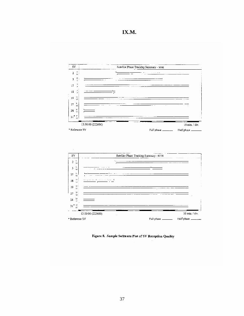
For each processing section we used the processing software's analyticalcapabilities to observe what portion of time each SV was being receivedeffectively by each observation station. Were there cycle slips from the SV, orwere there extensive periods when the SV signals were not being received by thestation? See Figure 8, page 37. If there were significant problems with the signalreceptions from a particular SV then its signals were removed and the processingwas redone. We would like to have been able to simply remove the portion of theSV signals that were problematic from the processing session, but the softwaredoes not have that flexibility. Consequently, long periods of good observationsfrom a particular SV had to be discarded if there were significant periods of poorsignals during an observation session. If the SV removal resulted in too fewsatellites being received during a session or caused PDOP problems, we wentback to the field and re-observed the affected session.

The first processing section contained the four existing HARN stationswhich surrounded the network, OHP base, and the six network stations used to tiethe network to the HARN.

The second processing section contained the four existing HARN stationswhich surrounded the network, UCON base, and the six network stations used totie the network to the HARN.

The third processing section contained all of the observation sessionswithin the 19 station network, including all of the re-observation sessions. Noneof the HARN or base station observations were included in this section.

The fourth processing section contained all of the observation sessionsrequired to integrate the Montauk base station into the HARN

Satisfied that all the observations in the four sections described abovewere good observations, we were ready to process all of the observationssimultaneously, ensure that we had good relationships between all baselines, andfinally, compute coordinates and elevations for the 19 stations to be used forexperimental observations and for the three base stations to be used as fixed

11

control during the experimental observations. The coordinates and elevationswere to be computed by adjusting the observation baselines while holding the fourHARN stations fixed in X, Y, and Z. The four observation sections checked wellindividually and the combined sessions yielded acceptable results. We did notethat there was more adjustment in the long base lines to HARN stationsCENTRAL and MOHO than we liked, particularly vertically. Consequently, inorder to minimize adjustment in the eastern Connecticut network that we wishedto work within, we decided to make our network adjustment holding only the twoHARN stations in close proximity to the 19 station network we wished to workwith, PLANT and PUGLISI, fixed in position (X, Y, Z). This adjustment yieldedthe best available HARN coordinates and elevations for the three base stations and19 network stations we wished to use for our experimental observations. TheNAD83/92 HARN stations we used to establish the coordinates and elevations forour network are part of a 1/1,000,000 control network, while the NAD83 coordinates available for NGS stations in Connecticut and for the OHP basestation are part of only a 1/100,000 control network. Loop closure checkingwithin our network insured that we had a 1/1,000,000 network to use for ourexperimental observations.

VI. EXPERIMENTAL SINGLE SESSIONS

With a good HARN quality network ready to observe on, we began ourexperimental observations. Having learned our lesson about mission planningwell, we used the mission planning software, including the individual stationobstruction drawings in the analysis, and planned when we could make 90 minuteobservations at each station. There were a couple of stations with a lot ofobstructions for which this was impossible and we had to settle for 60 minuteobservations. It was interesting to try to have the poor observation times coincidewith travel time between stations. Depending on travel distance between stationsand the obstructions around the stations, we were able to do three or four stationsper day. On a long day, for example, we were able to observe all of the coastlinestations, STONINGTON, PLANT, COOK, and CORN. We were able in thisinstance to observe the coastline stations in both the order listed above, east towest, and in the reverse order, west to east. This allowed us to be sure that thesatellites forming the observation constellation for the two sets of observationswere different. We decided to make two independent sets of observations of the19 stations in the network and to make sure that the satellite, or SV, configurationwas different for the two observation sessions at each station.

Positions computed for each station were similar for each of theobservation sessions, and the SV configurations were different for the observationsessions, so conclusions drawn from the positions achieved in the experimentalobservations are valid.

12

The parameters affecting position accuracy we wished to evaluate weredistance from base station, number of base stations used, number of receivingfrequencies (L1 alone or L1 and L2), and observation time. Early processingrequired to evaluate these parameters was for observation times of 2, 3, 5, 7, 10,15, 30, 45, 60, and 90 minutes for L1 alone and for L1 and L2. This processingwas done for seven base station combinations: OHP alone; UCON alone; MNP1alone; OHP and UCON; OHP and MNP1; UCON and MNP1; and OHP, UCON,and MNP1. Examples of the charts used to examine these processing results areincluded in the appendix (Figures 9 and 10). Note that after we processed a fewstations it became evident that processing for less than 30 minutes for L1observations yielded no usable coordinates or elevations. A computation wasmade for 10 minutes to demonstrate this, then computations were made for 30, 60,and 90 minutes for analysis. Later processing for L1 and L2 observations was for5, 10, 15, 30, 45, 60, and 90 minutes. This processing was done for OHP alone,OHP and UCON, and OHP, UCON, and MNP1.

A spreadsheet was used to calculate the horizontal and vertical variation incomputed position of each station from the HARN control position. Finally,graphs of the parameters were created to allow analysis of the effect of the fouraccuracy parameters. Samples of these spreadsheet and graphs are included in theappendix and will be referred to individually in the Section VII, "Analysis ofResults of Position Accuracy Computations."

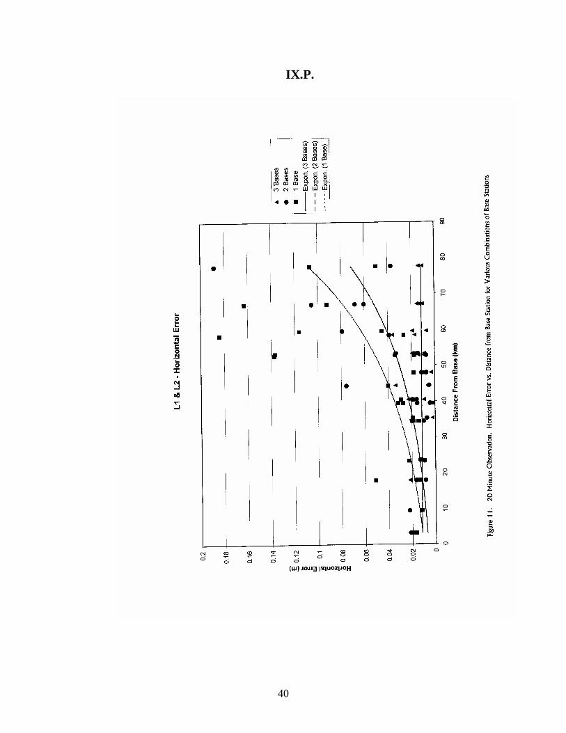
Using one base station and receiving on L1 alone, observation for 60minutes was required to yield 2 centimeter horizontal position accuracy fordistances up to 10 kilometers. Two centimeter vertical accuracy for distances upto 10 kilometers also required 60 minute observation. Receiving on L1 and L2 andusing one base station, 2 centimeter horizontal position accuracy for distances upto 20 kilometers was achieved with observations of only 20 minutes (Figure 11). Vertical accuracy with one base station varied so that no comparable statementcan be made.

Observations using two base stations and dual frequency receivers showsthat 2 centimeter horizontal position accuracy was not achieved when distancesfrom the OHP base stations exceeded 40 kilometers (Figure 11), and 2 centimetervertical accuracy with one base station varied so that no comparable statement canbe made.

For observation of points within a triangle formed by three base stationsseparated from each other by no more than 98 kilometers, distance from basestations does not seem to be a factor for horizontal position or vertical accuracy. This is fortunate as it would be a difficult parameter to analyze. Controlling thecomputed horizontal and vertical position accuracies with three base stationsrequired 60 minutes of observation for 2 centimeter horizontal position accuracy,with no results worse than 3.5 centimeters (Figure 16A), and 60 minutes of

13

observation for 3 centimeter vertical accuracy receiving on L1 anywhere withinthe three base station triangle. Receiving on L1 and L2 reduced the observationtimes to 15 minutes for 1 centimeter horizontal position accuracy and 15 minutesfor 1 centimeter vertical accuracy, with no median results worse than 3.5centimeters horizontally and 4 centimeters vertically (Figures 16A and 12).

VII. ANALYSIS OF RESULTS OF POSITION ACCURACYCOMPUTATIONS

The position accuracy factors we chose to evaluate are interdependent. Discussions of one factor will thus often include discussions of other factors. Theinterdependence of the factors did, however, influence the order in which wechose to discuss them and in some cases caused us to decide to eliminate someobservations from consideration. As the individual factors are discussed, we willindicate situations where findings about one factor are considered irrelevantbecause of findings about another factor.

VIIA. Position Accuracy Factors

We will discuss four factors which affect differentially corrected GPSposition accuracy achieved at a point when using a base station or multiple basestations. The factors are:

1. Single vs. Dual Frequency Observations2. Number of Base Stations3. Duration of Observation4. Distance from Base Station

VII.A.1. Single vs. Dual Frequency Considerations

A look at Figures 9 and 10 will be useful in considering the positionalaccuracy effect of single vs. dual frequency GPS observations. The results of thecomputations from these observations are typical of those found throughout the 19station experimental network. These observations are for station Stonington(STON). The three numbers in the upper left hand corner in the box with thestation name are the NAD 83/92 HARN quality coordinates (Northing andEasting) and ellipsoid height in meters. For the coordinates we have shown onlythe units place and four decimal places to avoid a lot of needless writing ofnumbers. The numbers in each box are the computed values of the coordinatesand ellipsoid height for the observation time and base station combination listed.

It is obvious that we do not approach 2 centimeter accuracy in eitherhorizontal or vertical position for observations of less than 30 minutes whenobserving on only the L1 frequency. Yet when observing with both the L1 and theL2 frequency, we approach 2 centimeter accuracy in both horizontal and vertical

14

position after only 5 minutes of observation. Although dual frequency receiverscost more than single frequency receivers, the cost differential is not enough to notwarrant purchasing dual frequency and thereby saving about a half hour ofobservation time at every station for which coordinates or elevations are desired. We will consequently limit the major portion of our discussion of the other threeaccuracy factors to observations with dual frequency receivers.

VII.A.2. Number of Base Stations

Examination of Figures 11 and 12 illustrates the telling point about thenumber of base stations used very well. We have chosen to examine horizontaland vertical errors found in 20 minute observations on a plot of error versusdistance from the OHP base station for one, two, and three base stations heldfixed in horizontal and vertical position. From these graphs we can see thathorizontally and vertically, the error increases with distance from the base stationwhen one or two base stations are used, but that the error is essentially unchangedfrom 0 to 80 kilometers with three base stations. That median error is a veryacceptable 1 centimeter. Note that for the 20 minute observation data chosen asan example, for one base station, observations further than 20 kilometers fromOHP cannot produce position accuracy better than 2 centimeters horizontally. Fortwo base stations, the distance from OHP can extend to 40 kilometers for 2centimeter horizontal accuracy.

The number of base stations is also a factor in the required observationtime, as will be discussed in the next section. In addition to the positiveinteractions observations from three base stations (surrounding the project area)have with distance and time factors, these observations provide very valuablequality checks of the base lines in the least squares adjustments made by theposition computational GPS software. These checks are unavailable if only onebase station is used and are of limited reliability with two base stations.

VII.A.3. Duration Considerations

Figure 13 shows the median horizontal error for all dual frequencyobservations for various observation times. Note that there is no consideration ofdistance from base station in these graphs. We can see that using one base station,and a minimum observation time of 20 minutes, errors range from 2 to over 3centimeters, with slight improvement over time. This approaches acceptablequality geodetic work. Using the same 20 minute minimum observation time andusing two base stations, the results improve to errors ranging from about one tojust under 2 centimeters, once again seeming to improve with time. With threebase stations, however, from 5 minutes to 90 minutes, the error hovers rightaround an acceptable error of 1 centimeter, with once again some improvementover time. The improvement here is academic, since the 5 minute error is withinthe acceptable range.

15

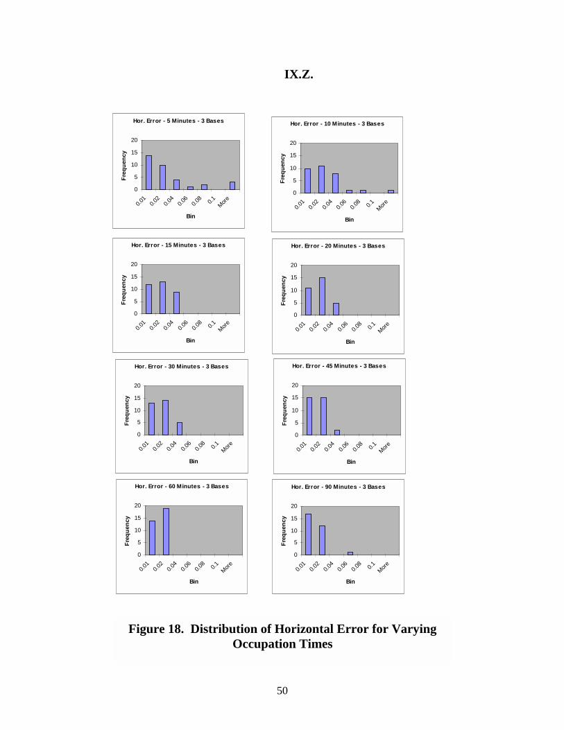
A close look at some of the graphs we have produced reveals that there issome variation in errors from station to station, yielding some scatter in theindividual points from which the smooth exponential curves fit to the data aredrawn. Figures 14 through 16A are designed to allow us to think about this a bit. These graphs look at median, minimum, and maximum errors versus time for one,two, and three base stations. An important observation from these graphs is thatthe variation between the median, minimum, and maximum errors is verysignificantly minimized when using three base stations. For observations wherethe results must always be within the centimeter range, three base stations must beused. Note on Figure 14 that errors of 2 to 3 decimeters were experienced evenwhen the observations were in the 30 to 60 minute range with only one basestation and for two base stations the errors observed were in the 1 to 2 decimeterrange. With three base stations, however, the maximum errors were generally inthe 4 to 6 centimeter range. Figures 12 and 19 clearly show the improvement indistribution of horizontal and vertical error respectively with increasedobservation time.

VII.A.4. Distance Considerations

We may revisit Figures 11 and 12 to consider the effect of distance on thehorizontal and vertical position accuracy achieved from GPS observations. InSection VIIA.2, Number of Base Stations, we made the following statements. "Note that for the 20 minute observation data chosen as an example, for one basestation, observations further than 20 kilometers from OHP cannot produceposition accuracy better than 2 centimeters horizontally. For two base stations,the distance from OHP can extend to 40 kilometers for 2 centimeter horizontalaccuracy, but only to 25 kilometers for 2 centimeter horizontal accuracy." Noteagain that for the entire range of distances from OHP (0 to 80 kilometers), theposition error for points "surrounded" by the three base stations is essentially aconstant 1 centimeter. Similar graphs were produced for other observation timesand yielded slightly different results. For example, for a 5 minute observation, 2centimeter horizontal accuracy can be expected for only up to 17 kilometers withone base station and 30 kilometers with two. Three base stations yield 1 to 2centimeter accuracy from 0 to 80 kilometers in 5 minutes. These results are allslightly worse than for the 20 minute observation, which is expected, but showsimilar results regarding the relationship between distance from base station andpositional accuracy.

VIII. CONCLUSIONS AND RECOMMENDATIONS

GPS is an excellent geodetic control survey tool, when used properly. When improperly used, erroneous horizontal and vertical positions of controlpoints can be proliferated and used to their great detriment by the unsuspectingsurveyor or mapper and their clients. GPS can be used effectively and properly or

16

it can be misused. Effective, proper use can be very profitable while improper usecan simply minimize the available business profit or time savings, or it can causea large sequence of problems having domino-like effect on many subsequent usersof inaccurate control points.

GPS is very accurate. Inaccuracies can result from problems with the toolsGPS receivers interact with, such as the tribrachs and tripods the receivers aremounted on to be positioned over control points. It is essential to keep thetribrachs calibrated and the tripods tight.

The importance of mission planning cannot be overstressed. GPSobservations when the proper number of or configuration of satellites are notavailable are worthless and can be easily avoided by proper mission planning.

Mission planning comprises more than obstruction drawings and numberof satellite and PDOP plots. Missions can be aborted at cost of time and moneyfor other failures, such as not having enough GPS receiver batteries charged forthe planned observation time, failing to have the cellular telephone or two-wayradio batteries charged, not having a tribrach in the GPS receiver case, not havinga tripod in the truck, sending an operator to a station that he or she has not seenbefore and consequently cannot find, or failing to ensure that the base station youare planning to use will be operating when you want to use it.

When observations at multiple stations must be coordinated,communications between the operators at the stations are essential. Cellulartelephones have proven to be very effective, particularly when distances betweenstations are greater than the range of two-way radios. Two-way radios should beused cautiously because of the potential for interference with GPS satellite radiosignals.

Dual frequency geodetic receivers allow much shorter observation timesthan single frequency receivers for centimeter accuracy horizontal and vertical. The higher cost of the dual frequency receivers can easily be recouped in a shorttime by their greater production.

Whenever possible, GPS observations should be conducted within an areasurrounded by at least three base stations. This eliminates effects of time anddistance on the accuracy of horizontal and vertical positions achieved from GPSobservations. Centimeter accuracy is achieved in observations of 20 minutes orless. For situations where lesser accuracy is required, observations can be shorter. Five centimeter accuracy can be achieved in 5 minutes of observation.

The foresight of Central Surveys personnel in proposing a nine-stationbase station network for Connecticut provides a tremendous benefit to all futureGPS users in Connecticut. Once the nine base stations are in place, GPS users

17

will be able to complete control surveys anywhere in Connecticut with therequisite minimum of three base stations.

18

IX. APPENDIX

19

IX.A.

20

IX.B.

Figure 2. OHP Base Station Schematic

Geodetic AntennaCONNDOT Roof

PathFinder AntennaGenerally

AutomaticallyZipped intoFiles Hourly

PathFinderBase Station

Signal Splitter

4000SSEReceiver

PublicDirectory

One Month ofFiles

Modem

UserCommunity

21

IX.C.

22

IX.D.

GLOSSARY OF TERMS USED IN THIS REPORT

Base Station – a continuously operating GPS receiver referenced to a known

point.

Broadcast Ephemeris – the ephemeris transmitted to the GPS user as part of the

data message of the GPS signal (See also Ephemeris and Precise Ephemeris)

Differential Positioning – precise measurement of the relative positions of two

receivers tracking the same GPS signals simultaneously

Ephemeris – the predictions of satellite position as a function of time (See also

Broadcast Ephemeris and Precise Ephemeris)

Global Positioning System – a navigational/positioning system based on the US

Department of Defense’s NAVSAT orbital satellite system.

HARN – High Accuracy Reference Network – A network of highly accurate

monumented locations determined by the US National Geodetic Survey using an

extensive network of GPS baselines.

Positional Accuracy – Closeness of position derived from test occupations at a

point to the position of that point determined from the HARN-quality network

Precise Ephemeris – A “post-fit” ephemeris based on earth observation of actual

satellite orbits (See also Ephemeris and Broadcast Ephemeris)

23

IX.E.

ACRONYMS USED IN THIS REPORT

CCSU Central Connecticut State UniversityCGS Connecticut Grid System or Connecticut Coordinate

SystemConnDOT Connecticut Department of TransportationCORS Continuously Operating Reference Station (GPS)DOP Dilution of Precision (from many causes in GPS work, see

PDOP)GPS Global Positioning SystemJHRAC Joint Highway Research Advisory Council (ConnDOT and

UConn Civil and Environmental Engineering Department)HARN High Accuracy Reference NetworkMNP1 The four character name for the USCG CORS base station

at Montauk Point, Long Island, NYNAD North American Datum (year specific, NAD 27 coordinates

do not mix with NAD 83 coordinates in the traditionalapples and oranges example way)

NAD 27 North American Datum of 1927 (used exclusively of lateuntil, 1983, still used in the majority of cases today,although we are slowly converting to NAD 83)

NAD 83 North American Datum of 1983 (uses an upgraded spheroidfrom NAD 27)

NAD 83/92 North American Datum of 1983 upgraded in 1992NGS National Geodetic SurveyOHP or OHP Base The Oliver H. Paquette Base Station at ConnDOT headquarters in Newington, CTPDOP Positional Dilution of Precision (one of the many potential

causes of error in GPS work. This one is caused by therelative position of the satellites, or space vehicles, to thereceiving GPS antenna)

RINEX Receiver Independent Exchange FormatSV Space Vehicle. One of the constellation of Navstar

satellites that comprise the GPSUCON The four character name for the base station created for this

project. It is located on the roof of the Life SciencesBuilding Annex.

UConn The University of ConnecticutUSCG United States Coast Guard

24

IX.F. Table 1. CGS Stations, Azimuth Marks, and Reference Marks

Used for Project Control Network

Station Name Four Character Point Used Abbreviation

2282 2282 Station

3362 3362 Station

3551 3551 Station

5143 5143 Station

5455 5455 Station

6518 6518 Station

Beaver BEVR Reference Mark 2

Burns BURN Station

Cook COOK Reference Mark 1

Cornfield CORN Station

Dutton DUTN Station

Kane KANE Station

Lebanon LEBN Station

Plant PLNT Station

Raymond Hill RAYM Azimuth Mark

Savin SAVN Station

Schoolhouse SCHL Station

Stonington STON Reference Mark 1

Tydol TYDL Station

25

IX.G.

Figure 4. Sample Obstruction Drawing, Field Observation Chart

26

IX.H

Figure 5. Sample Obstruction Drawing, Software Plotting

27

IX.I.

Base Line Solutions Discussion

32

IX.J.

Ratio and Variance Discussion

35

IX.K.

36

IX.L.

37

IX.M.

38

IX.N.

Figure 9. Sample Processing Results Chart for L1 Observations

39

IX.O.

Figure 10. Sample Processing Results Chart for L1 and L2Observations

40

IX.P.

41

IX.Q.

42

IX.R.

43

IX.S.

44

IX.T.

45

IX.U.

46

IX.V.

47

IX.W.

48

IX.X.

49

IX.Y.

50

IX.Z.

Hor. Error - 5 Minutes - 3 Bases

0

5

10

15

20

0.01

0.02

0.04

0.06

0.08 0.1 More

Bin

Freq

uenc

yHor. Error - 10 Minutes - 3 Bases

0

5

10

15

20

0.01

0.02

0.04

0.06

0.08 0.1 More

Bin

Freq

uenc

y


0

5

10

15

20

0.01

0.02

0.04

0.06

0.08 0.1 More

Bin

Freq

uenc

y


0

5

10

15

20

0.01

0.02

0.04

0.06

0.08 0.1 More

Bin

Freq

uenc

y


0

5

10

15

20

0.01

0.02

0.04

0.06

0.08 0.1 More

Bin

Freq

uenc

y


0

5

10

15

20

0.01

0.02

0.04

0.06

0.08 0.1 More

Bin

Freq

uenc

y


0

5

10

15

20

0.01

0.02

0.04

0.06

0.08 0.1 More

Bin

Freq

uenc

y


0

5

10

15

20

0.01

0.02

0.04

0.06

0.08 0.1 More

Bin

Freq

uenc

y

Figure 18. Distribution of Horizontal Error for VaryingOccupation Times

51

IX.AA

Vert. Error - 05 Minutes - 3 Bases

0

5

10

15

20

0.01

0.02

0.04

0.06

0.08 0.1 More

Bin

Freq

uenc

y


0

5

10

15

20

0.01

0.02

0.04

0.06

0.08 0.1 More

Bin

Freq

uenc

y


0

5

10

15

20

0.01

0.02

0.04

0.06

0.08 0.1 More

Bin

Freq

uenc

y


0

5

10

15

20

0.01

0.02

0.04

0.06

0.08 0.1 More

Bin

Freq

uenc

y


0

5

10

15

20

0.01

0.02

0.04

0.06

0.08 0.1 More

Bin

Freq

uenc

y


0

5

10

15

20

0.01

0.02

0.04

0.06

0.08 0.1 More

Bin

Freq

uenc

y


0

5

10

15

20

0.01

0.02

0.04

0.06

0.08 0.1 More

Bin

Freq

uenc

y


0

5

10

15

20

0.01

0.02

0.04

0.06

0.08 0.1 More

Bin

Freq

uenc

y

Figure 19. Distribution of Vertical Error for VaryingOccupation Times

effective use of the conndot gps base stationdocs.trb.org/00938137.pdfeffective use of the conndot...

Documents