effective monitoring for biodiversity conservation562951/s4300559_final_thesis.pdf · eve...

Effective monitoring for biodiversity conservation

Payal Bal

B.Sc. (Honours), M.Sc., M.Res.

A thesis submitted for the degree of Doctor of Philosophy at

The University of Queensland in 2016

School of Earth and Environmental Sciences

ii

Abstract

Monitoring of biodiversity is expensive and can detract resources for managing biodiversity. Given

limited resources for conservation, it is not only important to assess the choices we make for

managing biodiversity but also those for monitoring biodiversity. This entails considering the

benefits and costs of alternative monitoring strategies, and selecting the ones that best inform and

improve management decisions. However, understanding which aspects of an ecosystem to monitor

(e.g. which species, threat, or indicator) to make effective management decisions is a challenging

task. This is especially true when we are faced with large uncertainties, such as those regarding the

drivers of change when species are impacted by multiple threats. Although optimal monitoring

approaches for conservation decision-making under limited resources have gained popularity over

the last decade, similar approaches for monitoring and indicator selection to inform the

management of multiple threats for biodiversity have received relatively little attention. In this

thesis, I contribute to the theory and tools for selecting monitoring strategies and indicators to

improve management decisions, with a focus on multi-species, multi-threat systems. The four

objectives of my thesis are: (1) to review current approaches for selecting indicator species for

biodiversity management; (2) to assess the value of monitoring species for managing multiple

threats; (3) to assess the relative influence of uncertainty and expected benefits of management on

monitoring decisions for multiple threats; and (4) to develop a simple indicator selection tool based

on a return on investment framework for managing multi-species, multi-threat systems.

The thesis starts with a systematic review of the conservation literature, in chapter two, to assess

the extent to which the selection of indicator species for biodiversity management explicitly

considers management objectives and the management outcomes of monitoring. I find that most

indicator selection studies focus on improving the monitoring efficiency rather than the

management effectiveness, potentially leading to ineffective indicators. Recommendations are

provided to improve indicator selection for management decision-making. I also propose a decision

framework for selecting indicator species and identify decision-analytic approaches to evaluate

alternative monitoring choices that are further developed in the remainder of the thesis.

In chapter three, I use value of information analysis to investigate how monitoring alternative

species subject to multiple threats improves our ability to inform the management of these threats.

iii

Specifically, I compare the effectiveness of different monitoring approaches to learn about the

threats i.e. monitoring just species and monitoring with experimental manipulation of threats. My

results show that monitoring species alone is unlikely to provide useful information for threat

management when there is uncertainty about the effect of multiple threats. Instead, an experimental

design to learn about how species respond to threats in the system provides much higher benefits

for management in terms of conservation outcomes.

In chapter four I again use value of information analysis to establish the benefit of monitoring to

resolve uncertainty about the effectiveness of management on two different threats. Here, look at

the effect of uncertainty versus the relative expected effectiveness of each management action on

the value of monitoring to inform management. I find that decisions regarding whether managers

should implement monitoring to inform management of the threats depend on the difference in the

expected benefit of managing each threat, and the uncertainty in the benefit of managing the threat.

In cases where monitoring is found to be beneficial, monitoring the action with the greater

uncertainty always provides higher benefit.

In chapter five, I propose a relatively simple indicator selection tool for real-world conservation

decision-making, compared to the value of information approach. Here, I evaluate the cost-

effectiveness of alternative indicators for informing management decisions. The approach

incorporates six key factors that include monitoring efficiency, management outcomes and

economic constraints. I find that that indicator selection based on the cost-effectiveness approach

improves threat management decisions when resources are limited, leading to better conservation

outcomes. Because this framework accounts for multiple criteria, it improves on common

approaches whereby indicators are often selected based only on whether they are sensitive to

change, or cheap to monitor.

This thesis makes original contributions to the field of optimal monitoring to manage multi-species,

multi-threat systems. It develops the underlying theory for relatively complex systems where there

is a wide range of possible monitoring options, and proposes decision-analytic approaches to

evaluate alternative monitoring choices. Through the use of case studies, I illustrate different

scenarios of decision making that vary in context, to demonstrate the real world applicability for the

proposed approaches. In doing so, this thesis addresses the repeated calls for monitoring to be better

suited for informing policy and decisions on management actions for biodiversity conservation.

iv

Declaration by author

This thesis is composed of my original work, and contains no material previously published or

written by another person except where due reference has been made in the text. I have clearly

stated the contribution by others to jointly authored works that I have included in my thesis.

I have clearly stated the contribution of others to my thesis as a whole, including statistical

assistance, survey design, data analysis, significant technical procedures, professional editorial

advice, and any other original research work used or reported in my thesis. The content of my thesis

is the result of work I have carried out since the commencement of my research higher degree

candidature and does not include a substantial part of work that has been submitted to qualify for

the award of any other degree or diploma in any university or other tertiary institution. I have

clearly stated which parts of my thesis, if any, have been submitted to qualify for another award.

I acknowledge that an electronic copy of my thesis must be lodged with the University Library and,

subject to the policy and procedures of The University of Queensland, the thesis be made available

for research and study in accordance with the Copyright Act 1968 unless a period of embargo has

been approved by the Dean of the Graduate School.

I acknowledge that copyright of all material contained in my thesis resides with the copyright

holder(s) of that material. Where appropriate I have obtained copyright permission from the

copyright holder to reproduce material in this thesis.

v

Publications during candidature

Refereed journal articles:

Maxwell, S., Rhodes, J.R., Bal, P., Bunnefeld, N., Earle, S., Jones, J.P.G., Knight, A.T., Nuno, A.,

Watson, J.E.M., Milner-Gulland, E.J. (2014) Sustainability: root targets in consensus. Nature, 514,

434-434.

Maxwell, S.L., Milner-Gulland, E.J., Jones, J.P.G., Knight, A.T., Bunnefeld, N., Nuno, A., Bal, P.,

Earle, S., Watson, J.E.M. & Rhodes, J.R. (2015) Being smart about SMART environmental targets.

Science, 347, 1075-1076.

Conference abstracts:

Bal et al. (2016) Selecting indicators for conservation. Society for Conservation Biology – Oceania

Section. Brisbane, Australia.

Bal et al. (2015) Indicator selection for biodiversity management: What are we doing wrong?

International Congress on Conservation Biology. Montpellier, France.

Bal et al. (2015) Benefit of monitoring for conservation decision-making. Centre for Excellence in

Environmental Decisions. Brisbane, Australia.

Bal et al. (2014) Selecting cost-effective indicators to inform management. Society for

Conservation Biology. Kuala Lumpur, Malaysia.

Bal et al. (2014) Selecting indicator species to inform management of multiple threats. Ecological

Society of Australia. Alice Springs, Australia.

Publications included in this thesis

None.

vi

Contributions by others to the thesis

This thesis consists of four manuscripts that have been submitted or are intended for submission for

publication, with myself as the primary author. Chapter two and three are currently in review, and

chapters four and five are working papers that will be submitted for publishing hereafter. These

manuscripts are reproduced as chapters 2 – 5 of this thesis and are written in the plural first-person

pronoun “we” as is customary for publications with multiple authors. In chapters 1 and 6, I use the

singular first-person pronoun “I” as these were written entirely by me, with only editorial input

from my supervisors. Michelle Baker did chapter header illustrations.

Chapter one

This chapter was entirely written by the candidate with input from Jonathan Rhodes and Ayesha

Tulloch.

Chapter two

This chapter is taken from a manuscript prepared by the candidate, Ayesha Tulloch, Prue Addison,

Eve McDonald-Madden and Jonathan Rhodes, which is under review in Frontiers in Ecology and

the Environment. The candidate and Jonathan Rhodes conceived the idea for this chapter. The

candidate carried out the literature review and analysis with advice from Jonathan Rhodes and

Ayesha Tulloch. Prue Addison and Eve McDonald-Madden provided helpful comments on the

decision framework discussed in this chapter. The candidate wrote the manuscript, with editorial

input from all the authors. All other minor contributions are described in the acknowledgment

section of the manuscript.

Chapter three

This chapter is taken from a manuscript prepared by the candidate, Ayesha Tulloch, Iadine Chadès,

Josie Carwardine, Eve McDonald-Madden, Jonathan Rhodes, which is under review in Methods in

Ecology and Evolution. The candidate, Jonathan Rhodes and Eve McDonald-Madden, conceived

the idea for this chapter. The candidate developed the models used in the optimisation and

conducted the analysis, with advice from Jonathan Rhodes. Ayesha Tulloch and Iadine Chadès

reviewed the model and provided helpful comments. Ayesha Tulloch and Josie Carwardine

provided the case study data. The candidate wrote the manuscript, with editorial input from all the

vii

authors. All other minor contributions are described in the acknowledgment section of the

manuscript.

Chapter four

This chapter is being prepared for submission to Ecological Applications. The candidate developed

the ideas for this chapter in collaboration with Jonathan Rhodes, Mick McCarthy and Matt Holden.

The candidate developed the models used in the optimisation, with advice from Jonathan Rhodes,

Mick McCarthy and Matt Holden, and conducted the analysis. Alana Moore reviewed the model

and provided helpful comments. Ayesha Tulloch provided the case study data. The candidate wrote

the chapter, with editorial input from Jonathan Rhodes. All other minor contributions are described

in the acknowledgment section of the manuscript.

Chapter five

This chapter is being prepared for submission to Methods in Ecology and Evolution. The candidate

developed the idea for this chapter with input from Eve McDonald-Madden, Hugh Possingham,

Josie Carwardine, Edward Game, Tara Martin and Ayesha Tulloch. The candidate developed the

cost-effectiveness framework in collaboration with Eve McDonald-Madden, Hugh Possingham,

Josie Carwardine and Jonathan Rhodes. The candidate conducted the analysis. The candidate wrote

the chapter, with editorial input from Jonathan Rhodes, Eve McDonald-Madden, Hugh Possingham

and Josie Carwardine. All other minor contributions are described in the acknowledgment section

of the manuscript.

Chapter six

This chapter was entirely written by the candidate with input from Jonathan Rhodes, Eve

McDonald-Madden and Ayesha Tulloch.

Statement of parts of the thesis submitted to qualify for the award of

another degree

None.

viii

Acknowledgements

For me, this PhD has been much more than the making of this thesis. I have had the opportunity to

travel to a spectacular country, make new friends who I will cherish forever and develop invaluable

professional associations along the way.

There are a number of people I would like to thank, even if most of them will never ever read this.

First and foremost, I would like to thank my supervisor, Jonathan Rhodes. I couldn’t have asked for

a better teacher, mentor, critic, co-author and researcher to guide me though my PhD. Thank you

for taking me on as your student, for being so patient as I learned the ropes, for being so thorough in

your feedback and for always making the time to help. Ayesha Tulloch, thank you for your ideas,

advice and enthusiasm (and data!). Eve McDonald-Madden, thank you for always being

encouraging and supportive, and helping me stay sane. I truly value your advice, be it for work or

regarding life in general. I am grateful to all of you for your guidance over these past years. I am

also grateful to Hugh Possingham, Patrick Moss and Karen McNamara for their support as

reviewers and co-ordinators in milestone evaluations.

I thank the professional staff at the School of GPEM: Judy, Claire, Lorraine, Genna, Suhan, Lia,

Christina, Nivea, Alan, Eros and Jurgen. You have all helped make my PhD experience as effortless

as possible and I thank you whole-heartedly for it. A special mention for Judy Nankiville for

everything that she does for the PhD students at GPEM. Where would we be without you, Judy!

Nathalie Butt and Duan Biggs, thanks for all your advice and encouragement in the last year. To all

my friends, who helped with editing and reviewing parts of this thesis, thank you.

I would like to acknowledge the organisations that have funded my research: the University of

Queensland for my scholarship, and the Australian Research Council Centre of Excellence in

Environmental Decisions and the School of GPEM research grant for the top-ups, travel awards and

general logistical support.

I have been very fortunate to be a part of a number of exceptional research groups: Rhodes

Conservation Research Group, the McDonald-Madden Lab, Landscape Ecology and Conservation

ix

group at GPEM and the Centre for Applied Environmental Decision Analysis. I am honoured to be

accommodated amongst such bright minds and I thank you all for creating an engaging, open and

diverse work environment. I am also grateful to have had the opportunity to visit a number of

research groups in Australia and abroad and would like to thank all the people who have hosted me:

Mick McCarthy and Pauline Byron at the University of Melbourne (Australia); Ben Collen and

Chris Langridge at University College London (UK); E.J. Milner-Gulland and Diana Anderson at

Imperial College London (UK); Yash Veer Bhatnagar and Kulbhushansingh Suryawanshi at Nature

Conservation Foundation (India); and Swapnil Chaudhari at ICIMOD (Nepal). I thank the many

wonderful people for their time and discussions regarding my research at these institutions and at

the Zoological Society of London (UK), UNEP-WCMC (UK), UNEP (UK), Birdlife International

(UK), the University of Cambridge (UK), Indian Institute of Science (India), and the National

Centre for Biological Sciences (India).

This thesis would not have been possible, were it not for my friends in Australia: my newfound

sisters Sylvaine, Abbey and Kiran; my office and lunch mates Jeremy, Rebecca and Rowan; and my

eccentric and dear Australian family Guia, Ezgi, Will, Alvaro, Missaka, Lincoln, Matt and Erin,

Alex, Toby, Xyomara, Justine, Daniel and Roxy! Saori, thanks for making the lead up to thesis

submission much more interesting by showing me around Kyoto. And Ascelin, thank you for

making sure I always had whatever I needed to focus on my work, reading over my drafts, helping

me out of every little PhD-crises and for being so patient.

Finally, I would like to thank my family in India who might have doubted but never once

discouraged. I love you all to pieces. To Mummy and Daddy, thank you for giving us everything. To

Papa, thank you for always being there for us, in spite of the hardships you’ve faced. To Aman,

you’re an amazingly strong woman and I admire you for it. To Rana and Bina, thank you for all

your love. To Ameta and Ekadish, japphi! Q and Paryn, it’s your turn next. To Kunal and Varun for

keeping the sisters sane! To Anuraag, for always replying to my panic messages. To our doggies,

Bruno, Kody and Zorro, because you’ve kept us together and loved.

Nimmi mummy, make way for another PhD in the house. And Daddy, this is dedicated to your

eternal sunshine. I know you both would be proud.

x

Keywords

Optimal monitoring, indicator selection, conservation, decision framework, costs, benefits,

management, decision theory, value of information, cost-effectiveness

Australian and New Zealand Standard Research Classifications

(ANZSRC)

ANZSRC Code Area of Research Precent contributed

050206 Environmental Monitoring 60%

050202 Conservation and Biodiversity 20%

050211 Wildlife and Habitat Management 20%

Fields of Research (FoR) Classification

FoR Code Area of Research Precent contributed

0502 Environmental Science and Management 80%

0102 Applied Mathematics 20%

xi

Table of Contents

Abstract .................................................................................................................................... ii

Declaration by author .............................................................................................................. iv

Publications during candidature ............................................................................................... v

Publications included in this thesis .......................................................................................... v

Contributions by others to the thesis ....................................................................................... vi

Statement of parts of the thesis submitted to qualify for the award of another degree .......... vii

Acknowledgements ............................................................................................................... viii

Keywords ................................................................................................................................. x

Australian and New Zealand Standard Research Classifications (ANZSRC) ......................... x

Fields of Research (FoR) Classification .................................................................................. x

Table of Contents .................................................................................................................... xi

List of Figures ........................................................................................................................ xv

List of Tables ........................................................................................................................ xvi

List of abbreviations ............................................................................................................ xvii

Glossary ............................................................................................................................... xvii

Chapter one – General introduction .................................................................................... 2

Thesis aims and overview ................................................................................................... 16

Chapter two – Selecting indicator species for biodiversity management ....................... 20

Abstract .............................................................................................................................. 20

Introduction ........................................................................................................................ 21

Methods .............................................................................................................................. 25

Results ................................................................................................................................ 30

Discussion .......................................................................................................................... 35

Acknowledgements ............................................................................................................. 39

xii

Chapter three – The value of monitoring species to manage multiple threats ............... 41

Abstract .............................................................................................................................. 41

Introduction ........................................................................................................................ 42

Methods .............................................................................................................................. 44

A stylised multi-species multi-threat system .................................................................. 44

The decision problem ..................................................................................................... 46

Value of information analysis ......................................................................................... 47

Scenario and sensitivity analysis .................................................................................... 49

Case studies .................................................................................................................... 49

Results ................................................................................................................................ 51

Discussion .......................................................................................................................... 56


Chapter four – Uncertainty and the value of information for threat management ...... 63

Abstract .............................................................................................................................. 63

Introduction ........................................................................................................................ 64

Methods .............................................................................................................................. 66

Model of one-species two-threat system ........................................................................ 66


Value of information ...................................................................................................... 68

Benefit of monitoring different management actions ..................................................... 70

Multiple species systems: Fitz-Stirling case study ......................................................... 71

Results ................................................................................................................................ 73

Discussion .......................................................................................................................... 79


xiii

Chapter five – Cost-effective monitoring to trigger conservation interventions ........... 86

Abstract .............................................................................................................................. 86

Introduction ........................................................................................................................ 87

Methods .............................................................................................................................. 89


Cost-effective analysis framework ................................................................................. 90

Six factors for indicator selection ................................................................................... 93

Case Study ...................................................................................................................... 97

Sensitivity analysis ....................................................................................................... 100

Results .............................................................................................................................. 103

Discussion ........................................................................................................................ 108

Acknowledgements ........................................................................................................... 113

Chapter six - Discussion .................................................................................................... 115

Synthesis ........................................................................................................................... 115

Overarching Contributions .............................................................................................. 118

Limitations and future research ....................................................................................... 120

Bibliography ........................................................................................................................ 126

Appendices ........................................................................................................................... 146

Appendix 1: Supporting information for Chapter 2 ......................................................... 146

Appendix 1.1: Review methodology ............................................................................ 146

Appendix 1.2: Data categories considered for the review ............................................ 147

Appendix 1.3: Supplementary results ........................................................................... 150


Appendix 2.1: Parameter notation for VOI analysis .................................................... 152

Appendix 2.2: Analytical solution to first term of EVPI equation ............................... 153

Appendix 2.3: EVSI formulation .................................................................................. 155

xiv

Appendix 2.4: Case study details ................................................................................. 160


Appendix 2.6: MATLAB code for VOI analysis ......................................................... 168


Appendix 3.1: Parameter notation used in the VOI analysis ........................................ 169

Appendix 3.2: Detailed derivation of the EVPI and EVXI equations .......................... 170

Appendix 3.3: Difference in EVXI ............................................................................... 174

Appendix 3.4: Detailed VOI formulation for the n-species, 2-threat system ............... 176

Appendix 3.5: Monitoring subset of species ................................................................ 178

Appendix 3.6: Case study data ..................................................................................... 180

Appendix 3.7: Proof for ‘EVXI of monitoring a threat is an increasing function of the

uncertainty in the benefit of managing that threat’ ....................................................... 181


Appendix 3.9: MATLAB functions used in the VOI analysis ..................................... 189


Appendix 4.1: Data sheet used for the expert elicitation for the Kimberley case study190

Appendix 4.2: Case study data ..................................................................................... 193


xv

List of Figures

Figure 1.1 Steps in structured decision-making. 11

Figure 1.2 Schematic of thesis structure. 17

Figure 2.1 Decision framework for indicator selection based on an SDM

approach with an adaptive management loop.

26

Figure 2.2 Percentage of studies considering the monitoring- and

management-related decision factors for indicator selection.

32

Figure 2.3 Frequency of methods used for indicator selection in

published studies.

33

Figure 2.4 Decision factors considered by the different methods of

indicator selection.

34

Figure 3.1 Multi-species multi-threat study system and scenarios used in

sensitivity analysis.

45

Figure 3.2 Value of information (EVPI, EVSI) as relative budget

increases.

53

Figure 3.3 Benefit (EVSI) of experimentally monitoring two species. 54

Figure 3.4 Performance of two species experimental monitoring

strategies.

55

Figure 4.1 EVXI of monitoring the effect of managing a threat plotted

against uncertainty in benefit of managing the threat and the

difference in expected benefit of managing the two threats.

74

Figure 4.2 Plot showing best monitoring strategies according to regions

in parameter space.

75

Figure 4.3 Comparing the EVXI of monitoring the effect of managing

foxes versus monitoring the effect of managing fire for the

Fitz-Stirling.

77

Figure 4.4 Selected monitoring strategies for the Fitz-Stirling case

study.

78

Figure 5.1 Schematic diagram of the how the factors combine for

estimating the expected benefit of monitoring an indicator for

an individual threat.

92

xvi

Figure 5.2 Plots of the cumulative expected benefit against cumulative

cost of monitoring each of the 18 indicators, showing

examples of how the diminishing returns threshold can

change when varying a parameter.

102

Figure 5.3 The cost effectiveness scores for each of the 18 indicators for

the Kimberley case study.

103

Figure 5.4 Relationship between cumulative expected benefit and

cumulative cost of monitoring indicators in the Kimberley.

105

Figure 5.5 Change in mean value of sensitivity metrics plotted against

the error level in the parameters.

107

Box 1.1

Reasons for monitoring biodiversity

4

Box 2.1

Definition of search terms used for the review

28

Box 5.1

Kimberley case study at a glance

98

Note: Chapter header illustrations by Michelle Baker.

List of Tables

Table 2.1 Decision factors considered for indicator selection (based

on the core tenets of structured decision-making) 29

Table 5.1 Parameter notation used in the study (chapter five)

93

Table 5.2 Values for the cost, benefit, feasibility and cost-efficiency

of indicators for the Kimberley case study, arranged in

decreasing order of their cost efficiency

104

xvii

List of abbreviations

SDM Structured decision-making

AM Adaptive management

VOI Value of information

CE Cost-effectiveness

ROI Return on investment

Glossary

Monitoring

Monitoring is the systematic collection of information about the state of a system at different points in time or space in order to observe and draw inferences about changes in the system (Yoccoz, Nichols & Boulinier 2001).

Biodiversity

"Biological diversity" means the variability among living organisms from all sources including, inter alia, terrestrial, marine and other aquatic ecosystems and the ecological complexes of which they are part; this includes diversity within species, between species and of ecosystems (Convention of Biological Diversity).

Management

Management, in a conservation context, implies policies, decisions or actions to prevent or reduce biodiversity loss (Sparks et al. 2011). This includes conservation management actions, e.g. establishing protected areas, controlling invasive species; as well as resource management actions aimed at conserving biodiversity, e.g. fisheries management.

Evaluation

Evaluation implies a qualitative or quantitative assessment or prioritisation of the indicator with respect to its specified role, e.g. surrogacy for other species, ability to detect change, ability to track a trend. This might also include comparing indicators against one another.

Indicators

Proxies for other ecological elements, processes, or properties that are too difficult to measure directly due to logistical, financial, or technological reasons (Fleishman & Murphy 2009; Heink, U & Kowarik, I 2010).

xviii

Indicator species

Single or groups of species “used to represent other species or aspects of the environment to attain a conservation objective” (Landres, Verner & Thomas 1988, Caro 2010). This includes direct counts of species or composite metrics such as abundance, density that are estimated by monitoring species or groups of species (e.g. taxa, guilds, communities). I use the term surrogate species synonymously for the purpose of this thesis.

Direct measurement

Direct assessment of a targeted entity or subset of entities of conservation interest in response to environmental conditions or a management intervention (Lindenmayer, D. B. & Likens 2011).

Surveillance monitoring

Comprises monitoring a range of quantities to provide ad hoc ecological insights and is usually devoid of specific questions or underlying study design (Lindenmayer, David B. & Likens 2010).

Question-driven monitoring

Involves monitoring to test a-priori hypothesis or to discern between competing hypotheses that may be related to scientific queries or targeted management decisions (Lindenmayer, David B. & Likens 2010).

Mandated monitoring

Collection of data as per government legislation, political directive or international conventions (Lindenmayer, David B. & Likens 2010).

Monitoring for public relations

Monitoring for public relations involves monitoring to raise awareness and engage the public in environmental issues.

Decision theory

Decision-theory provides a rational procedure for discriminating between alternate decisions or actions, when the outcomes of these decisions are uncertain (North 1968; Raiffa & Schlaifer 1961).

Decision-analysis Analysis based on decision-theory.

Structured-decision making

The process of decomposing a decision into basic elements (objectives, actions and outcomes), developing these elements collaboratively with other stakeholders, and then finding the solution in the integration of those elements through the use of decision-analytic tools (Lyons et al. 2008).

Adaptive management

Adaptive management (AM) is a special case of structured decision-making, applicable when the decision is iterated over time or space and there is uncertainty about how the system operates (Lyons et al. 2008).

Optimal monitoring

Monitoring actions and strategies that help make the best decision for management, therefore providing the greatest environmental outcomes for the lowest cost.

Value of information

Value of information (VOI) analysis, is a way of evaluating the management benefits of collecting additional information to reduce uncertainties before making a decision (Raiffa & Schlaifer 1961; North 1968; Runge, Converse & Lyons 2011).

xix

Cost-effectiveness analysis

Cost effectiveness analysis (CEA), an economic analysis to compare the relative outcomes and costs of different options on the other hand, provides a more intuitive approach.

Return on investment

Return on investment analysis, which measures the increase in the outcomes per unit cost of an action (Murdoch et al. 2007; Possingham et al. 2012).

Manager/ Decision-maker The person or persons making a decision or choice.

Objective Specific outcomes or performance measures that guide decision-making and are used to evaluate success of actions (also called aims).

Constraints

Situational factors that limit the range of actions that are possible and must be taken into consideration when an attempt is made to optimize a decision with respect to its key variables; these include policy, financial, and ethical constraints.

Alternatives / Actions / Strategies / Interventions

Alternative courses of action being considered (that provide ways to achieve objectives) from which a decision maker is expected to choose.

Uncertainty

Ambiguity in knowledge of the system. Here, we specifically refer to uncertainties that impact indicator selection, such as uncertainty in monitoring data or management outcomes.

Outcomes

Results of a decision maker’s action, which might be any defined (or ill-defined) outcome.

Multi-species, multi-threat system

Ecological systems consisting of multiple threats and multiple species, wherein species as well as threats may be interacting with each other.

xx

“to recognise causes, […], is to think, and through thought alone

feelings become knowledge and are not lost, but become real and

begin to mature.”

– Herman Hesse (1951), Siddhartha, pp. 37.

New Directions, New York.

1

Chapter one

General introduction

2

Chapter one – General introduction

Monitoring the state of, and changes in, biodiversity can help evaluate and improve conservation

outcomes (Lindenmayer et al. 2012). But monitoring is expensive and resources for conservation

are limited (Balmford et al. 2003; McCarthy et al. 2012; Waldron et al. 2013). Investment in

monitoring diverts resources from management actions needed to achieve the goal of biodiversity

conservation (Mace & Baillie 2007). To spend the limited resources judiciously, we not only need

to make effective decisions regarding the management actions we implement, but also critically

assess the monitoring choices we make. This entails thinking about the benefits and costs of

alternative monitoring strategies, and selecting those that most improve biodiversity outcomes.

As pressures on ecosystems, such as habitat loss, climate change and species invasions, continue to

escalate, monitoring is likely to play an increasingly significant role in determining how we should

manage ecosystems in response to natural and anthropogenic change (Possingham et al. 2012).

However, monitoring to understand the response of biodiversity to growing pressures is not trivial

because ecosystems are inherently complex and in a constant state of flux, due to intrinsic and

extrinsic factors (Breitburg et al. 1998; Mayer, Pawlowski & Cabezas 2006). An additional

complication for monitoring is that almost all ecological systems face multiple threats (Vorosmarty

et al. 2010; Evans et al. 2011). Conservation decision-making requires that we understand the

impacts of these threats to biodiversity and the consequences of the necessary management actions

(Evans, Possingham & Wilson 2011). Despite a growing a number of examples of decision-making

in optimal management in the face of multiple threats (e.g. Wilson et al. 2007; Evans, Possingham

& Wilson 2011; Auerbach, Tulloch & Possingham 2014; Chadès et al. 2015; Tulloch et al. 2016a),

similar studies for optimal monitoring choices to learn about and manage multiple threats have

received relatively little attention.

Targeted monitoring strategies for specific management decisions naturally lead to the question of

what to monitor. Some researchers propose direct monitoring of species to detect declines in

responses to threats (e.g. Maxwell & Jennings 2005; Woinarski et al. 2010; Williams et al. 2016),

while others recommend using proxies to measure elements of biodiversity or monitor threats that

are otherwise too difficult to monitor directly (Stoms 2000; Fleishman & Murphy 2009; McGeoch

et al. 2010). These proxies are known as biological or ecological indicators (Heink & Kowarik

3

2010a). Whatever the approach taken, to select the best monitoring strategy, we need systematic

approaches that evaluate the benefit of competing strategies. Failing to do this may lead to the

selection of inefficient monitoring strategies that do not change or improve management decisions,

or worse, lead to unexpected or potentially harmful consequences for biodiversity (see

Lindenmayer, Piggott & Wintle 2013 for examples). As such, monitoring may fail to show progress

towards management targets, or effectively inform management decisions (Lyons et al. 2008).

Taking lessons from structured decision-making, decision-analysis and optimal monitoring, I

examine structured frameworks for monitoring and indicator selection. In this thesis, I highlight the

current disconnect between indicator species selected for managing biodiversity and the

management decisions that these indicators are intended to inform. I investigate the role of

monitoring in multi-species, multi-threat decision problems, to learn about and manage multiple

threats. Using this information, I develop decision-analytic approaches to evaluate monitoring

choices based on their potential to change management decisions and costs of monitoring, and

propose simple tools for real-world conservation decision-making. Overall, my thesis develops new

theory and tools aimed at selecting monitoring strategies and indicators that help improve

management decisions for relatively complex systems.

Reasons for monitoring biodiversity

Monitoring is the systematic collection of information about the state of a system at different points

in time or space (Yoccoz, Nichols & Boulinier 2001). This may be to detect changes in the system,

although assessing system state for state-dependent decisions (even as a single assessment for a

one-off decision), confronting model predictions for learning, or evaluating progress towards

meeting objectives are additional reasons for monitoring. While there are many reasons for

monitoring biodiversity (see Box 1.1), studies advocate for a clear distinction between two

fundamental motives: monitoring for science (i.e. learning for the sake of learning), and monitoring

to inform management (Nichols & Williams 2006; Possingham et al. 2012). Identifying the reason

for monitoring is crucial for designing a monitoring strategy as well as for evaluating its efficiency

(Nichols & Williams 2006; Mace & Baillie 2007). Monitoring for science focuses primarily on

learning and developing an understanding of the behaviour and dynamics of the monitored system,

with the secondary goal of providing management benefit but the latter may not always be explicit

(Nichols & Williams 2006; Possingham et al. 2012). Monitoring for management explicitly aims to

inform or evaluate management decisions (Nichols & Williams 2006; Possingham et al. 2012).

4

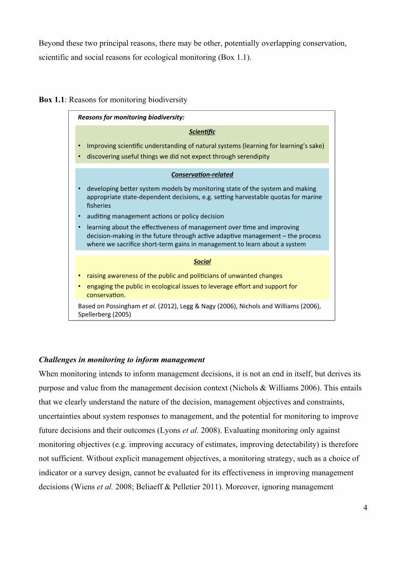
Beyond these two principal reasons, there may be other, potentially overlapping conservation,

scientific and social reasons for ecological monitoring (Box 1.1).

Box 1.1: Reasons for monitoring biodiversity

Challenges in monitoring to inform management

When monitoring intends to inform management decisions, it is not an end in itself, but derives its

purpose and value from the management decision context (Nichols & Williams 2006). This entails

that we clearly understand the nature of the decision, management objectives and constraints,

uncertainties about system responses to management, and the potential for monitoring to improve

future decisions and their outcomes (Lyons et al. 2008). Evaluating monitoring only against

monitoring objectives (e.g. improving accuracy of estimates, improving detectability) is therefore

not sufficient. Without explicit management objectives, a monitoring strategy, such as a choice of

indicator or a survey design, cannot be evaluated for its effectiveness in improving management

decisions (Wiens et al. 2008; Beliaeff & Pelletier 2011). Moreover, ignoring management

Scien&fic(!

•  Improving!scien.fic!understanding!of!natural!systems!(learning!for!learning’s!sake)!•  discovering!useful!things!we!did!not!expect!through!serendipity!

!Conserva&on/related(

!

•  developing!be?er!system!models!by!monitoring!state!of!the!system!and!making!appropriate!state@dependent!decisions,!e.g.!seCng!harvestable!quotas!for!marine!fisheries!

•  audi.ng!management!ac.ons!or!policy!decision!•  learning!about!the!effec.veness!of!management!over!.me!and!improving!

decision@making!in!the!future!through!ac.ve!adap.ve!management!–!the!process!where!we!sacrifice!short@term!gains!in!management!to!learn!about!a!system!

Social((

•  raising!awareness!of!the!public!and!poli.cians!of!unwanted!changes!•  engaging!the!public!in!ecological!issues!to!leverage!effort!and!support!for!

conserva.on.!!!Based!on!Possingham!et#al.#(2012),!Legg!&!Nagy!(2006),!Nichols!and!Williams!(2006),!

Spellerberg!(2005)!!!!

Reasons(for(monitoring(biodiversity:(

5

objectives for monitoring can lead to expensive and irreversible mistakes (Lindenmayer, Piggott &

Wintle 2013). For example, the extinctions of the Christmas Island pipistrelle (Pipistrellus murrayi)

in 2009 and Yangtze River dolphin (Lipotes vexillifer) in 2006 (Turvey et al. 2007; Beeton et al.

2010; Martin et al. 2012b; Zhang et al. 2015), in spite of ongoing monitoring efforts, suggest a lack

of understanding of how monitoring translates into relevant conservation actions (Lindenmayer,

Piggott & Wintle 2013). Many other species and ecosystems across the globe currently face

imminent local, regional, or global extinction (Butchart et al. 2005). Monitoring schemes that help

decision makers to respond quickly and decisively to biodiversity declines and their causes are

critical for threatened biodiversity (Martin et al. 2012b).

Although, we have seen repeated calls for monitoring to adequately inform policy and actions

(Nichols & Williams 2006; Mace & Baillie 2007; Collen & Nicholson 2014), a number of

challenges limit our ability to design and select effective monitoring strategies, especially when

managing multiple threats. Firstly, monitoring is often viewed as a stand-alone activity, and is

rarely evaluated for its benefit for management decision-making (Tulloch, Chadès & Possingham

2013). Moreover, the approaches to evaluate the extent to which alternative monitoring strategies

can change management decisions are currently limited (see Optimal monitoring section on page

10). Secondly, despite the limited funding and the pressure to spend resources in a transparent and

accountable manner, surprisingly few studies explicitly consider the cost of monitoring (but see

Mansson et al. 2011; Tulloch, Possingham & Wilson 2011), which can significantly increase the

rigor and transparency in decision-making (Baxter et al. 2006). Finally, management decisions are

usually confounded by uncertainty, complexity and incomplete information regarding species’

responses to natural variation, threats and management; and they depend on the costs and benefits

of management actions (Carwardine et al. 2009; Williams & Johnson 2013). Systematic approaches

to evaluate competing monitoring strategies that reduce uncertainty in the decision process and

improve management outcomes are limited (e.g. Field et al. 2004; Maxwell et al. 2015; Wilson,

Rhodes & Possingham 2015); and for managing multiple threats, approaches are lacking entirely.

Types of monitoring for management decision-making

A number of different types of biodiversity monitoring have been proposed in the literature

(Vaughan et al. 2001; Spellerberg 2005; e.g. Lindenmayer & Gibbons 2012). While we lack an

overarching typology for ecological monitoring, I identify four broad and overlapping categories of

monitoring for management decision-making: mandated monitoring, monitoring for public

6

relations, surveillance monitoring, and question-driven monitoring. My thesis focuses on question-

driven monitoring, particularly for the purpose of making targeted management decisions.

Mandated monitoring is used when environmental data are gathered as per government legislation,

political directive or international conventions (Lindenmayer & Likens 2010). These data generally

report on observed states or changes in an ecosystem, rather than identify the mechanisms

influencing the system. Mandated monitoring focuses on assessing compliance against pre-defined

standards or targets, e.g. monitoring to report on the progress towards the Aichi Targets of the

Convention on Biological Diversity (Leadley et al. 2014).

Monitoring for public relations aims to raise public awareness regarding environmental issues and

leverage their support for conservation. It is usually run by governmental or non-governmental

organisations and often engages the public for data collection or for disseminating the findings of an

investigation. For example, citizen science programs such as Bird Count India (www.birdcount.in)

and Canadian Nature Watch (www.naturewatch.ca) have encouraged members of the public to

participate in academic research.

Surveillance monitoring intends to provide ad hoc ecological insights, and is usually devoid of

specific questions or underlying study design (Lindenmayer & Likens 2010). It may be carried out

for the sake of curiosity, to generate new ideas, discover unforseen patterns and may even have

serendipitous impact on management decision-making and public policy (Wintle, Runge & Bekessy

2010). However, its role in informing management decisions is unclear (Wintle, Runge & Bekessy

2010; Lindenmayer, Piggott & Wintle 2013). Examples include data typically collected over a long

time frame and wide geographic regions such as the North American Breeding Bird Survey and the

Continuous Plankton Recorder (Richardson et al. 2006; Sauer et al. 2013).

Question-driven monitoring, involves monitoring to test a-priori hypotheses, or to discern between

competing hypotheses that may be related to scientific queries or targeted management decisions

(Lindenmayer & Likens 2010). Such a targeted monitoring approach typically links the information

obtained from monitoring to the question being addressed. For example, monitoring within the U.S.

Fish and Wildlife Services Adaptive Harvest Management Program for waterfowl is specifically

aimed at predicting the consequences of regulating duck hunting regulations and specifying

guidelines within which States can set their hunting seasons. (U.S. Fish and Wildlife Service 2015).

7

Each of the above types of monitoring can use direct or indirect measurements of a targeted entity,

or subset of entities, of conservation interest in response to environmental conditions or

management interventions (Lindenmayer & Likens 2011). To illustrate this distinction, consider a

threatened freshwater system where the management objective is to improve invertebrate

biodiversity in a stream by managing effluent discharge. A manager may measure the abundance or

diversity of freshwater invertebrates in the stream directly to assess its response to the threat. This

type of approach to tackle environmental problems focuses efforts on direct measures that target the

management objective specifically (e.g., using the above example, attempting to sample the

complete biodiversity of the system of interest). Alternatively, the manager may measure indicators

which represent a subset of the specific management objectives (e.g., presence/absence of

particularly sensitive or representative members of the stream community) or measures which are

attributes of the system that might be more easily measured than fundamental management targets

themselves (e.g. pollutant concentrations in the stream) but are believe to be strongly correlated

with the stated objectives. This approach presumes that the entities targeted for measurement are

proxies of other ecological elements, processes, or properties that are too difficult to measure

directly, due to logistical, financial, or technological reasons (Landres, Verner & Thomas 1988;

Fleishman & Murphy 2009). Although indicators are not direct measures of the management

objective, they are often partial, direct measures of objectives or indirect measure that are related to

the management objectives under the assumption of correlation.

Indicators are used in various aspects of conservation science and management, including

identifying areas of conservation significance, measuring and communicating the effects of natural

or anthropogenic processes on biological systems, and helping advocate for conservation issues

(Caro 2010). Often, they are used to learn about the impacts of threats such as atmospheric

pollution, habitat modification, fisheries or logging impacts or climate change on an ecosystem (e.g.

Ravera 2001; Gjerdrum et al. 2003; Kennard et al. 2005; Filgueiras et al. 2015). For example,

species such as the northern spotted owl which is used as an indicator of old-growth logging in

Pacific Northwest, USA (Doak 1989), landscape indicators such as patch shape and edge to

represent extent of habitat fragmentation (Lindenmayer et al. 2002), and atmospheric sulphur or

nitrogen deposition as an indicator of soil acidification (Heink & Kowarik 2010a). However, it

could be argued that monitoring of spotted owls is a direct measure of the effects of old-growth

forest loss on this species (i.e., the conservation of this species is a management objective in itself,

8

possibly along with other complementary and competing objectives such as maintaining forests and

providing extractive economic benefits). Thus, from one perspective or decision context, owls may

be an indicator of forest loss but, from another, a direct measure of a conservation objective. It

could also be argued that patch shape and edge have been selected as the best direct way to measure

a difficult concept like habitat fragmentation. Fragmentation itself is often a ‘means’ objective to

some other, more fundamental management goal of habitat itself or the system/organisms such

habitat supports (Failing & Gregory 2003). In this context, patch shape/edge could actually be

considered as an indicator for the true underlying management objective. While the efficacy of

indicators in conservation has drawn mixed reviews (Carignan & Villard 2002; Seddon & Leech

2008; Fleishman & Murphy 2009), their practical utility has made their use almost standard

monitoring practice in ecological systems (Caro 2010; Siddig et al. 2016).

Decision-making for monitoring

Many scientific articles and books outline the principles of good monitoring, covering aspects from

design and field methods to project management (e.g. Legg & Nagy 2006; Lindenmayer et al.

2012). A number of these aim to increase the efficiency of monitoring, for example by accounting

for species detectability (Pollock et al. 2002; Kéry & Schmidt 2008), allocating optimal monitoring

effort (Field, Tyre & Possingham 2005; Rhodes & Jonzén 2011) or improving the statistical power

of monitoring to enable informed decision-making (Field et al. 2004; Rhodes et al. 2006).

Numerous criteria, methods and frameworks have been proposed for selecting and evaluating

indicators (e.g. Carignan & Villard 2002; Gregory et al. 2005; Niemeijer & de Groot 2008; Heink

& Kowarik 2010b; Beliaeff & Pelletier 2011). However, it appears that most studies on monitoring

design and indicator selection focus on improving monitoring strategies with respect to the

monitoring objective (e.g. sensitivity to detect change, surrogacy) rather than improving the

efficacy of monitoring to inform management decisions (but see, e.g. Tulloch, Possingham &

Wilson 2011; Lindenmayer, Barton & Pierson 2015). Approaches such as structured decision-

making and decision theory provide ways to design, implement and evaluate management choices

(Raiffa & Schlaifer 1961; Gregory 2012), and are also relevant for evaluating monitoring choices

for management. Most importantly, these approaches help frame monitoring choices as part of the

decision making process, thereby establishing a clear link between monitoring and management.

9

Decision theory

Decision-theory provides a rational procedure for discriminating between alternative decisions or

actions, when the outcomes of these decisions are uncertain (Raiffa & Schlaifer 1961; North 1968).

It does so by clearly specifying (1) the management objective; (2) the alternative management

actions; (3) a model of the system (state and dynamics); (4) constraints that bind the decision, e.g.

budgets; and (5) uncertainty in the model and its parameters (Shea & NCEAS Working Group on

Population Management 1998). After specifying the context of the decision problem, decision

analysis employs a decision-making protocol and/or mathematical or qualitative tools for evaluating

the consequences of management alternatives to find the best solution (Possingham et al. 2001).

Monitoring decisions present similar problems to those outlined for management decision-making

and require a clear understanding of the management objective, competing monitoring strategies

(i.e. actions) and the associated costs while accounting of variation in perceived management

outcomes based on information obtained from monitoring (i.e., partial observability). Using

decision theory, we can compare different monitoring strategies based on their risks and benefits

(Edwards 1954; Raiffa 1968; Hastie & Dawes 2001; Polasky et al. 2011).

Structured decision-making

Structured decision-making (SDM) is a systematic and collaborative approach to identifying and

evaluating creative solutions to complex decision problems, e.g. multiple objective decisions

problems in environmental management and public policy involving multiple stakeholders

(Gregory 2012). The conservation literature has seen the application of the SDM approach towards

various biodiversity management objectives, such as recovery planning for endangered species

(Gregory & Long 2009), optimally allocating resources among alternative management strategies

under uncertainty regarding the ecosystem as well as the the effectiveness of management

alternatives (Moore & Runge 2012) or establishing thresholds for conservation planning (Addison,

de Bie & Rumpff 2015, Martin et al. 2009). These studies and other studies using SDM from the

conservation as well as the business literature show how SDM embodies an overarching framework

that can use a diverse set of tools for making and analysing decisions (Lyons et al. 2008). The

advantage of using SDM is that it explicitly considers all alternatives at each step of the process

(Figure 1.1) rather than prescribing a preferred solution (Gregory 2012), making it a valuable

approach for guiding decisions for management. Therefore, it offers a way to implement a decision-

making process systematically while ensuring that the choices are well informed.

10

The general approach involves decomposing a decision into basic elements (objectives, actions and

outcomes), developing these elements collaboratively with other stakeholders, and then finding the

solution by using decision-analytic tools (Lyons et al. 2008). The first step in the SDM involves

clarifying the decision context (Gregory 2012). This involves defining what decision is being made

and why. Key stakeholders involved in the decision process are identified (e.g. ultimate decision

maker, technical experts, landholders) are their roles and responsibilities are established.

Constraints that bind the decision are also identified, e.g. legal or financial constraints. SDM

requires a clear statement of objectives. These help explicitly state the intentions of the decision

process i.e. specific outcomes or performance measures that guide the decision-making process and

are used to evaluate the success of actions (Clemen 1996). Generally, they can be expressed in

terms of maximizing (or minimizing) one or more quantitative measures of performance. Failing &

Gregory 2003 emphasize the imporance of differentiating fundamental and means objectives for

decision-making: the former being the results decision-makers care about most and the latter are the

steps that are needed to help accomplish fundamental objectives (Lyons 2008). Alternatives are a

set of actions that together provide a comprehensive approach to solving the decision problem

(Gregory 2012). Listing the potential actions is not easy because effective actions may not exist or

may be unacceptable to some stakeholders (Lyons 2008). A number of considerations need to be

accounted for when developing a list of alternative actions such as technical feasibility, public

acceptability or legal and regulatory constraints on them (Lyons 2008, Gregory 2012). Thus,

articulating a set of alternative actions requires scientific and stakeholder input while considering

the potential efficacy and political support for the suggested actions (Lyons 2008). The next step in

SDM is to estimate consequences of the alternatives in terms of the objectives and evaluation

criteria (Gregory 2012). This usually involves a model to describe how we think the system

responds to management actions such as decision trees, Bayesian networks, influence diagrams.

This is an analytical step usually performed by technical experts with input from stakeholders

(Gregory 2012). There are numerous techniques for analysis, with the appropriate method

depending on the nature of the decision, the form of the objectives, and the capability of the model

(Lyons 2008). Uncertainty plays an important role in any decision process. Evaluating the

performance of competing actions also requires that uncertainty be incorporated in decision-

making, for example through the use of sensitivity analysis, scenario analysis, etc. However, it is

important to understand that though there will be many uncertainties, the idea here is to identify

those sources of uncertainty that play a central role in the dynamics of the decision (Gregory 2012).

In doing so, SDM can highlight the trade-offs between alternatives so that stakeholders can make

11

value-based choices. Here, the decision maker and other stakeholders make an informed decision by

being explicit of the choices they make, and demonstrating an understanding of the decision scope

and context, evaluation criteria, uncertainties and trade-offs. Finally, the decision is implemented

and the outcome of the decision (if possible) can be monitored and assessed to ensure things are

unfolding as expected and to understand which uncertainties can be resolved (Gregory 2012).

Figure 1.1: Steps in structured decision-making. Source: Gregory (2012)

Adaptive management

Much like SDM, the process of adaptive management (AM) involves objective-driven decision

making through time. Adaptive management is a special case of structured decision-making;

applicable when the decision recurs over time or space, and there is uncertainty about how the

system operates (Lyons et al. 2008). Here, management actions at a given decision point are

informed by what is known (and not known) at that time (Williams 2011, Walters 1990, Holling

1978). Comparing the observed against the predicted responses or consequences helps update our

understanding of system behaviour, and therefore facilitates learning in this process. Monitoring

within AM provides the feedback loop to complete the cycle of planning, implementation, and

evaluation. By integrating learning through monitoring into decision-making, AM allows decision-

12

makers to achieve management objectives while also generating new knowledge about system

response to management.

Adaptive management approaches can be classified as passive or active (Williams 2011; Hauser &

Possingham 2008; Williams, Nichols & Conroy 2002) although there appears to be considerable

ambiguity in the use of these terms. Integrating the ability to improve our understanding of the

system (through continual monitoring and evaluation) and reduce uncertainty is an essential part of

the adaptive decision-making process (Williams 2011). The way uncertainty is uncertainty is

recognized and treated is the key difference between the two AM approaches. Active AM is widely

agreed to be the management strategy that explicitly incorporates learning; it pursues the reduction

of uncertainty through management interventions. Passive AM focuses on maximising returns by

focussing on the resource objectives and learning is a useful but unintended by-product of decision-

making (Walters, 1990). In active AM, the knowledge or belief state of competing hypotheses (i.e.,

weights on competing models) is treated as a model variable in the optimization; the evolution of

these weights are accounted for over time, allowing for an expectation of learning and the ability to

select actions that improve long-term learning over short-term benefits (i.e., a recommendation of

probing actions). Passive AM, on the other hand, produces an optimal decision policy under the

assumption that the belief state (weights) is static over the management time horizon and, thus,

learning is not accounted for in future decisions. Monitoring provides the learning outside of the

optimization, requiring a new policy to be optimized after each observation provides a means to

update the belief state.

Several sources of uncertainty can influence or impede effective management decisions, such as

measurement error, natural environmental variation, and model or structural uncertainty (Regan,

Colyvan & Burgman 2002; Lyons et al. 2008). AM is designed principally to addresses structural

uncertainty. The other sources of uncertainty are, of course, considered in the general decision

analytic approach (e.g., SDM), but the specific role of AM is to focus monitoring on reducible

uncertainty as opposed to what is usually thought of as irreducible forms (e.g., environmental

stochasticity). Therefore, AM prescribes management actions that evolve as uncertainty is reduced

through time.

13

Both structured decision-making and adaptive management frequently rely on the use of decision-

analytic tools such as multi-criteria decision analysis and optimisation to evaluate alternate

management actions with uncertain outcomes (Edwards, Miles & Von Winterfeldt 2007).

Optimal monitoring

Research in optimal monitoring utilises principles of decision theory, SDM and AM to link

monitoring and management activities for effective decision-making. Examples include questions

on whether and when to monitor (Chadès et al. 2008; McDonald-Madden et al. 2010a), how often

to monitor (Hauser, Pople & Possingham 2006), and how to target monitoring to resolve key

uncertainties (Runge, Converse & Lyons 2011; Maxwell et al. 2015). These approaches look for

optimal monitoring solutions under clearly stated management objectives and their associated

constraints, such as a monitoring budget, alternative monitoring strategies, and the uncertainty

regarding system response to management actions.

Monitoring to inform management of multiple threats

Nearly all ecological systems face multiple threats (e.g. Vorosmarty et al. 2010; Evans et al. 2011)

that together play a significant role in driving ecosystem changes and biodiversity declines (Brook,

Sodhi & Bradshaw 2008; Crain, Kroeker & Halpern 2008; Mantyka-Pringle, Martin & Rhodes

2012). For example, coral reefs face multiple pressures from coastal development, pollution,

overfishing, destructive fishing practices and rises in sea temperature and sea level due to climatic

shifts (Hughes, Huang & Young 2013; Auerbach, Tulloch & Possingham 2014). Terrestrial

vertebrates in the north-west of Australia are threatened by fire, invasive species and grazing

pressures (Carwardine et al. 2012). To manage multiple threats effectively, we need reliable

information on their relative impacts to biodiversity and the consequences of different threat

reduction activities, but these are often uncertain (Evans, Possingham & Wilson 2011; Auerbach,

Tulloch & Possingham 2014).

Monitoring plays an important role in reducing uncertainty regarding the status of threats and when

interventions are needed. However, this is not easy when multiple threats operate, as it may

confound our ability to separate the effect of each threat on target biodiversity (Breitburg et al.

1998). For example, in the Pilbara region in northwestern Australia, threats such as over-grazing,

invasive species, altered fire regimes, altered hydrological regimes and extractive mining have

varying degrees of impact on different species in the ecosystem (McKenzie, van Leeuwen & Pinder

14

2009; Carwardine et al. 2014). Some threats such as altered fire regimes result in declines in most

species, e.g. the western brushtail possum (Trichosurus vulpecula) and the southern brown

bandicoot (Isoodon obesulus), but benefit others like the tammar wallaby (Macropus eugenii)

because it increases grass growth and fruiting of small bushes following fires (Christensen 1980). In

such a multi-species, multi-threat system, managers need to not only tease apart species responses

to different threats and their corresponding management actions, but also understand the influence

of uncertainty on subsequent monitoring and management decisions.

Research has primarily focused on identifying indicators to learn about individual threats (e.g.

Tulloch, Possingham & Wilson 2011) and to estimate the cumulative effect of multiple threats, i.e.

the chronic exposure over time to several stressors, based on data from published studies (Brook,

Sodhi & Bradshaw 2008; Crain, Kroeker & Halpern 2008; Mantyka-Pringle, Martin & Rhodes

2012). Our understanding of what to monitor to learn about the impacts of multiple threats on

species, and how to make these decisions in complex real-word conservation problems, is therefore

limited. To address this limitation, we need to develop decision-analytic approaches to evaluate

alternative monitoring choices for informed management decision in multi-species, multi-threat

systems.

Decision tools for monitoring multiple threats

The literature offers a number of tools to aid decision-making, such as decision trees, control charts,

Bayesian networks, Markov models, pareto-analysis, and decision matrices (Burgman 2005;

Ramsey & Veltman 2005; Marcot et al. 2006; Johnson et al. 2011; Addison et al. 2013; Neil &

Fenton 2013). Two approaches of particular value for analysing monitoring decision problems are

value of information and cost-effectiveness analyses.

Value of information (VOI) analysis can explicitly indicate the optimal management decision that

arises from new information, as obtained through monitoring or research, versus existing

information (Raiffa & Schlaifer 1961; North 1968; Runge, Converse & Lyons 2011). It evaluates

the benefit of collecting additional information for management decision making to reduce

uncertainties before making a decision. The most important uncertainties are those that have the

highest chance of resulting in a change to a more effective strategy (Runting, Wilson & Rhodes

2013; Maxwell et al. 2015). VOI is widely used in economic evaluations of health care and risk

management (Claxton et al. 2004; Yokota & Thompson 2004); fisheries management (Mäntyniemi

15

et al. 2009); risk assessment for climate change mitigations (Kousky & Cooke 2012) and

environment insurance schemes (Laxminarayan & Macauley 2012). VOI has seen recent uptake in

the conservation literature (Runge, Converse & Lyons 2011; Sahlin et al. 2011; Moore & Runge

2012; Maxwell et al. 2015), but has rarely been applied to evaluating monitoring choices for

management (see Pannell & Glenn 2000).

Decision-making for monitoring to inform management typically includes an explicit management

decision context, uncertainties in multiple parts of the decision process, and multiple ways of

reducing uncertainty, or choosing an element of a system for which to reduce uncertainty. VOI

analysis is therefore particularly applicable to monitoring decisions. Unlike other decision-making

approaches, VOI explicitly links the effort (or resources) directed at reducing uncertainty to the

improvement of outcomes from management decisions. Although researchers are attempting to

make VOI more user-friendly through the use of excel worksheets or multivariate analysis (Runge,

Converse & Lyons 2011; see Canessa et al. 2015), the calculations are technically challenging and

managers may not be familiar with decision-theoretic principles and notation (Canessa et al. 2015).

Cost effectiveness analysis (CE analysis) is an economic analysis to examine the relative outcomes

and costs of different means of accomplishing an objective, to select the one with the highest

effectiveness relative to its cost. CE analysis is useful for conservation prioritisation because it can

explicitly incorporate financial considerations while avoiding the ethical and practical dilemmas

associated with putting a monetary value on species or ecosystems (Laycock et al. 2009). For

example, CE analysis has been used to prioritise threatened species recovery projects (Cullen,

Moran & Hughey 2005; Joseph, Maloney & Possingham 2008; Briggs 2009; Laycock et al. 2009),

actions to mitigate threats to biodiversity (Carwardine et al. 2012), and landscape-scale

environmental projects (Pannell et al. 2012). A related concept is the return on investment analysis,

which measures the increase in the outcomes per unit cost of an action (Murdoch et al. 2007;

Possingham et al. 2012). These approaches have seen limited uptake for monitoring decision-

making, but can be extremely useful because they are straightforward and address resource

allocation problems common to biodiversity-monitoring decisions. Therefore, together they can

help to most effectively allocate limited resources to monitoring while generating the biggest

returns for management.

16

Thesis aims and overview

In this thesis, I examine structured frameworks for monitoring and indicator selection, and provide

a better understanding of the challenges of monitoring to inform complex, real-world conservation

decisions. The approaches and tools I develop focus on multi-species, multi-threat decision

problems, and help evaluate monitoring choices based on their costs and benefits. I also apply the

proposed approaches to case study scenarios of decision-making that vary in context and scale.

My research has four specific objectives:

1. To determine whether approaches for choosing indicator species for management explicitly

consider management outcomes in a structured way.

2. To evaluate the benefit of monitoring species (i.e. with and without experimental

manipulation of threats) for managing multiple threats for multiple species.

3. To evaluate how uncertainty regarding the effectiveness of threat management actions

influences optimal monitoring and management decisions for multiple threats.

4. To develop a simple tool based on a return on investment framework to make monitoring

decisions in multi-species, multi-threat systems.

This thesis consists of six chapters: an Introduction (this chapter), followed by four analytical

chapters and a synthesis chapter (Figure 1.2).

In chapter two, I systematically review the literature to investigate two questions. First, whether

monitoring strategies for management of biodiversity - particularly the use of indicator species, are

selected under clearly defined management objectives. Second, whether the approaches used for

selecting indicator species account for monitoring and management objectives, constraints, actions,

uncertainty and outcomes of alternate indicator choices. In this review, I identify the gaps that lay

the foundation for the following three chapters of the thesis, which introduce new decision-analytic

approaches and insights for choosing monitoring strategies for the management of multi-species,

multi-threat systems.

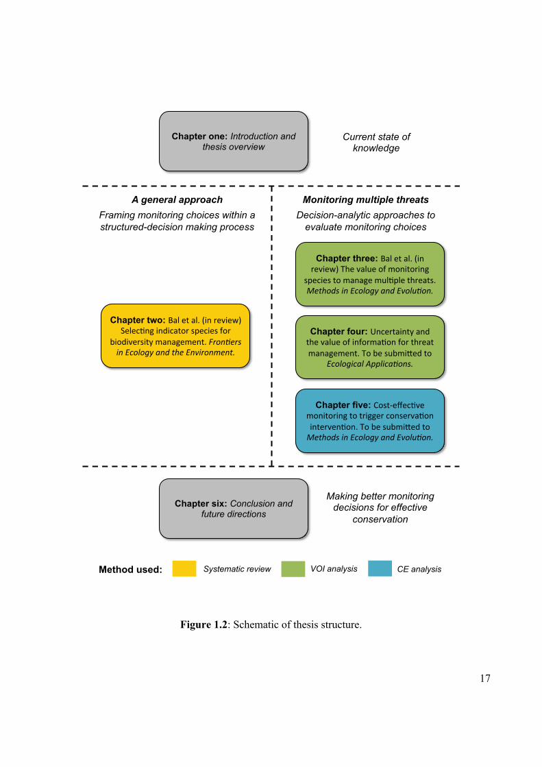
17

Figure 1.2: Schematic of thesis structure.

Chapter one: Introduction and thesis overview

Chapter two: Bal$et$al.$(in$review)$Selec1ng$indicator$species$for$

biodiversity$management.$Fron%ers(in(Ecology(and(the(Environment.(((((

Chapter three: Bal$et$al.$(in$review)$The$value$of$monitoring$

species$to$manage$mul1ple$threats.$Methods(in(Ecology(and(Evolu%on.$

Chapter four: Uncertainty$and$the$value$of$informa1on$for$threat$management.$To$be$submi?ed$to$$

Ecological(Applica%ons.(

Chapter five: CostAeffec1ve$monitoring$to$trigger$conserva1on$interven1on.$To$be$submi?ed$to$$Methods(in(Ecology(and(Evolu%on.(

Chapter six: Conclusion and future directions

A general approach

Framing monitoring choices within a structured-decision making process

Monitoring multiple threats

Decision-analytic approaches to evaluate monitoring choices

Making better monitoring decisions for effective

conservation

Current state of knowledge

Systematic review CE analysis VOI analysis Method used:

18

In chapter three, I demonstrate the use of VOI analysis to examine whether monitoring of species

(subjected to multiple threats) improves our ability to inform management of multiple threats for

multiple species. Specifically, I compare the effectiveness of different monitoring approaches to

learn about the threats i.e. monitoring just species and monitoring with experimentation. The latter

type of monitoring considers manipulating the system in order to better to learn about the threats

(e.g. controlling predator abundance or the degree of disturbance). This study proposes simple

principles for understanding when monitoring species is likely to be valuable in guiding threat

management. This is the first study to utilise the VOI approach to identify monitoring strategies that

inform decisions about threat management for multiple threats and multiple species.

In chapter four, I use the VOI approach to examine how uncertainty regarding the effectiveness of

threat management actions influences optimal monitoring and management decisions. The approach

presented here allows us to address conservation decisions informed by the magnitude of

management effectiveness, which was not considered in chapter three. Specifically, I quantify how

the value of monitoring to inform the management of multiple threats is influenced by two factors:

(1) the differences in prior knowledge regarding the benefit of management for a given threat and

(2) the uncertainty regarding the effectiveness of alternative management actions. I also explore

rules regarding how managers can choose the best monitoring strategy for effective threat

management under uncertainty in multi-threat systems.

In chapter five, I develop a CE analysis framework to estimate the return on investment of

selecting indicators of threats in multi-species, multi-threat systems. This study proposes a simple

tool for real-world conservation decision-making that evaluates the cost-effectiveness of alternative

indicators using six key factors including monitoring efficiency, management outcomes and

economic constraints for decision-making. The proposed framework is applicable to a large number

of species, threats and indicators. This is the first study to utilise the return on investment

framework to compare indicators for monitoring threats and triggering management interventions.

Chapter six – Discussion synthesises the previous chapters and discusses the implications of these

studies for developing effective monitoring strategies for management. Limitations and future

research priorities are also discussed in this chapter.

19

Selecting indicator species for

biodiversity management

Under review in Frontiers in Ecology and Environment

20

Chapter two – Selecting indicator species for biodiversity management

Abstract

Indicator species are frequently proposed to inform biodiversity management, but whether they are

selected under clear management objectives or evaluated for their ability to improve decisions

remains unclear. We review the scientific literature to assess if methods used to select indicator

species account for key monitoring and management decision factors such as objectives and their

constraints, actions, uncertainties and biodiversity outcomes. We find that most indicator selection

studies focus on improving the monitoring efficiency rather than the management effectiveness,

potentially leading to ineffective indicators. Only 21% of studies explicitly accounted for the

management objectives and actions. More worryingly, 94% of studies and half of all indicator

selection methods overlook constraints when setting objectives (e.g. budget) and uncertainties (e.g.

in detection or management effectiveness). To improve indicator selection for management

decision-making, we recommend clearly defining the management context for monitoring,

developing practical methods focused on improving management outcomes, and incorporating

uncertainty into the selection process.

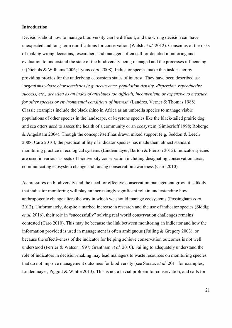
21

Introduction

Decisions about how to manage biodiversity can be difficult, and the wrong decision can have

unexpected and long-term ramifications for conservation (Walsh et al. 2012). Conscious of the risks

of making wrong decisions, researchers and managers often call for detailed monitoring and

evaluation to understand the state of the biodiversity being managed and the processes influencing

it (Nichols & Williams 2006; Lyons et al. 2008). Indicator species make this task easier by

providing proxies for the underlying ecosystem states of interest. They have been described as:

‘organisms whose characteristics (e.g. occurrence, population density, dispersion, reproductive

success, etc.) are used as an index of attributes too difficult, inconvenient, or expensive to measure

for other species or environmental conditions of interest’ (Landres, Verner & Thomas 1988).

Classic examples include the black rhino in Africa as an umbrella species to manage viable

populations of other species in the landscape, or keystone species like the black-tailed prairie dog

and sea otters used to assess the health of a community or an ecosystem (Simberloff 1998; Roberge

& Angelstam 2004). Though the concept itself has drawn mixed support (e.g. Seddon & Leech

2008; Caro 2010), the practical utility of indicator species has made them almost standard

monitoring practice in ecological systems (Lindenmayer, Barton & Pierson 2015). Indicator species

are used in various aspects of biodiversity conservation including designating conservation areas,

communicating ecosystem change and raising conservation awareness (Caro 2010).

As pressures on biodiversity and the need for effective conservation management grow, it is likely

that indicator monitoring will play an increasingly significant role in understanding how

anthropogenic change alters the way in which we should manage ecosystems (Possingham et al.

2012). Unfortunately, despite a marked increase in research and the use of indicator species (Siddig

et al. 2016), their role in “successfully” solving real world conservation challenges remains

contested (Caro 2010). This may be because the link between monitoring an indicator and how the

information provided is used in management is often ambiguous (Failing & Gregory 2003), or

because the effectiveness of the indicator for helping achieve conservation outcomes is not well

understood (Ferrier & Watson 1997; Grantham et al. 2010). Failing to adequately understand the

role of indicators in decision-making may lead managers to waste resources on monitoring species

that do not improve management outcomes for biodiversity (see Saraux et al. 2011 for examples;

Lindenmayer, Piggott & Wintle 2013). This is not a trivial problem for conservation, and calls for

22

solutions to improve the links between indicator selection and management outcomes as well as an

appraisal of current indicator selection practices.

If the purpose of monitoring is to inform management decisions, indicator selection must clearly

specify the decision context, including the nature of the decision, management objectives,

uncertainties about system response to management, and the potential for monitoring to improve

future decisions and their outcomes (Lyons et al. 2008). Without explicit management objectives,

an indicator cannot be evaluated for its effectiveness in guiding management (Wiens et al. 2008;

Beliaeff & Pelletier 2011) and therefore cannot logically inform decision-making (Lyons et al.

2008). Other factors such as cost or feasibility of monitoring also influence indicator selection

(Tulloch, Possingham & Wilson 2011) along with ecological factors such the nature of the

ecological system (Wiens et al. 2008), and must be considered to avoid choosing indicators that are

too expensive to monitor or those that are not responsive to threats in the system. We therefore need

to account for all such decision-making factors when choosing the appropriate indicator(s) for

management.

Structured decision-making (SDM; Gregory 2012) and adaptive management (Holling 1978;

Walters & Holling 1990) offer logical ways of making informed decisions. SDM is a systematic

and collaborative approach to identifying and evaluating creative solutions to complex decision

problems by engaging stakeholders, experts and decision makers in productive decision-oriented

analysis (Gregory 2012). Adaptive management is an iterative process of decision-making that can

help identify and sequentially resolve critical uncertainties in the decision process to improve

decisions over time (Holling 1978). These approaches often solve different problems, but both

frequently rely on the use of decision-analytic tools such as multi-criteria decision analysis and

optimisation to evaluate alternate management actions with uncertain outcomes (Edwards, Miles &

Von Winterfeldt 2007). Research in optimal monitoring uses SDM and adaptive management to

link monitoring and management activities for effective decision-making. Examples include

questions on whether and when to monitor (Chadès et al. 2008; McDonald-Madden et al. 2010a),

how often to monitor (Hauser, Pople & Possingham 2006), and how to target monitoring to resolve

key uncertainties in ecosystem processes or in management effectiveness (Runge, Converse &

Lyons 2011; Maxwell et al. 2015). These studies look for optimal monitoring solutions under

clearly stated management objectives and their associated constraints such as monitoring costs,

alternative monitoring actions such as competing indicator species, and uncertainty in the different

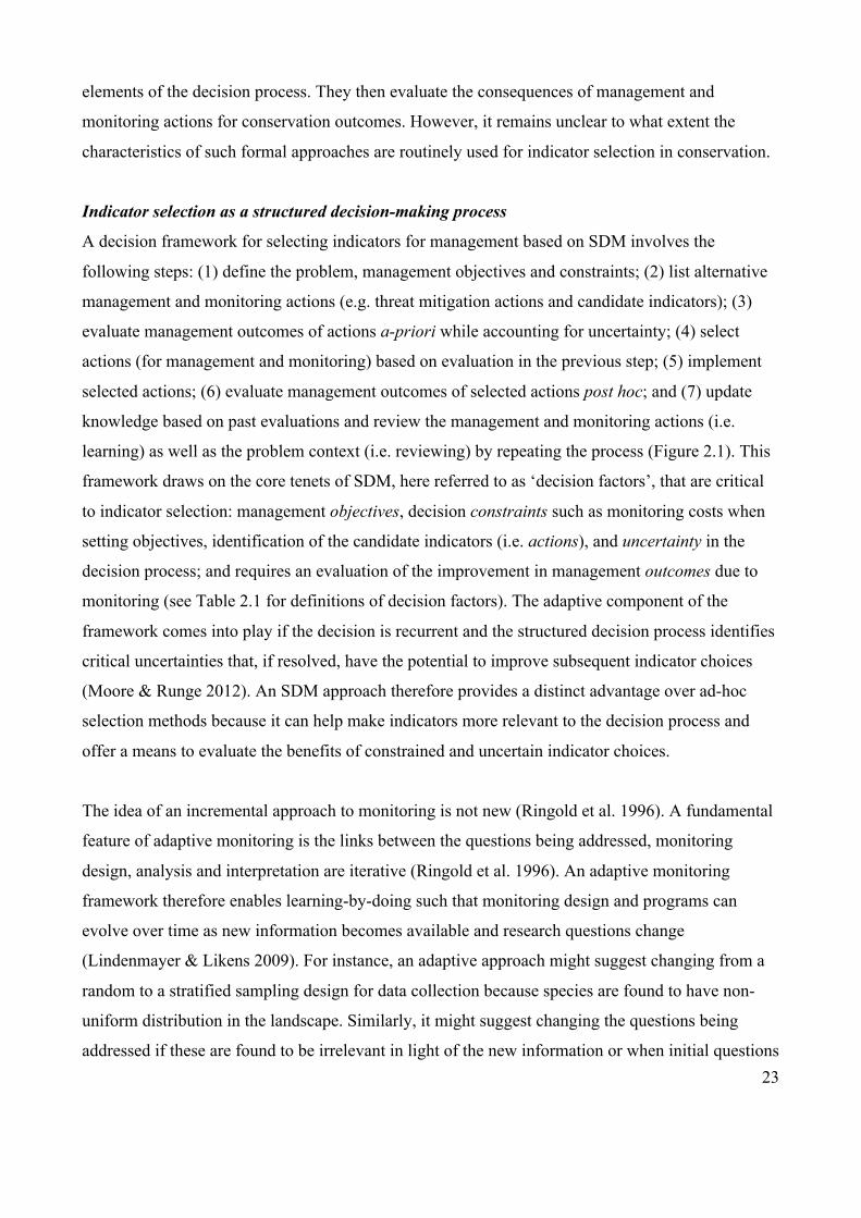
23

elements of the decision process. They then evaluate the consequences of management and

monitoring actions for conservation outcomes. However, it remains unclear to what extent the

characteristics of such formal approaches are routinely used for indicator selection in conservation.

Indicator selection as a structured decision-making process

A decision framework for selecting indicators for management based on SDM involves the

following steps: (1) define the problem, management objectives and constraints; (2) list alternative

management and monitoring actions (e.g. threat mitigation actions and candidate indicators); (3)

evaluate management outcomes of actions a-priori while accounting for uncertainty; (4) select

actions (for management and monitoring) based on evaluation in the previous step; (5) implement

selected actions; (6) evaluate management outcomes of selected actions post hoc; and (7) update

knowledge based on past evaluations and review the management and monitoring actions (i.e.

learning) as well as the problem context (i.e. reviewing) by repeating the process (Figure 2.1). This

framework draws on the core tenets of SDM, here referred to as ‘decision factors’, that are critical

to indicator selection: management objectives, decision constraints such as monitoring costs when

setting objectives, identification of the candidate indicators (i.e. actions), and uncertainty in the

decision process; and requires an evaluation of the improvement in management outcomes due to

monitoring (see Table 2.1 for definitions of decision factors). The adaptive component of the

framework comes into play if the decision is recurrent and the structured decision process identifies

critical uncertainties that, if resolved, have the potential to improve subsequent indicator choices

(Moore & Runge 2012). An SDM approach therefore provides a distinct advantage over ad-hoc

selection methods because it can help make indicators more relevant to the decision process and

offer a means to evaluate the benefits of constrained and uncertain indicator choices.

The idea of an incremental approach to monitoring is not new (Ringold et al. 1996). A fundamental

feature of adaptive monitoring is the links between the questions being addressed, monitoring

design, analysis and interpretation are iterative (Ringold et al. 1996). An adaptive monitoring

framework therefore enables learning-by-doing such that monitoring design and programs can

evolve over time as new information becomes available and research questions change

(Lindenmayer & Likens 2009). For instance, an adaptive approach might suggest changing from a

random to a stratified sampling design for data collection because species are found to have non-

uniform distribution in the landscape. Similarly, it might suggest changing the questions being

addressed if these are found to be irrelevant in light of the new information or when initial questions

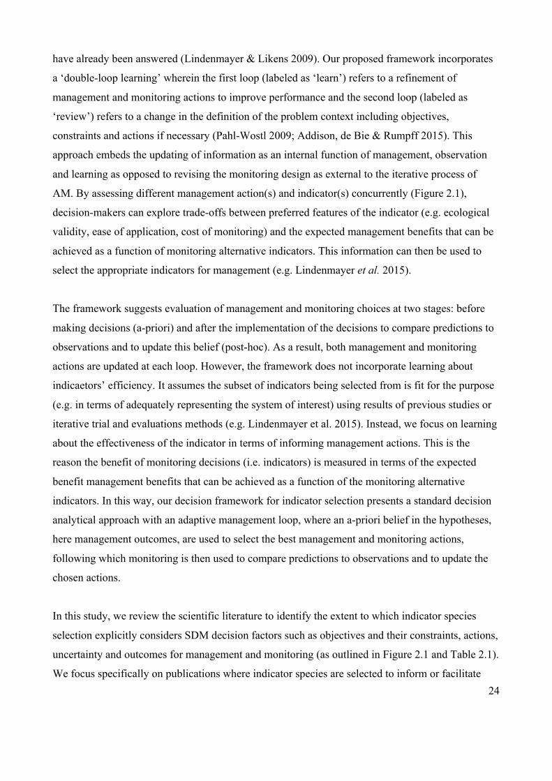
24

have already been answered (Lindenmayer & Likens 2009). Our proposed framework incorporates

a ‘double-loop learning’ wherein the first loop (labeled as ‘learn’) refers to a refinement of

management and monitoring actions to improve performance and the second loop (labeled as

‘review’) refers to a change in the definition of the problem context including objectives,

constraints and actions if necessary (Pahl-Wostl 2009; Addison, de Bie & Rumpff 2015). This

approach embeds the updating of information as an internal function of management, observation

and learning as opposed to revising the monitoring design as external to the iterative process of

AM. By assessing different management action(s) and indicator(s) concurrently (Figure 2.1),

decision-makers can explore trade-offs between preferred features of the indicator (e.g. ecological

validity, ease of application, cost of monitoring) and the expected management benefits that can be

achieved as a function of monitoring alternative indicators. This information can then be used to

select the appropriate indicators for management (e.g. Lindenmayer et al. 2015).

The framework suggests evaluation of management and monitoring choices at two stages: before

making decisions (a-priori) and after the implementation of the decisions to compare predictions to

observations and to update this belief (post-hoc). As a result, both management and monitoring

actions are updated at each loop. However, the framework does not incorporate learning about

indicaetors’ efficiency. It assumes the subset of indicators being selected from is fit for the purpose

(e.g. in terms of adequately representing the system of interest) using results of previous studies or

iterative trial and evaluations methods (e.g. Lindenmayer et al. 2015). Instead, we focus on learning

about the effectiveness of the indicator in terms of informing management actions. This is the

reason the benefit of monitoring decisions (i.e. indicators) is measured in terms of the expected

benefit management benefits that can be achieved as a function of the monitoring alternative

indicators. In this way, our decision framework for indicator selection presents a standard decision

analytical approach with an adaptive management loop, where an a-priori belief in the hypotheses,

here management outcomes, are used to select the best management and monitoring actions,

following which monitoring is then used to compare predictions to observations and to update the

chosen actions.

In this study, we review the scientific literature to identify the extent to which indicator species

selection explicitly considers SDM decision factors such as objectives and their constraints, actions,

uncertainty and outcomes for management and monitoring (as outlined in Figure 2.1 and Table 2.1).

We focus specifically on publications where indicator species are selected to inform or facilitate

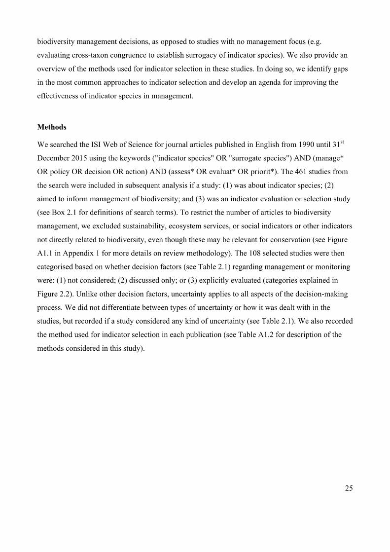
25

biodiversity management decisions, as opposed to studies with no management focus (e.g.

evaluating cross-taxon congruence to establish surrogacy of indicator species). We also provide an

overview of the methods used for indicator selection in these studies. In doing so, we identify gaps

in the most common approaches to indicator selection and develop an agenda for improving the

effectiveness of indicator species in management.

Methods

We searched the ISI Web of Science for journal articles published in English from 1990 until 31st

December 2015 using the keywords ("indicator species" OR "surrogate species") AND (manage*

OR policy OR decision OR action) AND (assess* OR evaluat* OR priorit*). The 461 studies from

the search were included in subsequent analysis if a study: (1) was about indicator species; (2)

aimed to inform management of biodiversity; and (3) was an indicator evaluation or selection study

(see Box 2.1 for definitions of search terms). To restrict the number of articles to biodiversity

management, we excluded sustainability, ecosystem services, or social indicators or other indicators

not directly related to biodiversity, even though these may be relevant for conservation (see Figure

A1.1 in Appendix 1 for more details on review methodology). The 108 selected studies were then

categorised based on whether decision factors (see Table 2.1) regarding management or monitoring

were: (1) not considered; (2) discussed only; or (3) explicitly evaluated (categories explained in

Figure 2.2). Unlike other decision factors, uncertainty applies to all aspects of the decision-making

process. We did not differentiate between types of uncertainty or how it was dealt with in the

studies, but recorded if a study considered any kind of uncertainty (see Table 2.1). We also recorded

the method used for indicator selection in each publication (see Table A1.2 for description of the

methods considered in this study).

26

Panel 2.1: Decision framework for indicator selection based on SDM

Figure 2.1: Decision framework for indicator selection based on an SDM approach with an

adaptive management loop (adapted from Gregory et al. 2012). See Table 2.1 for definitions and

examples of decision factors highlighted in red.

4.#Select#management!

5.#Implement#monitoring#

4.#Select#indicators#

5.#Implement#management#

1.#Define#problem#Identify!management!problem;!

define!objectives!(management!and!monitoring);!specify!constraints-

7.#Update#knowledge#

6.#Evaluate#outcomes#(post%hoc)#Evaluate!outcomes!of!implemented!management!and!

monitoring!actions!

3.#Evaluate#outcomes#(a%priori)#Evaluate!predicted!future!outcomes!of!management!and!

monitoring!actions;!incorporate!uncertainty-

Learn#

Review#

2.#List#alternatives#List!actions!(management!and!monitoring)!

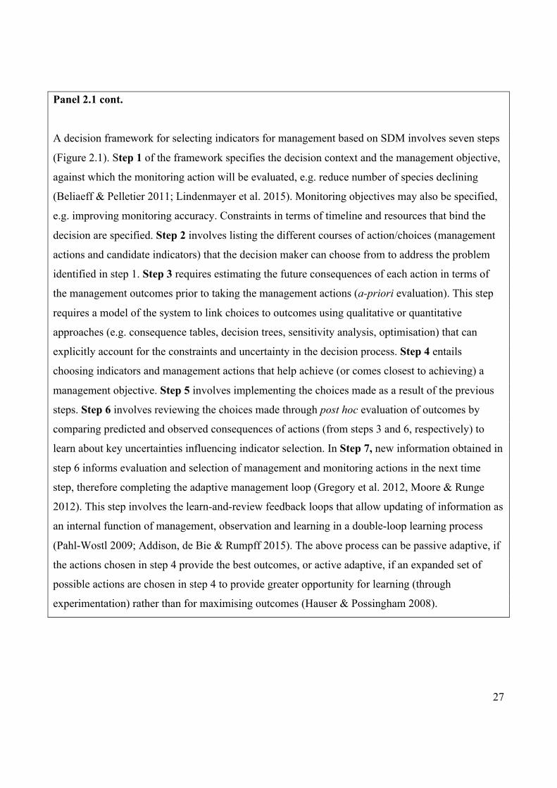
27

Panel 2.1 cont.

A decision framework for selecting indicators for management based on SDM involves seven steps

(Figure 2.1). Step 1 of the framework specifies the decision context and the management objective,

against which the monitoring action will be evaluated, e.g. reduce number of species declining

(Beliaeff & Pelletier 2011; Lindenmayer et al. 2015). Monitoring objectives may also be specified,

e.g. improving monitoring accuracy. Constraints in terms of timeline and resources that bind the

decision are specified. Step 2 involves listing the different courses of action/choices (management

actions and candidate indicators) that the decision maker can choose from to address the problem

identified in step 1. Step 3 requires estimating the future consequences of each action in terms of

the management outcomes prior to taking the management actions (a-priori evaluation). This step

requires a model of the system to link choices to outcomes using qualitative or quantitative

approaches (e.g. consequence tables, decision trees, sensitivity analysis, optimisation) that can

explicitly account for the constraints and uncertainty in the decision process. Step 4 entails

choosing indicators and management actions that help achieve (or comes closest to achieving) a

management objective. Step 5 involves implementing the choices made as a result of the previous

steps. Step 6 involves reviewing the choices made through post hoc evaluation of outcomes by

comparing predicted and observed consequences of actions (from steps 3 and 6, respectively) to

learn about key uncertainties influencing indicator selection. In Step 7, new information obtained in

step 6 informs evaluation and selection of management and monitoring actions in the next time

step, therefore completing the adaptive management loop (Gregory et al. 2012, Moore & Runge

2012). This step involves the learn-and-review feedback loops that allow updating of information as

an internal function of management, observation and learning in a double-loop learning process

(Pahl-Wostl 2009; Addison, de Bie & Rumpff 2015). The above process can be passive adaptive, if

the actions chosen in step 4 provide the best outcomes, or active adaptive, if an expanded set of

possible actions are chosen in step 4 to provide greater opportunity for learning (through

experimentation) rather than for maximising outcomes (Hauser & Possingham 2008).

28

Box 2.1: Definition of search terms used for the review

Indicator species are single or groups of species “used to represent other species or

aspects of the environment to attain a conservation objective” (Landres, Verner &

Thomas 1988, Caro 2010). This includes direct counts of species or composite metrics

such as abundance, density that are estimated by monitoring species or groups of

species (e.g. taxa, guilds, communities). We use the term surrogate species

synonymously for the purpose of this review.

Management implies policies, decisions or actions to prevent or reduce biodiversity

loss (Sparks et al. 2011). This includes conservation management actions, e.g.

establishing protected areas, controlling invasive species; as well as resources

management actions aimed at conserving biodiversity, e.g. fisheries management.

Evaluation implies a qualitative or quantitative assessment or prioritisation of the

indicator with respect to its specified role, e.g. surrogacy for other species, ability to

detect change, ability to track a trend. This might also include comparing indicators

against one another.

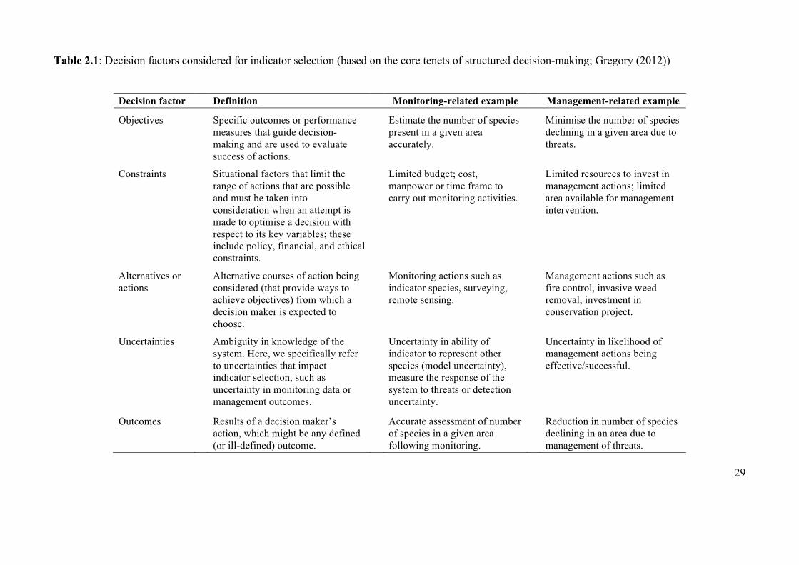
29

Table 2.1: Decision factors considered for indicator selection (based on the core tenets of structured decision-making; Gregory (2012))

Decision factor Definition Monitoring-related example Management-related example

Objectives Specific outcomes or performance measures that guide decision-making and are used to evaluate success of actions.

Estimate the number of species present in a given area accurately.

Minimise the number of species declining in a given area due to threats.

Constraints Situational factors that limit the range of actions that are possible and must be taken into consideration when an attempt is made to optimise a decision with respect to its key variables; these include policy, financial, and ethical constraints.

Limited budget; cost, manpower or time frame to carry out monitoring activities.

Limited resources to invest in management actions; limited area available for management intervention.

Alternatives or actions

Alternative courses of action being considered (that provide ways to achieve objectives) from which a decision maker is expected to choose.

Monitoring actions such as indicator species, surveying, remote sensing.

Management actions such as fire control, invasive weed removal, investment in conservation project.

Uncertainties Ambiguity in knowledge of the system. Here, we specifically refer to uncertainties that impact indicator selection, such as uncertainty in monitoring data or management outcomes.

Uncertainty in ability of indicator to represent other species (model uncertainty), measure the response of the system to threats or detection uncertainty.

Uncertainty in likelihood of management actions being effective/successful.

Outcomes Results of a decision maker’s action, which might be any defined (or ill-defined) outcome.

Accurate assessment of number of species in a given area following monitoring.

Reduction in number of species declining in an area due to management of threats.

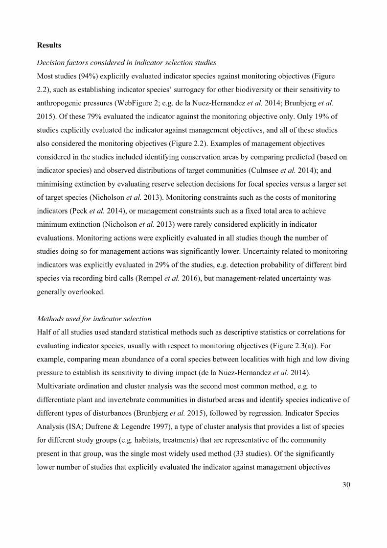
30

Results

Decision factors considered in indicator selection studies

Most studies (94%) explicitly evaluated indicator species against monitoring objectives (Figure

2.2), such as establishing indicator species’ surrogacy for other biodiversity or their sensitivity to

anthropogenic pressures (WebFigure 2; e.g. de la Nuez-Hernandez et al. 2014; Brunbjerg et al.

2015). Of these 79% evaluated the indicator against the monitoring objective only. Only 19% of

studies explicitly evaluated the indicator against management objectives, and all of these studies

also considered the monitoring objectives (Figure 2.2). Examples of management objectives

considered in the studies included identifying conservation areas by comparing predicted (based on

indicator species) and observed distributions of target communities (Culmsee et al. 2014); and

minimising extinction by evaluating reserve selection decisions for focal species versus a larger set

of target species (Nicholson et al. 2013). Monitoring constraints such as the costs of monitoring

indicators (Peck et al. 2014), or management constraints such as a fixed total area to achieve

minimum extinction (Nicholson et al. 2013) were rarely considered explicitly in indicator

evaluations. Monitoring actions were explicitly evaluated in all studies though the number of

studies doing so for management actions was significantly lower. Uncertainty related to monitoring

indicators was explicitly evaluated in 29% of the studies, e.g. detection probability of different bird

species via recording bird calls (Rempel et al. 2016), but management-related uncertainty was

generally overlooked.

Methods used for indicator selection

Half of all studies used standard statistical methods such as descriptive statistics or correlations for

evaluating indicator species, usually with respect to monitoring objectives (Figure 2.3(a)). For

example, comparing mean abundance of a coral species between localities with high and low diving

pressure to establish its sensitivity to diving impact (de la Nuez-Hernandez et al. 2014).

Multivariate ordination and cluster analysis was the second most common method, e.g. to

differentiate plant and invertebrate communities in disturbed areas and identify species indicative of

different types of disturbances (Brunbjerg et al. 2015), followed by regression. Indicator Species

Analysis (ISA; Dufrene & Legendre 1997), a type of cluster analysis that provides a list of species

for different study groups (e.g. habitats, treatments) that are representative of the community

present in that group, was the single most widely used method (33 studies). Of the significantly

lower number of studies that explicitly evaluated the indicator against management objectives

31

(N=21), standard statistical methods were again the most common (Figure 2.3(b)). This was

followed by regression or optimisation in a third of the studies each (e.g. Nicholson et al. 2013).

Methods used to incorporate decision factors in indicator selection

Common selection methods, namely standard statistical methods, ordination and clustering and

regression (Figure 2.3(a)), usually evaluated monitoring rather than management outcomes (Figure

2.4). Infrequently used methods such as optimisation and cost-benefit analysis consistently

accounted for both management and monitoring factors. Objectives are the most frequently

considered factor across indicator selection methods for both the monitoring and the management

component of the indicator selection decision. Actions and their outcomes are the next most

considered factors, although these are much more commonly dealt with in the monitoring

component of the decision, compared with the management component (Figure 2.4). Uncertainties

and constraints are the most infrequently considered decision factors regardless of the selection

method used (Figure 2.4).

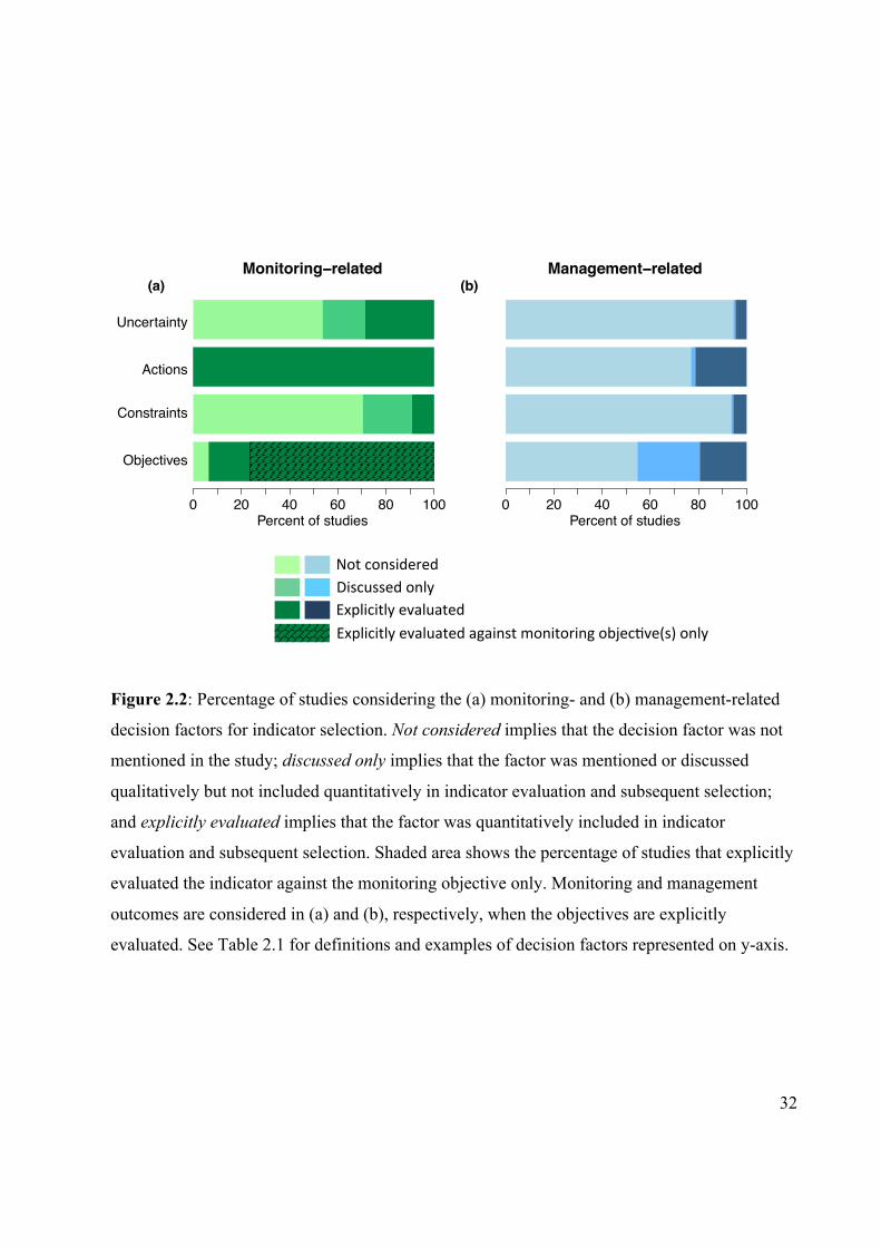
32

Figure 2.2: Percentage of studies considering the (a) monitoring- and (b) management-related

decision factors for indicator selection. Not considered implies that the decision factor was not

mentioned in the study; discussed only implies that the factor was mentioned or discussed

qualitatively but not included quantitatively in indicator evaluation and subsequent selection;

and explicitly evaluated implies that the factor was quantitatively included in indicator

evaluation and subsequent selection. Shaded area shows the percentage of studies that explicitly

evaluated the indicator against the monitoring objective only. Monitoring and management

outcomes are considered in (a) and (b), respectively, when the objectives are explicitly

evaluated. See Table 2.1 for definitions and examples of decision factors represented on y-axis.

(a)

0 20 40 60 80 100

Objectives

Constraints

Actions

Uncertainty

Percent of studies

Monitoring−related(b)

0 20 40 60 80 100Percent of studies

Management−related

Not$considered$Discussed$only$Explicitly$evaluated$Explicitly$evaluated$against$monitoring$objec9ve(s)$only$

33

Figure 2.3: Frequency of methods used for indicator selection in (a) all studies considered in the

review and (b) studies explicitly evaluating the indicator against management outcomes. Categories

used for methods were not mutually exclusive (see Table A1.2 for definitions).

(a)

0 10 20 30 40 50 60Percent of studies

Standard statistical methodsOrdination & clustering

RegressionOther

Elicitation & scoringOptimization

Published sourcesSpecies accumulation/area curves

Cost−benefitScenario modelling

Adaptive management & monitoring

All studies(N=108)

(b)

0 10 20 30 40 50 60Percent of studies

Standard statistical methodsOrdination & clustering

RegressionOther

Elicitation & scoringOptimization

Published sourcesSpecies accumulation/area curves

Cost−benefitScenario modelling


Studies evaluating indicators againstmanagement objectives (N=21)

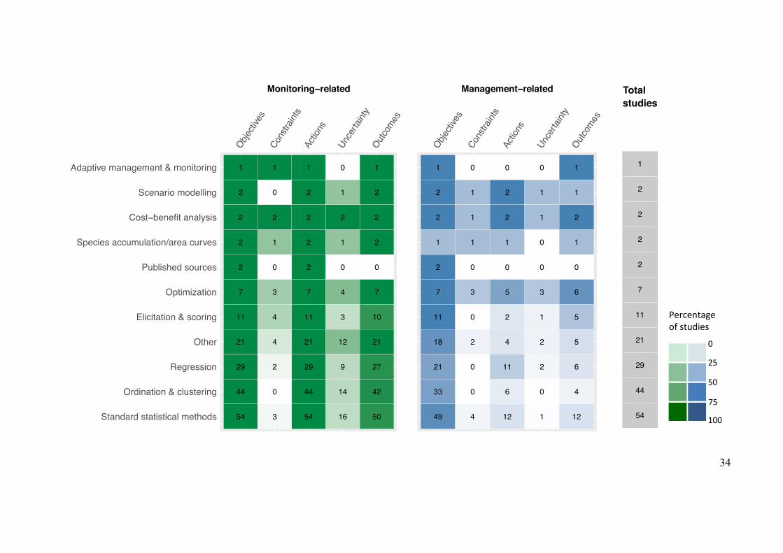
34

0"

25"

50"

75"

100"

Percentage""of"studies"

1

2

2

2

2

7

11

21

29

44

54

1

0

2

1

0

3

4

4

2

0

3

1

2

2

2

2

7

11

21

29

44

54

0

1

2

1

0

4

3

12

9

14

16

1

2

2

2

0

7

10

21

27

42

50Standard statistical methods

Ordination & clustering

Regression

Other

Elicitation & scoring

Optimization

Published sources

Species accumulation/area curves

Cost−benefit analysis

Scenario modelling


Monitoring−related

Objecti

ves

Cons

traint

sAc

tions

Unce

rtaint

yOutc

omes

1

2

2

1

2

7

11

18

21

33

49

0

1

1

1

0

3

0

2

0

0

4

0

2

2

1

0

5

2

4

11

6

12

0

1

1

0

0

3

1

2

2

0

1

1

1

2

1

0

6

5

5

6

4

12

Management−related

Objecti

ves

Cons

traint

sAc

tions

Unce

rtaint

yOutc

omes

54

44

29

21

11

7

2

2

2

2

1

Totalstudies

35

Figure 2.4 (previous page): Decision factors considered by the different methods of indicator

selection. Methods categories (y-axis) were not mutually exclusive. Cell values represent the

number of studies using said method to address a decision factor. Colour gradation represents how

frequently said method is used to address a decision factor (Frequency is calculated as the

percentage of studies using said method to address a decision factor out of the total number of

studies using that method. Numbers in the grey column on the extreme right indicate total number

of studies using a method. E.g. monitoring objectives were considered in 100% of the studies that

used standard statistical methods, while management objectives were considered in 75% of the

studies that used standard statistical methods). Objectives column corresponds to studies where this

factor was clearly defined. Constraints column indicates studies where constraints were explicitly

incorporated when setting the objective. Actions column corresponds to studies where this factor

was clearly defined. Outcomes column corresponds to studies where objectives and actions were

explicitly evaluated (as in Figure 2.2), i.e. outcomes of actions were estimated. Therefore, if a

method was used to estimate outcomes, objectives had to be specified, but explicit statement of

objectives did not necessarily require estimation of outcomes. Uncertainty column implies studies

where actions were explicitly evaluated for one or more uncertainties. Definitions of decision

factors and method categories can be found in Table 2.1 and Table A1.2, respectively.

Discussion

Limitations of current approaches

A key reason for monitoring biodiversity is to reduce uncertainty regarding which management

actions to implement and what the outcomes might be for biodiversity (Possingham et al. 2012).

Despite this need, our review demonstrates that indicator species proposed in the literature are

generally not evaluated based on whether they can effectively inform and improve management

decisions. In fact, most studies ignore the management component altogether (Figure 2.2). The

majority of studies use indicator selection methods aimed at improving monitoring efficiency alone,

for instance evaluating whether an indicator is a reliable surrogate for another species or for an

ecological community (Figure A1.2). This indicates that management is only considered in a

limited way and proposed indicators are not being evaluated correctly in terms of their ultimate

performance (i.e. management outcomes), but rather on proximate measures alone (i.e. monitoring

outcomes) (Figure 2.4). As such, indicator species may lack pragmatic utility in effectively

informing state-dependent management decisions (Lindenmayer, Piggott & Wintle 2013). Overall,

36

only a few indicator selection methods were able to account for all of the decision factors even for

just the monitoring or just the management-related component of the decision (Figure 2.4) (but see

Nicholson et al. (2013) for an example that considers all factors except the monitoring constraints).

While monitoring constraints (e.g. specifying an acceptable level of risk or uncertainty, monitoring

budget) help limit the suite of monitoring strategies to choose from, management constraints (e.g.

resource limitations for management actions) help specify realistic and achievable management

objectives. Ignoring management constraints leads to the possibility of fundamentally different

management objectives and hence outcomes, ones that may potentially lead to the selection of

different indicators. For instance, improving species persistence under an unlimited budget may not

even require optimal management and monitoring decisions because there are enough resources to

do everything. On the other hand, management under resource constraints requires indicators that

can inform on the efficacy of feasible management actions. By ignoring uncertainties, proposed

indicators may overestimate the benefit of monitoring to improve decisions or may not be cost-

effective (Lyons et al. 2008).

In our view, there are two reasons indicator research continues to be rooted in the traditional

approach of selecting indicators to adequately represent natural systems, rather than evaluating

them for multiple decision factors (e.g., objectives, actions and uncertainties; Figures 2.2 and 2.4).

Firstly, applying SDM and decision-analysis tools (Raiffa 1968; Gregory 2012) to monitoring

decisions is a relatively new area for conservation science. Even though the analytic methods used

for SDM such as cost-benefit and optimisation methods have been around for some time (e.g.

Gerber et al. 2005), their uptake in conservation science has been slow relative to other disciplines

such as medicine and economics. This explains why even simple methods such as cost-

effectiveness analysis to compare the relative outcomes and costs of different indicator choices are

rarely used (Figure 2; but see Tulloch, Possingham & Wilson 2011). Secondly, decision-analytic

approaches rely heavily on the use of mathematical models that require significant technical

expertise (Shea & NCEAS Working Group on Population Management 1998; Sarkar et al. 2006).

Users may find these approaches technically challenging, time-consuming or they may be

unfamiliar with the underlying principles and mathematical models (Addison et al. 2013). As such,

researchers may favor simpler and well-documented methods such as regression, correlations or

ordination analysis for indicator selection (Figure 2.3). However, these methods do not of

themselves constitute a decision-making framework (Burgman et al. 2012; Gregory 2012), and

therefore do not help evaluate multiple decision factors (e.g., objectives, actions and uncertainties).

37

For example, if multiple indicators show similar trends in response to a management action, there is

no way of selecting between them without considering other aspects such as costs, budgets and

uncertainties in the responses (Tulloch et al. 2013).

The way forward

We propose that indicator selection needs to focus on three key areas for future research: (1)

framing indicator selection problems within a clear decision context (steps 1 and 2 in Figure 2.1);

(2) developing better indicator selection methods focused on improving management outcomes

(step 3 in Figure 2.1); and (3) incorporating iterative learning regarding key uncertainties in the

indicator selection process to improve indicator choices over time (step 7 in Figure 2.1).

Clear decision context

When intended to inform management decisions, monitoring is not an end in itself but derives its

purpose and value from the decision context and the subsequent improvements in decision-making

(Nichols and Williams 2006). The need to make decisions about indicator selection therefore comes

from identifying (and articulating) a conservation or management problem that calls for monitoring

to improve management outcomes (McDonald-Madden et al. 2010a). This means that we need to

move beyond the much-cited trade-off between measurement accuracy and practical constraints of

monitoring indicators (Lindenmayer et al. 2015), to a full clarification of the management decision

factors that govern indicator choice (i.e. formulating the problem at steps 1 and 2 in Figure 2.1).

Alternative indicators can then be evaluated to choose the ones that best help achieve the

management objective given the constraints. While monitoring objectives may also be specified,

e.g. improving monitoring accuracy, we suggest that these are secondary to the management

objective when indicators are being selected for management decision-making.

Indicator selection methods focused on improving management outcomes

In order to evaluate the benefit of indicators for management, we need indicator selection methods

that are closely aligned with the specifics of the management problem (i.e., objectives, constraints,

actions and uncertainty). These methods must be capable of assessing the outcomes of choosing

alternative indicators for management decision-making, while accounting for the constraints and

uncertainties in the decision process (i.e. a-priori evaluation at step 3 in Figure 2.1). Examples of

such methods that have been used for indicator selection include optimisation, cost-effectiveness

analysis and adaptive management and monitoring, but these appear infrequently in the literature

38

(Figure 2.3). Other methods such as value of information (VOI), an approach to identify the best

way to expend efforts on collecting data to improve a decision through reducing uncertainty, apear

not to have been used for indicator species selection (but see Pannell & Glenn 2000).

Methods such as VOI, though complex, can be used to identify simple principles for monitoring and

indicator selection. For example, Pannell and Glenn (2000) use VOI for economic valuation and

prioritisation of ‘sustainability indicators’ in agriculture science and propose criteria for choosing

between indicators for a given management problem. These methods can be enhanced by

developing spreadsheet tools and user-friendly software to make them more accessible, thereby

encouraging their uptake in conservation (e.g. Canessa et al. 2015). Simpler methods such as

control charts (graphics to show temporal changes in a system/process) could also help convey

monitoring benefits in simple graphics and indicate any potential need for management (Burgman

et al. 2012). However, they need to be accompanied by clearly specified trigger points and

management interventions (Lindenmayer, Piggott & Wintle 2013) so that subsequent management

outcomes can be incorporated in indicator evaluation. Most importantly, however, we need to better

communicate the benefit of using the right methods for indicator selection (Addison et al. 2013) as

well as the risks of using methods that fail to link monitoring actions, i.e. indicators, to management

outcomes (Lyons et al. 2008).

Iterative selection

Existing frameworks for indicator selection (Pannell & Glenn 2000; e.g. Beliaeff & Pelletier 2011;

Nicholson et al. 2012; Lindenmayer et al. 2015) and the SDM literature collectively provide

guidance on how to systematically consider the key decision factors and establish a robust,

management-oriented decision framework for indicator selection (Figure 2.1). Furthermore,

adaptive management and iterative monitoring frameworks can help incorporate learning and

updating decisions over time by explicitly accounting for uncertainties in the decision process, e.g.

in the response of an indicator to management or in management effectiveness (Ringold et al. 1996;

Lyons et al. 2008). This allows indicator choices to be reviewed and updated over time and for

indicator selection to respond to the dynamic nature of ecological systems and decision processes,

including the possibility of changing objectives and management actions (e.g. Nicholson et al.

2012; Lindenmayer et al. 2015). An iterative approach, therefore, provides a marked improvement

over current selection approaches that ignore the fact that, as is the case for management decision-

39

making, monitoring decisions too may change over the course of a management program (Williams,

Eaton & Breininger 2011).

Choosing useful indicators is crucial for effectively managing biodiversity, as indicators provide

information capable of changing the course of management decisions. The risks of failing to

correctly identify relevant indicators for conservation are high, potentially leading to irreversible

consequences for biodiversity such as extinctions or loss of critical habitat (Lindenmayer, Piggott &

Wintle 2013). Our review shows that indicator selection continues to focus on improving

monitoring efficiency rather than improvements in management effectiveness. Indicator species

chosen to achieve a particular monitoring objective may be recommended for complex management

decisions that often involve multiple objectives, without adequate testing of their performance to

improve decision-making. To correct for this, when choosing indicator species, decision-makers

should explicitly consider the decision context rather than relying purely on the ecological validity

of indicators. A decision framework for indicator selection that draws on the core tenets of SDM

provides a distinct advantage over ad-hoc selection methods because it can help ensure that

indicators are relevant to the decision process, lead to improvements in management decisions and

enable cost-effective spending of scarce resources.

Acknowledgements

This research had funding support from the Australian Research Council Centre of Excellence for

Environmental Decisions and the School of Geography, Planning and Environmental Management

at the University of Queensland. We thank Ascelin Gordon for valuable feedback on earlier drafts

of the manuscript and Rebecca Runting for help with data extraction methodology.

40

The value of monitoring species to

manage multiple threats

Under review in Methods in Ecology and Evolution

41

Chapter three – The value of monitoring species to manage multiple

threats

Abstract

Making effective management decisions is challenging in multi-species, multi-threat systems

because of uncertainty about the impacts of different threats on different species. To inform

management decisions, we often monitor species to detect trends over time and to learn about

threatening processes. However, which species to monitor and how to best inform management can

be difficult to determine. Value of information (VOI) is an approach for identifying the best way to

monitor to resolve uncertainty and hence improve a management decision. We used VOI to

investigate how monitoring alternative species subject to multiple threats improves our ability to

inform the management of threats in a multi-species system. Specifically, we compared the

effectiveness of passive monitoring (monitoring species without experimentation) with

experimental monitoring (monitoring with experimentation to explicitly learn about threats). We

then applied the approach to two contrasting case studies of managing threats for declining

mammals in Western Australia. Our case studies show that passive monitoring provides almost no

information for targeted decision-making when managing multi-species, multi-threat systems under

constrained resources. Experimental monitoring provides much higher benefits for managing

multiple threats and species simultaneously in terms of conservation outcomes. We identify the key

ecological and economic factors that drive the choice of the optimal monitoring strategy under the

experimental approach. The case studies emphasise that optimal monitoring choices are not always

intuitive and depend on the interaction between management budgets, management costs and

threats. It is in these situations where our VOI approach is most useful to evaluate how changes in

each of the decision parameters change monitoring choices in multi-species, multi-threat systems.

Our study demonstrates a novel application of the VOI approach to multi-species, multi-threat

management problems. It allows managers to critically evaluate monitoring decisions in the face of

uncertainty while explicitly accounting for the improvement in management decisions. A key

insight from our application of VOI to the monitoring of multi-species multi-threat systems is that

managers need to carefully consider the decision context when selecting which species to monitor

to inform management. Decisions that only consider ecological factors are likely to lead to inferior

monitoring and therefore management outcomes.

42

Introduction

Most species are impacted by multiple threats that together play a significant role in observed

species declines (Brook, Sodhi & Bradshaw 2008). To reduce or reverse declines due to these

threats, conservation efforts need to be prioritised and allocated strategically across multiple threats

(Auerbach, Tulloch & Possingham 2014). This approach requires information on the impacts of

threats and the consequences of alternative threat reduction activities, but these are often uncertain

(Evans, Possingham & Wilson 2011). Monitoring species to learn about multiple threats, however,

is not straightforward because threats often act in tandem, thus potentially confounding the ability

to separate the effect of each threat (Breitburg et al. 1998). When the conservation objective is to

conserve multiple species subjected to multiple threats, the challenge is even greater. In these cases,

monitoring decisions need to account for cumulative threats as well as the link between each threat

and the response of different species to these threats.

Effective monitoring for conservation decision-making when resources are limited needs to focus

specifically on gaining information that informs and improves management outcomes (McDonald-

Madden et al. 2010). Long-term monitoring programs like the UK Breeding Bird Survey (Robinson

et al. 2016) monitor species to assess changes and establish baseline data against which efforts to

reduce biodiversity loss may be evaluated. This type monitoring can indicate directionality or

magnitude of observed trends, providing invaluable ecological insights (Wintle, Runge & Bekessy

2010). Monitoring species, as well as threats, to establish statistical associations between trends in

numbers and threats can reveal the relative importance of threats and the associated management

actions (e.g. Siriwardena, Calbrade and Vickery 2008). Alternatively, species can be monitored in

combination with experimental manipulations of the threats, such as controlling predator abundance

or the degree of disturbance, to learn about the consequences of management (Walters & Holling

1990; e.g. U.S. Fish and Wildlife Service 2015). In this study, we evaluate monitoring as a means of

quantifying the effectiveness of management in multi-species, multi-threat systems.

There are many examples of monitoring or modelling the response of species to multiple threats and

their management (e.g. Stephens et al. 2003; Siriwardena, Calbrade & Vickery 2008). However,

these studies evaluate the effectiveness of alternative management rather than monitoring actions.

There is also extensive literature on techniques to evaluate and prioritise the most effective actions

for management, such as cost-effectiveness analysis, project prioritisation protocols, and

43

management strategy evaluation (e.g. Joseph, Maloney & Possingham 2008; Bunnefeld, Hoshino &

Milner-Gulland 2011), but similar studies for evaluating the effectiveness of alternative monitoring

actions for management decision-making are limited (but see Runge, Converse & Lyons 2011;

Tulloch, Possingham & Wilson 2011). In particular, few studies evaluate the effectiveness of

alternative monitoring strategies (such as monitoring species only versus combining experimental

manipulations with monitoring) to resolve uncertainty to inform threat management. We also know

little about the determinants of the best species to monitor to inform threat management.

Value of information (VOI) analysis provides a useful method to compare the benefits of alternative

monitoring decisions. It has been used in disciplines, such as economics (Radner & Stiglitz 1984),

health sciences (Yokota & Thompson 2004), agriculture (Pannell & Glenn 2000) and only recently

for conservation decision-making (Runge, Converse & Lyons 2011; Maxwell et al. 2015). VOI is

defined as the difference between the expected value of outcomes for an optimal management

decision made after gaining new information, compared to one made on the basis of prior

understanding (Raiffa & Schlaifer 1961). It is based on the premise that gaining new information

can reduce uncertainty to improve decision-making and explicitly considers the optimal

management decision that arises from existing information (Canessa et al. 2015). However,

obtaining new information may not always improve outcomes sufficiently to compensate for the

costs incurred by gaining the information (McDonald-Madden et al. 2010a).

We demonstrate the use of VOI analysis to identify monitoring strategies that inform decisions

about multiple threat management when multiple species are at stake. We first develop an approach

to compare the value of monitoring alternative species to learn about threats affecting the species

and their responses to management interventions. We then quantify the relative benefit of different

monitoring approaches (i.e. monitoring just species or monitoring with experimental manipulation

of threats) for decision-making, and identify key drivers of the choice of species to monitor and the

choice of experimental manipulation. We illustrate the utility of the approach for real-world

conservation decisions using two case studies focussed on the management of terrestrial mammal

species in Western Australia.

44

Methods

We focus specifically on two types of monitoring strategies, monitoring while experimentally

manipulating the system (Walters & Holling 1990) versus monitoring without experimentation

(Lindenmayer & Likens 2010). We subsequently refer to these as experimental monitoring and

passive monitoring, respectively. We consider a one time-step adaptive management problem but

the terms themselves are only used to describe different types of monitoring and are not meant to

convey passive or active AM, respectively.

In the following sections we explain the multi-species multi-threat study system, the management

decision problem and the VOI method used to evaluate the benefit of monitoring species. We then

describe the case study applications. See Appendix 2.1 for a complete list of parameter notations

used in the VOI analysis described below.

A stylised multi-species multi-threat system

We considered a system in which species are subjected to threatening processes (Figure 3.1a), and

where a manager wants to reduce the number of species in decline by managing the threats present

in the system. Working with limited resources, she must choose optimal management actions, but

she is unsure which threats are causing declines in which species. To inform her decision, she

decides to monitor species declines but resource constraints do not allow for monitoring every

species. Therefore, she needs to identify the most cost-effective species so as not to waste

resources. She also considers monitoring using experimental designs to selectively learn about the

effect of each threat on each species.

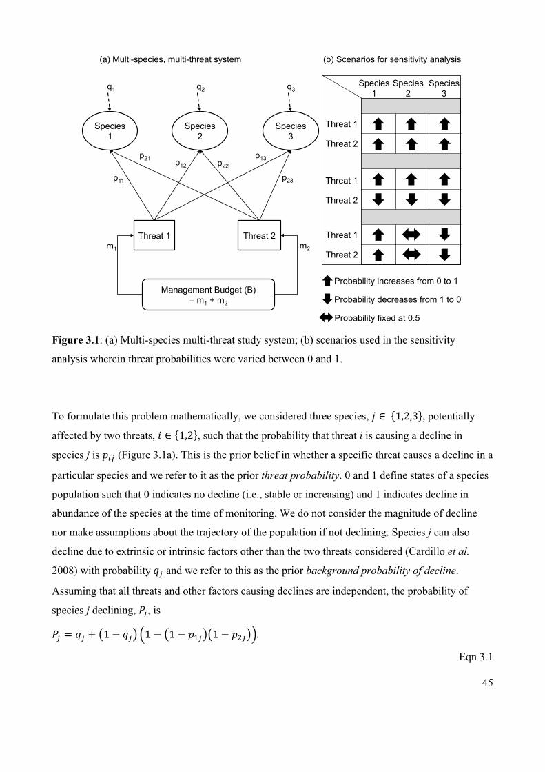
45

Figure 3.1: (a) Multi-species multi-threat study system; (b) scenarios used in the sensitivity

analysis wherein threat probabilities were varied between 0 and 1.

To formulate this problem mathematically, we considered three species, ! ∈ 1,2,3 , potentially

affected by two threats, ( ∈ 1,2 , such that the probability that threat i is causing a decline in

species j is )*+ (Figure 3.1a). This is the prior belief in whether a specific threat causes a decline in a

particular species and we refer to it as the prior threat probability. 0 and 1 define states of a species

population such that 0 indicates no decline (i.e., stable or increasing) and 1 indicates decline in

abundance of the species at the time of monitoring. We do not consider the magnitude of decline

nor make assumptions about the trajectory of the population if not declining. Species j can also

decline due to extrinsic or intrinsic factors other than the two threats considered (Cardillo et al.

2008) with probability,+ and we refer to this as the prior background probability of decline.

Assuming that all threats and other factors causing declines are independent, the probability of

species j declining, -+, is

-+ = ,+ + 1 − ,+ 1 − 1 − )1+ 1 − )2+ .

Eqn 3.1

Variability in species

Variability in threats

Homogeneous threats

Species1

Species2

Species3

Threat 1 Threat 2

p11

p12 p13 p21 p22

p23

Management Budget (B) = m1 + m2

q1 q2 q3

m2 m1

Probability increases from 0 to 1

Probability decreases from 1 to 0

Probability fixed at 0.5

Species 1

Species 2

Species 3

Threat 1

Threat 2

Threat 1

Threat 2

Threat 1

Threat 2

(a) Multi-species, multi-threat system (b) Scenarios for sensitivity analysis

46

This implies that a species j may decline due to factors other than the two threats with probability ,+

or, in the absence of other factors causing declines, species j declines due to the one or both threats

with probability 1 − ,+ 1 − 1 − )1+ 1 − )2+ . The term 1 − 1 − )1+ 1 − )2+ ensures

that the species will decline if at least one of the threats is causing a decline. We have ignored the

possibility of a species declining due to a combination of the target threats and other (background or

non-modelled) threats, which can be easily incorporated as a third term in the above equation.

The decision problem

Management objective

We assumed that the management objective is to minimise the expected number of species

declining.

Management actions and constraints

We assumed that the manager has a limited budget available for management, B, which is split

between managing the two threats. If 41 and 42 are the amounts invested in management of threat

1 and threat 2, respectively, then 5 = 41 +42. We also assume that management actions cannot

influence the background probability of decline, ,+. We assume m1 and m2 to be one-off decisions

and as such we did not explicitly consider a time component in the model.

Model uncertainty

There is uncertainty in the system as to whether a threat causes a decline in a species, which is

characterised by the prior threat probabilities. However, this can also be represented as model

uncertainty in terms of the 64 different combinations (or hypotheses) of how two threats cause

declines or no declines in each of the three species. Based on this the prior probability of model s

being the true model,Pr 8 , for each of the 64 models can be written as functions of the prior

probabilities )*+,

Pr 8 = 9*+: )*+ + 1 − 9*+

: 1 − )*+

;

+<1

2

*<1

Eqn 3.2

47

where 9*+: = 0 if threat i does not cause a decline in species j in model s and 9*+

: = 1if threat i

causes a decline in species j in model s. Therefore, 9*+: represents the true state for species i under

threat j in model s while )*+ represents our belief in the true state.

Value of information analysis

Calculating the value of perfect information

The expected value of perfect information (EVPI) provides the upper bound on the VOI and is the

expected benefit of eliminating uncertainty entirely. We specified the EVPI for the decision

problem as

>?-@ = − minDE

F: 41

GH

:<1

Pr 8 + minDE

F: 41 Pr 8

GH

:<1

Eqn 3.3

where the first term gives the expected outcome of the optimal decision under perfect information,

while the second term gives the expected outcome of the optimal decision under uncertainty about

the true model (Runge, Converse & Lyons 2011). 41is the amount invested in managing threat 1

such that 41 ≥ 0, Pr 8 is the probability that model s is the true model and the objective function,

F: 41 , is the expected number of species declining under investment 41for model 8. As the

management optimisation problem is a minimisation, we multiplied the standard EVPI equation by

-1 so that EVPI is positive. Therefore,

F: 41 = ,+ + 1 − ,+ 1 − 1 − 91+(:) L1 − 41

L11 − 92+

(:) L2 − 42

L2

;

+<1

Eqn 3.4

where L1and L2are the costs of eliminating threat 1 and 2 such that 41 ≤ L1,42 ≤ L2 and 42 =

5 −41. Equation 3.4 implies that the expected number of species declining is reduced as a result

of the amount invested in managing the threats in the system; and assumes that investment in

managing threat ( ∈ 1,2 reduces the probability (not magnitude) of threat i causing a decline in

species ! in a linear fashion up until 4* = L* at which point the probability of decline due to threat i

is zero. We found an analytical solution to the first term of equation 3.3 using Lagrange

minimisation (Bertsekas 1982) in Mathematica Version 10 (Wolfram Research 1988-2015)

(Appendix 2.2) and a numerical solution to the second term.

48

Calculating the value of passive and experimental monitoring

Since we can only obtain a sample of information from monitoring that reduces rather than

eliminates uncertainty in most cases, we turn to the expected value of sample information (EVSI)

(Runge, Converse & Lyons 2011),

>?N@ = − Pr O minDE

F: 41 Pr 8 O

GH

:<1

+ minDE

F: 41 Pr 8

GH

:<1O

Eqn 3.5

where x represents the data collected during monitoring,-P O is the prior probability of observing

x, -P 8 O is the probability that model s is the true model given x has been observed (i.e. the

posterior probability), and the outer sum in the first term is over all possible discrete values for x.

The first term in equation 3.5 gives the expected outcome of the optimal decision under imperfect

information (i.e. for each possible value of sample information), while the second term is the same

as in equation 3.3.

Considering a one-time step adaptive management problem, management actions in the first time

step are implicit. In both types of monitoring, passive and experimental, prior probabilities of

decline (pij) are updated following monitoring in the first time step and then the optimal

management decision is made in terms of the investment in managing threat 1 versus threat 2 (m1

versus m2) i.e. subsequent management actions for the next time step are identified. VOI presents a

standard decision analytical approach, where an a-priori belief in the hypotheses (here, relating to

the cause of decline) is used to select the best management action and monitoring is then used to

compare predictions to observations and to update this belief. In the passive monitoring case, we

assume we monitor one or two species only and detect whether the species is declining or not

without error (i.e. Type I and Type II errors are zero). We assume no observation error for

tractability. Therefore, x is a vector of length equal to the number of species monitored, with an

entry of 1 if a decline is detected and an entry of 0 if a decline is not detected. In the experimental

monitoring case, we monitor species at a control and an experimental site, with one of the threats

eliminated at the experimental site. Here the decision is not only about which species to monitor but

also which threat to experimentally manage. In this case x is a matrix of size number of species

monitored by two (i.e. one set of monitored outcomes for the control site and one set of monitored

outcomes for the experimental site). Once again, the entries are 1 or 0 depending on whether a

49

decline is detected or not. A monitoring strategy under the passive approach comprised of selecting

species to monitor while under the experimental approach comprised of selecting a combination of

species to monitor and a threat to manage experimentally. Optimal monitoring strategies were

identified as those that provided the highest EVSI. We used a constrained nonlinear multivariable

optimisation algorithm [‘fmincon’ function in MATLAB Version R2015b (Mathworks 1984–

2015)] to estimate EVPI and EVSI. For detailed EVSI equations, their derivation and the MATLAB

code, see Appendix 2.3 and 2.6.

Scenario and sensitivity analysis

We set up three scenarios of threats causing declines in species by varying the prior threat

probabilities (Figure 3.1b): 1) Homogeneous threats where all threat probabilities are the same; 2)

Variability among threats where probabilities of the two threats causing declines are different, but

the probability of a given threat causing decline is the same for all three species; and 3) Variability

among species where probabilities of the two threats causing declines are the same for a given

species, but these differ among species. We then tested, for each scenario, the sensitivity of the

EVSI and the best monitoring strategy to the decision parameters, i.e. available management

budgets, relative costs of threat management and the background probability of decline.

Case studies

We applied our approach to two management case studies from Western Australia. For each, we

estimated the EVSI for monitoring species (single or pairs) under the experimental and passive

approach. We then compared monitoring strategies to identify best choices for combining species

monitoring with experimental manipulation of the system to learn about the threats.

Our first case study was in the Pilbara region of northwestern Australia, which is home to a number

of threatened and endemic species. The area is under growing pressures from over-grazing, invasive

species, altered fire and hydrological regimes and extractive mining (McKenzie, van Leeuwen &

Pinder 2009). Based on an existing region-wide assessment of management strategies for mitigating

the effects of multiple threats on Pilbara’s biodiversity (Chadès et al. 2015), we selected three co-

occurring target species that are being monitored or considered for monitoring in the study region:

Macrotis lagotis (greater bilby), Dasyurus hallucatus (northern quoll) and Rattus tunneyi (pale

field-rat). To downscale the problem, we considered threats only for the Fortescue subregion of the

50

Pilbara, namely: over-grazing due to feral ungulates and domestic herbivores and altered fire

regimes, both of which continue to degrade the Pilbara at rates equivalent to other arid pastoral

regions of Australia (McKenzie, van Leeuwen & Pinder 2009). We considered two management

strategies: (1) fire management; and (2) combined feral ungulate and domestic herbivore

management. Species persistence under different management strategies available in Chadès et al.

(2015) and insights from published studies (see Woinarski et al. 2010) indicate that threats

influence all species negatively, though the degree of impact may be variable. Details on actions

constituting each strategy and their associated costs were also obtained from Chadès et al. (2015).

See Appendix 2.4 for further details.

Our second case study was in an internationally recognised global biodiversity hotspot, the Fitz-

Stirling – fragmented remnant patches of woodland and heathland in agricultural land stretching

70km from the Stirling Ranges to Fitzgerald River National Parks in southwestern Australia. We

considered three target species: Trichosurus vulpecula (western brushtail possum), Macropus

eugenii (tammar wallaby) and Isoodon obesulus (southern brown bandicoot or quenda), under two

key threats: the invasive predator, Vulpes vulpes (European red fox) and altered fire regimes.

Management strategies for recovering mammals in several large protected areas in the region

involve poison baiting for foxes, and active fire management to prevent too-frequent fires

(controlled burning and other activities) as well as fire suppression when wildfires occur. Altered

fire regimes result in declines in most species including T. vulpecula and I. obesulus, but some

grazing species such as M. eugenii may benefit from food replenishment through grass growth and

fruiting of small bushes following fires, therefore showing an increase following some types of fires

(Christensen 1980). We used data from published and unpublished studies since the 1970s that

recorded changes in target species abundance for: (1) fox baiting; (2) fox threat without

management; (3) fire management (suppression and prevention); and (4) fire threat without

management (uncontrolled wildfires and changed fire regimes). We obtained the species decline

probabilities under different management actions using the approach detailed in Tulloch, Chadès

and Possingham (2013). We estimated costs of management based on expert elicitation (Bush

Heritage Australia and the Department of Parks and Wildlife Australia) and information available in

previous studies (see Appendix 2.4).

51

Results

Scenario and sensitivity analysis

In general, EVPI and EVSI vary with the relative budget (i.e. percentage of the total budget

required for completely managing both threats) and threat probabilities (Figure 3.2). Both are zero

at 0 and 100% relative budgets, and maximum between these extremes. Maximum EVSI for passive

monitoring is close to zero in all scenarios for all values of relative budget. EVSI is significantly

higher under experimental monitoring, achieving up to 54% of EVPI when monitoring one species

and 76% when monitoring two species (Figure 3.2).

When monitoring two species experimentally, certain combinations of decision parameters lead to

low EVSI, indicating low benefit from monitoring (Figure 3.3). EVSI is zero when relative cost for

managing one threat is very high and that for the other is very low, and threat probabilities are close

to zero or one. Between these extremes, EVSI depends on the interaction between the variables.

When threat probabilities are the same for all species and threats (scenario 1), EVSI decreases as

the relative costs of managing the two threats become different. At intermediate and high budgets,

EVSI is lower at high values of threat probabilities compared to at low values of threat

probabilities, but this is not the case at low budgets. When there are differences in threat

probabilities among threats (scenario 2), EVSI is low when the relative cost of managing a threat is

low and the probability of that threat causing a decline is high and vice-versa (Figure 3.3). In this

case, relative budget has little influence on EVSI because it is driven primarily by the interaction

between cost and threat probability. When there are differences in threat probability among species,

but not among threats (scenario 3), EVSI again decreases with increase in difference between

relative costs of managing the two threats but it does not vary much in response to changing threat

probabilities and relative budget. The same general patterns emerge when monitoring one species

under the experimental approach, but EVSI is lower overall (Figure A2.1). Results presented here

are for low values of background probability of decline (q = 0.01), essentially representing a closed

system of species and threats. EVSI is negatively related to the background probability of decline,

reducing to zero at very high values of qj.

We also compared the performance of alternative experimental monitoring strategies under each

scenario for relative budget fixed at 50% of the total budget required to completely manage both

threats. The choice of best monitoring strategy changes with relative costs of managing threats and

52

threat probabilities (Figure 3.4). In scenarios 1 and 2, the benefits of experimentally monitoring any

two of the three species are equal (i.e. equal EVSI) for all values of threat probability. Therefore,

threat probability has no influence on the optimal strategy in these cases. However, the relative cost

of management drives the choice of which threat to experimentally manage. In scenario 3,

monitoring of different species provide different benefits (i.e. different EVSI). Here, threat

probability drives the choice of which species to monitor and the cost of managing threats drives

the choice of which threat to experimentally manage. Overall, EVSI is highest when there are

differences in threat probability among threats (scenario 2). Selecting the best monitoring strategy,

for instance in scenario 2 (Figure 3.4) the optimal strategy of monitoring species while

experimentally managing threat 1 can result in a reduction of up to 0.18 expected number of species

declining as opposed to monitoring while experimentally managing threat 2, the latter resulting in a

reduction of up to 0.11 expected number of species declining.

53

Figure 3.2: Value of information (EVPI, EVSI) as relative budget increases. VOI (y-axis)

expressed as the reduction in expected number of species declining and relative budget (x-axis)

expressed as a percentage of the total budget required for completely managing both threats.

Scenarios tested at fixed relative cost of managing threats (each 50% of total budget), low

background probability of decline (0.01) and fixed threat probabilities (as specified in figure).

0

0.1

0.2

0.3

0.4

0

0.1

0.2

0.3

0.4

0 20 40 60 80 1000

0.1

0.2

0.3

0.4

Scenario 2: Variability in threats

Scenario 3: Variability in species

Relative budget

Valu

e of

info

rmat

ion

(Red

uctio

n in

exp

ecte

d nu

mbe

r of s

peci

es d

eclin

ing)

Scenario 1: Homogeneous threats

Threat x Species matrix of prior threat probabilities:

EVSI for experimental monitoring of 2 species

EVSI for experimental monitoring of 1 species

EVSI for passive monitoring of 1 species

EVSI for passive monitoring of 2 species

EVPI

Key:

54

Figure 3.3: Benefit (EVSI) of experimentally monitoring two species. EVSI expressed as reduction

in expected number of species declining under best monitoring strategy. Relative cost of managing

threat 1 (x-axis), expressed as a percentage of the total budget required to completely manage both

threats (relative cost for threat 2 decreases from 100 to 0% on x-axis). Threat probabilities (y-axis)

i.e. probability of both threats causing declines in all species increases from 0 to 1 (scenario 1);

relative probability of threat 1 causing declines in all three species increases from 0 to 1 and relative

probability of threat 2 causing decline in all three species decreasing from 1 to 0 (scenario 2);

probability of both threats causing declines increases from 0 to 1 for species 1, decreases from 1 to

0 for species 3 and is fixed at 0.5 for species 2 (scenario 3). Scenarios tested at fixed relative

budgets (as specified in figure) and low background probability of decline (0.01).

0 50 1000 50 100

00.20.40.60.81

00.20.40.60.81

0 50 1000

0.20.40.60.81


Scenario 2: Variability among threats

Scenario 3: Variability among species

Relative cost of managing threat 1

Thre

at p

roba

bilit

ies

Low budget (25%) Intermediate budget (50%) High budget (75%)

For a

ll th

reat

s Fo

r thr

eat 1

Fo

r spe

cies

1

EVSI (2 species monitoring, experimental approach)

0 0.05 0.1 0.15 0.2 0.25

55

Figure 3.4: Performance of two species experimental monitoring strategies. Coloured lines indicate

which species was/were monitored (as per legend). Solid lines indicate that the species was/were

monitored under experimental management of threat 1 and dotted lines indicate that the species

was/were monitored under experimental management of threat 2. EVSI (y-axis) expressed as the

reduction in expected number of species declining. Threat probabilities (y-axis) i.e. probability of

both threats causing declines in all species increases from 0 to 1 (scenario 1); relative probability of

threat 1 causing declines in all three species increases from 0 to 1 and relative probability of threat 2

causing decline in all three species decreasing from 1 to 0 (scenario 2); probability of both threats

causing declines increases from 0 to 1 for species 1, decreases from 1 to 0 for species 3 and is fixed

at 0.5 for species 2 (scenario 3). Scenarios tested at fixed relative budget (50% of total budget

required to completely manage both threats), low background probability of decline (0.01), and

fixed relative cost of managing threat 1 (as specified in figure). See Appendix 2.5 for corresponding

figures at low and high relative budgets (Figure A2.2).

0

0.05

0.10

0.15

0.20

0

0.05

0.10

0.15

0.20

0 0.2 0.4 0.6 0.8 10

0.05

0.10

0.15

0.20

0 0.2 0.4 0.6 0.8 1

@ Medium budget (50%)

Low$cost$of$$managing$threat$1$$

EV

SI

Threat probabilities

High$cost$of$$managing$threat$1$

Manage threat 1 Manage threat 2

Monitor species 1 & 2 Monitor species 1 & 3 Monitor species 2 & 3

Monitoring strategy: Scenario 1: Homogeneous threats



56

Case studies

In the Pilbara case study, passive monitoring provides virtually no information for decision-making

(Figure A2.3a in Appendix 2.5). When experimentally monitoring one species, M. lagotis is

selected as the optimal species for all relative budget values. The optimal experiment changes from

managing over-grazing to managing fire as the relative budget available for management increases

beyond 60% of the total budget required to manage both threats completely. When experimentally

monitoring two species, M. lagotis and D. hallucatus are optimal for all relative budget values, and

managing grazing is the optimal experiment for all relative budget values.

In the Fitz-Stirling case study, passive monitoring of one or two species and experimental

monitoring of one species provide equally low benefit (Figure A2.3b). When experimentally

monitoring one species, T. vulpecula is optimal at relative budget values close to 0 and 50%, but

selection switches to I. obesulus between these values. When experimentally monitoring two

species together, I. obesulus and T. vulpecula provide the highest benefit, and managing fire is the

optimal experiment for all values of relative budget. Experimentally monitoring two species,

namely I. obesulus and T. vulpecula, increases the maximum EVSI three-fold compared to other

monitoring strategies (EVSI = 0.0581 expected reduction in number of species declining), which is

comparable to the maximum EVPI (EVSI = 0.0664).

Discussion

Ecological systems faced with multiple threats are complex and managing them is challenged by

uncertainties about the relationships between species, threats and actions (Evans, Possingham &

Wilson 2011; Auerbach, Tulloch & Possingham 2014). Monitoring can obtain essential information

for decision-making by reducing this uncertainty, but due to resource limitations, careful choices

need to be made about what to monitor, or even whether to monitor, so that the information

obtained is useful for selecting effective management actions (McDonald-Madden et al. 2010a;

Runge, Converse & Lyons 2011; Wilson, Rhodes & Possingham 2015). Here, we demonstrate the

use of VOI to select species in multi-species, multi-threat systems for monitoring to inform threat

management. We find that passive species monitoring, the most common form of conservation

monitoring (Nichols & Williams 2006), actually provides very little information for management

decision-making when the effects of threats are uncertain. Experimental monitoring (monitoring

with experimentation to explicitly learn about threats) provides much greater benefit, but there is

57

rarely a single optimal species to monitor; the best choice of monitoring strategy depends on the

parameters of the decision problem including the budget available for management, prior

understanding of whether threats cause declines, and the relative cost of managing these threats.

For managers interested in monitoring specifically to understand the effects of threat management

actions for improved decision-making without running the risk of wasting resources, we find that

passive species monitoring, the most common form of conservation monitoring (Nichols &

Williams 2006), provides very little information about the effects of the threats on species (Fig.

3.2). Experimental monitoring to explicitly learn about threats provides much greater benefits. For

instance, in our Pilbara case study, passive monitoring does not help reduce species declines, but

experimental monitoring of species can achieve up to 45% of the best possible management

outcomes when uncertainty is eliminated (i.e. EVPI; Fig A2.3a). Taking a passive monitoring

approach runs the risk of failing to identify the most important drivers of species decline, possibly

leading to extinctions in the worst cases due to delayed management or inaction (e.g. the extinction

of the Christmas Island Pipistrelle (Pipistrellus murrayi) (Martin et al. 2012; Lindenmayer, Piggott

& Wintle 2013). Ultimately, when there is uncertainty regarding whether threats are causing

declines, then monitoring species without experimentation is unlikely to resolve this uncertainty.

In the simple simulated examples of multi-species, multi-threat systems undergoing management,

the results are as expected and this provides a proof of concept for the use of our approach for

evaluating monitoring choices (Fig. 3.4). These results provide useful insights for monitoring

decision-making for complex systems. We learn that choice of the best monitoring strategy is

driven by the interaction between all three decision parameters, the budget available for

management, prior understanding of whether threats cause declines, and the relative cost of

managing these threats. The baseline rates of decline reduce the overall VOI rather than varying the

selected strategy. However, from the case studies we learn that the choice of the best monitoring

strategy is not always intuitive (Fig. A2.3). Decisions that do not consider the range of responses of

species to both threats, the costs of management actions, budget available for management and the

baseline rates of decline will make ineffective monitoring and management choices. For instance, in

the Pilbara case study, we find that the best species to monitor to inform grazing management was

always M. lagotis (Fig A2.3a), and this species had the highest probability of decline under this

threat (see Table A2.2). However, the species with the highest probability of decline due to

increasing fire frequency, R. tunneyi, provides the lowest VOI regardless of which management

58

strategy was selected; and if selected instead of M. lagotis would result in up to 30% loss of VOI. In

the Fitz-Stirling, the optimal single species to monitor to inform fire management switched from T.

vulpecula to I. obesulus as the budget changed, despite I. obesulus having the lowest probability of

declines under fire (Fig. A2.3b). It is in these cases that an objective and transparent method for

combining multiple sources of information to evaluate monitoring strategies proves invaluable and

provides a marked improvement over ad-hoc methods.

Even with experimental monitoring, an improvement in management outcomes may not always be

realised, resulting in low VOI. This may occur when uncertainty is already low and there is little to

learn (Canessa et al. 2015) such as when the prior threat probabilities are close to zero or one

(Figure 3.3). Secondly, VOI is low when the optimal management action is clear even with

uncertainty (Maxwell 2015) such as when the most effective strategy is also the cheapest or when

one management action is much more cost effective than the other under our prior understanding of

the system (Figure 3.3). This is also observed at low budgets when management options are limited

and so the best decision is clear even with uncertainty (Figure 3.2). Thirdly, when the management

actions are similarly cost effective, it matters little which management action is chosen and VOI is

low (Pannell 2006). This occurs when the threat with the highest prior probability of causing a

decline is the most expensive to manage and the threat with the lowest prior probability of causing a

decline is the cheapest to manage (Figure 3.3). Additionally, at very high budgets we can manage

all threats so the difference in benefits of alternative management actions is small, leading to low

VOI (Figure 3.2). Finally, when the prior probability of decline due to causes other than the threats

being managed is high, VOI is also low because both management strategies are equally ineffective

and so it matters little which threat is managed. These results highlight the critical importance of

considering the decision context for monitoring species and provide some simple principles for

guiding monitoring effort in multi-species, multi-threat systems.

Our VOI approach could help managers identify situations where monitoring may or may not

improve our ability to distinguish among the effectiveness of alternative management actions.

When monitoring does not improve management outcomes, a manager may forego monitoring

altogether, investing directly in management actions instead (McDonald-Madden et al. 2010a).

However, when monitoring does improve outcomes, managers will need to choose amongst

appropriate monitoring designs by weighing the relative costs and benefits of experimental against

passive approaches. Since passive monitoring provides low benefit for decision-making, the

59

decision is rather about whether to monitor experimentally or not at all. This entails factoring the

cost of monitoring different species and experimental manipulations to discern cost-effective

monitoring strategies. Selecting for the optimal monitoring strategy in some cases can result in up

to 6% reduction in expected number of species declining (scenario 2 in Figure 3.4) and as opposed

to sub-optimal strategies could result in a 2% gain in outcomes. Although these percentages may

seem small, a difference of saving two species can be crucial when managing multiple critically

endangered and threatened species or ecosystems, e.g. conservation of biodiversity in the Trans-

Himalayan region or Great Barrier Reef (Mishra et al. 2010, Hedge et al. 2017). Moreover,

translating the benefits of monitoring strategies (EVSI) into a financial value and comparing these

to the cost of monitoring would allow managers to better assess the trade-offs between information

gain and direct management actions (Maxwell et al. 2015).

While our model representation of a multi-species, multi-threat system allows the problem to be

tractable by capturing the main features of the system, we are often interested in larger systems,

with greater numbers of species and threats (Chadès et al. 2015). An important challenge therefore

is to expand the approach to larger systems. Considering groups of species instead of individual

species, where each group comprises species with similar responses to threats, could be one way

forward. For example, species belonging to a specific guild offers one possible solution to this

approach (Carwardine et al. 2012; Firn et al. 2015). This could be implemented as a multi-tiered

VOI analysis, selecting among groups and then species within groups. Another constraint is that, for

simplicity, we did not account for dependencies among species and threats. In many cases, threats

will not be independent and species responses to threats may also not be independent (Brook, Sodhi

& Bradshaw 2008). For example, in the Fitz-Stirling case study, animals that survive fire may

subsequently perish because of increased predation from foxes due to lack of vegetation cover and

limited shelter (Russell, Smith & Augee 2003). This means that if threats are correlated, monitoring

a single species might provide information on the influence of multiple threats and/or response of

multiple species. Such interactions, if considered, could increase the value of monitoring a species

and also lead to improved selection of indicator species for management decision-making (see

Tulloch, Chadès & Possingham 2013).

Our assumption of perfect detection of species declines is an approximation as we can rarely

monitor the state of an ecological system perfectly (Regan, Chadès & Possingham 2011). Optimal

management decisions, in turn, depend on the ability to correctly detect system states or trends; here

60

species declines (Field et al. 2005; Wilson, Rhodes & Possingham 2015). Nonetheless, we expect

our general rules for species selection to hold if species’ relative detection rates remain the same,

although reduced detection will lower the overall VOI. If detection rates are significantly different

among the species then we may need to account for observation error by incorporating Type I and

Type II errors into the VOI formulation (Field et al. 2004; Rhodes et al. 2006; Wilson, Rhodes &

Possingham 2015) or by using partially observable Markov decision processes that look for optimal

solutions using observation probabilities and allow dynamic updating of the probabilities over time

(Chadès et al. 2008; Littman 2009).

Throughout this chapter the assumption is that monitoring is free, or at least much smaller in cost

than the management. However, managers often face the practical dilemma of whether to allocate

limited funds to on-ground management actions, or whether to collect more information to better

inform management decision (McDonald-Madden et al. 2011). For designing efficient and effective

monitoring strategies for complex systems under conditions of management (financial) constraints

requires accounting for the (relative) costs of monitoring as well. This presents the obvious need to

assess tradeoffs between resources allocated to monitoring and to actual management interventions.

The general problem is well represented in the adaptive management literature, which explicitly

balances both short-term management gains and a desire to learn in order to achieve optimal long-

term management outcomes (Holling 1978; Walters & Holling 1990; Walters & Green 1997;

Hauser & Possingham 2008). Embedding VOI within an (active) adaptive management framework

could provide a way forward for examining the trade-off between learning and management when

there is uncertainty about how the system operates (Lyons et al. 2008; McDonald-Madden et al.

2010b). Other approaches such as Partially Observable Markov Decision Processes have been

applied to prioritise management and survey effort (Chadès et al. 2008; Chadès et al. 2011).

Although extending the VOI approach for multi-species, multi-threat systems to address this

fundamental competition for limited resources would, of course, greatly increase the complexity of

the analyses; it is a necessary next-step for developing more holistic approaches for monitoring

biodiversity. Finally, systems and decision problems are dynamic, implying that monitoring choices

may change within the course of a management program. Using the VOI approach within an

adaptive management framework could provide optimal monitoring (and management) solutions

for dynamic decision-making processes (Williams, Eaton & Breininger 2011).

61

Prioritising monitoring actions is a crucial step for management decision-making as it lays the

foundation for future activities and decisions. We have used the VOI approach here to compare the

value of passive and experimental monitoring of species for informing complex decisions about

multiple threat management when multiple species are at stake.

Acknowledgements


Environmental Decisions and the School of Geography, Planning and Environmental Management

at the University of Queensland. EMM was supported by an ARC DECRA. IC was supported by a

CSIRO Julius Career Award. We thank Angela Sanders (Bush Heritage Australia), GondwanaLink

staff, Stephen van Leeuwen, Department of Parks and Wildlife staff and numerous experts in

ecology, conservation, and management of the Pilbara for their invaluable input. We also thank

Joshua Soderholm for MATLAB advice.

62

Uncertainty and the value of information

for threat management

Prepared for submission to Ecological Applications

63

Chapter four – Uncertainty and the value of information for threat

management

Abstract

Monitoring is often framed from the point of view of reducing uncertainty, but a reduction in

uncertainty is only valuable from a management point of view if it improves management decisions.

We currently have limited understanding on how prior information on the management

effectiveness of alternative threat reduction actions interacts with uncertainty regarding

management effectiveness to determine the value of learning for threat management. In this study,

we demonstrate the use of VOI analysis to establish the value of monitoring to resolve uncertainty

regarding the effect of management on different threats and select optimal monitoring strategies that

improve biodiversity outcomes. We also establish some rules regarding how managers can choose

the best monitoring strategy in multi-threat systems to help make effective decisions for threat

management. We find that, for a given threat, the value of monitoring to inform management (i.e.

whether to monitor or not) depends on the difference in the expected benefit of managing the

threats and the uncertainty in the benefit of managing a threat. If monitoring is found to be

beneficial, the choice of the best monitoring strategy to inform management depends on the

uncertainty in the benefit of managing the threats. We illustrate the utility of the approach using a

case study from Western Australia.

64

Introduction

A fundamental reason for monitoring is to reduce uncertainty regarding the state of an ecosystem

and how it functions, and to inform management of that ecosystem (Lyons et al. 2008; Possingham

et al. 2012). Monitoring plays a crucial role of providing the information necessary for choosing

between alternative management actions, or choosing how much effort to expend in any one action,

but given the limited resources in conservation (McCarthy et al. 2012), it should be designed to

provide the maximum benefit for management per dollar spent (Nichols & Williams 2006; Mace &

Baillie 2007). However, different species respond to different threats and their management,

making decisions about which threat management actions to enact first highly uncertain (Regan et

al. 2005; Auerbach, Tulloch & Possingham 2014). Although monitoring is often framed from the

point of view of reducing uncertainty, a reduction in uncertainty is only valuable from a

management point of view if it improves management decisions (Runge, Converse & Lyons 2011;

Maxwell et al. 2015). The benefits of monitoring different threats to reduce uncertainty will likely

depend not only on the level of uncertainty present, but also on the prior belief in the effectiveness

of alternative threat reduction activities. Managers therefore need to understand the expected

consequences of alternative threat reduction activities as well as the role of uncertainty in

influencing their decisions, both for monitoring and managing biodiversity (Regan et al. 2005). Yet,

little attention has been paid to understanding how these different aspects determine the best

monitoring strategies.

Several sources of uncertainty influence biodiversity conservation and management decisions

(Williams 2001; Regan, Colyvan & Burgman 2002). These include environmental variation,

structural uncertainty regarding the underlying biological mechanisms responsible for observed

patterns, sampling variation, bias in the monitoring techniques and partial observation (Williams

2001). All these can limit a manager's ability to make informed management decisions, and

resource constraints mean that there is a limit as to how much uncertainty can be resolved (Canessa

et al. 2015). At the same time, failing to acknowledge and treat sources of uncertainty can lead to

poor management decisions (Regan et al. 2005). For effective management decision-making,

monitoring needs to identify and, if possible, resolve the key uncertainties that may impede

progress toward management objectives (Nichols & Williams 2006; Lyons et al. 2008). Value of

information (VOI) is a useful approach to identify the best way to collect new data to resolve

uncertainty for decision-making (Howard 1966; Runge, Converse & Lyons 2011). Studies have

65

demonstrated the use of VOI to assess the benefit of resolving uncertainty for sustainable land-

management practices in agriculture (under uncertainty regarding system state; Pannell & Glenn

2000), managing declining populations (under structural and parametric uncertainty; Maxwell et al.

2015), and reintroducing endangered species (under parametric uncertainty; Canessa et al. 2015).

However, similar studies to estimate the benefit of identifying and resolving key uncertainties when

managing multiple threats for multiple species are limited (see chapter three).

The benefit of gaining additional information to improve management decisions is not only driven

by the amount of uncertainty in the system state or process, but also by the decision context (see

chapter three). This includes the nature of the decision, the management objectives, the

uncertainties about how the system responds to management, and the potential for monitoring

information to improve future outcomes (Lyons et al. 2008). For example, Maxwell et al. (2015)

show that uncertainties in survival and fecundity rates, or in the processes that lead to population

declines, are of limited consequence for managing a declining koala population. In other words,

resolving these uncertainties does not result in a more effective management strategy. Instead,

monitoring decisions to inform management of koalas are driven by differences in the prior belief in

the cost efficiency of management actions – actions with low cost-effectiveness (e.g. habitat

restoration) have lower value of monitoring, as learning about their effect on koala mortality does

not change the management decision to invest in preventing vehicle collisions or dog attacks.

In this chapter, we demonstrate the use of VOI analysis to establish the value of monitoring to

resolve uncertainty regarding the effect of management on different threats, and to select optimal

monitoring strategies that improve management decisions. Specifically, we quantify how the value

of monitoring to inform the management of multiple threats is influenced by: (1) differences in the

prior belief of the benefits of managing alternative threats; and (2) uncertainty in the effectiveness

of alternative management actions. We also establish general rules regarding how managers can

choose the best monitoring strategy in multi-threat systems to help make effective decisions for

threat management. We illustrate the utility of our approach for real-world conservation decisions

using a case study from Western Australia.

66

Methods

In the following sections, we explain the study system, the management decision problem and the

VOI method. We then describe the case study application. See Appendix 3.1 for a complete list of

parameter notations used in the VOI analysis.

Model of one-species two-threat system

We considered a system in which a species is declining due to the impact of two threats. A manager

wants to increase the abundance of this species by managing the threats present in the system.

Working with limited resources, she must choose the optimal threat to manage but she is unsure of

the effectiveness of the actions to manage each threat. To inform her decision, she decides to

monitor the effect of management on the species but resource constraints do not allow her to

monitor the effectiveness of both actions. Therefore, she needs to know whether monitoring will

help inform and improve management decisions in the future and if so, she must then choose which

action to monitor to provide the maximum benefit.

To formulate this problem mathematically, we considered one species that is impacted by two

threats, ( ∈ 1,2 . We model the population dynamics of the species using a geometric growth

model with constant growth rate,

QRS1 = TQR, Eqn 4.1

where Nt and Nt+1 are total abundances at times t and t + 1 and T is the rate of increase of the

population. We assume that the population is undergoing exponential growth and that managing

each threat increases population growth rate additively such that

T = UVSWEDESWXDX, Eqn 4.2

where r the growth rate in the absence of threat management, βi is the change in growth rate per unit

of investment in managing threat i, and mi is the investment in managing threat i. We assume m1

and m2 to be one-off decisions and as such we did not explicitly consider a time component in the

model. Therefore, we expect that different points in the management time horizon will have

different optimal decisions and different priors.

67


We assumed that the management objective was to maximise species abundance. We considered a

limited budget, B, available for managing the threats, all of which is spent completely when a

decision is made, therefore, 5 = 41 +42. We defined the objective function as the log of the

abundance of the species after management so as to make the objective function a linear sum of

terms:

? 41,42 = ln TQR = P + Z141 + Z242 + [\ QR .

Eqn 4.3

We assumed we know the current population size and growth rate in the absence of management,

such that we know the value of the constant, ] = P + [\ QR . Since42 = 5 −41, the decision

problem becomes finding the value of m1 that maximises equation 4.3,

maxDE

? 41 = ] +maxDE

Z141 + Z2 5 −41 .

Eqn 4.4

As shown in Appendix 3.2, equation 4.4 can be rewritten as

maxDE

? 41 = ] +5

2Z1 + Z2 + Z1 − Z2 .

Eqn 4.5

We assumed there is uncertainty in the system regarding the effectiveness of the management

actions, i.e. in the change in the growth rate per unit of investment in managing each threat, βi. We

also assumed that monitoring could eliminate uncertainty associated with only one of the βi. In this

study, monitoring βi implies monitoring the effect of threat i on population growth rate of the

species. However, for the unmonitored βi, we continue to be uncertain about the effect of

management on the growth rate. In this case, βi is normally distributed with mean µi and variance

σ2i. Given equation 4.5, and the underlying assumption of linearity between investment in

management and the gains from management, the optimal decision is to invest the entire budget in

the management action that maximises the expected objective function, with the expectation taken

over the prior distributions of βi (see Appendix 3.2).

68

Value of information

Value of information (VOI) analysis is decision analysis approach that evaluates the benefits of

collecting additional information to reduce or eliminate uncertainty in a specific decision-making

context (Raiffa & Schlaifer 1961; Yokota & Thompson 2004). Here, we use VOI to establish the

benefit of taking different monitoring strategies to resolve uncertainty regarding the effectiveness of

management actions. The results of the VOI are then used to select those strategies that most

improve management outcomes.

Expected value of perfect information

The expected value of perfect information (EVPI) provides the upper bound on the VOI and is the

expected benefit of eliminating uncertainty entirely. This is the difference between the optimal

expected outcome (based on the objective function) given perfect information and the optimal

expected outcome given only the prior information (Yokota 2004). Hence,

EVPI = c maxDE

? 41 − maxDE

c ? 41 .

Eqn 4.6

The expected benefit in the face of uncertainty given prior information only is

maxDE

c ? 41 = ] +5

2d1 + d2 + d1 − d2

Eqn 4.7

where µ1 and µ2 are the expected values of β1 and β2, i.e. expected benefit of managing threat 1 and

2, respectively. The expected benefit of taking action with uncertainty resolved is

c maxDE

? 41 = ] +5

2c Z1 + c Z2 + c Z1 − Z2 .

Eqn 4.8

Since βi is normally distributed with mean µi and variance e*2, Z1 − Z2 has a folded normal

distribution with mean, d such that

d = f2

gUhiX

2jX − kerf−k

f 2,

Eqn 4.9

where k = d1 − d2 represents the difference in expected effectiveness of managing the two threats,

and f = e12 + e22. Therefore,

69

EVPI =5

2d − k .

Eqn 4.10

In our model, EVPI is expressed as the log of the ratio of population abundance, N, with perfect

information and the population abundance with prior information. Therefore EVPI is unit-less. For

a more meaningful measure of the EVPI, we can express it as an exponential such that, exp(EVPI)

is a measure of the proportional increase in expected population abundance as a result of gaining

perfect information.

Expected value of partial information

The partial EVPI (EVXI) is the value of resolving uncertainty in one or more isolated components

of the system (Yokota 2004). In our model system, we assume we can perfectly monitor the effect

of one out of the two management actions, say β1, thereby resolving all associated uncertainty, σ12.

We acknowledge that perfect monitoring is unrealistic, however for the purpose of illustrating the

EVXI we must assume the elimination of uncertainty regarding certain inputs in the model, in this

case βi (Yokota & Thompson 2004). We therefore assume that this can be achieved by means of an

experiment, e.g. controlled burning or predation. However we do not consider a management

budget for allocation towards the experiment in this model. We use the terminology ‘monitoring βi’

or ‘monitoring threat’ as shorthand for ‘monitoring the effect of managing threat i on population

growth rate of the species’. In this case

>?l@W1 = cWE maxDE

cWX ? 41 − maxDE

cWE,WX ? 41

Eqn 4.11

where cmEis the expectation taken over the prior distribution of β1, cmE,mX is the expectation taken

over the prior distribution of the βis and cmXis the expectation taken over the prior distribution of β2.

The expected benefit after resolving all uncertainty regarding β1 is

cWE maxDE

cWX ? 41 = ] +5

2 d1 + d2 + cWE Z1 − d2 .

Eqn 4.12

Since Z1 is observed and therefore constant, Z1 − d2~Q d1 − d2, e12 and Z1 − d2 is a folded

normal with mean, dW1 such that

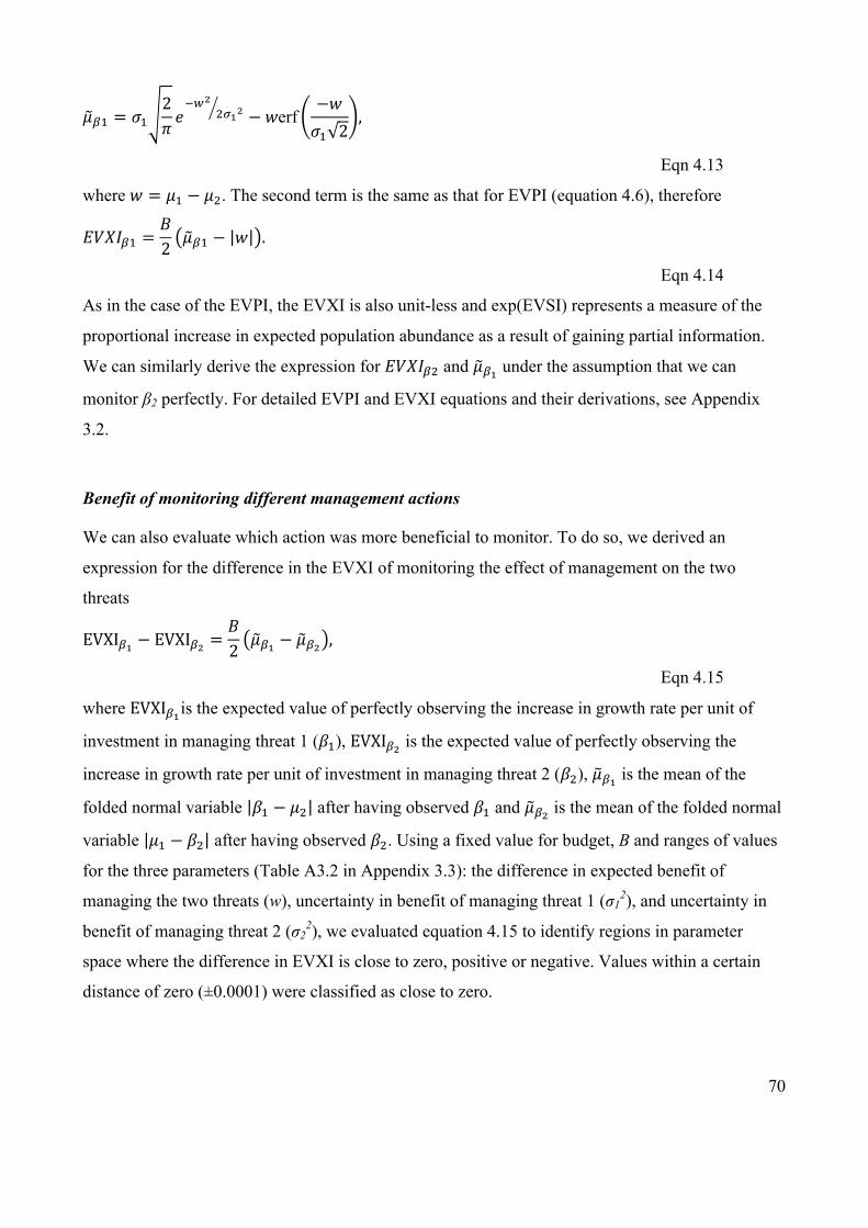
70

dW1 = e12

gUhiX

2oEX − kerf−k

e1 2,

Eqn 4.13

where k = d1 − d2. The second term is the same as that for EVPI (equation 4.6), therefore

>?l@W1 =5

2dW1 − k .

Eqn 4.14

As in the case of the EVPI, the EVXI is also unit-less and exp(EVSI) represents a measure of the

proportional increase in expected population abundance as a result of gaining partial information.

We can similarly derive the expression for >?l@W2 and dWE under the assumption that we can

monitor β2 perfectly. For detailed EVPI and EVXI equations and their derivations, see Appendix

3.2.

Benefit of monitoring different management actions

We can also evaluate which action was more beneficial to monitor. To do so, we derived an

expression for the difference in the EVXI of monitoring the effect of management on the two

threats

EVXIWE − EVXIWX =5

2dWE − dWX ,

Eqn 4.15

where EVXIWEis the expected value of perfectly observing the increase in growth rate per unit of

investment in managing threat 1 (Z1), EVXIWX is the expected value of perfectly observing the

increase in growth rate per unit of investment in managing threat 2 (Z2), dWE is the mean of the

folded normal variable Z1 − d2 after having observed Z1 and dWX is the mean of the folded normal

variable d1 − Z2 after having observed Z2. Using a fixed value for budget, B and ranges of values

for the three parameters (Table A3.2 in Appendix 3.3): the difference in expected benefit of

managing the two threats (w), uncertainty in benefit of managing threat 1 (σ12), and uncertainty in

benefit of managing threat 2 (σ22), we evaluated equation 4.15 to identify regions in parameter

space where the difference in EVXI is close to zero, positive or negative. Values within a certain

distance of zero (±0.0001) were classified as close to zero.

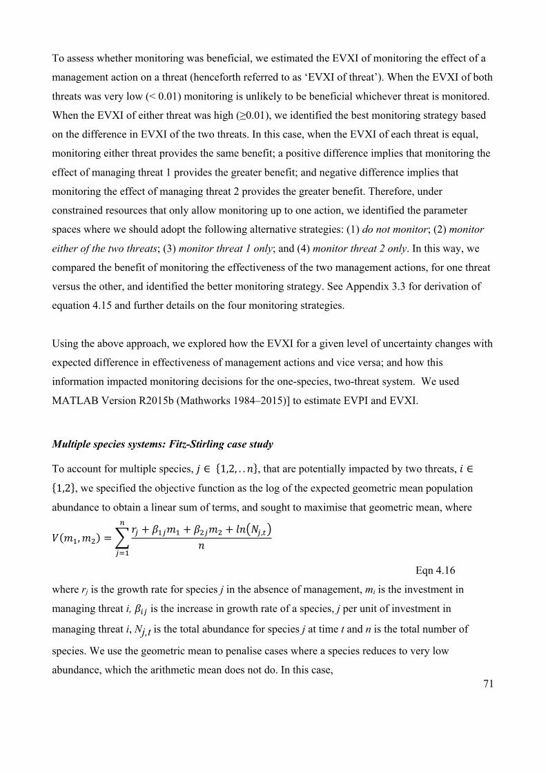
71

To assess whether monitoring was beneficial, we estimated the EVXI of monitoring the effect of a

management action on a threat (henceforth referred to as ‘EVXI of threat’). When the EVXI of both

threats was very low (< 0.01) monitoring is unlikely to be beneficial whichever threat is monitored.

When the EVXI of either threat was high (≥0.01), we identified the best monitoring strategy based

on the difference in EVXI of the two threats. In this case, when the EVXI of each threat is equal,

monitoring either threat provides the same benefit; a positive difference implies that monitoring the

effect of managing threat 1 provides the greater benefit; and negative difference implies that

monitoring the effect of managing threat 2 provides the greater benefit. Therefore, under

constrained resources that only allow monitoring up to one action, we identified the parameter

spaces where we should adopt the following alternative strategies: (1) do not monitor; (2) monitor

either of the two threats; (3) monitor threat 1 only; and (4) monitor threat 2 only. In this way, we

compared the benefit of monitoring the effectiveness of the two management actions, for one threat

versus the other, and identified the better monitoring strategy. See Appendix 3.3 for derivation of

equation 4.15 and further details on the four monitoring strategies.

Using the above approach, we explored how the EVXI for a given level of uncertainty changes with

expected difference in effectiveness of management actions and vice versa; and how this

information impacted monitoring decisions for the one-species, two-threat system. We used

MATLAB Version R2015b (Mathworks 1984–2015)] to estimate EVPI and EVXI.

Multiple species systems: Fitz-Stirling case study

To account for multiple species, ! ∈ 1,2, . . \ , that are potentially impacted by two threats, ( ∈

1,2 , we specified the objective function as the log of the expected geometric mean population

abundance to obtain a linear sum of terms, and sought to maximise that geometric mean, where

? 41,42 =P+ + Z1+41 + Z2+42 + [\ Q+,R

\

q

+<1

Eqn 4.16

where rj is the growth rate for species j in the absence of management, mi is the investment in

managing threat i, Z*+ is the increase in growth rate of a species, j per unit of investment in

managing threat i, Nj,t is the total abundance for species j at time t and n is the total number of

species. We use the geometric mean to penalise cases where a species reduces to very low

abundance, which the arithmetic mean does not do. In this case,

72

>?-@ = r

2qd − k and

Eqn 4.17

d =2 e1

2 + e22

gUh

sEhsXX

2 oEXSoX

X− d1 − d2 UPF

− d1 − d2

2 e12 + e2

2

Eqn 4.18

where µ1 and µ2 are prior expected benefit of managing threat 1 and threat 2 for all n species,

respectively; σ12 and σ2

2 are the uncertainties in benefit of managing threat 1 and threat 2 for all n

species, respectively. w represents the difference in expected effectiveness of managing threat 1 and

2 for all n species. The value of monitoring β1 perfectly, i.e. monitoring the effect of managing

threat 1 on the species, can be expressed as

>?l@W1 = 5

2\dW1 − k

Eqn 4.19

where

dW1 =2 e1

2

gUh sEhsX

X

2 oEX− d1 − d2 UPF

− d1 − d2

2 e12

Eqn 4.20

and here, exp(EVXI) is a measure of the proportional increase in the expected geometric mean

population abundance of species ! ∈ 1,2, . . \ and is unit-less. Here, it represents a measure of the

proportional increase in the geometric mean of abundances. Appendix 3.4 provides detailed EVPI

and EVXI equations for the n-species, 2-threat system. Additionally, Appendix 3.5 provides the

formulation for monitoring the effect of management on growth rates of a subset of the species in

the n-species, 2-threat system to represent more realistic decision scenarios.

Our case study was based in Western Australia, in an internationally recognised global biodiversity

hotspot, the Fitz-Stirling – fragmented remnant patches of woodland and heathland in agricultural

land stretching 70km from the Stirling Ranges to Fitzgerald River National Parks in southwestern

Australia. We considered three target species: Trichosurus vulpecula (western brushtail possum),

Macropus eugenii (tammar wallaby) and Isoodon obesulus (southern brown bandicoot or quenda),

under two key threats: the invasive predator, Vulpes vulpes (European red fox) and altered fire

regimes. Management strategies for recovering mammals in several large protected areas in the

region involve poison baiting for foxes, and active fire management to prevent too-frequent fires

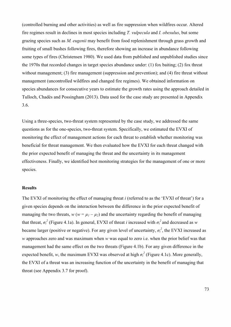
73

(controlled burning and other activities) as well as fire suppression when wildfires occur. Altered

fire regimes result in declines in most species including T. vulpecula and I. obesulus, but some

grazing species such as M. eugenii may benefit from food replenishment through grass growth and

fruiting of small bushes following fires, therefore showing an increase in abundance following

some types of fires (Christensen 1980). We used data from published and unpublished studies since

the 1970s that recorded changes in target species abundance under: (1) fox baiting; (2) fox threat

without management; (3) fire management (suppression and prevention); and (4) fire threat without

management (uncontrolled wildfires and changed fire regimes). We obtained information on

species abundances for consecutive years to estimate the growth rates using the approach detailed in

Tulloch, Chadès and Possingham (2013). Data used for the case study are presented in Appendix

3.6.

Using a three-species, two-threat system represented by the case study, we addressed the same

questions as for the one-species, two-threat system. Specifically, we estimated the EVXI of

monitoring the effect of management actions for each threat to establish whether monitoring was

beneficial for threat management. We then evaluated how the EVXI for each threat changed with

the prior expected benefit of managing the threat and the uncertainty in its management

effectiveness. Finally, we identified best monitoring strategies for the management of one or more

species.

Results

The EVXI of monitoring the effect of managing threat i (referred to as the ‘EVXI of threat’) for a

given species depends on the interaction between the difference in the prior expected benefit of

managing the two threats, w (w = µ1 – µ2) and the uncertainty regarding the benefit of managing

that threat, σi2 (Figure 4.1a). In general, EVXI of threat i increased with σi

2 and decreased as w

became larger (positive or negative). For any given level of uncertainty, σi2, the EVXI increased as

w approaches zero and was maximum when w was equal to zero i.e. when the prior belief was that

management had the same effect on the two threats (Figure 4.1b). For any given difference in the

expected benefit, w, the maximum EVXI was observed at high σi2 (Figure 4.1c). More generally,

the EVXI of a threat was an increasing function of the uncertainty in the benefit of managing that

threat (see Appendix 3.7 for proof).

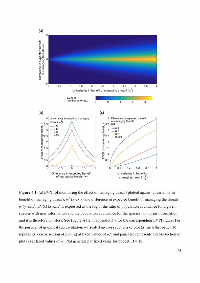
74

Figure 4.1: (a) EVXI of monitoring the effect of managing threat i plotted against uncertainty in

benefit of managing threat i, σi2 (x-axis) and difference in expected benefit of managing the threats,

w (y-axis). EVXI (z-axis) is expressed as the log of the ratio of population abundance for a given

species with new information and the population abundance for the species with prior information;

and it is therefore unit-less. See Figure A3.2 in appendix 3.8 for the corresponding EVPI figure. For

the purpose of graphical representation, we scaled up cross sections of plot (a) such that panel (b)

represents a cross section of plot (a) at fixed values of σi2; and panel (c) represents a cross section of

plot (a) at fixed values of w. Plot generated at fixed value for budget, B = 10.

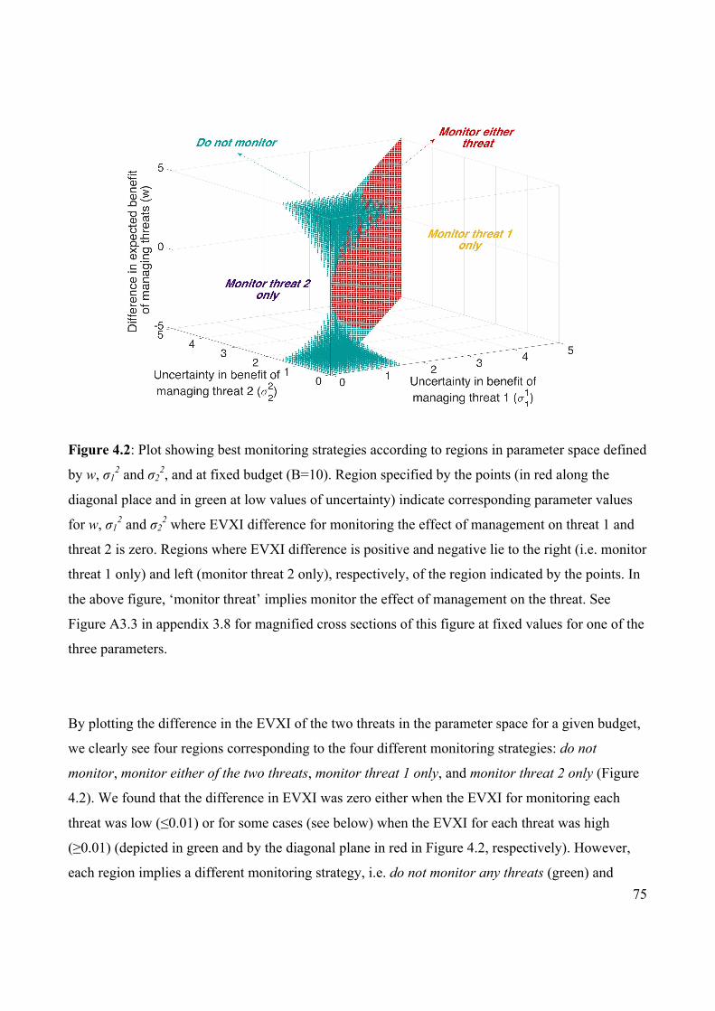
75

Figure 4.2: Plot showing best monitoring strategies according to regions in parameter space defined

by w, σ12 and σ2

2, and at fixed budget (B=10). Region specified by the points (in red along the

diagonal place and in green at low values of uncertainty) indicate corresponding parameter values

for w, σ12 and σ2

2 where EVXI difference for monitoring the effect of management on threat 1 and

threat 2 is zero. Regions where EVXI difference is positive and negative lie to the right (i.e. monitor

threat 1 only) and left (monitor threat 2 only), respectively, of the region indicated by the points. In

the above figure, ‘monitor threat’ implies monitor the effect of management on the threat. See

Figure A3.3 in appendix 3.8 for magnified cross sections of this figure at fixed values for one of the

three parameters.

By plotting the difference in the EVXI of the two threats in the parameter space for a given budget,

we clearly see four regions corresponding to the four different monitoring strategies: do not

monitor, monitor either of the two threats, monitor threat 1 only, and monitor threat 2 only (Figure

4.2). We found that the difference in EVXI was zero either when the EVXI for monitoring each

threat was low (≤0.01) or for some cases (see below) when the EVXI for each threat was high

(≥0.01) (depicted in green and by the diagonal plane in red in Figure 4.2, respectively). However,

each region implies a different monitoring strategy, i.e. do not monitor any threats (green) and

76

monitor either of the two threats (red). The former strategy (do not monitor) was selected when the

difference in the expected benefit of managing threats was large and the uncertainty in benefit of

management for each threat was small. The latter strategy (monitor either threat) was selected when

the uncertainties in the benefit of managing threat 1 and threat 2 were equal. The EVXI for each

threat was also high (≥0.01) outside of these regions. Here, the monitor threat 1 only strategy was

selected when the difference in EVXI was positive. This implied that the uncertainty in the benefit

of managing threat 1 was greater than that for threat 2; therefore monitoring threat 1 provided

greater benefit for management. Conversely, the monitor threat 2 only strategy was selected when

uncertainty in the benefit of managing threat 2 was greater than that for threat 1.

When considering multiple species as in the Fitz-Stirling case study, the choice of the best

monitoring strategy follows the general trends described above, but changes with the species

considered in the decision problem (Figure 4.3). When only considering one species, M. eugenii,

the EVXI for fire management was higher than that for fox management, however the overall

benefit of monitoring to evaluate management effectiveness for either threat was low for this

species. In contrast, EVXI for fox management was higher than that for fire management in the case

of I. obesulus or T. vulpecula. When considering pairs of species, the EVXI of fire management

was marginally higher than that for fox management for pairs including M. eugenii, however, as

seen before, EVXI across the threats was low for these pairs. Again, the EVXI for fox management

was higher when considering I. obesulus and T. vulpecula together. When considering all three

species, EVXI across threats was low and EVXI for fire management was higher compared to that

for fox management. These results were also illustrated by plotting the species in the parameter

space defined by w, σ12 and σ2

2 (Figure 4.4). Point estimates for the difference in the expected

benefit of managing the two threats, w, for I. obesulus as well as for T. vulpecula were close to the

boundary, defined by equal uncertainty in management effectiveness for each threat, beyond which

the selected monitoring strategy switches, i.e. from ‘monitor foxes only’ to ‘monitor fire only’

(Figures 4.4a and 4.4b, respectively). On the other hand, point estimates for w for M. eugenii and

when considering all three species together, is located away from the boundaries representing a

switch in monitoring strategies (Figures 4.4c and 4.4d, respectively).

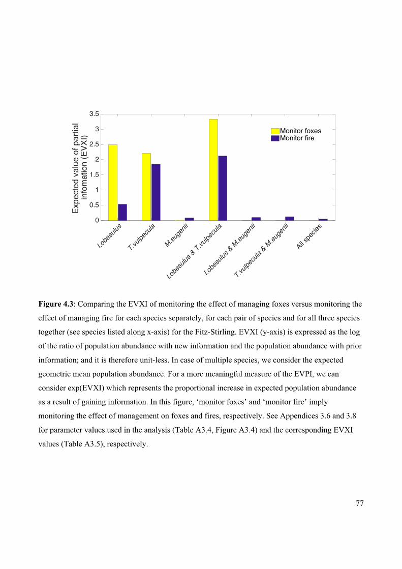
77

Figure 4.3: Comparing the EVXI of monitoring the effect of managing foxes versus monitoring the

effect of managing fire for each species separately, for each pair of species and for all three species

together (see species listed along x-axis) for the Fitz-Stirling. EVXI (y-axis) is expressed as the log

of the ratio of population abundance with new information and the population abundance with prior

information; and it is therefore unit-less. In case of multiple species, we consider the expected

geometric mean population abundance. For a more meaningful measure of the EVPI, we can

consider exp(EVXI) which represents the proportional increase in expected population abundance

as a result of gaining information. In this figure, ‘monitor foxes’ and ‘monitor fire’ imply

monitoring the effect of management on foxes and fires, respectively. See Appendices 3.6 and 3.8

for parameter values used in the analysis (Table A3.4, Figure A3.4) and the corresponding EVXI

values (Table A3.5), respectively.

I.obe

sulus

T.vulpe

cula

M.euge

nii

I.obe

sulus

& T.vulpe

cula

I.obe

sulus

& M.eu

genii

T.vulpe

cula

& M.eu

genii

All spe

cies

0

0.5

1

1.5

2

2.5

3

3.5

Expe

cted

val

ue o

f par

tial

info

mat

ion

(EVX

I)

Monitor foxesMonitor fire

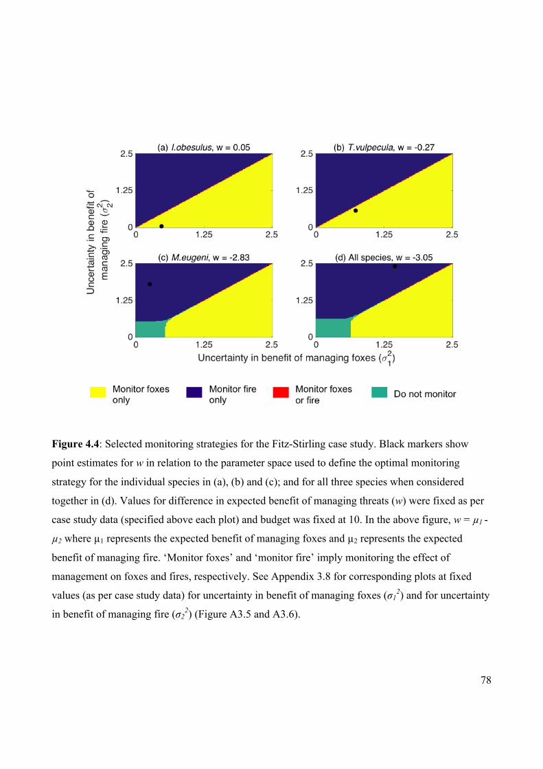
78

Figure 4.4: Selected monitoring strategies for the Fitz-Stirling case study. Black markers show

point estimates for w in relation to the parameter space used to define the optimal monitoring

strategy for the individual species in (a), (b) and (c); and for all three species when considered

together in (d). Values for difference in expected benefit of managing threats (w) were fixed as per

case study data (specified above each plot) and budget was fixed at 10. In the above figure, w = µ1 -

µ2 where µ1 represents the expected benefit of managing foxes and µ2 represents the expected

benefit of managing fire. ‘Monitor foxes’ and ‘monitor fire’ imply monitoring the effect of

management on foxes and fires, respectively. See Appendix 3.8 for corresponding plots at fixed

values (as per case study data) for uncertainty in benefit of managing foxes (σ12) and for uncertainty

in benefit of managing fire (σ22) (Figure A3.5 and A3.6).

79

Discussion

Managers usually have some prior knowledge regarding the effectiveness of alternative threat

management actions (e.g. an expected change in growth rate of a species due to mitigation of a

threat), but this information is often uncertain (Evans, Possingham & Wilson 2011). Here, we

demonstrate the use of VOI analysis to identify monitoring strategies that inform decisions about

multiple threat management strategies when knowledge regarding the effectiveness of management

actions is uncertain. We find that, for a given threat, the value of monitoring to inform management

(i.e. whether to monitor threat mitigation or not) depends on the difference in the prior expected

benefit of managing the two threats and the uncertainty in the benefit of managing the threat.

Importantly, in cases where monitoring is found to be beneficial, the choice of the best monitoring

strategy to depends only on the uncertainty in the benefit of managing the threats.

In a one-species, two-threat system, the value of monitoring to learn about the effect of managing a

threat (EVXI) is determined by the uncertainty in management effectiveness and the difference in

the management effectiveness for the two threats (Figure 4.1). Interestingly, uncertainty in growth

rate of species in the absence of management does not affect the EVXI because it drops out of the

VOI equations (see equations 4.10 and 4.14). As expected, EVXI increases with the uncertainty in

the effect of management on that threat (Appendix 3.7). However, the influence of uncertainty on

the EVXI varies according to the prior knowledge on the difference in management effectiveness

for the two threats. Specifically, uncertainty has a stronger influence on the value of monitoring (i.e.

leads to higher EVXI) when management actions for each threat result in similar changes in the

growth rates of the target species, as compared to when actions have significantly different effects

on the growth rates. It therefore follows that the EVXI is highest when both actions have a similar

effect on species’ growth rate. This is because, in these cases, we are less certain about which

management action is more likely to change the growth rate of the species; and so we are unsure of

which threat to manage. For example, in our three-species two-threat system, given differences in

the relative uncertainty in the effect of managing foxes (σi2 = 0.4675 for I. obesulus and σi

2 = 0.2543

for M. eugenii), EVXI for fox management is higher for I. obesulus (EVXI = 2.4868) than for M.

eugenii (EVXI = 0). This is because the expected prior benefit of managing foxes and fire for I.

obesulus is similar (1.0729 and 1.0233, respectively) compared to M. eugenii (0.9476 and 3.7752,

respectively). The EVXI for I. obesulus for fox management (EVXI = 2.4868) can be interpreted in

80

terms of its exponential i.e. proportional increase of 12 in expected population abundance as a result

of gaining information.

In some situations managers may choose not to implement any monitoring, thereby averting the risk

of wasting time, effort and resources when monitoring is not warranted for decision-making

(McDonald-Madden et al. 2010a). For managing multiple threats, we found this to be the case when

the difference in the prior expected benefit of managing threats was large and the uncertainty in

benefit of management for each threat was small (Figure 4.2). This is because, in these situations,

the decision regarding which action to implement (i.e. which threat to manage) is intuitive and the

manager should choose the action that leads to better management outcomes based on prior

knowledge. For cases where monitoring is found to be beneficial for management decision-making

(i.e. EVXI for each threat ≥0.01), the choice of best monitoring strategy to learn about management

effectiveness is determined only by the uncertainty in the benefit of alternate threat management

actions (Figure 4.2). When we are equally uncertain about the effect of management on the two

threats, the choice of the strategy is not important as we can monitor either (see Appendix 3.3).

However, when the uncertainty in the effect of management on the two threats is unequal,

monitoring the effect of management on the threat with the greater uncertainty always provides

higher benefit. This implies that monitoring need not always target threats and management actions

with the highest perceived impacts on biodiversity.

The general patterns of which threat to monitor when uncertainty in management effectiveness

varies are clearly demonstrated by the case study when considering one, two or three species for

management (Figure 4.3). In the case of I. obesulus or T. vulpecula, EVXI of fox management is

higher than the EVXI for managing fire because, while both management actions have similar

expected benefits for the species (Figure A3.4), uncertainty in management effectiveness for foxes

is higher than that for fire. In contrast, for M. eugenii, monitoring fire management provides higher

benefit as opposed to monitoring fox management (EVXI = 0), because uncertainty in the benefit of

managing fire is much higher than that of managing foxes. Additionally, M. eugenii exhibits large

differences between the two threats in the expected benefit of their management. There is little

value of monitoring (EVXI) to learn about management effectiveness for this species, as the

dominant threatening process (fox predation) is understood and can be targeted immediately. This

indicates that for I. obesulus or T. vulpecula, the optimal strategy of monitoring foxes results in a

81

greater proportional increase in its abundance as opposed to monitoring fire. Alternately, M. eugenii

benefits instead from fire monitoring instead.

When considering more than one species in making a decision about which threat management

action to monitor, we aggregate the expected benefits and the uncertainty across species (see

Appendix 3.4). In our case study, because the effect of management and uncertainty for M. eugenii

is highly skewed towards one threat rather than the other, this species heavily influences the results,

leading to larger differences in expected benefit and higher aggregated uncertainty regarding

management of fire (Figures A3.4 and 4.3). This leads to the low value of monitoring (EVXI) and

the selection of monitoring to learn about the effect of management on fire as the optimal strategy

for combinations of species including M. eugenii. Finally, the locations of the point estimates for

the difference in the expected benefit of managing the two threats, w, specified according to the

species in Figure 4.4 indicate whether the chosen monitoring strategy for the species is robust to

uncertainty in w. For instance, uncertainty in w would likely change the decision of the best

monitoring strategy for T. vulpecula and to a lesser extent for I. obesulus as these points lie closer to

the boundary across which the selected monitoring strategy switches. The same results are seen for

T. vulpecula and I. obesulus when considering uncertainty in the point estimates for σ12 and σ2

2

(Figures A3.5 and A3.6, respectively). However, the sensitivity of the selected monitoring strategy

to uncertainty in parameter estimates needs to be evaluated quantitatively.

For the Fitz-Stirling case study, two species, I. obesulus and T. vulpecula provide the greatest

benefit when monitored for the effect of management in this chapter and under the experimental

strategy in chapter three. However, the selected monitoring strategies vary between the two

chapters: monitoring to learn the effect of management of foxes (this chapter) versus experimentally

managing fire to learn about the impact of fire (chapter three). The difference in the selection of the

optimal monitoring strategy is not straightforward to explain because the questions asked and the

VOI formulation used in the two chapters differs markedly. In chapter three, we wanted to assess

how VOI and the choice of the best monitoring strategy change with the parameters of the decision

problem including the budget available for management, prior understanding of whether threats

cause declines, and the relative cost of managing these threats. We considered threats to either

cause a decline in a species or not, and the uncertainty in the decision problem was regarding

whether species were declining and if so, which threats caused declines in which species. To apply

the VOI approach, we assigned probabilities of decline and no decline for each species due to each

82

threat and its management and evaluated the benefit of monitoring different species by varying the

parameters of the decision problem. In contrast, in this study we asked how VOI and choice of the

best monitoring strategy change with prior knowledge of management effectiveness and the

uncertainty regarding the effectiveness. The approach presented here allows us to address

conservation decisions informed by the magnitude of impact of threat management activities, which

was not considered in chapter three. To do so, we used a stochastic model of exponential population

growth to allow modelling the effect of management of a threat as the change in growth rate of

species under alternative threat management actions and uncertainty as the variance in the growth

rate estimate. Moreover, we did not consider the influence of varying budget or costs of

management in this study.

The distinction in the VOI formulation used in the two chapters is important to enable the selection

of the appropriate monitoring and management strategies. The approach presented in this chapter is

useful when managers have some information regarding the effectiveness of their management

actions. Information regarding change in species growth rate under threats and their management

can be obtained from published studies, management reports or monitoring data (e.g. Tulloch,

Chadès & Possingham 2013; U.S. Fish and Wildlife Service 2015); or the information may

obtained based on past experience as in the case of adaptive management or information exchange

amongst managers faced with similar decisions but at different spatial locations (Cook et al. 2012).

However, a number of conservation problems lack even a basic understanding of the threats and/or

species present in the system, and the impacts of threats and their management (Cook, Hockings &

Carter 2010). Expert elicitation can help obtain preliminary information regarding threats and their

probable impacts in the absence of empirical evidence (Carwardine et al. 2012; Martin et al.

2012a). In these cases the VOI approach presented in chapter three that considers probability of

impact rather than the magnitude of impact of threats and their management, would prove more

useful. Finally, increasing the number of species in the VOI formulation in chapter three made the

approach computationally challenging as it significantly increased the number of decision

parameters that needed to be considered in the optimisation. However, managers are usually faced

with decisions that include larger number of threats and species and the approach presented in this

chapter can be easily extended to consider larger systems (Appendix 3.4), though this could not be

demonstrated with the data available for the case study.

83

We made a number of assumptions in this study. Firstly, we assumed a linear relationship between

investment in managing a threat and the gain from managing the threat. This assumption may hold

over small parameter space, for instance when working under small management budgets for

localised management actions. However, over larger management budgets, we would expect that

investment in managing threats beyond a certain threshold would provide diminishing returns

(Wilson et al. 2006; Murdoch et al. 2007). Assuming a threshold function such that the benefit

peaks once the threshold is reached or a concave function to reflect diminishing returns (Teeffelen

& Moilanen 2008; Wilson, Carwardine & Possingham 2009) would provide some straightforward

ways to deal with this issue. Secondly, we considered the cost of monitoring implicitly by limiting

monitoring to one action only. However, there may be monetary costs of implementing monitoring

as well as opportunity costs when resources allocated for monitoring could have been used for

direct management actions (Cleary 2006; Grantham et al. 2008; McDonald-Madden et al. 2010a).

To ensure that monitoring decisions are cost-effective, the benefits of resolving uncertainty in

decision making need to be traded-off against the costs of monitoring as this has been shown to

influence VOI and the selection of optimal monitoring strategies for decision-making (Field et al.

2004; Maxwell et al. 2015). Additionally, development of efficient and effective monitoring

strategies for complex systems under conditions of management (financial) constraints requires that

the trade-offs in budgeting for threats management and multi-species monitoring be assessed. As

already discussed in chapter three, the adaptive management literature can provide guidance on how

to address this issue.

Finally, we assume perfect detection of the effect of management on species growth rates through a

given monitoring action. This is rarely the case, as there are usually different monitoring actions

available even for the same species-threat combination (e.g. direct capture-mark-recapture versus

distance sampling methods), each of which may provide different (and sometimes complementary)

information (e.g. population process data versus population abundance data) (Regan, Chadès &

Possingham 2011; Nichols 2006). Despite this, such simplifications are a necessary first step to

establish a basic understanding of decision-making for complex multi-threat systems, and to

subsequently infer the consequences of incorporating observation errors into the decision model.

One solution is to use the expected value of sample information (EVSI), which measures the

expected improvement in outcomes from acquiring imperfect information from monitoring (see

chapter three). Alternatively (or additionally), future research could employ probability

distributions for the uncertain parameters in the VOI formulation, or use partially observable

84

Markov decision processes that look for optimal solutions using observation probabilities and allow

dynamic updating of the probabilities over time (Chadès et al. 2008; Littman 2009; McDonald-

Madden et al. 2011). Moreover, optimal management decisions depend not only on the ability to

correctly detect system states or trends (Field et al. 2005; Wilson, Rhodes & Possingham 2015) but

also on understanding the impact of the threat (i.e. structural uncertainty; Williams 2001). We

assumed that the population model is true (management of threats has a linear effect on the

probability of species decline) and that this model structure is perfectly known but that there is

uncertainty in the parameters (i.e. the effects of management of threats on growth rate). As such,

structural uncertainty is ignored in this chapter but is a potential future direction.

In the context of management, monitoring has three basic roles: identifying the state of the system

for state-dependent decision-making, assessing effectiveness of management actions, and reducing

uncertainty about how the system functions to improve management decisions in the future (Lyons

et al. 2008). The VOI approach presented in this study provides valuable insights regarding when

monitoring to learn about management effectiveness is likely to be of value to inform management

of multiple threats and what the value of monitoring depends on. Furthermore, it allowed us to

examine how uncertainty in prior knowledge regarding management effectiveness can influence

management and monitoring decisions. In the face of multiple threats leading to biodiversity

decline and limited resources to manage these threats, such approaches will foster more reliable

monitoring decisions to inform and improve biodiversity conservation.

Acknowledgements


Environmental Decisions, a School Research Grant from the School of Geography, Planning and

Environmental Management at the University of Queensland and a University of Queensland

International Scholarship. We thank Ayesha Tulloch for providing data for the case study.

85

Cost-effective monitoring to trigger

conservation interventions

Prepared for submission to Methods in Ecology and Evolution

86

Chapter five – Cost-effective monitoring to trigger conservation

interventions

Abstract

Effective biodiversity conservation requires responding to threats in a timely fashion. This entails

an understanding of the impacts of threats to biodiversity and when interventions should be

implemented. However, most ecological systems face multiple threats and monitoring to assess

their impacts on biodiversity is a complex task. Indicators can help simplify the challenge of

monitoring multiple threats but choosing the best indicator(s) to monitor is not straightforward. As

resources for monitoring are limited, indicators need to be selected carefully to avoid inefficient or

ineffective management choices. We provide a decision framework for analyzing the cost-

effectiveness of indicators that can act as triggers for initiating management interventions in multi-

threat systems. Our framework utilises information on the threat impacts, sensitivity of indicators to

threats, and the benefits, costs and feasibility of monitoring alternative indicators to make informed

indicator choices for monitoring and managing multiple threats. Although similar indicator

selection criteria have been proposed in the literature, ours is the first approach to integrate multiple

selection criteria in a quantitative economic assessment of competing indicator choices. Using a

case study from Kimberley (Western Australia), we evaluate eighteen indicators for informing

management of three threats. We show that indicator selection based on our approach can help

improve threat management decisions when resources are limited, leading to better conservation

outcomes. Because our framework accounts for multiple criteria and accounts for the benefit of

monitoring the indicator with regard to the expected decision outcome, it improves on common

approaches whereby indicators may often be selected based only on whether they are sensitive to

change or cheap to monitor.

87

Introduction

Monitoring is an important element in the conservation of threatened biodiversity; whether to

demonstrate outcomes, raise awareness, learn about complex environments, or to trigger

management interventions (Nichols & Williams 2006; McDonald-Madden et al. 2010a;

Possingham et al. 2012). A significant focus of the ecological monitoring literature has been on the

role of indicators to detect change in ecological systems and inform conservation decisions (e.g.

Gregory et al. 2005; Blanchard et al. 2010; Caro 2010). Numerous conservation efforts rely on

indicators for monitoring when dealing with broad objectives for management such as restoring an

ecosystem (Lindenmayer, Margules & Botkin 2000; Lindenmayer & Likens 2011). Indicators are

proxies for ecological elements, processes, or properties too difficult to measure directly due to

logistical, financial, or technological reasons (Landres et al., 1988). While their use in conservation

has drawn mixed reviews (Carignan & Villard 2002; Seddon & Leech 2008; Fleishman & Murphy

2009), their practical utility has made them almost standard monitoring practice in ecological

systems (Caro 2010; Siddig et al. 2016). However, monitoring generally comes at a cost and

different indicators not only bear different monetary costs, but also different opportunity costs when

monitoring diverts resources from direct management action (McDonald-Madden et al. 2010a).

Moreover, alternative indicators may provide information capable of changing the course of

management decisions in different ways (see chapter three). Given current limitations in resources

available to conserve biodiversity (McCarthy et al. 2012), selecting appropriate indicators for

management decision-making therefore requires an explicit evaluation of the management

outcomes of monitoring alternate indicators and the associated costs of monitoring. The literature

on how to select cost-effective indicators for management decision-making is surprisingly sparse

and the aim of this study is to fill this gap.

A variety of approaches have been used to select indicators for monitoring (Carignan & Villard

2002). These range from the selection of species based on iconic status (Simberloff 1998;

Andelman & Fagan 2000; see chapter two) and the selection of biophysical characteristics

correlated to changes in the landscape (Lindenmayer et al. 2002), to approaches that incorporate a

complex set of considerations, such as feasibility, communicability and appropriateness of the

indicator for representing the system of concern (e.g. Pannell & Glenn 2000; Bossel 2001;

Niemeijer & de Groot 2008; Smyth et al. 2009; Heink & Kowarik 2010b). Despite the recognised

lack of funding for conservation endeavors, few approaches for selecting indicators explicitly

88

consider the costs, focusing instead on an indicator’s ability to represent the system of concern (but

see Tulloch, Possingham & Wilson 2011; Peck et al. 2014). Furthermore, few consider the

management benefits of monitoring indicators, which should be related to the choice of altering

management interventions and improving management outcomes (see Pannell & Glenn 2000; Peck

et al. 2014; Bal et al. in review).

An additional complication to choosing appropriate indicators for decision-making comes from the

fact that nearly all ecosystems face multiple threats. For example, coastal development, pollution,

overfishing and rises in sea temperatures due to climatic shifts, all threaten coral reef systems

(Hughes, Huang & Young 2013). Similarly, fire, invasive species and overgrazing threaten

terrestrial vertebrates in the north-west of Australia (Carwardine et al. 2012). When indicators need

to inform on the impact of multiple threats and trigger the relevant management interventions,

monitoring decisions are fraught with uncertainty, complexity and tradeoffs between indicator

choices. In such situations, managers need systematic methods to choose indicators that can inform

on the status of multiple threats and when interventions to mitigate the effect of threats on

biodiversity are most needed (Caro 2010). This requires explicit consideration of the management

context as well as the economic constraints for choosing the best indicators (see chapter two). These

complex decisions involve multiple criteria, and it is precisely in such situations that a systematic

approach to decision-making is most needed (Possingham et al. 2001).

We propose that informed decision-making for selecting indicators to monitor multiple threats

requires consideration of six factors:

1. The potential threats operating in the system, and the possible indicators of these threats

2. For each threat, the prior belief that its impact on biodiversity is significant enough to

trigger a management intervention

3. The best monitoring strategy for each indicator, and how feasible and costly is it

4. Whether the indicator can detect the level of change required to trigger a chosen

management intervention

5. The feasibility of the management intervention taken in response to the threat

6. The potential benefit from threat abatement

While decision makers are often aware of these factors, a straightforward method to combine these

factors is required to enable cost-effective decisions about which indicators to monitor to inform

89

management. Cost-effectiveness analysis (CE analysis) is a type of economic analysis to compare

the relative outcomes of alternate actions while accounting for the associated cost of

implementation (Laycock et al. 2009). It differs from traditional cost-benefit analysis in that the

outcomes of decisions (in this case the net management benefit of monitoring an indicator) do not

need to be monetized. CE analysis can explicitly incorporate financial considerations while

avoiding the ethical and practical dilemmas associated with putting a monetary value on species or

ecosystems, making it a useful method to support biodiversity conservation decision making

(Laycock et al. 2009). The approach has previously been used to prioritise threatened species

recovery projects (Cullen, Moran & Hughey 2005; Joseph, Maloney & Possingham 2008; Briggs

2009; Laycock et al. 2009), actions to mitigate threats to biodiversity (Carwardine et al. 2012; Firn

et al. 2015), landscape-scale environmental projects (Pannell et al. 2012), and spatial allocation of

conservation efforts (Polasky et al. 2005; Wilson et al. 2006; Auerbach, Tulloch & Possingham

2014). However, its application to prioritising monitoring actions is limited (but see Tulloch,

Possingham & Wilson 2011; Tulloch, Chadès & Possingham 2013) and to our knowledge it has

never been used for selecting indicators to inform management of multiple threats.

In this study, we provide a CE analysis framework to allow prioritisation of monitoring actions for

improving management outcomes in multi-threat systems. Specifically, we focus on how to

combine each of the six factors in an analysis for selecting indicators to trigger management

interventions for multiple threats. To demonstrate its application to real-world conservation

decisions, we apply our approach to a case study for monitoring and management of threats to the

terrestrial biota in the Kimberley region of northwest Australia. We also test the sensitivity of the

selection for the case study to uncertainty related to the six factors outlined above.

Methods

In the following sections we explain the CE analysis framework and detail the six factors

considered in this analysis. We then describe the case study application and describe how the

sensitivity analysis was conducted.


We consider a system where a manager wants to maximise the persistence of threatened biota of an

ecosystem impacted by multiple threats (the management objective). This requires prioritising

90

management actions for mitigating the impacts of those threats that have a significant impact on the

biodiversity of the region. In order to inform her decisions, the manager needs to identify indicators

for monitoring that can tell her when management interventions are required for the different

threats. However, working with a limited budget, she wants to select the most cost-effective

indicators that can be used to trigger management interventions for mitigating the multiple threats.

Cost-effective analysis framework

An expression of the cost-effectiveness of an indicator for triggering management interventions for

multiple threats, comprises six main components: (1) a list of the potential threats operating in the

system and their possible indicators; (2) the prior probability of each threat having a significant

enough impact on biodiversity to trigger a management intervention; (3) the feasibility and the cost

of monitoring each indicator; (4) the probability that an indicator can detect the level of change in a

threat required to trigger a management intervention; (5) the probability that the management

intervention taken in response to the threat is feasible; and (6) the expected benefit from threat

abatement. In our analysis we assume that: a) a given indicator can inform on one or more threats;

b) for a given threat, there can be multiple indicators that could be used to detect whether the impact

of the threat triggers a management intervention; and c) for a given threat, there is one (or a suite

of) chosen management intervention(s).

These factors can be combined to derive an expression for the overall expected benefit of

monitoring an indicator, i, for the management of the multiple threats present in the system (Bi).

The logic for combining these factors is shown in Figure 5.1a, which shows how the expected

benefit of monitoring an indicator, i, for an individual threat, j can be expressed as

5* = t+u*)*+u+5++

.

Eqn 5.1

Here t+ represents the probability of threat j causing an impact of magnitude equivalent to a pre-

defined trigger point for implementing a chosen management intervention; u* is the probability that

monitoring indicator i is feasible; )*+ is the probability that monitoring indicator i can detect the

level of change required in threat j to trigger the management intervention; u+ is the probability that

91

the management intervention taken in response to threat j is feasible; and 5+ is the expected benefit

from implementing the management intervention for all species considered. Therefore, the benefit

of monitoring indicator i is represented in terms of the outcomes of the management intervention

for threat j.

Finally, as shown schematically in Figure 5.1b we specify the cost-effectiveness of indicator i as the

expected net benefit of monitoring that indicator across all threats relative to its cost of monitoring,

v* as

>* =5*v*.

Eqn 5.2

Indicators can then be ranked in decreasing order of cost-effectiveness (Joseph, Maloney &

Possingham 2008; Firn et al. 2015), with this ranking then used to make the final indicator

selection. One useful way to identify a cut-off point for the selection of multiple indicators is to

examine the marginal change in benefit as additional indicators are selected from the ranked list.

The point at which the marginal change in benefits with each added indicator diminishes below a

certain level can then be designated as the cut-off. We did this by plotting the cumulative benefits

against cumulative costs for each indicator in order of cost-effectiveness. We defined the point of

diminishing returns to be the point after which when adding an additional indicator resulted in less

than 20% change in the cumulative expected benefit relative to the cumulative cost of monitoring

an indicator, i.e.

ΔCumulative5*ΔCumulativev*

≤ 0.2.

Eqn 5.3

Our approach approximates optimal indicator(s) selection under a specified constraint (i.e. a

threshold for diminishing returns). A budget constraint could instead be specified as an alternative

to this method, such that indicators are selected until the budget allocated for monitoring is

exhausted.

92

Figure 5.1: (a) Schematic diagram of the how the factors combine for estimating the expected

benefit of monitoring an indicator, i, for an individual threat, j. Green nodes show how the expected

benefit is estimated in our cost-effectiveness framework. Red nodes, also known as ‘zero-benefit’

nodes, represent situations where probabilities of zero lead to no benefit from monitoring the

indicator. (b) Calculating cost-effectiveness of an indicator, i, as the expected net benefit of

monitoring an indicator across all threats relative to its cost of monitoring.

Probability*of*threat*j*affec0ng*the*system:"

Feasibility*of*the*best*monitoring*strategy*for*indicator*i:*

Probability*of*indicator*detec0ng*change*in*threat:*

Feasibility*of*best*interven0on*for*this*threat:*

Benefit*of*managing*this*threat:"

Expected*benefit*of*monitoring*indicator,*i,*for*threat,*j:"

Not*detect*(1Bpij)*

Detect*(pij)*

Feasible*(Fj)*

Not*feasible*(1BFj)*

Assets*protected*(Bj)*0* 0*

bj*Fi"pij"Fj"Bj""–* –* –* –*

Feasible*(Fi)*

Not*feasible*(1BFi)*

Probability*of*threat*(bj)*

Probability*of*no*threat*(1Bbj)*

0* 0*

(a)$

(b)$Benefit&of&monitoring&&indicator&for&threat&1&

Cost4effec6veness&&of&monitoring&indicator,&&i,&across&all&threats:&

Benefit:&&b2&Fi%pi2%F2%B2%%

+& +& +&…&Benefit:&&b3&Fi%pi3%F3%B3%%

Cost&of&monitoring&indicator,&i&

Benefit:&&b1&Fi%pi1%F1%B1%

Benefit&of&monitoring&&indicator&for&threat&2&

Benefit&of&monitoring&&indicator&for&threat&3&…&pij!

Fj!

1!

Bj!

Benefit*–! –! –! –!

Fi!

bj!

pij!

Fj!

1!

Bj!

Benefit*–! –! –! –!

Fi!

bj!

pij!

Fj!

1!

Bj!

Benefit*–! –! –! –!

Fi!

bj!

93

Table 5.1: Parameter notation used in the study

Parameter Notation

Indicator (index) (

Threat (index) !

Asset or species group (index) [

Number of species in an asset, l \}

Cost effectiveness of an indicator, i >*

Feasibility of monitoring an indicator, i u*

Benefit of monitoring an indicator, i 5*

Cost of monitoring an indicator, i v*

Prior belief in impact of a threat, j t+ Probability of an indicator, i, detecting enough change in threat, j, to trigger a chosen management intervention )*+

Feasibility of the chosen management intervention for threat, j u+ Benefit of the chosen management intervention for a threat, j (across all assets) 5+ Probability of persistence for asset, l, under no management for threat, j )}+

~ Probability of persistence for asset, l, under the chosen management intervention for threat, j )}+

Six factors for indicator selection

I. What potential threats are operating in the system and what are the possible indicators of

these threats?

Before we can decide which indicators we might monitor, we need to formulate a list of the

potential threats, j, which may be acting in a region. For each threat that is perceived to be acting on

the system currently or in the future, indicators of change, i, for this threat need to also be identified

based on some functional relationship between a state variable of that indicator and the impact of

the threat to the broader system.

94

II. For each threat, is the prior belief in its impact on biodiversity significant enough to trigger

a management intervention?

Decision triggers or trigger points to indicate when a system is moving to an undesirable state can

tell managers when to intervene to ensure conservation interventions are timely (Nichols, Eaton &

Martin 2014; Addison, de Bie & Rumpff 2015; Cook et al. 2016). These may be specified based on

long-term monitoring data using methods such as control charts (Morrison 2008) or on value-based

judgments (Martin et al. 2009) or using expert elicitation (Martin et al. 2012a). Fisheries,

agriculture and water quality management provide specific guidance regarding the process of

specifying triggers for management interventions over short time frames, for example for setting

threshold fishable biomass (McClanahan et al. 2011), fruit fly numbers in the horticulture industry

(Dominiak, Daniels & Mapson 2011) and contaminant concentrations in a river (ANZECC 2000).

When there are multiple threats impacting biodiversity, there can be variation in the magnitude of

threat impacts in space and in time. For indicator selection, incorporating the probability of threat j

causing an impact of magnitude equivalent to a pre-defined trigger point so as to trigger a chosen

management intervention, t+, will enable us to favour indicators of those threats believed a-priori to

have a significant impact in the region.

III. What is the best monitoring strategy for each indicator, and how feasible and costly is it?

It is essential to consider how best to monitor each indicator considered in the selection. Once an

optimal or best practice monitoring strategy for each potential indicator is identified, the costs of

monitoring the indicator and the probability that monitoring will be implemented can be

determined. We note that even if a best monitoring strategy is identified, there may be several

reasons it may not be implemented (e.g. budget constraints, or social, political or technical reasons)

(Field et al. 2007). For example, if activities such as bird banding face opposition from animal

rights activists (Şekercioğlu 2012) or monitoring techniques such as bioacoustics require specialised

skills and expertise (Dema et al. 2016; Zamora‐Gutierrez et al. 2016), they are likely to not be taken

up. On the other hand, monitoring of some indicators may have feasibility close to one because the

availability of well-established monitoring methods and expertise, e.g. koala monitoring using line

and strip transects (McGregor, Kerr & Krockenberger 2013). We capture this as the feasibility, u*,

which is the probability that the monitoring of an indicator actually happens. In order to generalise

the approach, we suggest eliciting relative values for the costs of monitoring the alternative

indicators, v*. This is because, unlike absolute costs, we expect the relative costs to remain fairly

constant if the approach is applied across different regions.

95

IV. Can the indicator detect the level of change required to trigger a chosen management

intervention?

The fundamental aim of monitoring is to ensure that real change is detected and acted upon as

promptly as possible (Legg & Nagy 2006; Field et al. 2007). When monitoring is intended to

conserve threatened species, indicators should aim to detect biodiversity changes in response to

threats that trigger specific and timely conservation actions (Lindenmayer, Piggott & Wintle 2013).

To fully evaluate the benefits of an indicator for triggering interventions across multiple threats, we

must ask for each indicator-threat combination ‘what is the probability that indicator, i, will detect a

sufficiently significant change in threat, j to enable a chosen management intervention to be

triggered in a timely manner?’ This probability, )*+, implies the monitoring regime/data/indicator

has adequate statistical power to enable informed decision-making (Field et al. 2004). Whether this

is the case may not be a straightforward question to answer. Eliciting this information from experts

requires an explicit definition of the level of change required to trigger management intervention

(trigger point) before the ability of the indicator to detect this level of change can be estimated

through the use of power analysis (Thomas 1997; Maxwell & Jennings 2005). When coming up

with the best monitoring strategy for a particular indicator it is likely that the power to detect a

change in that indicator has already been established, either through an explicit power analysis or

through some formal or informal expert knowledge. It is important to note that, there will always be

some probability of a Type II error (false negative) in whether the indicator will detect a sufficiently

significant change in threat (Mapstone 1995; Field et al. 2004). In this case, a Type II error would

result in the indicator failing to detect real change in the threat.

Although it is possible that a power analysis or expert opinion may already be established for

informing about the status of the indicator itself, it is unlikely that such a relationship will be

understood a-priori for the purposes of monitoring the status of the larger system. As such,

obtaining an explicit understanding of the level of change required to trigger management is a

difficult prospect. This is because such parameters are conditional on preceding events. For )*+for

example, the threat must have a significant impact, the significant level of threat impact must be

clearly specified and an action must be triggered given the change is detected. In such cases, visual

aids such as mental models to represent cause-and-effect dynamics can help step through the

information that needs to be elicited (Jones et al. 2011). Formal approaches such as decision trees

or Bayesian Belief Networks can also be employed to structure the model and populate components

96

of the model based on expert knowledge that describe the system dynamics through priors and

conditional probability distributions (Lauritzen & Spiegelhalter 1988; Martin et al. 2005). In other

cases, monitoring data tracking change in alternative indicators over time already exist (e.g. Tulloch

et al. 2013), or information on past successes and failures of management is available (e.g. Fischer

& Lindenmayer 2000; Suding 2011), and these data might be combined with expert elicitation of

other parameters. Finally, updating expert judgments as new information becomes available, as is

characteristic of Bayesian methods, can further improve estimates significantly (Kuhnert 2011;

Martin et al. 2012a), and this is useful for parameters like )*+ where the elicited probability is

conditional on a number of other constituent probabilities of how the system responds.

V. How feasible are the management interventions we might take in response to a threat?

Our decision framework for indicator selection assumes that the most effective management

intervention for a specific threat has already been identified. This can be done using a suite of tools

such as multi-criteria decision analysis (Rout & Walshe 2013), prioritisation (Joseph, Maloney &

Possingham 2008), or optimisation (Auerbach, Tulloch & Possingham 2014). Since the information

on the change in a threat measured through an indicator is used to trigger a chosen management

intervention that is assumed to be effective, it is important to consider how likely management is to

be implemented. This is represented by the probability that the chosen management intervention for

threat j (which may be a single actions or a suite of management activities) is feasible, u+.

Generally, the feasibility of management may be influenced by the monetary cost of implementing

the management intervention, by their likelihood of delivering the desired outcome and/or due to

social issues, e.g. low feasibility of feral cat control due to the high social value placed on cats

(Carwardine et al. 2011). Here, we assume that selection of the best management intervention only

considers those options that are feasible in terms of monetary cost. Thus, feasibility in the case of

our CE analysis for selecting indicators only refers to the probability that the management

intervention can be implemented given that it is affordable and effective. In our framework, a

management intervention with low feasibility will decrease the overall benefit of monitoring an

indicator that can trigger this intervention.

VI. What is the potential benefit from threat abatement?

Finally, we need to define the benefit, 5+, of a chosen management intervention for threat, j. The

benefit of an action is usually specified as the difference between the outcomes of a scenario with

97

the conservation action, and the outcomes of the alternative (‘counterfactual’) scenario, in which the

action did not occur (Maron, Rhodes & Gibbons 2013). In conservation decision-making problem,

the potential or the expected benefit of a management action is a way to gauge the effectiveness of

the action in achieving or coming close to achieving a pre-defined management objective. Some

commonly used management objectives for biodiversity conservation include improving species

persistence (e.g. Nicholson & Possingham 2007; Nicholson et al. 2013), species growth rates (e.g.

McDonald-Madden et al. 2010b; Maxwell et al. 2015) or abundance (e.g. Rout, Hauser &

Possingham 2009). Therefore, management objectives generally seek to maximise some

quantifiable measure of system benefit.

Case Study

The Kimberley, in the far northwestern corner of Australia, is a remote and unique area with diverse

habitats and numerous endemic wildlife species. The ecologically diverse area is home to species

assemblages that are relatively intact. However, current and projected records of species declines in

the Kimberley (Burbidge et al. 2009; Woinarski et al. 2011; Carwardine et al. 2012) indicate that

the iconic biodiversity of this region is facing numerous threats. In 2012, a threat management

prioritisation was undertaken for the Kimberley region for three main threats: (1) inappropriate fire

regimes coupled with grazing pressures; (2) feral cat predation; and (3) invasive weeds (Carwardine

et al. 2012). For each of the three threats, we listed 18 potential indicators of change (Table A4.1 in

supplementary information). Indicators included direct measures of threats (e.g. feral cat

abundance, weed cover), indirect measures of threats (e.g. livestock scat counts to represent

stocking (exotic herbivore) density, time since fire), direct measures of threat impacts (e.g. bird

density, which is impacted by all three threats), and indirect measures of threat impacts (e.g. amount

of bare ground representing loss of cover of native plants). We identified 12 non-mutually exclusive

ecological groups of species occurring in the non-rugged (relatively flat ecosystems with more

pastoral properties) and rugged (ecosystems on rugged sandstone, providing refuge from fires for

wildlife) savannahs. These groups were expected to share similar responses to threats, and were

identified based on the similarities in the ways species use habitat and food resources, e.g.

insectivores, herbivores, ground-dwelling or rock-dwelling animals. We subsequently refer to these

as ‘species groups’ (Table A4.2).

98

Kimberley case study at a glace!The Kimberley, in the far northwestern corner of Australia, is a remote and unique area with diverse habitats and numerous endemic wildlife species. Current and projected records of species declines (Burbidge et al. 2009; Carwardine et al. 2011; Woinarski et al. 2011) indicate that the biodiversity of this region is facing numerous threats. In 2012, a threat management prioritisation was undertaken for the Kimberley region for three main threats: (1) inappropriate fire regimes coupled with grazing pressures; (2) feral cat predation; and (3) invasive weeds (Carwardine et al. 2012). !

We utilize the information provided by Carwardine et al. 2012, on the best (suite of) interventions for each threat, and the feasibility, Fj and benefit (to wildlife species), Bj and incorporate it in our cost-effectiveness analysis for selecting indicators to trigger management interventions in the Kimberley (Table S4). Here the benefit of an intervention for a given threat and a given species group (e.g. herbivores) is specified as the difference in the probability of persistence of a species group with and without implementing the management intervention, weighted by the number of species in the species group, and summed over all species groups (see equation 5.4).

Kimberley landscape P. Bal!

Feral donkeys A. Heathcoate

Control burn S. Legge!

Common planigale S. Murphy!

Gouldian Finches B. Doran!

Biodiversity threat management prioritization J. Carwardine et al.

Figure 1 The five bioregions of the Kimberley in north-western Australia.

wildlife species were considered, including known fresh-water species but excluding sharks, rays, and any speciesthat are predominantly marine based. Species were allo-cated to groups using information from field guides andchecked by experts.

Experts estimated, for each species group in each biore-gion, the probability of persistence over 20 years with andwithout implementation of each action, noting specieswith persistence estimates that deviated from the averageof the group. The potential benefit, Bij, of action i (whichmay be a package of management activities) in bioregionj, was then defined by,

Bi j =!

x

(Pxi − Pxo),

where x identifies the biodiversity features (here species),Pxi is the benefit parameter (probability of persistence) ofspecies x under action i in bioregion j over the time pe-riod (20 years), and Pxo is the benefit parameter of speciesx without action i in bioregion j over the time period. Ex-perts allocated persistence improvements for each speciessuch that they could be added for multiple actions, al-though in reality interactions between actions are likelyto be more complex.

Land management experts estimated the feasibility andcosts of undertaking each action in each bioregion, con-

sidering their experience of previous and existing man-agement activities and spatial variants such as land tenureand remoteness. The feasibility Fij is the probability thataction i can be implemented successfully in bioregion jestimated as a probability between 0 and 1 (McBride et al.2007). The economic cost Cij is the cost in present dayAustralian dollars of activities associated with action i inbioregion j over 20 years. Once off costs, such as buildinga fence, were counted once, although annual costs, suchas maintaining the fence, were summed over 20 years us-ing a discount rate of 2% per year.

The cost-effectiveness, CE, in ecological terms, of eachaction i in each bioregion j was then defined by:

CEi j = Bij . Fij

C ij.

We carried out a sensitivity analysis on the ranked or-der of actions by altering the cost-effectiveness by 20%and 30% and recording changes in rank (see the support-ing information for more details).

We created an Excel spreadsheet comprising a specieslist and persistence estimates under each action, andcombination of actions, in each bioregion. Actions wereranked by the number of new species brought aboveeach of the 50% and 90% persistence thresholds ifthe action was implemented, taking account of species

198 Conservation Letters 5 (2012) 196–204 Copyright and Photocopying: c⃝2012 Wiley Periodicals, Inc.

Carwardine et al. 2012

Threats Best Intervention Indicators* Species group for each threat protected*

Fire and Grazing Control burning Stocking density Herbivores!Feral cat predation Aerial Baiting Cat trapping Rock dwelling!Weeds Spraying % cover of weeds Tree dwelling!

For each threat, we list potential indicators ranging from direct measures of cat abundance and grazing pressure, to indirect measures (Table S1). Based on the best practice monitoring strategies identified for each of these indicators, the feasibility of monitoring, Fi, the cost of monitoring, Ci, and the likelihood of detecting a change in the threat to trigger intervention, pij, are elicited from experts (Tables S2 and S3).

Using these parameters (equation 2) we can identify a ranked list of the most cost-effective indicators to monitor to trigger intervention for fire and grazing, feral cat predation, weed impacts.

* Indicators and species group protected listed in the table above are only examples. See Appendix S2 in Supporting information for a complete list and further details on the Kimberley case study.

99

The case study was parameterised using existing data (Carwardine et al. 2011; Carwardine et al.

2012) and by eliciting information from an expert with knowledge on the ecology, conservation,

and management of the Kimberley region (Kuhnert, Martin & Griffiths 2010; Martin et al. 2012a).

The expert, who is a wildlife ecologist and conservation planner for the region, was provided with a

spreadsheet of required information (Martin et al. 2012a) along with background information on the

project and a description of each of the parameters needed (see Appendix 4.1). Information

obtained was validated through feedback and open discussion to ensure consistency (Kuhnert,

Martin & Griffiths 2010). The data was elicited to demonstrate the CE analysis for indicator

selection, and thus multiple experts were not sought. Although bounds for the estimated value of

parameters were not elicited, uncertainty in these estimates was explored as described in the

Sensitivity analysis section below.

We extracted the information provided by Carwardine et al. (2012) on the best (suite of)

interventions for each threat, their feasibility, u+ and benefit, 5+, and incorporated it in our CE

analysis. The benefit of a chosen intervention for a threat, j, was specified as the difference in the

probability of persistence of a species group over 20 years, l, with and without implementing the

management intervention, weighted by the number of species in the species group, nl, and summed

over all species groups:

5+ = )}+ − )}+~ ×\}

}

.

Eqn 5.4

5+ is therefore the total potential benefit of managing threat, j across all assets, l where each asset is

a species group with nl number of species; plj is the probability of persistence for the species group,

l, under management of threat j and plj0 is the probability of persistence for the species group, l,

under no management of threat j. From equations 5.2 and 5.4, it is clear that the benefit of

monitoring indicator i for all threats is expressed as an improvement in species persistence across

all species groups and management for all threats, and has the units of species persistence.

We used the expert knowledge to obtain information on the best practice monitoring strategies for

each indicator and their associated feasibility of monitoring, u*, the cost of monitoring, v*, and the

likelihood of detecting a change in a threat to trigger management intervention, )*+. We used the

relative costs of monitoring each indicator, rescaling them to range between 1 and 100 (least and

100

most expensive, respectively). Indicators were more expensive if they required more person-hours,

e.g. a team of trappers in the field for a month is more expensive than a helicopter survey lasting 1-

2 days. Monitoring of certain indicators such as cat abundance using remote cameras has large

upfront costs (e.g. of buying camera traps), but is cheap once cameras are installed (as cameras can

be left for long periods without personnel being required to man them); and therefore had

intermediate relative costs of monitoring. Feasibility probabilities were lower for indicators that

require specialist skills and for those that require greater effort to monitor, for example estimating

bat and bird density using mist-nets. Furthermore, the probability of an indicator detecting enough

change in threat to trigger an intervention, )*+, was estimated by implicitly assuming a threshold

level of change in the impact(s) of a threat required to trigger management. This was based on the

knowledge of the expert on threat impacts in the system, and also on experience with previous

monitoring programs.

Subsequently, we identified a ranked list of the most cost-effective indicators to monitor in order to

trigger management interventions in response to the three threats considered: fire and grazing, feral

cat predation and weeds. See Appendix 4.2 for further details regarding the case study data.

Sensitivity analysis

Almost all conservation prioritisation tasks are challenged by uncertainty and incomplete

information on species responses to threats and management, and the costs and feasibility of actions

(Williams 2001; Regan et al. 2005). We evaluated the sensitivity of the indicator selection for the

case study to different levels of uncertainty in the parameters (Saltelli et al. 2008). To specify the

level of uncertainty, we considered error levels ranging from 0 to 50% of the maximum value of the

parameter, in increments of 10. New values for each parameter were sampled a 1000 times using

Monte Carlo simulations from a uniform distribution with bounds specified by adding or

subtracting the error level to its estimated value. Where ranges for the uniform distribution took

values less than zero and greater that 1 (for the probability parameters i.e. t+, u*, )*+ and u+) or

greater than 100 (for the cost parameter i.e. v*), values were truncated to minimum values of 0 and

maximum values of 1 or 100, respectively. The benefit (5+), which is a weighted sum of the

probabilities of persistence, is treated in the same way as the cost parameter but is not constrained

to be less than 100. When a parameter was associated with an indicator, values of the parameter for

each of the 18 indicators were varied (e.g. cost and feasibility of monitoring, v*andu*,

101

respectively). When a parameter was associated with a threat, values associated with each of the

threats, i.e. fire and grazing, feral cat predation and weeds, were varied (e.g. prior belief in impact

of a threat, feasibility of a management intervention for a threat and benefit of managing a threat,

t+, uÅ+and5+, respectively). In the case of the probability of detecting a change, )*+, values

associated with all indicators and threats were varied, resulting in a change in 54 values (18

indicators x 3 threats). Finally, the cost-effectiveness of the indicators was recalculated for each of

the 1000 realisations (henceforth referred to as a randomised scenario) and indicators were selected

using the same diminishing returns threshold.

To evaluate the sensitivity of each individual parameter in the CE analysis, we compared indicator

selection between each randomised scenario and the selection obtained using the data for the best

estimates elicited for the Kimberly region (henceforth referred to as the base scenario) (Figure 5.2).

For each of the 1000 realisations, we calculated the difference between the base scenario and the

randomised scenario using four metrics (as described below) and then we took the mean of each

metric over the 1000 realisations. The four sensitivity metrics used were: (1) metric 1: Spearman

rank correlation between indicator rankings for the base and randomised scenario, using all 18

indicators; (2) metric 2: the expected benefit of monitoring selected indicators up to the point of

diminishing returns (i.e. sum of the benefits); (3) metric 3: the total cost of monitoring selected

indicators up to the point of diminishing returns (i.e. sum of the costs); and (4) metric 4: a measure

of the change in the identities of indicators selected up to the point of diminishing returns (i.e.

number of indicators that are different between the base and randomised scenario selection). For

example, using metric 4 if indicators IND12, IND11 and IND14 were selected for the base scenario

and indicators IND13, IND14 and IND11 were selected for a randomised scenario (black and lower

blue lines, respectively, in Figure 5.2), this metric would comprise a change of two because IND12

is excluded and IND13 is included. Note that since metric 1 is a correlation, smaller values indicate

higher sensitivity. This is not the case for metric 2, metric 3, and metric 4 where higher values

indicate higher sensitivity.

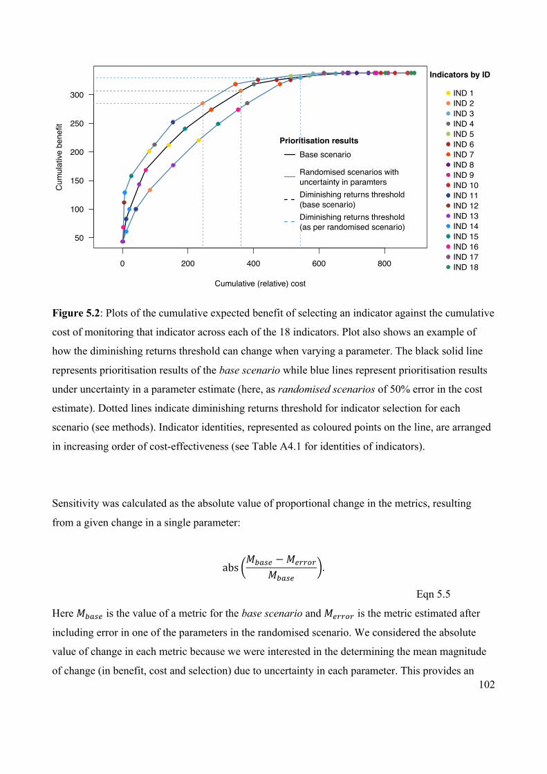
102

Figure 5.2: Plots of the cumulative expected benefit of selecting an indicator against the cumulative

cost of monitoring that indicator across each of the 18 indicators. Plot also shows an example of

how the diminishing returns threshold can change when varying a parameter. The black solid line

represents prioritisation results of the base scenario while blue lines represent prioritisation results

under uncertainty in a parameter estimate (here, as randomised scenarios of 50% error in the cost

estimate). Dotted lines indicate diminishing returns threshold for indicator selection for each

scenario (see methods). Indicator identities, represented as coloured points on the line, are arranged

in increasing order of cost-effectiveness (see Table A4.1 for identities of indicators).

Sensitivity was calculated as the absolute value of proportional change in the metrics, resulting

from a given change in a single parameter:

absÑÖÜ:á − ÑáVVàV

ÑÖÜ:á.

Eqn 5.5

Here ÑÖÜ:á is the value of a metric for the base scenario and ÑáVVàV is the metric estimated after

including error in one of the parameters in the randomised scenario. We considered the absolute

value of change in each metric because we were interested in the determining the mean magnitude

of change (in benefit, cost and selection) due to uncertainty in each parameter. This provides an

0 200 400 600 800

50

100

150

200

250

300

Cumulative (relative) cost

Cum

ulat

ive b

enef

it

Base scenario

Randomised scenarios withuncertainty in paramtersDiminishing returns threshold(base scenario)Diminishing returns threshold(as per randomised scenario)

Prioritisation results

IND 1IND 2IND 3IND 4IND 5IND 6IND 7IND 8IND 9IND 10IND 11IND 12IND 13IND 14IND 15IND 16IND 17IND 18

Indicators by ID

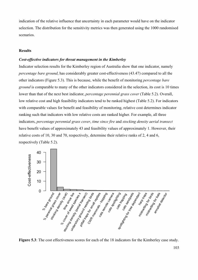
103

indication of the relative influence that uncertainty in each parameter would have on the indicator

selection. The distribution for the sensitivity metrics was then generated using the 1000 randomised

scenarios.

Results

Cost-effective indicators for threat management in the Kimberley

Indicator selection results for the Kimberley region of Australia show that one indicator, namely

percentage bare ground, has considerably greater cost-effectiveness (43.47) compared to all the

other indicators (Figure 5.3). This is because, while the benefit of monitoring percentage bare

ground is comparable to many of the other indicators considered in the selection, its cost is 10 times

lower than that of the next best indicator, percentage perennial grass cover (Table 5.2). Overall,

low relative cost and high feasibility indicators tend to be ranked highest (Table 5.2). For indicators

with comparable values for benefit and feasibility of monitoring, relative cost determines indicator

ranking such that indicators with low relative costs are ranked higher. For example, all three

indicators, percentage perennial grass cover, time since fire and stocking density aerial transect

have benefit values of approximately 43 and feasibility values of approximately 1. However, their

relative costs of 10, 30 and 70, respectively, determine their relative ranks of 2, 4 and 6,

respectively (Table 5.2).

Figure 5.3: The cost effectiveness scores for each of the 18 indicators for the Kimberley case study.

104

Table 5.2: Values for the cost (Ci), benefit (Bi), feasibility (Fi) and cost-efficiency (Ei) of indicators

for the Kimberley case study, arranged in decreasing order of their cost efficiency.

Rank ID Indicator Cost Benefit Feasibility Cost effectiveness

1 12 Percentage bare ground 1 43.47 1 43.47

2 11 Percentage perennial grass cover 10 39.21 0.9 3.92

3 14 Stocking (exotic herbivore) density - indirect (scat) 10 17.39 0.8 1.74

4 13 Time since fire 30 43.47 1 1.45

5 16 Percentage cover of weed species x 20 24.73 0.8 1.24

6 1 Stocking (exotic herbivore) density - aerial transect 70 43.47 1 0.62

7 15 Relative abundance of understory and ground nesting birds

50 28.91 0.8 0.58

8 7 Pitfall traps for small reptiles 80 33.26 0.8 0.42

9 2 Relative abundance of CWR mammals - trapping 90 33.26 0.8 0.37

10 4 Cats remote camera 40 11.33 1 0.28

11 6 Cats spotlighting 70 7.37 0.6 0.11

12 5 Cats trapping 100 7.1 0.4 0.07

13 3 Cats sand pads 80 3.97 0.5 0.05

14 17 Spotlighting for tree dependant animals 40 1.13 0.5 0.03

15 8 Harp traps 60 0 0.3 0

15 9 Mist netting for birds 60 0 0.5 0

15 10 Mist netting for bats 60 0 0.3 0

15 18 Anabat detector 20 0 0.3 0

Monitoring indicators additional to the most cost-effective indicator, percentage bare ground

(indicator 12), incurs little additional cost but increases the expected benefit three-fold (Figure 5.4).

These include percentage perennial grass cover, stocking density-indirect, time since fire and

percentage cover of weed species. Nine indicators were selected in total for the Kimberley case

study when using the diminishing returns threshold. Together these provide a cumulative expected

benefit of 345.9 (which represents the sum of the improvement in species persistence across all

105

species groups and management for all threats), for a total relative cost of monitoring of 361.

Monitoring additional indicators beyond the point of diminishing returns provides little additional

benefit. Selection based on cost-effectiveness of indicators provides a much higher cumulative

benefit relative to the cost as opposed to selection of indicators based only on the cost of monitoring

or the average probability of detecting change across all three threats for an indicator (Figure 5.4).

Comparing the number of indicators included in the top 9 under each scenario shows a change in

three of the indicators from the cost-effectiveness approach. Indicators 1, 7 and 2 selected using the

cost-effectiveness approach are replaced with indicators 18, 4 and 17 when the prioritisation is

based only on the cost of monitoring indicators; and the same three are replaced by indicators 9, 8,

6 and 5 when using the average probability of detecting change (see Table 5.2 for indicator

identifies).

Figure 5.4: Relationship between cumulative expected benefit of selecting an indicator and

cumulative cost of monitoring indicators in the Kimberley based on the cost-effectiveness approach,

Ei (black line) versus selection based only on cost of monitoring an indicator, Ci (blue line) or the

average probability of detecting change across threats for an indicator, )*+;+<1 (red line). Costs are

relative and have been rescaled to range between 1 and 100 (least and most expensive,

respectively). Values for probability of detecting change in each threat for each indicator (which are

0 200 400 600 800

010

020

030

040

0

Cumulative (relative) cost

Cum

ulat

ive b

enef

it

dim

inis

hing

retu

rns

th

resh

old

12

1114

1316

115

72 4 6 5 3 17

8 9 10 18

12

111416 18

13 417

15 8 9 10

1 6

7 32 5

9

1115 8 6

16

1213

5 3

114 17 10

72 4 18

Cost−effectiveness

Cost of monitoringAverage probability of detectingchange across threats

Prioritisation based on

106

averaged for the purpose of this figure) are provide in Table A4.3 in appendix 4.2. Indicator

identities are numbered on the lines in increasing order of cost-effectiveness (see Table A4.1 for

identities of indicators).

Sensitivity analysis

Results of the sensitivity analysis are shown as the magnitude of the proportional change in the four

sensitivity metrics: (1) metric 1: Spearman rank correlation between rankings of selected indicators

for the base and randomised scenario; (2) metric 2: the expected benefit of monitoring selected

indicators up to the point of diminishing returns (i.e. sum of the benefits); (3) metric 3: the total cost

of monitoring selected indicators up to the point of diminishing returns (i.e. sum of the costs); and

(4) metric 4: change in the identities of indicators selected up to the point of diminishing returns

(i.e. number of indicators that are different between the base and randomised scenario selection).

These metrics show the extent to which varying each parameter, and thus the uncertainty in

parameter estimates, changes the indicator selection as compared to the base scenario. We explored

the sensitivity of the indicator selection approach to uncertainty in parameter estimates over a range

of error levels (from 0 to 50 %) in parameter estimates (Figure 5.5). Note that for metric 1, smaller

values indicate higher sensitivity, unlike for metric 2, metric 3, and metric 4.

Sensitivity of the parameters depends on the metric being used. Indicator selection was more

sensitive to the parameter t+ (i.e. prior belief in the impact of a threat) when using metric 2 (µ = ~

0.2) as compared to metric 4 or metric 4 (µ = 0). The order of sensitivity of parameters also varied

according to the metric used. Indicator selection was most sensitive to error in )*+ (i.e. probability

of detecting a change in threat with an indicator) in case of metric 1, metric 3 and metric 4 and least

sensitive to error in u* (i.e. feasibility of monitoring an indicator) in case of metric 2, metric 3 and

metric 4. This implies that indicator selection is influenced to varying degrees by uncertainty in the

different parameters. In some cases, there was significant overlap in sensitivity of indicator

selection to error in the parameters, e.g. error in t+, u+, and 5+ had similar influence whereas error u*

clearly had a significantly smaller influence on indicator selection (Figure 5.5b). Interestingly, up to

20% error in some parameter estimates resulted in no change in the sensitivity metrics, e.g. for t+

(i.e. prior belief in threat impacts) in metric 1, metric 3 and metric 4. This implies that indicator

selection remains unchanged despite low levels of uncertainty in t+. This is also the case for u* (i.e.

feasibility of monitoring an indicator) when using metric 2, metric 3 and metric 4.

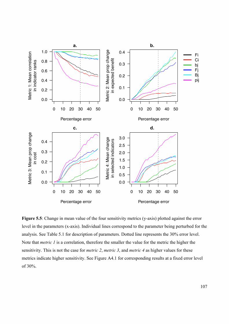
107

Figure 5.5: Change in mean value of the four sensitivity metrics (y-axis) plotted against the error

level in the parameters (x-axis). Individual lines correspond to the parameter being perturbed for the

analysis. See Table 5.1 for description of parameters. Dotted line represents the 30% error level.

Note that metric 1 is a correlation, therefore the smaller the value for the metric the higher the

sensitivity. This is not the case for metric 2, metric 3, and metric 4 as higher values for these

metrics indicate higher sensitivity. See Figure A4.1 for corresponding results at a fixed error level

of 30%.

0 10 20 30 40 50

0.0

0.2

0.4

0.6

0.8

1.0

Percentage error

Met

ric 1

: Mea

n co

rrela

tion

in in

dica

tor r

anks

0 10 20 30 40 50

0.0

0.1

0.2

0.3

0.4

Percentage error

Met

ric 2

: Mea

n pr

op c

hang

ein

exp

ecte

d be

nefit

0 10 20 30 40 50

0.0

0.1

0.2

0.3

0.4

Percentage error

Met

ric 3

: Mea

n pr

op c

hang

ein

cos

t

0 10 20 30 40 50

0.00.51.01.52.02.53.0

Percentage error

Met

ric 4

: Mea

n ch

ange

in s

elec

ted

indi

cato

rs

FiCibjFjBjpij

a. b.

c. d.

108

Discussion

Choosing indicators for informing management decisions is complicated because different

indicators vary in their costs of monitoring as well as in the information they provide, naturally

leading to the question of which indicator should be monitored. Methods used to select indicators

need to identify those indicators that deliver the greatest benefit per unit cost (Nichols & Williams

2006; Mace & Baillie 2007). Although studies have evaluated the cost-effectiveness of alternate

indicator choices (Tulloch, Possingham & Wilson 2011; Peck et al. 2014), approaches to do so

when indicators need to inform on multiple threats and their management are lacking. In this study,

we propose that an informed indicator choice when multiple threats are present requires knowing

about factors related to the monitoring efficiency, management outcomes and the economic

constraints for decision-making to estimate the cost-effectiveness of indicators. We provide a

systematic and logical approach to integrate these factors in a single decision framework to

determine the most cost effective indicators. Through the use of a case study, we show that when

managers need to consider monitoring and managing multiple threats on biodiversity, considering

individual factors like cost or probability of detecting a change to select indicators is not sufficient

(Figure 5.4). Instead, a cost-effectiveness approach that accounts for the management context as

well as the economic constraints for decision-making is likely to deliver better outcomes.

Indicators are often selected based simply on whether they are sensitive to change or if they are

cheap to monitor (Heink & Kowarik 2010b; Siddig et al. 2016), rather than on a combination of

these and other factors. Clearly, these are important considerations to ensure that indicators do not

fail to detect significant environmental change or lead to wasteful spending of resources on

monitoring. However, we show that additional criteria are required to explicitly evaluate each

threat-indicator-management intervention combination and ensure that the selected indicators can

trigger appropriate management interventions in the face of multiple threats. Our CE analysis

framework for indicator selection assumes that, all else being equal, an indicator is better if (1) it is

a proxy for multiple threats; (2) it informs us about a threat that is more significant compared to an

indicator of a threat that does not warrant management; (3) it is cheap and easy to monitor; (4) it is

reliable i.e. can detect a change in the level of threat rapidly and effectively; (5) it can trigger

appropriate management interventions i.e. helps monitor threats that have feasible and beneficial

management interventions available. Although similar factors or criteria have previously been

suggested (e.g. Heink & Kowarik 2010b; Lindenmayer et al. 2015), ours is the first approach to

109

integrate these factors in a quantitative economic assessment of competing indicator choices. This is

especially useful from decision-makers’ perspective as it can help prioritise spending on monitoring

indicators that provide the best outcomes from management in a transparent way. Most importantly,

we provide a framework that allows decision makers to be explicit about the costs and the multiple

factors influencing the benefits of monitoring alternative indicators.

It is interesting to note that three out of four highest ranked indicators (Table 5.2) are able to detect

only a single threat, fire and grazing. For the first three indicators selected, the high cost-

effectiveness can perhaps be explained by (a) the high feasibility to cost of monitoring ratio, and (b)

the high probability of detecting change in at least one out of the three threats (i.e. pij = 1).

However, the indicator – time since fire has high probability of detecting change in only one out of

the three threats but it had low feasibility to cost ratio. This indicates that the probability of change

detection and the cost to feasibility ratio are decisive parameters in indicator selection and are

possibly traded-off when evaluating the benefit and hence the cost-effectiveness of indicators. This

also highlights the importance of the selection of complementarity sets of indicators (as discussed

below) that can inform on the maximum number of threats and benefit the greatest number of

species per dollar spent. Low cost-effectiveness for an indicator can either arise if the indicator does

not inform on the threats (thereby leading to low benefit of monitoring) or if the benefit of

monitoring an indicator is traded-off against the other parameters, e.g. high cost or low feasibility of

monitoring the indicator. Our framework highlights that in some situations, a given indicator may

not provide any benefit for monitoring a particular threat (represented by the ‘zero-benefit’ nodes in

Figure 5.1). For example in the Kimberley, monitoring of cats using remote cameras cannot detect

changes in threats such as fire and grazing and weeds, thereby reducing the overall benefit of

monitoring cats (using remote cameras) as an indicator for managing multiple threats (see Figure

5.3 and Figure A4.2 in Appendix 4.3). However, even if an indicator informs on all three threats,

such as relative abundance of understory and ground nesting birds (see Table A4.3 in Appendix

4.2), it does not have the high cost-effectiveness possibly due to the higher costs of monitoring

(Table 5.2). Therefore, the overall cost-effectiveness of an indicator is a result of the trade-offs

between the factors considered for indicator selection. Such transparency in the indicator selection

process, as can be provided by our framework, allows decision-makers to make well-informed and

defensible judgments regarding their indicator choices.

110

The simplicity of the underlying analysis makes our approach easily adaptable to real-world

conservation decisions that may involve a large number of threats, species, management

interventions and potential indicators. This makes the cost-effectiveness approach for indicator

selection preferable over methods that may be computationally challenging and therefore less likely

to be taken up by conservation practitioners (Auerbach, Tulloch & Possingham 2014). Examples of

such challenging approaches include value of information, an approach to identify the best way to

expend efforts on collecting data to improve a decision through reducing uncertainty (Howard

1966), or optimisation methods that seek to achieve multiple objectives under certain constraints

(e.g. maximizing feasibility and/or benefits whilst minimizing costs; Tulloch et al 2013). Moreover,

the information required for such the CE analysis can be obtained from experts with knowledge of

the relevant ecosystems using any one of a variety of well-established elicitation techniques to

ensure that expert judgments are as reliable and unbiased as possible (e.g. Kuhnert, Martin &

Griffiths 2010; Martin et al. 2012a; McBride & Burgman 2012).

The credibility and utility of a decision-making model or method depends on knowing the

importance of each parameter for the results of the model or method (Norton 2015). Sensitivity

analysis is a useful way to identify the relative contributions of the different sources of uncertainty

in model inputs to the model output (Saltelli et al. 2008). In our framework, if the parameters

influence the cost-effectiveness of indicators and their rankings to varying degrees, then uncertainty

in some parameters is more likely to influence decisions than uncertainty in other parameters. From

a decision-making context, certain sensitivity metrics are more useful than others. For instance, in

our view, change in the identities of selected indicators (metric 4) is of highest utility as it indicates

variability in decisions, i.e. selected indicators, due to uncertainty. On the other hand, the Spearman

rank correlation between indicator rankings from two selections (metric 1) is of least utility because

the metric weights change in the lowest ranked indicators as equally important as change in the

highest ranked indicators. This is not sensible because we rarely care about the lowest ranked

indicators with the lowest cost-effectiveness scores, as these will never be selected for monitoring.

When sensitivity metrics are used in conjunction with one another, they can provide complementary

information for effective indicator selection. For instance, a decision maker may be interested in

knowing the effect of uncertainty on the benefit of monitoring and how it might adversely affect her

choice of indicators (i.e. metric 2 and metric 4, respectively). Here, she may compare parameter

sensitivities using both the metrics to identify the ones that when improved upon can give the

largest decrease in uncertainty across multiple measures, e.g. )*+ and u+ (Figures 5.5b and 5.5d).

111

Finally, although our cost-effectiveness framework accounts for Type II error by specifying a

probability of detection ()*+) and testing the sensitivity of this parameter for monitoring choices, the

potential for both Type I and Type II errors in identification of optimal indicators needs further

evaluation.

The cost-effectiveness (CE) approach assumes that all parameters are independent. However in

some cases there may be dependencies between indicators (e.g. indicators with shared costs), which

can be incorporated to improve indicator selection using the cost-effectiveness approach (Auerbach

et al. 2015). For instance, indicators for monitoring vegetation (percentage bare ground,

percentage perennial grass cover and percentage cover of weed species), or those that require

setting up of mist-nets (mist-netting for birds and mist-netting for bats) may be monitored together

to reduce overall monitoring costs. Alternately, in case indicators have shared costs, such that

monitoring one indicator changes monitoring costs of the other indicators considered in the

selection, we could use a greedy algorithm as is currently implemented, except where cost

parameter values and therefore cost-effectiveness estimates are recalculated after each new

indicator is selected (Possingham, Ball & Andelman 2000). In the Kimberley case study,

percentage bare ground is likely to be selected in spite of correlation in the parameters because it is

significantly more cost-effective than any of the other indicators considered in the selection.

However, correlation might change the rankings of some of the other indicators. On the other hand,

some indicators may provide information on the same threats, e.g. three out of the four highest

ranking indicators for the Kimberley i.e. percentage bare ground, stocking density – indirect and

time since fire can detect changes in only one threat (fire and grazing) while failing to account for

the other threats present in the system (Table A4.3). In order to improve cost-effectiveness of

selected indicators, we can opt for a complementary set of indicators that maximize the number of

threats represented in the selection (Tulloch, Chadès & Possingham 2013). To do so, we choose

down the ranked list but we do not select indicators for a particular threat once the threat has

already been represented in the selection.

While the results of the case study presented here were based on values elicited from one expert, in

reality the knowledge of multiple experts would likely provide more accurate estimates (Kuhnert,

Martin & Griffiths 2010; McBride & Burgman 2012). However, the purpose of this study is to

demonstrate the cost-effectiveness framework for indicator selection. For using our methods to

inform real-life conservation decisions, we suggest using robust elicitation approaches using

112

multiple experts such as the Delphi process (MacMillan & Marshall 2006). This involves a diverse

set of people with differing levels of expertise (Burgman et al. 2011) and an iterative process of

feedback and revision to elicit individual estimates (Kuhnert, Martin & Griffiths 2010; Martin et al.

2012a). Additionally, experts can be asked to provide their best estimates of parameters, lower and

upper bounds on these estimates and a level of confidence that the true estimate lies within the

nominated lower and upper bounds (Kuhnert, Martin & Griffiths 2010; Martin et al. 2012a).

Adopting structured and robust procedures to gather expert judgments such as those mentioned

above have been shown to provide reliable estimates of known values and hence provide useful

information to inform decisions were data is limited (Burgman 2005).

As was the case with the previous chapters, here too the trade-offs between monitoring and

management allocation when decisions are being made under constrained resources have been

ignored, and we consider a one-time step decision-making process. Both these simplifying

assumptions, as in the case of chapters three and four, help establish a basic yet novel indicator

selection framework based on cost-effectiveness. However, this framework is only intended as a

first-step in the development of robust and adaptive selection approaches. Accounting for the costs

of monitoring would require evaluating not just the benefit of management actions, as is presently

done in our framework, but their cost-effectiveness. Therefore, we would have to consider not one

but two simultaneous prioritisation frameworks, one each for monitoring and management decision-

making. To do so, the costs of monitoring and management actions can be linked through some

functional relationship (e.g. correlation) and the two prioritisations can then be run in tandem. In

order to add a temporal component to the analysis, the elicited parameters can be made time-

specific, for example by discounting the cost of monitoring indicators as monitoring programs gets

established over time, or changing prior belief in impacts of threats based on information in the

previous time step or based on seasonal changes threat in a landscape. Parameter estimates for each

time-step required for the analysis can be obtained in a number of different ways, for example by

conducting meta-analyses of existing studies, through expert elicitation (e.g. Runge, Converse &

Lyons 2011), modeling or through empirical studies (e.g. Johnson et al. 2014). The cost-

effectiveness analysis and indicator prioritisation could then be conducted iteratively, for instance

every 5 years, to provide best indicator choices over time.

Our cost-effectiveness analysis framework for selecting indicators for managing multiple threats

provides a systematic method for explicitly linking indicator choices to management decisions. An

113

expert-based approach such as ours, offers substantial scope for collaboration between researchers

and managers when thinking about indicators for management decision-making. Owing to the

simplicity of the cost effectiveness formulation, it has the added advantage of being easily adaptable

to complex real-world decisions as well as being easily accessible to conservation practitioners and

decision-makers. By ensuring that indicators are selected to maximise impact given limited

resources in a systematic, logical and transparent way, our approach provides a marked

improvement over ad-hoc selection methods.

Acknowledgements


Environmental Decisions, the School Research Grant from the School of Geography, Planning and

Environmental Management at the University of Queensland and a University of Queensland

International Scholarship. We thank Sarah Legge of the Australian Wildlife Conservancy for

providing expert advice on the details of the Kimberley case study and Ascelin Gordon for feedback

on the analysis.

114

Chapter six

Discussion

115

Chapter six - Discussion

Synthesis

The importance of monitoring biodiversity in ecology and conservation science is undisputed, be it

for understanding ecosystem state or deciding how to intervene to conserve biodiversity (Nichols &

Williams 2006; Possingham et al. 2012). This latter role of monitoring to support management

decisions is being increasingly realised (Yoccoz, Nichols & Boulinier 2001; Nichols & Williams

2006) due to the growing threats to biodiversity and the limited resources available to mitigate these

threats. As a result, there has been a steady increase in the application of concepts from economics

and decision science to develop optimal monitoring approaches for conservation decision-making

(e.g. Maxwell & Jennings 2005; Conroy, Stodola & Cooper 2012; Tulloch, Chadès & Possingham

2013; Wilson, Rhodes & Possingham 2015). However, monitoring to inform management when

biodiversity is faced with multiple threats has received relatively little attention. To address this

gap, this thesis had four main objectives: (1) to review current approaches for selecting indicator

species for biodiversity management; (2) to assess the value of monitoring species for managing

multiple threats; (3) to assess the relative influence of uncertainty and expected benefits of

management on monitoring decisions for multiple threats; and (4) to develop a simple indicator

selection tool based on a return on investment framework for managing multi-species, multi-threat

systems. In addressing these objectives, this thesis develops insights for systems where there is a

range of possible monitoring options, and develops new tools for evaluating and selecting

monitoring strategies for management decision-making.

In this concluding chapter, I briefly summarise the core contributions of each chapter of the thesis

and discuss their implications for biodiversity conservation. I then discuss potential limitations and

suggest avenues for future research.

Selecting indicator species for biodiversity management

Indicator species are commonly used to inform biodiversity management. In chapter two, I

reviewed the scientific literature to assess if indicator species intended for management decision-

making are selected using clear management objectives and evaluated for their ability to improve

management outcomes. I show that indicator research continues to be rooted in the traditional

approach of selecting indicators to adequately represent natural systems, therefore improving the

116

monitoring efficiency rather than the management effectiveness. Moreover, indicator selection

rarely considers decision factors, such as objectives, constraints (e.g. budget), actions (e.g.

alternative indicators), uncertainties (e.g. in detection or management effectiveness) and outcomes

for management. The literature shows that ignoring management decision factors such as

objectives, constraints and uncertainty can have profound consequences as selected indicators may

mislead management decision-making (Lindenmayer, Piggott & Wintle 2013), may not be cost-

effective (Tulloch, Chadès & Possingham 2013) or they may overestimate the benefit of monitoring

to improve decisions (Lyons et al. 2008). The results from this chapter highlight the need to move

beyond the much-cited trade-off between measurement accuracy and practical constraints of

monitoring indicators (Lindenmayer et al. 2015), to a full clarification of the management decision

factors that govern indicator choice. To address this need, I suggest the use of a structured decision-

making framework for selecting indicators along with (a) clearly defining the management context

for monitoring, (b) developing practical methods focused on improving management outcomes, and

(c) incorporating uncertainty into the selection process to improve indicator selection for

management decision-making.

The value of monitoring species to manage multiple threats

Most species are impacted by multiple threats that in concert play a role in observed species

declines (Brook, Sodhi & Bradshaw 2008). When the conservation objective is to conserve multiple

species facing multiple threats, monitoring decisions need to account for their impacts, which may

be cumulative, as well as the link between each threat and the response of different species to these

threats. In chapter three, I developed and tested the value of information (VOI) approach for

investigating how monitoring alternative species, as in the case of indicator species, subject to

multiple threats improves our ability to inform the management of these threats. Overall, this

chapter contributes two main advances for optimal monitoring approaches for biodiversity

conservation. Firstly, this is the first study to utilise the VOI approach to identify monitoring

strategies that inform decisions about threat management when multiple threats are operating and

multiple species are at stake. Secondly, it provides insight into when species monitoring is likely to

be of value to threat management. The results show that without an experimental design to learn

about how species respond to threats in the system, monitoring species alone may be ineffective in

directing threat management actions among multiple threats. In other words, a non-experimental

monitoring design provides little or no information for management decision-making and therefore

does not improve conservation outcomes from management compared to experimental monitoring

117

(monitoring with experimentation to explicitly learn about threats). These results have major

implications for biodiversity conservation because taking a non-experimental monitoring approach,

the most common form of conservation monitoring (Nichols & Williams 2006), may contribute to a

failure to arrest species declines, and at worst, lead to extinctions.

Uncertainty in monitoring decision-making

Monitoring to inform the management of multiple threats is complex because species responses to

threats and their management are variable and often highly uncertain. Although monitoring is often

framed from the point of view of reducing uncertainty, a reduction in uncertainty is only valuable

from a management point of view if it improves management decisions (Maxwell et al. 2015). In

chapter four, I demonstrated the use of VOI analysis to establish the value of monitoring to inform

management given uncertainty in the effectiveness of alternative management actions and identify

the optimal monitoring strategy. This chapter provides a stochastic exponential growth population

model to develop a novel formulation of the VOI approach. It uses the change in population growth

rate to assess the effect of management of a threat on the species, and represents uncertainty as the

variance in the growth rate estimate. By mathematically formulating the relationships between VOI,

expected benefit of management and the uncertainty in management effectiveness, this chapter

provides two key insights for decision-making under uncertainty for multi-threat systems. First,

monitoring is found to be beneficial when management actions are thought to have similar effects

on the threats and this benefit increases with increasing uncertainty. Second, in these cases,

monitoring the action with the greater uncertainty always provides a higher benefit. Importantly,

this chapter demonstrates that monitoring need not always target threats and management actions

with the highest perceived impacts on biodiversity. Unlike the formulation presented in chapter

three, this formulation can more easily be extended to systems with more species owing to the use

of a stochastic population growth model.

Cost-effective monitoring to trigger conservation interventions

Choosing indicators for informing management decisions is complicated because different

indicators vary in their costs of monitoring as well as in the information they provide, naturally

leading to the question of which indicator should be monitored. Managers need a practical and

approachable method for selecting cost-effective indicators for managing under constrained budgets

and with the decision context in mind. In chapter five, I developed and tested a return on

investment framework based on estimating the cost-effectiveness of monitoring indicators for

118

triggering threat management actions in multi-species, multi-threat systems. I developed six factors

spanning monitoring efficiency, management outcomes and the economic constraints for decision-

making to estimate the cost-effectiveness of indicators. Because this framework accounts for

multiple criteria, it improves on common approaches whereby indicators may often be selected

based only on whether they are sensitive to change or cheap to monitor (e.g. de la Nuez-Hernandez

et al. 2014; Brunbjerg et al. 2015). The results show that indicator selection based on a cost-

effectiveness framework can help improve threat management decisions when resources are

limited, leading to better conservation outcomes. My work extends previous literature on indicator

cost-effectiveness (e.g. Tulloch et al. 2011, Tulloch et al. 2013) as the analysis framework

explicitly accounts for the management implications of monitoring, when selecting indicators for

managing multiple threats. This chapter contrasted the more formal, quantitative approaches of the

previous chapters with a desire to provide a relatively simple approach to help prioritise spending

on monitoring strategies that provide the best conservation outcomes under limited resources.

Overarching Contributions

Taking lessons from decision theory, structured decision-making and the optimal monitoring

literature, my thesis focuses on two key areas of research: theory development (chapters two, three

and four) and tool development (chapter five) to support managers in choosing monitoring

strategies for effective biodiversity management under uncertainty. The overall contributions of this

thesis to the theory and practice of optimal monitoring for conservation decision-making are as

follows:

1. This thesis exposes the gap in the conservation literature between indicator selection approaches

and the management decision context governing indicator choice (chapter two).

2. It suggests ways to frame monitoring choices in a structured decision-making process by

explicitly considering the management objective for monitoring and evaluating monitoring

choices in light of the objectives, constraints and uncertainties for management.

3. It sets out an overarching framework to make monitoring choices, based on structured decision-

making, and identifies a number of quantitative methods to critically evaluate monitoring

choices for management decision-making (chapter two).

4. It illustrates the use of the framework to evaluate monitoring choices by applying it to case

studies representing typical conservation scenarios, specifically for multi-species, multi-threat

119

systems (chapters three, four and five). These three chapters also demonstrate the utility of

some of the decision-analytic approaches identified in chapter two to evaluate monitoring

choices based on their costs and benefits for management.

5. It develops the underlying theory for selecting optimal monitoring and management strategies

for multiple threats. Here, I focussed on assessing the benefit of different types of monitoring

approaches (species monitoring, experimental versus non-experimental monitoring; chapter

three) and the role of uncertainty for decision-making (chapter four).

6. This thesis also develops a simple tool for real-world conservation decision-making based on a

return-on-investment framework (chapter five). The tool allows managers to prioritise the cost-

effectiveness of alternative monitoring choices when managing for multiple threats.

In any kind of decision-making scenario for conservation, managers use a number of different types

of strategies for monitoring biodiversity and how it responds to environmental change and

management interventions. The decision frameworks for monitoring proposed in my thesis, are

widely applicable across different types of monitoring strategies and indicators, from species-

specific scientific monitoring programs to those that incorporate remote sensing data or community-

based biodiversity monitoring. Above all, this thesis emphasises the need to adhere to consistent

methodologies to identify, measure and monitor biodiversity to make sure that the approaches used

for monitoring can most effectively support the conservation of biodiversity.

At the same time, the thesis draws attention to the way in which scientists and practitioners define

metrics for monitoring biodiversity and management effectives. One could argue that there are thee

classifications of measures of biodiversity: (a) direct measures, as discussed previously, that target

the management objective specifically (e.g., using your example, attempting to sample the complete

biodiversity of the system of interest); (b) indicators which represent a subset of the specific

management objectives (e.g., presence/absence of particularly sensitive or representative members

of the stream community); and (c) proxy measures which are attributes of the system that might be

more easily measured than fundamental management targets themselves but are believe to be

strongly correlated with the stated objectives. Although indicators and proxies can be considered

philosophically equivalent (neither are true, direct measures of the management objective), they are

often operationally distinct in that indicators are partial, direct measures of objectives while proxies

are indirect but related under the assumption of correlation.

120

Limitations and future research

The research presented in this thesis addresses some of the many challenges in identifying optimal

monitoring strategies for biodiversity conservation. In this section, I outline further research

priorities and discuss existing studies and approaches that may be useful to address these priorities.

Science versus practice

The review of the scientific literature selecting indicator species for management (chapter two)

revealed a number of approaches and factors that should be considered when selecting and

evaluating indicator species. However, decisions are often made based on decision-makers’ beliefs

and values, past experiences, associations, habits or obvious preferences rather than solely on

scientific evidence (Kahneman 2013; von Winterfeldt 2013). Even when decision-makers rely on

scientific evidence, they may not be aware of, or have the ability to apply the most complex and up-

to-date decision-theoretic methods, nor may they have the same concerns as researchers regarding

multiple uncertainties and their impacts on management outcomes (Tulloch et al. 2016b). This

raises an interesting question: how do managers and decision-makers select indicator species to

inform management actions or evaluate management effectiveness compared to the approaches

proposed in the scientific literature? Conducting a more comprehensive review of selection

approaches by surveying management plans and/or interviewing decision makers could provide

valuable insight on the criteria that are currently steering real world monitoring choices. This

contextual information could allow further refinements of the tools and methods proposed in this

thesis.

Interactions

The decision-making frameworks developed in this thesis to select optimal monitoring strategies in

multi-species, multi-threat systems (chapters three, four and five) do not consider interactions

among species, or among threats. However, species form complex network structures through

interactions such as competition, predation, mutualism; and threats may interact to have non-

additive impacts on biodiversity (Brook, Sodhi & Bradshaw 2008; Auerbach et al. 2015). If the

correlations between threats or species are understood, then in some cases monitoring a single

species could provide information on the influence of multiple threats and/or the response of

multiple species. Furthermore, the proposed frameworks in this thesis considered management

actions and their effects on multiple threats to be independent. This is again a necessary

121

simplification for developing the theoretical background for the VOI approach as applied to

managing complex systems. Although it may not always be a reasonable approximation, e.g. in

ecosystems where the biota is impacted by increased fire frequency and invasive predators,

managing fire may reduce the impact of predators because of increased vegetation cover and shelter

for ground dwelling terrestrial animals (Russell, Smith & Augee 2003). Studies in optimal

monitoring have only dealt with a few of these interactions at a time. For instance, Tulloch, Chadès

and Possingham (2013) establish a surrogacy metric to assess how representative species are of one

another based on similarities in their behavioural ecology, threat level and habitat use overlap when

selecting indicators for management decision-making. Recent studies in conservation management

suggest ways to include species interactions networks (e.g. Tylianakis et al. 2010, Madden et al.

2016, Baket et al. 2016), impacts of multiple interacting threats (e.g. Mantyka-Pringle et al. 2015),

and dependencies in management actions (Evans, Possingham & Wilson 2011; Auerbach et al.

2015) in decision-making. These studies demonstrate the use of optimisation, Bayesian belief

networks, cost-effectiveness analysis and return on investment frameworks in decision-making

when incorporating interactions. Although the complexity of accounting for interactions to select or

evaluate monitoring choices is daunting, it has the potential to significantly improve monitoring

choices for multi-species, multi-threat management.

Monitoring accuracy

Optimal management decisions depend on the ability to correctly detect system states or trends

(Field et al. 2005; Wilson, Rhodes & Possingham 2015). Two kinds of errors influence monitoring

decisions: mistakenly concluding there is an effect when there is none (Type I error) and failing to

detect an effect where there is (Type II error) (Di Stefano 2003; Field et al. 2004). The proposed

VOI approach for evaluating monitoring choices in multi-species, multi-threat systems (chapters

three and four) assumes perfect detection thereby eliminating Type I and Type II errors from the

decision problem. As noted in these chapters, this is an approximation as we can rarely monitor the

state of an ecological system with high accuracy (Regan, Chadès & Possingham 2011). In multi-

species, multi-threat systems, a Type I error could result in misguided management interventions

that do not target the most important threats in the system leading to inefficient use of the limited

resources available for management. However, Type II errors are generally more important for

decision-making. They can result in the required management interventions not being implemented

in time or discontinued prematurely (Mapstone 1995; Field et al. 2004), potentially leading to

species declines due to the absence of effective or timely management (Martin et al. 2012b;

122

Lindenmayer, Piggott & Wintle 2013). In fact, given that biodiversity continues to decline globally

and that resources for management are limited, any erroneous conclusion (due to either a Type I or

a Type II error) would be cause for concern (Mapstone 1995).

Establishing the statistical power of monitoring, i.e. its ability to detect real outcomes

(1 – probability of a Type II error), is fundamental to ensure that monitoring is meaningful for

management decision-making (Field et al. 2007). Specifying an appropriate level of statistical

power however is not simply a statistical decision, but entails judgments about the biological

importance of an effect (Mapstone 1999) and the social, political and economic implications of the

resulting management or policy decisions (Possingham et al. 2001). Nevertheless, the potential for

errors in identifying optimal monitoring strategies for management must be explicitly

acknowledged and, where possible, evaluated for the alternative monitoring choices (see Mapstone

1995; Pollock et al. 2002; Tyre et al. 2003; Field et al. 2004; Field, Tyre & Possingham 2005;

Maxwell & Jennings 2005; Rhodes et al. 2006). Previous studies have used various methods to deal

with statistical errors in decision-making, for example decision-analysis to establish the risks of

overlooking Type 1 and Type II errors (Field et al. 2004), scenario and sensitivity analysis to

determine optimum statistical power for survey designs (Field, Tyre & Possingham 2005) and

Markov decision processes to allow dynamic updating of the observation probabilities over time

(Littman 2009; Regan, Chadès & Possingham 2011). The cost-effectiveness analysis developed in

this thesis for monitoring and managing multiple threats (chapter five) accounts for Type II error

by specifying a probability of detection and testing the sensitivity of this parameter for monitoring

choices. However, it does not deal with Type I errors. The optimal monitoring approaches proposed

in this thesis for multi-species, multi-threat management can be improved by adopting the

aforementioned methods to account for errors that may occur in the decision process, thereby

reducing the chance of making expensive mistakes for biodiversity management. Finally, the

expected value of sample information (chapter three) offers one possible way to incorporate

parameter uncertainty in the VOI analysis such as that resulting from imperfect detection (Yokota

& Thompson 2004).

Monitoring versus management

The focus of this thesis was the development of approaches for designing efficient and effective

monitoring strategies for complex systems under conditions of management (financial) constraints.

With such a practical, applied focus it is important to acknowledge that optimal decision-making for

123

conservation requires allocating resources between monitoring as well as management. In this

larger decision-context, making optimal monitoring decisions should not only involve evaluating

the benefits or cost-effectiveness of alternative monitoring choices for management (chapters

three, four and five), but also the risk involved in forgoing management gains when resources are

diverted for monitoring. This thesis did not consider optimising monitoring and management

decisions simultaneously, nor did it consider the different time horizons over which monitoring and

management actions may deliver benefits. The adaptive management literature explicitly addresses

these issues by balancing both short-term management gains and a desire to learn in order to

achieve optimal long-term management outcomes (Holling 1978; Walters & Holling 1990; Walters

& Green 1997; Hauser & Possingham 2008). Active adaptive management, in particular, provides a

protocol for examining the trade-off between learning and management when there is uncertainty

about how the system operates (Lyons et al. 2008; McDonald-Madden et al. 2010b). Other

approaches such as Partially Observable Markov Decision Processes have been applied to prioritise

management and survey effort (Chadès et al. 2008; Chadès et al. 2011). Extending the approaches

demonstrated in this thesis to include the trade-off between benefits and costs of alternate

monitoring and management actions would provide for a more holistic approach to tackle the more

general resource allocation problem for biodiversity conservation. Nevertheless, the optimisation of

monitoring, management, and learning in one framework comprises a mathematically complex

problem, which presents an exciting area for future research (McDonald-Madden 2008).

Timely decisions

Another consideration that was largely overlooked (at least explicitly) is the temporal dimension in

decision-making for monitoring. Chapters three and four consider one a time-step management

problem by maximising the objective function through one-off investment decisions for managing

threats. Although chapter five implicitly considered the temporal aspect in defining the parameter,

probability of persistence, which was estimated over 20 years for a given species, all other

parameters ignored the time horizons for decision-making. However, monitoring is rarely limited to

assessing system state at a single point in time, but is often used sequentially to either understand

parameters governing dynamical systems, track state conditions over time for guiding decision

thresholds (triggers), or learn over time from repeated decisions (adaptive management)

(Spellerberg 2005, Possingham et al. 2012). Moreover, systems and decision problems are

inherently dynamic, implying that monitoring choices may change within the course of a

management program. The inclusion of time-specific parameters for management actions,

124

monitoring actions or system dynamics can be added to the models used in this thesis. For example,

discounting the cost of monitoring indicators in chapter five as monitoring programs gets

established over time. By explicitly considering the time horizons over which the parameters used

in the models seem sensible for real-world management decisions, indicator selection and

prioritisation can be conducted iteratively, for instance every 5 years, to provide the best indicator

and management choices over time. Additionally, using the VOI approach within an adaptive

management framework could provide optimal monitoring (and management) solutions for

dynamic decision-making processes (Williams, Eaton & Breininger 2011). This requires specifying

a dynamic natural resource management problem over a discrete timeframe, in case of chapters

three and four, in response to changing environmental conditions and time-specific management

actions and actions that are taken sequentially over the time frame (Williams, Eaton & Breininger

2011). The returns (objective function) would depend on the system state and the action at every

time step, and are accumulated over time. Uncertainty can be tracked through time along with the

status of the managed resource by considering multiple transition models that reflect differing

beliefs regarding system dynamics (Williams, Eaton & Breininger 2011). As a result, different

points in the management time horizon will have different optimal decisions due to the different

priors.

Larger systems

The decision-making frameworks developed in this thesis, to select optimal monitoring strategies in

multi-species, multi-threat systems (chapters three and four) deal with a limited number of

species and threats. An obvious next step in order to improve their applicability to conservation is to

incorporate more complex systems with greater numbers of threats and/or species. This is especially

relevant given the shift in conservation focus from managing rare or endangered species to

ecosystem- and landscape-level conservation that attempts to manage multi-scale ecological

patterns and processes to sustain the full spectrum of biodiversity (Poiani et al. 2000; Tylianakis et

al. 2010; Gonthier et al. 2014). For instance, designing and managing reserve networks, climate

change mitigation and regional priority threat management, all require accounting for numerous

threats, threatened biota and larger sets of possible combinations of management actions (e.g.

Heller & Zavaleta 2009; Carwardine et al. 2012; Chadès et al. 2015; Firn et al. 2015). This thesis

has produced some of the underlying theory for such approaches, though much more remains to be

done. For instance, I have shown theoretically how a VOI formulation based on a population

growth model (chapter four) can easily be extended to include more species to establish the benefit

125

of monitoring for managing larger systems (Appendix 3.4), but the formulation needs further

development to account for greater number of threats. Alternatively, the cost-effectiveness

framework for indicator selection (chapter five) considers a larger set of species to protect as well

as indicators to choose from, and can be easily extended to account for greater number of threats.

However, unlike VOI, the cost-effectiveness framework has limited ability to evaluate the benefits

of reducing uncertainty in terms of improved decision-making regarding indicator choice.

Therefore, it cannot help identify the parameters for which more information would most improve

management decisions.

Concluding remarks

Ecological monitoring and the identification of indicators is a crucial component of conservation

science and practice. Providing better guidelines for monitoring to inform the management of

biodiversity is a necessary step towards better use of resources for conservation decision-making.

This thesis advances our understanding of both the challenges, and solutions required for

monitoring to make more effective decisions, particularly when multiple threats are operating and

multiple species are at stake. In doing so, my thesis addresses the repeated calls for monitoring to be

better suited to informing policy and actions for biodiversity conservation (Nichols & Williams

2006; Collen & Nicholson 2014).

126

Bibliography

Addison, P.F.E., de Bie, K. & Rumpff, L. (2015) Setting conservation management thresholds

using a novel participatory modeling approach. Conservation Biology, 29, 1411-1422.

Addison, P.F.E., Rumpff, L., Bau, S.S., Carey, J.M., Chee, Y.E., Jarrad, F.C., McBride, M.F. &

Burgman, M.A. (2013) Practical solutions for making models indispensable in conservation

decision-making. Diversity and Distributions, 19, 490-502.

Andelman, S.J. & Fagan, W.F. (2000) Umbrellas and flagships: Efficient conservation surrogates or

expensive mistakes? Proceedings of the National Academy of Sciences of the United States

of America, 97, 5954-5959.

ANZECC (2000) National water quality management strategy. No. 7a. Australian guidelines for

water quality monitoring and reporting. (ed. Australian and New Zealand Environment and

Conservation Council/Agriculture and Resource Management Council of Australia and New

Zealand). Canberra.

Auerbach, N.A., Tulloch, A.I.T. & Possingham, H.P. (2014) Informed actions: where to cost

effectively manage multiple threats to species to maximize return on investment. Ecological

Applications, 24, 1357-1373.

Auerbach, N.A., Wilson, K.A., Tulloch, A.I.T., Rhodes, J.R., Hanson, J.O. & Possingham, H.P.

(2015) Effects of threat management interactions on conservation priorities. Conservation

Biology, 29, 1626-1635.

Baker C.M., Gordon A., Bode M. (2016) Ensemble ecosystem modelling for predicting ecosystem

response of predator reintroduction. Conservation Biology. doi: 10.1016/j.tree.2016.04.009

Baker, J. & Gleed-Owen, C. (2007) National Amphibian and Reptile Recording Scheme. The

Herpetological Conservation Trust, Bournemouth, UK.

Bal, P., Tulloch, A.I.T., Addison, P.F.E., McDonald-Madden, E. & Rhodes, J.R. (in review)

Selecting indicator species for biodiversity management. Frontiers in Ecology and the

Environment.

Balmford, A., Gaston, K.J., Blyth, S., James, A. & Kapos, V. (2003) Global variation in terrestrial

conservation costs, conservation benefits, and unmet conservation needs. Proceedings of the

National Academy of Sciences, 100, 1046-1050.

127

Baxter, P.W., McCarthy, M.A., Possingham, H.P., Menkhorst, P.W. & McLean, N. (2006)

Accounting for management costs in sensitivity analyses of matrix population models.

Conserv Biol, 20, 893-905.

Beeton, R., Burbidge, A., Grigg, G., Harrison, P., How, R., Humphreys, W., McKenzie, N. &

Woinarski, J. (2010) Final report of the Christmas Island expert working group to the

Minister for Environment Protection, Heritage and the Arts.

Beliaeff, B. & Pelletier, D. (2011) A general framework for indicator design and use with

application to the assessment of coastal water quality and marine protected area

management. Ocean and Coastal Management, 54, 84–92.

Blanchard, J.L., Coll, M., Trenkel, V.M., Vergnon, R., Yemane, D., Jouffre, D., Link, J.S. & Shin,

Y.-J. (2010) Trend analysis of indicators: a comparison of recent changes in the status of

marine ecosystems around the world. ICES Journal of Marine Science, 67.

Bossel, H. (2001) Assessing viability and sustainability: a systems-based approach for deriving

comprehensive indicator sets. Conservation Ecology, pp. 12.

Breitburg, D.L., Baxter, J.W., Hatfield, C.A., Howarth, R.W., Jones, C.G., Lovett, G.M. & Wigand,

C. (1998) Understanding Effects of Multiple Stressors: Ideas and Challenges. Successes,

Limitations, and Frontiers in Ecosystem Science (eds M.L. Pace & P.M. Groffman), pp.

416-431. Springer New York, New York, NY.

Briggs, S.V. (2009) Priorities and paradigms: directions in threatened species recovery.

Conservation Letters, 2, 101-108.

Brook, B.W., Sodhi, N.S. & Bradshaw, C.J.A. (2008) Synergies among extinction drivers under

global change. Trends in Ecology & Evolution, 23, 453-460.

Brunbjerg, A.K., Jorgensen, G.P., Nielsen, K.M., Pedersen, M.L., Svenning, J.-C. & Ejrnaes, R.

(2015) Disturbance in dry coastal dunes in Denmark promotes diversity of plants and

arthropods. Biological Conservation, 182, 243-253.

Bunnefeld, N., Hoshino, E. & Milner-Gulland, E.J. (2011) Management strategy evaluation: a

powerful tool for conservation? Trends in Ecology & Evolution, 26, 441-447.

Burbidge, A.A., McKenzie, N.L., Brennan, K.E.C., Woinarski, J.C.Z., Dickman, C.R., Baynes, A.,

Gordon, G., Menkhorst, P.W. & Robinson, A.C. (2009) Conservation status and

biogeography of Australia’s terrestrial mammals. Australian Journal of Zoology, 56, 411-

422.

Burgman, M., Carr, A., Godden, L., Gregory, R., McBride, M., Flander, L. & Maguire, L. (2011)

Redefining expertise and improving ecological judgment. Conservation Letters, 4, 81-87.

128

Burgman, M., Lowell, K., Woodgate, P., Jones, S., Richards, G. & Addison, P. (2012) An endpoint

hierarchy and process control charts for ecological monitoring. Biodiversity Monitoring in

Australia (eds D.B. D. Lindenmayer & P. Gibbons), pp. 71-78. CSIRO Publishing,

Australia.

Burgman, M.A. (2005) Risks and decisions for conservation and environmental management.

Cambridge University Press, New York.

Butchart, S., Stattersfield, A., Baillie, J., Bennun, L., Stuart, S., Akçakaya, H., Hilton-Taylor, C. &

Mace, G. (2005) Using Red List Indices to measure progress towards the 2010 target and

beyond. Philosophical Transactions of the Royal Society B: Biological Sciences, 360, 255-

268.

Canessa, S., Guillera-Arroita, G., Lahoz-Monfort, J.J., Southwell, D.M., Armstrong, D.P., Chadès,

I., Lacy, R.C. & Converse, S.J. (2015) When do we need more data? A primer on

calculating the value of information for applied ecologists. Methods in Ecology and

Evolution, n/a-n/a.

Cardillo, M., Mace, G.M., Gittleman, J.L., Jones, K.E., Bielby, J. & Purvis, A. (2008) The

predictability of extinction: biological and external correlates of decline in mammals.

Proceedings of the Royal Society of London B: Biological Sciences, 275, 1441-1448.

Carignan, V. & Villard, M.-A. (2002) Selecting Indicator Species to Monitor Ecological Integrity:

A Review. Environmental Monitoring and Assessment, 78, 45-61.

Caro, T. (2010) Conservation by proxy: indicator, umbrella, keystone, flagship, and other surrogate

species. Island Press, Washington, DC

Carwardine, J., Klein, C.J., Wilson, K.A., Pressey, R.L. & Possingham, H.P. (2009) Hitting the

target and missing the point: target‐based conservation planning in context. Conservation

Letters, 2, 4-11.

Carwardine, J., Nicol, S., Van Leeuwen, S., Walters, B., Firn, J., Reeson, A., Martin, T.G. &

Chadès, I. (2014) Priority Threat Management for Pilbara Species of Conservation

Significance. pp. 72. CSIRO Ecosystem Sciences, Brisbane.

Carwardine, J., O'Conner, T., Legge, S., Mackey, B., Possingham, H. & Martin, T. (2011) Priority

threat management to protect Kimberley wildlife. pp. 76. CSIRO Ecosystem Sciences,

Brisbane.

Carwardine, J., O’Connor, T., Legge, S., Mackey, B., Possingham, H.P. & Martin, T.G. (2012)

Prioritizing threat management for biodiversity conservation. Conservation Letters, 5, 196-

204.

129

Chadès, I., Martin, T.G., Nicol, S., Burgman, M.A., Possingham, H.P. & Buckley, Y.M. (2011)

General rules for managing and surveying networks of pests, diseases, and endangered

species. Proceedings of the National Academy of Sciences, 108, 8323-8328.

Chadès, I., McDonald-Madden, E., McCarthy, M.A., Wintle, B., Linkie, M. & Possingham, H.P.

(2008) When to stop managing or surveying cryptic threatened species. Proceedings of the

National Academy of Sciences, 105, 13936-13940.

Chadès, I., Nicol, S., van Leeuwen, S., Walters, B., Firn, J., Reeson, A., Martin, T.G. &

Carwardine, J. (2015) Benefits of integrating complementarity into priority threat

management. Conservation Biology, 29, 525-536.

Christensen, P.E.S. (1980) The biology of Bettongia penicillata (Gray, 1837), and Macropus

eugenii (Desmarest, 1812) in relation to fire in Western Australia. pp. 1-90. Bulletin, Forests

Department, Western Australia.

Claxton, K., Ginnelly, L., Sculpher, M., Philips, Z. & Palmer, S. (2004) A pilot study on the use of

decision theory and value of information analysis as part of the NHS Health Technology

Assessment programme. Health Technol Assess, 8, 1-103, iii.

Cleary, D. (2006) The Questionable Effectiveness of Science Spending by International

Conservation Organizations in the Tropics. Conservation Biology, 20, 733-738.

Clemen, R. T. (1996) Making hard decisions: an introduction to decision analysis. Second edition.

Duxbury Press, Wadsworth, Belmont, California, USA.

Collen, B. & Nicholson, E. (2014) Taking the measure of change. Science, 346, 166-167.

Conroy, M.J., Stodola, K.W. & Cooper, R.J. (2012) Effective use of data from monitoring programs

and field studies for conservation decision making: predictions, designs and models working

together. Journal of Ornithology, 152, 325-338.

Cook, C.N., Carter, R.W., Fuller, R.A. & Hockings, M. (2012) Managers consider multiple lines of

evidence important for biodiversity management decisions. Journal of Environmental

Management, 113, 341-346.

Cook, C.N., de Bie, K., Keith, D.A. & Addison, P.F.E. (2016) Decision triggers are a critical part of

evidence-based conservation. Biological Conservation, 195, 46-51.

Cook, C.N., Hockings, M. & Carter, R.W. (2010) Conservation in the dark? The information used

to support management decisions. Frontiers in Ecology and the Environment, 8, 181-186.

Crain, C.M., Kroeker, K. & Halpern, B.S. (2008) Interactive and cumulative effects of multiple

human stressors in marine systems. Ecology Letters, 11, 1304-1315.

130

Cullen, R., Moran, E. & Hughey, K.F.D. (2005) Measuring the success and cost effectiveness of

New Zealand multiple-species projects to the conservation of threatened species. Ecological

economics, 53, 311-323.

Culmsee, H., Schmidt, M., Schmiedel, I., Schacherer, A., Meyer, P. & Leuschner, C. (2014)

Predicting the distribution of forest habitat types using indicator species to facilitate

systematic conservation planning. Ecological Indicators, 37, 131-144.

de la Nuez-Hernandez, D., Valle, C., Forcada, A., Gonzalez Correa, J.M. & Fernandez

Torquemada, Y. (2014) Assessing the erect bryozoan Myriapora truncata (Pallas, 1766) as

indicator of recreational diving impact on coralligenous reef communities. Ecological

Indicators, 46, 193-200.

Dema, T., Brereton, M., Roe, P., Zhang, J. & Towsey, M. (2016) Challenges in Designing Visual

Analytics for Environmental Acoustic Monitoring. Proceedings of the 2016 ACM

Conference Companion Publication on Designing Interactive Systems, pp. 113-116. ACM,

Brisbane, QLD, Australia.

Di Stefano, J. (2003) How much power is enough? Against the development of an arbitrary

convention for statistical power calculations. Functional Ecology, 17, 707-709.

Doak, D. (1989) Spotted Owls and Old Growth Logging in the Pacific Northwest. Conservation

Biology, 3, 389-396.

Dominiak, B.C., Daniels, D. & Mapson, R. (2011) Review of the outbreak threshold for

Queensland fruit fly (Bactrocera Tryoni Froggatt). Plant Protection Quarterly, 26, 141-147.

Dufrene, M. & Legendre, P. (1997) Species assemblages and indicator species: The need for a

flexible asymmetrical approach. Ecological Monographs, 67, 345-366.

Edwards, W. (1954) The theory of decision making. Psychological Bulletin, 51, 380-417.

Edwards, W., Miles, R.F. & Von Winterfeldt, D. (2007) Advances in decision analysis: from

foundations to applications. Cambridge University Press, Cambridge.

Evans, M.C., Possingham, H.P. & Wilson, K.A. (2011) What to do in the face of multiple threats?

Incorporating dependencies within a return on investment framework for conservation.

Diversity and Distributions, 17, 437-450.

Evans, M.C., Watson, J.E.M., Fuller, R.A., Venter, O., Bennett, S.C., Marsack, P.R. & Possingham,

H.P. (2011) The Spatial Distribution of Threats to Species in Australia. BioScience, 61, 281-

289.

Failing, L. & Gregory, R. (2003) Ten common mistakes in designing biodiversity indicators for

forest policy. Journal of Environmental Management, 68, 121-132.

131

Ferrier, S. & Watson, G. (1997) An evaluation of the effectiveness of environmental surrogates and

modelling techniques in predicting the distribution of biological diversity. Environment

Australia, Canberra.

Field, S.A., O'Connor, P.J., Tyre, A.J. & Possingham, H.P. (2007) Making monitoring meaningful.

Austral Ecology, 32, 485-491.

Field, S.A., Tyre, A.J., Jonzen, N., Rhodes, J.R. & Possingham, H.P. (2004) Minimizing the cost of

environmental management decisions by optimizing statistical thresholds. Ecology Letters,

7, 669-675.

Field, S.A., Tyre, A.J. & Possingham, H.P. (2005) Optimizing allocation of monitoring effort under

economic and observational constraints. Journal of Wildlife Management, 69, 473-482.

Field, S.A., Tyre, A.J., Thorn, K.H., O’Connor, P.J. & Possingham, H.P. (2005) Improving the

efficiency of wildlife monitoring by estimating detectability: a case study of foxes (Vulpes

vulpes) on the Eyre Peninsula, South Australia. Wildlife Research, 32, 253-258.

Filgueiras, B.K.C., Tabarelli, M., Leal, I.R., Vaz-de-Mello, F.Z. & Iannuzzi, L. (2015) Dung beetle

persistence in human-modified landscapes: Combining indicator species with anthropogenic

land use and fragmentation-related effects. Ecological Indicators, 55, 65-73.

Firn, J., Maggini, R., Chadès, I., Nicol, S., Walters, B., Reeson, A., Martin, T.G., Possingham, H.P.,

Pichancourt, J.-B., Ponce-Reyes, R. & Carwardine, J. (2015) Priority threat management of

invasive animals to protect biodiversity under climate change. Global Change Biology, 21,

3917-3930.

Fischer, J. & Lindenmayer, D.B. (2000) An assessment of the published results of animal

relocations. Biological Conservation, 96, 1-11.

Fleishman, E. & Murphy, D.D. (2009) A Realistic Assessment of the Indicator Potential of

Butterflies and Other Charismatic Taxonomic Groups. Conservation Biology, 23, 1109-

1116.

Gerber, L.R., Beger, M., McCarthy, M.A. & Possingham, H.P. (2005) A theory for optimal

monitoring of marine reserves. Ecology Letters, 8, 829-837.

Gjerdrum, C., Vallée, A.M.J., St. Clair, C.C., Bertram, D.F., Ryder, J.L. & Blackburn, G.S. (2003)

Tufted puffin reproduction reveals ocean climate variability. Proceedings of the National

Academy of Sciences of the United States of America, 100, 9377-9382.

Gonthier, D.J., Ennis, K.K., Farinas, S., Hsieh, H.-Y., Iverson, A.L., Batáry, P., Rudolphi, J.,

Tscharntke, T., Cardinale, B.J. & Perfecto, I. (2014) Biodiversity conservation in agriculture

132

requires a multi-scale approach. Proceedings of the Royal Society B: Biological Sciences,

281, 20141358.

Grantham, H.S., Moilanen, A., Wilson, K.A., Pressey, R.L., Rebelo, T.G. & Possingham, H.P.

(2008) Diminishing return on investment for biodiversity data in conservation planning.


Grantham, H.S., Pressey, R.L., Wells, J.A. & Beattie, A.J. (2010) Effectiveness of Biodiversity

Surrogates for Conservation Planning: Different Measures of Effectiveness Generate a

Kaleidoscope of Variation. PLoS One, 5, e11430.

Gregory, R. (2012) Structured decision making: a practical guide to environmental management

choices. Wiley-Blackwell, UK.

Gregory, R. & Long, G. (2009) Using Structured Decision Making to Help Implement a

Precautionary Approach to Endangered Species Management. Risk Analysis, 29, 518-532.

Gregory, R.D., Van Strien, A., Vorisek, P., Meyling, A.W.G., Noble, D.G., Foppen, R.P.B. &

Gibbons, D.W. (2005) Developing indicators for European birds. Philosophical

Transactions of the Royal Society B: Biological Sciences, 360, 269-288.

Hastie, R. & Dawes, R.M. (2001) Rational choice in an uncertain world: the psychology of

judgment and decision making. Sage, Los Angeles.

Hauser, C.E., Pople, A.R. & Possingham, H.P. (2006) Should managed populations be monitored

every year? Ecological Applications, 16, 807-819.

Hauser, C.E. & Possingham, H.P. (2008) Experimental or precautionary? Adaptive management

over a range of time horizons. Journal of Applied Ecology, 45, 72-81.

Hedge, P., Molloy, F., Sweatman, H., Hayes, K.R., Dambacher, J.M., Chandler, J., Bax, N., Gooch,

M., Anthony, K. & Elliot, B. (2017) An integrated monitoring framework for the Great

Barrier Reef World Heritage Area. Marine Policy, 77, 90-96.

Heink, U. & Kowarik, I. (2010a) What are indicators? On the definition of indicators in ecology

and environmental planning. Ecological Indicators, 10, 584-593.

Heink, U. & Kowarik, I. (2010b) What criteria should be used to select biodiversity indicators?

Biodiversity and Conservation, 19, 3769-3797.

Heller, N.E. & Zavaleta, E.S. (2009) Biodiversity management in the face of climate change: A

review of 22 years of recommendations. Biological Conservation, 142, 14-32.

Holling, C.S. (1978) Adaptive environmental assessment and management. International Institute

for Applied Systems Analysis, Chichester, New York, Laxenburg, Austria.

133

Howard, R.A. (1966) Information Value Theory. IEEE Transactions on Systems Science and

Cybernetics, 2, 22-26.

Hughes, T.P., Huang, H.U.I. & Young, M.A.L. (2013) The Wicked Problem of China's

Disappearing Coral Reefs. Conservation Biology, 27, 261-269.

Johnson, F.A., David R. Breininger, Brean W. Duncan, James D. Nichols, Michael C. Runge &

Williams, B.K. (2011) A Markov Decision Process for Managing Habitat for Florida Scrub-

Jays. Journal of Fish and Wildlife Management, 2, 234-246.

Jones, N., Ross, H., Lynam, T., Perez, P. & Leitch, A. (2011) Mental Models: An Interdisciplinary

Synthesis of Theory and Methods. Ecology and Society, 16, 493.

Joseph, L.N., Maloney, R.F. & Possingham, H.P. (2008) Optimal allocation of resources among

threatened species: a project prioritization protocol. Conservation Biology, 23, 328-338.

Kahneman, D. (2013) Thinking, fast and slow / Daniel Kahneman, 1st paperback ed.. edn. New

York : Farrar, Straus and Giroux, New York.

Kendall, K.C., Metzgar, L.H., Patterson, D.A. & Steele, B.M. (1992) Power of Sign Surveys to

Monitor Population Trends. Ecological Applications, 2, 422-430.

Kennard, M.J., Arthington, A.H., Pusey, B.J. & Harch, B.D. (2005) Are alien fish a reliable

indicator of river health? Freshwater Biology, 50, 174-193.

Kéry, M. & Schmidt, B. (2008) Imperfect detection and its consequences for monitoring for

conservation. Community Ecology, 9, 207-216.

Kousky, C. & Cooke, R.M. (2012) The Value of Information in a Risk Management Approach to

Climate Change. The Value of Information: Methodological Frontiers and New

Applications in Environment and Health (eds R. Laxminarayan & K.M. Macauley), pp. 19-

43. Springer Netherlands, Dordrecht.

Kuhnert, P.M. (2011) Four case studies in using expert opinion to inform priors. Environmetrics,

22, 662-674.

Kuhnert, P.M., Martin, T.G. & Griffiths, S.P. (2010) A guide to eliciting and using expert

knowledge in Bayesian ecological models. Ecology Letters, 13, 900-914.

Landres, P.B., Verner, J. & Thomas, J.W. (1988) Ecological Uses of Vertebrate Indicator Species:

A Critique. Conservation Biology, 2, 316-328.

Lauritzen, S.L. & Spiegelhalter, D.J. (1988) Local Computations with Probabilities on Graphical

Structures and Their Application to Expert Systems. Journal of the Royal Statistical Society.

Series B (Methodological), 50, 157-224.

134

Laxminarayan, R. & Macauley, M.K. (2012) The Value of Information: Methodological Frontiers

and New Applications in Environment and Health. Springer Netherlands, Dordrecht.

Laycock, H., Moran, D., Smart, J., Raffaelli, D. & White, P. (2009) Evaluating the cost-

effectiveness of conservation: The UK Biodiversity Action Plan. Biological Conservation,

142, 3120-3127.

Leadley, P.W., Krug, C.B., Alkemade, R., Pereira, H.M., Sumaila, U.R., Walpole, M., Marques, A.,

Newbold, T., Teh, L.S. & van Kolck, J. (2014) Progress towards the Aichi Biodiversity

Targets: An assessment of biodiversity trends, policy scenarios and key actions. Secretariat

of the Convention on Biological Diversity.

Legg, C.J. & Nagy, L. (2006) Why most conservation monitoring is, but need not be, a waste of

time. Journal of Environmental Management, 78, 194-199.

Lindenmayer, D., Barton, P. & Pierson, J. (2015) Indicators and surrogates of biodiversity and

environmental change. CSIRO Publishing, Victoria, Australia.

Lindenmayer, D., Cunningham, R., Donnelly, C. & Lesslie, R. (2002) On the use of landscape

surrogates as ecological indicators in fragmented forests. Forest Ecology and Management,

159, 203-216.

Lindenmayer, D., Pierson, J., Barton, P., Beger, M., Branquinho, C., Calhoun, A., Caro, T., Greig,

H., Gross, J., Heino, J., Hunter, M., Lane, P., Longo, C., Martin, K., McDowell, W.H.,

Mellin, C., Salo, H., Tulloch, A. & Westgate, M. (2015) A new framework for selecting

environmental surrogates. Science of The Total Environment, 538, 1029-1038.

Lindenmayer, D.B. & Gibbons, P. (2012) Biodiversity monitoring in Australia. CSIRO Publishing,

Collingwood, Victoria.

Lindenmayer, D.B., Gibbons, P., Bourke, M.A.X., Burgman, M., Dickman, C.R., Ferrier, S.,

Fitzsimons, J., Freudenberger, D., Garnett, S.T., Groves, C., Hobbs, R.J., Kingsford, R.T.,

Krebs, C., Legge, S., Lowe, A.J., McLean, R.O.B., Montambault, J., Possingham, H.,

Radford, J.I.M., Robinson, D., Smallbone, L., Thomas, D., Varcoe, T., Vardon, M., Wardle,

G., Woinarski, J. & Zerger, A. (2012) Improving biodiversity monitoring. Austral Ecology,

37, 285-294.

Lindenmayer, D.B. & Likens, G.E. (2010) The science and application of ecological monitoring.

Biological Conservation, 143, 1317-1328.

Lindenmayer, D.B. & Likens, G.E. (2011) Direct Measurement Versus Surrogate Indicator Species

for Evaluating Environmental Change and Biodiversity Loss. Ecosystems, 14, 47-59.

135

Lindenmayer, D.B., Margules, C.R. & Botkin, D.B. (2000) Indicators of Biodiversity for

Ecologically Sustainable Forest Management. Conservation Biology, 14, 941-950.

Lindenmayer, D.B., Piggott, M.P. & Wintle, B.A. (2013) Counting the books while the library

burns: why conservation monitoring programs need a plan for action. Frontiers in Ecology

and the Environment, 11, 549-555.

Littman, M.L. (2009) A tutorial on partially observable Markov decision processes. Journal of

Mathematical Psychology, 53, 119-125.

Lyons, J.E., Runge, M.C., Laskowski, H.P. & Kendall, W.L. (2008) Monitoring in the Context of

Structured Decision-Making and Adaptive Management. Journal of Wildlife Management,

72, 1683-1692.

Mace, G.M. & Baillie, J.E.M. (2007) The 2010 Biodiversity Indicators: Challenges for Science and

Policy. Conservation Biology, 21, 1406-1413.

MacMillan, D.C. & Marshall, K. (2006) The Delphi process – an expert-based approach to

ecological modelling in data-poor environments. Animal Conservation, 9, 11-19.

Mansson, J., Hauser, C.E., Andrén, H. & Possingham, H.P. (2011) Survey method choice for

wildlife management: the case of moose in Sweden. Wildlife Biology, 17, 176-190.

Mantyka-Pringle, C.S., Martin, T.G. & Rhodes, J.R. (2012) Interactions between climate and

habitat loss effects on biodiversity: a systematic review and meta-analysis. Global Change

Biology, 18, 1239-1252.

Mantyka-Pringle, C.S., Visconti, P., Di Marco, M., Martin, T.G., Rondinini, C. & Rhodes, J.R.

(2015) Climate change modifies risk of global biodiversity loss due to land-cover change.


Mäntyniemi, S., Kuikka, S., Rahikainen, M., Kell, L.T. & Kaitala, V. (2009) The value of

information in fisheries management: North Sea herring as an example. ICES Journal of

Marine Science. 66.

Mapstone, B.D. (1995) Scalable Decision Rules for Environmental Impact Studies: Effect Size,

Type I, and Type II Errors. Ecological Applications, 5, 401-410.

Marcot, B.G., Steventon, J.D., Sutherland, G.D. & McCann, R.K. (2006) Guidelines for developing

and updating Bayesian belief networks applied to ecological modeling and conservation.

Canadian Journal of Forest Research, 36, 3063-3074.

Maron, M., Rhodes, J.R. & Gibbons, P. (2013) Calculating the benefit of conservation actions.


136

Martin, J., Runge, M.C., Nichols, J.D., Lubow, B.C. & Kendall, W.L. (2009) Structured decision

making as a conceptual framework to identify thresholds for conservation and management.

Ecological Applications, 19, 1079-1090.

Martin, T.G., Burgman, M.A., Fidler, F., Kuhnert, P.M., Low-Choy, S., McBride, M. & Mengersen,

K. (2012a) Eliciting Expert Knowledge in Conservation Science. Conservation Biology, 26,

29-38.

Martin, T.G., Kuhnert, P.M., Mengersen, K. & Possingham, H.P. (2005) The power of expert

opinion in ecological models using Bayesian methods: Impact of grazing on birds.


Martin, T.G., Nally, S., Burbidge, A.A., Arnall, S., Garnett, S.T., Hayward, M.W., Lumsden, L.F.,

Menkhorst, P., McDonald-Madden, E. & Possingham, H.P. (2012b) Acting fast helps avoid

extinction. Conservation Letters, 5, 274-280.

Maxwell, D. & Jennings, S. (2005) Power of monitoring programmes to detect decline and recovery

of rare and vulnerable fish. Journal of Applied Ecology, 42, 25-37.

Maxwell, S.L., Rhodes, J.R., Runge, M.C., Possingham, H.P., Ng, C.F. & McDonald-Madden, E.

(2015) How much is new information worth? Evaluating the financial benefit of resolving

management uncertainty. Journal of Applied Ecology, 52, 12-20.

Mayer, A.L., Pawlowski, C.W. & Cabezas, H. (2006) Fisher information and dynamic regime

changes in ecological systems. Ecological Modelling, 195, 72-82.

McBride, M.F. & Burgman, M.A. (2012) What Is Expert Knowledge, How Is Such Knowledge

Gathered, and How Do We Use It to Address Questions in Landscape Ecology? Expert

Knowledge and Its Application in Landscape Ecology (eds H.A. Perera, A.C. Drew & J.C.

Johnson), pp. 11-38. Springer New York, New York.

McCarthy, D.P., Donald, P.F., Scharlemann, J.P.W., Buchanan, G.M., Balmford, A., Green, J.M.H.,

Bennun, L.A., Burgess, N.D., Fishpool, L.D.C., Garnett, S.T., Leonard, D.L., Maloney,

R.F., Morling, P., Schaefer, H.M., Symes, A., Wiedenfeld, D.A. & Butchart, S.H.M. (2012)

Financial Costs of Meeting Global Biodiversity Conservation Targets: Current Spending

and Unmet Needs. Science, 338, 946-949.

McClanahan, T.R., Graham, N.A.J., MacNeil, M.A., Muthiga, N.A., Cinner, J.E., Bruggemann, J.H.

& Wilson, S.K. (2011) Critical thresholds and tangible targets for ecosystem-based

management of coral reef fisheries. Proceedings of the National Academy of Sciences, 108,

17230-17233.

137

McDonald-Madden, E. (2008) Optimal decision-making in conservation: management,uncertainty

and monitoring (PhD thesis). The University of Queensland, School of Biological Sciences.

McDonald-Madden, E., Baxter, P.W.J., Fuller, R.A., Martin, T.G., Game, E.T., Montambault, J. &

Possingham, H.P. (2010a) Monitoring does not always count. Trends in Ecology &

Evolution, 25, 547-550.

McDonald-Madden, E., Chadès, I., McCarthy, M.A., Linkie, M. & Possingham, H.P. (2011)

Allocating conservation resources between areas where persistence of a species is uncertain.


McDonald-Madden, E., Probert, W.J.M., Hauser, C.E., Runge, M.C., Possingham, H.P., Jones,

M.E., Moore, J.L., Rout, T.M., Vesk, P.A. & Wintle, B.A. (2010b) Active adaptive

conservation of threatened species in the face of uncertainty. Ecological Applications, 20,

1476-1489.

McDonald-Madden, E., Sabbadin, R., Game, E.T., Baxter, P.W.J., Chadès, I. & Possingham, H.P.

(2016) Using food-web theory to conserve ecosystems. Nature Communications, 7, 10245.

McGeoch, M.A., Butchart, S.H.M., Spear, D., Marais, E., Kleynhans, E.J., Symes, A., Chanson, J.

& Hoffmann, M. (2010) Global indicators of biological invasion: species numbers,

biodiversity impact and policy responses. Diversity and Distributions, 16, 95-108.

McGregor, D.C., Kerr, S.E. & Krockenberger, A.K. (2013) The Distribution and Abundance of an

Island Population of Koalas (Phascolarctos cinereus) in the Far North of Their Geographic

Range. PLoS One, 8, e59713.

McKenzie, N.L., van Leeuwen, S. & Pinder, A.M. (2009) Introduction to the Pilbara Biodiversity

Survey 2002–2007. Records of the Western Australian Museum Supplement, 78, 3-89.

Mishra, C., Bagchi, S., Namgail, T. & Bhatnagar, Y.V. (2010) Multiple use of Trans-Himalayan

Rangelands: Reconciling Human Livelihoods with Wildlife Conservation. Wild Rangelands,

pp. 291-311. John Wiley & Sons, Ltd.

Moore, J. & Runge, M. (2012) Combining Structured Decision Making and Value-of-Information

Analyses to Identify Robust Management Strategies. Conservation Biology, 26, 810-820.

Morrison, L.W. (2008) The Use of Control Charts to Interpret Environmental Monitoring Data.

Natural Areas Journal, 28, 66-73.

Murdoch, W., Polasky, S., Wilson, K.A., Possingham, H.P., Kareiva, P. & Shaw, R. (2007)

Maximizing return on investment in conservation. Biological Conservation, 139, 375-388.

Neil, M. & Fenton, N.E. (2013) Risk assessment and decision analysis with Bayesian networks.

CRC Press, Inc., Boca Raton, Florida.

138

Nichols, J.D., Eaton, M.J. & Martin, J. (2014) Thresholds for Conservation and Management:

Structured Decision Making as a Conceptual Framework. Application of Threshold

Concepts in Natural Resource Decision Making (ed. G.R. Guntenspergen), pp. 9-28.

Springer New York, New York.

Nichols, J.D. & Williams, B.K. (2006) Monitoring for conservation. Trends in Ecology &

Evolution, 21, 668-673.

Nicholson, E., Collen, B., Barausse, A., Blanchard, J.L., Costelloe, B.T., Sullivan, K.M.E.,

Underwood, F.M., Burn, R.W., Fritz, S. & Jones, J.P.G. (2012) Making Robust Policy

Decisions Using Global Biodiversity Indicators. PLoS One, 7, e41128.

Nicholson, E., Lindenmayer, D.B., Frank, K. & Possingham, H.P. (2013) Testing the focal species

approach to making conservation decisions for species persistence. Diversity and

Distributions, 19, 530-540.

Nicholson, E. & Possingham, H.P. (2007) Making conservation decisions under uncertainty for the

persistence of multiple species. Ecological Applications, 17, 251-265.

Niemeijer, D. & de Groot, R.S. (2008) A conceptual framework for selecting environmental

indicator sets. Ecological Indicators, 8, 14-25.

North, D. (1968) A Tutorial Introduction to Decision Theory. IEEE Transactions on Systems

Science and Cybernetics, 4, 200-210.

Norton, J. (2015) An introduction to sensitivity assessment of simulation models. Environmental

Modelling & Software, 69, 166-174.

Pahl-Wostl, C. (2009) A conceptual framework for analysing adaptive capacity and multi-level

learning processes in resource governance regimes. Global Environmental Change, 19, 354-

365.

Pannell, D.J. (2006) Flat Earth Economics: The Far-reaching Consequences of Flat Payoff

Functions in Economic Decision Making. Review of Agricultural Economics, 28, 553-566.

Pannell, D.J. & Glenn, N.A. (2000) A framework for the economic evaluation and selection of

sustainability indicators in agriculture. Ecological economics, 33, 135-149.

Pannell, D.J., Roberts, A.M., Park, G., Alexander, J., Curatolo, A. & Marsh, S.P. (2012) Integrated

assessment of public investment in land-use change to protect environmental assets in

Australia. Land Use Policy, 29, 377-387.

Peck, M.R., Maddock, S.T., Noe Morales, J., Onate, H., Mafla-Endara, P., Aguirre Penafiel, V.,

Torres-Carvajal, O., Pozo-Rivera, W.E., Cueva-Arroyo, X.A. & Tolhurst, B.A. (2014) Cost-

139

Effectiveness of Using Small Vertebrates as Indicators of Disturbance. Conservation

Biology, 28, 1331-1341.

Poiani, K.A., Richter, B.D., Anderson, M.G. & Richter, H.E. (2000) Biodiversity Conservation at

Multiple Scales: Functional Sites, Landscapes, and Networks. BioScience, 50, 133-146.

Polasky, S., Carpenter, S.R., Folke, C. & Keeler, B. (2011) Decision-making under great

uncertainty: environmental management in an era of global change. Trends in Ecology &

Evolution, 26, 398-404.

Polasky, S., Nelson, E., Lonsdorf, E., Fackler, P. & Starfield, A. (2005) Conserving species in a

working landscape: Land use with biological and economic objectives. Ecological

Applications, 15, 1387-1401.

Pollock, K.H., Nichols, J.D., Simons, T.R., Farnsworth, G.L., Bailey, L.L. & Sauer, J.R. (2002)

Large scale wildlife monitoring studies: statistical methods for design and analysis.

Environmetrics, 13, 105-119.

Possingham, H.P., Andelman, S.J., Noon, B.R., Trombulak, S. & Pulliam, H.R. (2001) Making

smart conservation decisions. Conservation biology: research priorities for the next decade

(eds M.E. Soule & G.H. Orians), pp. 225-244. Island Press, Washington D.C.

Possingham, H.P., Ball, I. & Andelman, S. (2000) Mathematical Methods for Identifying

Representative Reserve Networks. Quantitative Methods for Conservation Biology, pp. 291-

306. Springer New York, New York.

Possingham, H.P., Wintle, B.A., Fuller, R.A. & Joseph, L.N. (2012) The conservation return on

investment from ecological monitoring. Biodiversity Monitoring in Australia (eds D.

Lindenmayer & P. Gibbons), pp. 49-61. CSIRO, Melbourne, Australia.

Radner, R. & Stiglitz, J. (1984) A Nonconcavity in the Value of Information. Bayesian models in

economic theory (eds M. Boyer & R.E. Kihlstrom), pp. 317. Elsevier Science Publishers,

Amsterdam, North-Holland.

Raiffa, H. (1968) Decision analysis: introductory lectures on choices under uncertainty. Addison-

Wesley, Reading.

Raiffa, H. & Schlaifer, R. (1961) Applied statistical decision theory. Division of Research,

Graduate School of Business Administration, Harvard University, Boston.

Ramsey, D. & Veltman, C. (2005) Predicting the effects of perturbations on ecological

communities: what can qualitative models offer? Journal of Animal Ecology, 74, 905-916.

Ravera, O. (2001) Monitoring of the aquatic environment by species accumulator of pollutants: a

review. Journal of Limnology, 60, 63-78.

140

Regan, H.M., Ben-Haim, Y., Langford, B., Wilson, W.G., Lundberg, P., Andelman, S.J. &

Burgman, M.A. (2005) Robust decision-making under severe uncertainty for conservation

management. Ecological Applications, 15, 1471-1477.

Regan, H.M., Colyvan, M. & Burgman, M.A. (2002) A taxonomy and treatment of uncertainty for

ecology and conservation biology. Ecological Applications, 12, 618-628.

Regan, T.J., Chadès, I. & Possingham, H.P. (2011) Optimally managing under imperfect detection:

a method for plant invasions. Journal of Applied Ecology, 48, 76-85.

Rempel, R.S., Naylor, B.J., Elkie, P.C., Baker, J., Churcher, J. & Gluck, M.J. (2016) An indicator

system to assess ecological integrity of managed forests. Ecological Indicators, 60, 860-869.

Rhodes, J.R. & Jonzén, N. (2011) Monitoring temporal trends in spatially structured populations:

how should sampling effort be allocated between space and time? Ecography, 34, 1040-

1048.

Rhodes, J.R., Tyre, A.J., Jonzen, N., McALPINE, C.A. & Possingham, H.P. (2006) Optimizing

presence-absence surveys for detecting population trends. Journal of Wildlife Management,

70, 8-18.

Richardson, A.J., Walne, A.W., John, A.W.G., Jonas, T.D., Lindley, J.A., Sims, D.W., Stevens, D.

& Witt, M. (2006) Using continuous plankton recorder data. Progress in Oceanography, 68,

27-74.

Ringold, P.L., Alegria, J., Czaplewski, R.L., Mulder, B.S., Tolle, T. & Burnett, K. (1996) Adaptive

Monitoring Design for Ecosystem Management. Ecological Applications, 6, 745-747.

Roberge, J.-M. & Angelstam, P.E.R. (2004) Usefulness of the Umbrella Species Concept as a

Conservation Tool. Conservation Biology, 18, 76-85.

Robinson, R.A., Leech, D.I., Massimino, D., Woodward, I., Eglington, S.M., Marchant, J.H.,

Sullivan, M.J.P., Barimore, C., Dadam, D., Hammond, M.J., Harris, S.J., Noble, D.G.,

Walker, R.H. & Baillie, S.R. (2016) BirdTrends 2016: trends in numbers, breeding success

and survival for UK breeding birds. Research Report 691. BTO, Thetford.

http://www.bto.org/birdtrends.

Rout, T.M., Hauser, C.E. & Possingham, H.P. (2009) Optimal adaptive management for the

translocation of a threatened species. Ecological Applications, 19, 515-526.

Rout, T.M. & Walshe, T. (2013) Accounting for Time Preference in Management Decisions: An

Application to Invasive Species. Journal of Multi-Criteria Decision Analysis, 20, 197-211.

141

Runge, M.C., Converse, S.J. & Lyons, J.E. (2011) Which uncertainty? Using expert elicitation and

expected value of information to design an adaptive program. Biological Conservation, 144,

1214-1223.

Runting, R.K., Wilson, K.A. & Rhodes, J.R. (2013) Does more mean less? The value of

information for conservation planning under sea level rise. Global Change Biology, 19, 352-

363.

Sahlin, U., Rydén, T., Nyberg, C.D. & Smith, H.G. (2011) A benefit analysis of screening for

invasive species – base-rate uncertainty and the value of information. Methods in Ecology

and Evolution, 2, 500-508.

Saltelli, A., Ratto, M., Andres, T., Campolongo, F., Cariboni, J., Gatelli, D., Saisana, M. &

Tarantola, S. (2008) Introduction to Sensitivity Analysis. Global Sensitivity Analysis. The

Primer, pp. 1-51. John Wiley & Sons, Ltd, Chichester, UK.

Saraux, C., Le Bohec, C., Durant, J.M., Viblanc, V.A., Gauthier-Clerc, M., Beaune, D., Park, Y.-H.,

Yoccoz, N.G., Stenseth, N.C. & Le Maho, Y. (2011) Reliability of flipper-banded penguins

as indicators of climate change. Nature, 469, 203-206.

Sarkar, S., Williams, P.H., Andelman, S., Pressey, R.L., Faith, D.P., Margules, C.R., Fuller, T.,

Stoms, D.M., Moffett, A., Wilson, K.A. & Williams, K.J. (2006) Biodiversity conservation

planning tools: Present status and challenges for the future. Annual Review of Ecology and

Systematics, 31, 123-159.

Sauer, J.R., Link, W.A., Fallon, J.E., Pardieck, K.L. & Ziolkowski, D.J. (2013) The North

American Breeding Bird Survey 1966–2011: summary analysis and species accounts. North

American Fauna, 79, 1-32.

Seddon, P.J. & Leech, T. (2008) Conservation short cut, or long and winding road? A critique of

umbrella species criteria. Oryx, 42, 240-245.

Şekercioğlu, Ç.H. (2012) Promoting community-based bird monitoring in the tropics: Conservation,

research, environmental education, capacity-building, and local incomes. Biological

Conservation, 151, 69-73.

Shea, K. & NCEAS Working Group on Population Management, t. (1998) Management of

populations in conservation, harvesting and control. Trends in ecology & evolution

(Personal edition), 13, 371-375.

Siddig, A.A.H., Ellison, A.M., Ochs, A., Villar-Leeman, C. & Lau, M.K. (2016) How do ecologists

select and use indicator species to monitor ecological change? Insights from 14 years of

publication in Ecological Indicators. Ecological Indicators, 60, 223-230.

142

Simberloff, D. (1998) Flagships, umbrellas, and keystones: Is single-species management passé in

the landscape era? Biological Conservation, 83, 247-257.

Siriwardena, G.M., Calbrade, N.A. & Vickery, J.A. (2008) Farmland birds and late winter food:

does seed supply fail to meet demand? Ibis, 150, 585-595.

Smyth, A.K., Brandle, R., Chewings, V., Read, J., Brook, A. & Fleming, M. (2009) A framework

for assessing regional biodiversity condition under changing environments of the arid

Australian rangelands. The Rangeland Journal, 31, 87-101.

Spellerberg, I.F. (2005) Monitoring ecological change. Cambridge University Press, Cambridge,

New York.

Stephens, P.A., Freckleton, R.P., Watkinson, A.R. & Sutherland, W.J. (2003) Predicting the

response of farmland bird populations to changing food supplies. Journal of Applied

Ecology, 40, 970-983.

Stoms, D. (2000) GAP management status and regional indicators of threats to biodiversity.

Landscape Ecology, 15, 21-33.

Suding, K.N. (2011) Toward an Era of Restoration in Ecology: Successes, Failures, and

Opportunities Ahead. Annual Review of Ecology, Evolution, and Systematics, 42, 465-487.

Teeffelen, A.v. & Moilanen, A. (2008) Where and how to manage: Optimal selection of

conservation actions for multiple species. Biodiversity Informatics, 5, 1-13.

Thomas, L. (1997) Retrospective Power Analysis. Conservation Biology, 11, 276-280.

Tulloch, A., Possingham, H.P. & Wilson, K. (2011) Wise selection of an indicator for monitoring

the success of management actions. Biological Conservation, 144, 141-154.

Tulloch, A.I.T., Chadès, I. & Possingham, H.P. (2013) Accounting for Complementarity to

Maximize Monitoring Power for Species Management. Conservation Biology, 27, 988-999.

Tulloch, A.I.T., Mortelliti, A., Kay, G.M., Florance, D. & Lindenmayer, D. (2016a) Using

empirical models of species colonization under multiple threatening processes to identify

complementary threat-mitigation strategies. Conservation Biology, 30, 867-882.

Tulloch AIT, Sutcliffe P, Naujokaitis-Lewis I, Tingley R, Brotons L, Ferraz KM, Possingham H,

Guisan A, Rhodes J (2016b) Conservation planners tend to ignore improved accuracy of

modelled species distributions to focus on multiple threats and ecological processes.


Turvey, S.T., Pitman, R.L., Taylor, B.L., Barlow, J., Akamatsu, T., Barrett, L.A., Zhao, X., Reeves,

R.R., Stewart, B.S., Wang, K., Wei, Z., Zhang, X., Pusser, L.T., Richlen, M., Brandon, J.R.

143

& Wang, D. (2007) First human-caused extinction of a cetacean species? Biology letters, 3,

537-540.

Tylianakis, J.M., Laliberté, E., Nielsen, A. & Bascompte, J. (2010) Conservation of species

interaction networks. Biological Conservation, 143, 2270-2279.

Tyre, A.J., Tenhumberg, B., Field, S.A., Niejalke, D., Parris, K. & Possingham, H.P. (2003)

Improving precision and reducing bias in biological surveys: Estimating false-negative error

rates. Ecological Applications, 13, 1790-1801.

U.S. Fish and Wildlife Service (2015) Adaptive Harvest Management: 2016 Hunting Season. (ed.

U.S.D.o. Interior), pp. 68. Washington, D.C.

Vaughan, H., Brydges, T., Fenech, A. & Lumb, A. (2001) Monitoring Long-Term Ecological

Changes Through the Ecological Monitoring and Assessment Network: Science-Based and

Policy Relevant. Environmental Monitoring and Assessment, 67, 3-28.

von Winterfeldt, D. (2013) Bridging the gap between science and decision making. Proceedings of

the National Academy of Sciences, 110, 14055-14061.

Vorosmarty, C.J., McIntyre, P.B., Gessner, M.O., Dudgeon, D., Prusevich, A., Green, P., Glidden,

S., Bunn, S.E., Sullivan, C.A., Liermann, C.R. & Davies, P.M. (2010) Global threats to

human water security and river biodiversity. Nature, 467, 555-561.

Waldron, A., Mooers, A.O., Miller, D.C., Nibbelink, N., Redding, D., Kuhn, T.S., Roberts, J.T. &

Gittleman, J.L. (2013) Targeting global conservation funding to limit immediate

biodiversity declines. Proceedings of the National Academy of Sciences, 110, 12144-12148.

Walsh, J.C., Wilson, K.A., Benshemesh, J. & Possingham, H.P. (2012) Unexpected outcomes of

invasive predator control: the importance of evaluating conservation management actions.

Animal Conservation, 15, 319-328.

Walters, C.J. & Green, R. (1997) Valuation of Experimental Management Options for Ecological

Systems. The Journal of wildlife management, 61, 987-1006.

Walters, C.J. & Holling, C.S. (1990) Large-scale management experiments and learning by doing.

Ecology, 71, 2060-2068.

Wiens, J.A., Hayward, G.D., Holthausen, R.S. & Wisdom, M.J. (2008) Using Surrogate Species

and Groups for Conservation Planning and Management. BioScience, 58, 241-252.

Williams, B.K. (2001) Uncertainty, learning, and the optimal management of wildlife.

Environmental and Ecological Statistics, 8, 269-288.

Williams, B.K., Nichols, J.D. & Conroy, M.J. (2002) Analysis and Management of Animal

Populations: Modeling, Estimation and Decision Making. Academic Press, San Diego, CA.

144

Williams, B.K. (2011) Passive and active adaptive management: Approaches and an example.

Journal of Environmental Management, 92, 1371-1378.

Williams, B.K., Eaton, M.J. & Breininger, D.R. (2011) Adaptive resource management and the

value of information. Ecological Modelling, 222, 3429-3436.

Williams, B.K. & Johnson, F.A. (2013) Confronting dynamics and uncertainty in optimal decision

making for conservation. Environmental Research Letters, 8, 025004.

Williams, R., Moore, J.E., Gomez-Salazar, C., Trujillo, F. & Burt, L. (2016) Searching for trends in

river dolphin abundance: Designing surveys for looming threats, and evidence for opposing

trends of two species in the Colombian Amazon. Biological Conservation, 195, 136-145.

Wilson, H.B., Rhodes, J.R. & Possingham, H.P. (2015) Two additional principles for determining

which species to monitor. Ecology, 96, 3016-3022.

Wilson, K.A., Carwardine, J. & Possingham, H.P. (2009) Setting Conservation Priorities. Annals of

the New York Academy of Sciences, 1162, 237-264.

Wilson, K.A., McBride, M.F., Bode, M. & Possingham, H.P. (2006) Prioritizing global

conservation efforts. Nature, 440, 337-340.

Wilson, K.A., Underwood, E.C., Morrison, S.A., Klausmeyer, K.R., Murdoch, W.W., Reyers, B.,

Wardell-Johnson, G., Marquet, P.A., Rundel, P.W., McBride, M.F., Pressey, R.L., Bode,

M., Hoekstra, J.M., Andelman, S., Looker, M., Rondinini, C., Kareiva, P., Shaw, M.R. &

Possingham, H.P. (2007) Conserving Biodiversity Efficiently: What to Do, Where, and

When. PLoS Biol, 5, e223.

Wintle, B.A., Runge, M.C. & Bekessy, S.A. (2010) Allocating monitoring effort in the face of

unknown unknowns. Ecology Letters, 13, 1325-1337.

Woinarski, J.C.Z., Armstrong, M., Brennan, K., Fisher, A., Griffiths, A.D., Hill, B., Milne, D.J.,

Palmer, C., Ward, S., Watson, M., Winderlich, S. & Young, S. (2010) Monitoring indicates

rapid and severe decline of native small mammals in Kakadu National Park, northern

Australia. Wildlife Research, 37, 116-126.

Woinarski, J.C.Z., Legge, S., Fitzsimons, J.A., Traill, B.J., Burbidge, A.A., Fisher, A., Firth,

R.S.C., Gordon, I.J., Griffiths, A.D., Johnson, C.N., McKenzie, N.L., Palmer, C., Radford,

I., Rankmore, B., Ritchie, E.G., Ward, S. & Ziembicki, M. (2011) The disappearing

mammal fauna of northern Australia: context, cause, and response. Conservation Letters, 4,

192-201.

Yoccoz, N.G., Nichols, J.D. & Boulinier, T. (2001) Monitoring of biological diversity in space and

time. Trends in Ecology & Evolution, 16, 446-453.

145

Yokota, F. & Thompson, K.M. (2004) Value of Information Literature Analysis: A Review of

Applications in Health Risk Management. Medical Decision Making, 24, 287-298.

Zamora‐Gutierrez, V., Lopez‐Gonzalez, C., Gonzalez, M.C.M., Fenton, B., Jones, G., Kalko,

E.K.V., Puechmaille, S.J., Stathopoulos, V. & Jones, K.E. (2016) Acoustic identification of

Mexican bats based on taxonomic and ecological constraints on call design. Methods in

Ecology and Evolution, 7, 1082-1091

Zhang, L., Dong, T., Xu, W. & Ouyang, Z. (2015) Assessment of habitat fragmentation caused by

traffic networks and identifying key affected areas to facilitate rare wildlife conservation in

China. Wildlife Research, 42, 266-279.

146

Appendices

Appendix 1: Supporting information for Chapter 2

Appendix 1.1: Review methodology

Figure A1.1: Review methodology comprised of two literature searches, at the start of the review

(1st literature search) and after initial study selection was complete (2nd literature search). Studies

were selected based on titles and abstracts first, followed by reviewing the full text to extract data.

Number of studies excluded at each step of the process is shown in the panel on the right.

Study selection: Title and abstract examined against selection criteria

n = 461 2nd literature search through targeted searches and papers identified from reference lists.

n = 11

In depth review: Full text reviewed n = 148

Studies excluded because they were reviews

n = 58

Studies excluded because they failed to meet broad selection criteria; were not in English

n = 324

Data extraction: Articles included in review for data extraction

n = 108

Studies excluded because they were discussion or conceptual papers; full text could not be obtained

n = 40

1st literature search using key words ("indicator species" OR "surrogate species") AND (manage* OR policy OR decision OR action) AND (assess* OR evaluat* OR priorit*) under TOPIC in Web of Science (31/12/2015)

n = 519

STUDIES INCLUDED STUDIES EXCLUDED REVIEW PROCESS

147

Appendix 1.2: Data categories considered for the review

Table A1.1: Indicator species categories based on Fauth et al. (1996)

Category Definition Species Single or up to a few clearly identified species Community A collection of species occurring in the same place at the same

time. In order to constitute a community, the organisms under study must not be restricted further by phylogeny or resource use. This can either be an entire community or subset of a community

Guild A collection of species that exploit the same class of environmental resources in a similar way. For example, foliage gleaners, cavity nesters, etc. This can either be an entire guild or subset of a guild.

Taxa Taxonomic units clustered according to common descent, from populations through more inclusive groups such as families, orders, and so forth. This can either be an entire taxon or subset of a taxon.

Species of special concern

Species about which we have some concerns regarding status and threats, and appear to be in need of conservation. They can include species listed as threatened, endangered, at-risk, etc. and others for which insufficient information may be available. This was selected only if clearly stated as such in the paper.

Fauth, J.E., Bernardo, J., Camara, M., Resetarits, W.J., Jr., Buskirk, J.V. & McCollum, S.A. (1996)

Simplifying the Jargon of Community Ecology: A Conceptual Approach. The American Naturalist,

147, 282-286.

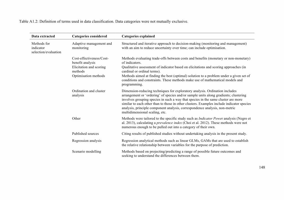
148

Table A1.2: Definition of terms used in data classification. Data categories were not mutually exclusive.

Data extracted Categories considered Categories explained Methods for indicator selection/evaluation

Adaptive management and monitoring

Structured and iterative approach to decision-making (monitoring and management) with an aim to reduce uncertainty over time; can include optimisation.

Cost-effectiveness/Cost-benefit analysis

Methods evaluating trade-offs between costs and benefits (monetary or non-monetary) of indicators.

Elicitation and scoring methods

Qualitative assessment of indicator based on elicitations and scoring approaches (in cardinal or ordinal terms).

Optimisation methods Methods aimed at finding the best (optimal) solution to a problem under a given set of conditions and constraints. These methods make use of mathematical models and programming.

Ordination and cluster analysis

Dimension-reducing techniques for exploratory analysis. Ordination includes arrangement or ‘ordering’ of species and/or sample units along gradients; clustering involves grouping species in such a way that species in the same cluster are more similar to each other than to those in other clusters. Examples include indicator species analysis, principle component analysis, correspondence analysis, non-metric multidimensional scaling, etc.

Other Methods were tailored to the specific study such as Indicator Power analysis (Negro et al. 2013), calculating a prevalence index (Choi et al. 2012). These methods were not numerous enough to be pulled out into a category of their own.

Published sources Citing results of published studies without undertaking analysis in the present study. Regression analysis Regression analytical methods such as linear GLMs, GAMs that are used to establish

the relative relationship between variables for the purpose of prediction. Scenario modelling Methods based on projecting/predicting a range of possible future outcomes and

seeking to understand the differences between them.

149

Table A1.2 cont. Data extracted Categories considered Categories explained Species accumulation/area

curves, Rarefaction curves Species represented/recorded as a function of cumulative monitoring effort (indicator).

Standard statistical tests Includes tests of statistical significance, e.g. t-test, chi-square, ANOVA, spatial and temporal correlations; and simple descriptive statistics. e.g. comparing means or box-plots for indicators.

Monitoring objectives (as used in Figure A1.2)

Complementarity Ability of indicator to provide information (e.g., on behavioural ecology, habitat use, or responses to management) that is complementary to the available information i.e. indicator contributes unrepresented values to an existing set of information (Tulloch et al. 2013).

Cost Objectives addressing cost of monitoring, analysis or dissemination of information. Feasibility Objectives addressing ease of monitoring, analysis or interpretation of indicator. Precision/accuracy Ability of the indicator to increase precision/accuracy of information. Sensitive to management Ability of indicator to detect change/effect due to management; commonly used in

management evaluation studies. Sensitive to pressures Ability of indicator to detect change due to explicitly stated natural

environmental/habitat conditions or natural or anthropogenic pressures; changes could be spatial, temporal, across environmental gradients or pressure intensities. Management is not included in this category.

Surrogacy Spatial or temporal representation of target state (other biodiversity, environmental conditions) when these are not under the influence of explicitly defined drivers of change.

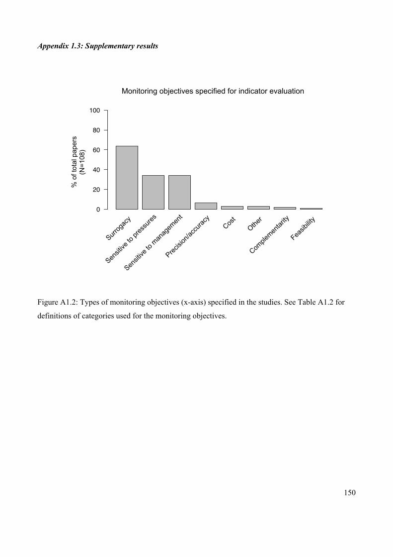
150

Appendix 1.3: Supplementary results

Figure A1.2: Types of monitoring objectives (x-axis) specified in the studies. See Table A1.2 for

definitions of categories used for the monitoring objectives.

Surro

gacy

Sens

itive

to p

ress

ures

Sens

itive

to m

anag

emen

t

Prec

ision

/acc

urac

y

Cost

Oth

er

Com

plem

enta

rity

Feas

ibilit

y

% o

f tot

al p

aper

s

0

20

40

60

80

100

Q.16 Types of monitoring objectives

% o

f tot

al p

aper

s (N

=108

) Monitoring objectives specified for indicator evaluation

151

Figure A1.3: Details of indicators species considered in the review.

Anim

al−r

elat

ed

Plan

t−re

late

d

Oth

er

% o

f tot

al p

aper

s

0

20

40

60

80

100

Q.5 Is the indicator plant or animal−related?

Spec

ies

Taxa

Com

mun

ity

Gui

ld

Spec

ies

of s

pecia

l con

cern

Oth

er

% o

f tot

al p

aper

s

0

20

40

60

80

100

Q.6 Type of indicator

Fiel

d m

easu

rem

ents

Data

base

Publ

ished

sou

rces

Sim

ulat

ions

or m

odel

ling

Elici

ted

from

exp

erts

Oth

er

% o

f tot

al p

aper

s

0

20

40

60

80

100

Q.7 How was data on indicator collected?

Spec

ies

dive

rsity

/iden

titie

s

Abun

danc

e or

den

sity

Pres

ence

/abs

ence

Dem

ogra

phic/

life h

istor

y tra

its

Oth

er

Rang

e/di

strib

utio

n

Perc

eive

d va

lue

Beha

viour

al a

spec

ts

Biom

ass,

size

Acou

stic

data

% o

f tot

al p

aper

s

0

20

40

60

80

100

Q.8 Type of data collected for the indicator

% o

f tot

al p

aper

s (N

=108

)

Animal or plant-related indicators Type of indicator

Type of data collected for the indicator Data collection method

% o

f tot

al p

aper

s (N

=108

)

152


Appendix 2.1: Parameter notation for VOI analysis

Table A2.1: Complete list of parameters and their notation used in the manuscript and in the

supporting information.

Variable Notation

Species index !

Threat index #

True model $

True state of decline/no decline due to threat i in species j in model s %&'(

Probability that threat i is causing a decline in species j )&'

Probability of species j declining *'

Background probability of decline in species j +'

Amount invested in managing threat i ,&

Total budget available for management -

Cost of eliminating threat # .&

Prior probability of model s Pr(s)

Expected number of species declining given model s and investment m1

in species 1 /( ,0

Observed state of decline/no decline in species j xj

Vector of responses (decline/no decline) for species j and k for each

experiment 1' 12

153

Appendix 2.2: Analytical solution to first term of EVPI equation

We found an analytical solution to the first term of the EVPI equation (equation 3.3) using

Lagrange minimisation (Bertsekas 1982). To solve the first term of the EVPI equation, we choose

the amount invested in managing threat 1 (,0) that minimises the expected number of species

declining while meeting the following constraints:

(a) ,0 ≥ 0 ensures that investment in threat 1 cannot be negative.

(b) ,0 ≤ .0 ensures that the amount invested in threat 1 cannot be greater than the cost of

eliminating threat 1, c1.

(c) ,0 ≤ - ensures the amount spent on threat 1 cannot be larger than the budget, B.

(d) - −,0 ≤ .8 ensures that the amount spent on threat 2 cannot be greater than the cost of

eliminating threat 2, c2.

An analytical solution can be obtained when the objective is to minimise the expected number of

species declining using Lagrange minimisation (Bertsekas 1982). To minimise /(,0) subject to

inequality constraints, we rewrite the constraints in the form ; ,0 ≥ 0:

1. ,0 ≥ 0

2. −,0 +.0 ≥ 0

3. - −,0 ≥ 0

4. ,0 − - + .8 ≥ 0

The Lagrangian can then be written as

= = / ,0 − ?0 constraint1 − ?8 constraint2 − ?I constraint3 − ?K constraint4

Eqn A2.1

where λ1, λ2 and λ3 and λ4 are arbitrary constants used in Lagrange minimisation called Lagrange

multipliers (Bertsekas 1982). Since the constraints are binding, i.e. the inequality constraint holds

with equality at the boundaries of the constraints, the simultaneous equations to be solved are:

?0 ,0 = 0, Eqn A2.2

?8 −,0 + .0 = 0, Eqn A2.3

?I - −,0 = 0, Eqn A2.4

?K ,0 + .8 − - = 0. Eqn A2.5

154

Then we set the derivative for the Lagrangian with respect to m1 to zero to obtain the minimum, MN

MOP= M

MOP/ ,0 − ?0 ,0 − ?8 −,0 + .0 − ?I - −,0 − ?K ,0 + .8 − - = 0

Eqn A2.6

Solving the equations A2.2, A2.3, A2.4, A2.5 and A2.6 for ,0, we get the following five solutions:

,0 =12

.8)0' − .0)8' + -)0')8' + .0)0')8' − .8)0')8')0')8'

I

'Q0

,

Eqn A2.7

,0 = 0, Eqn A2.8

,0 = -, Eqn A2.9

,0 = .0, and Eqn A2.10

,0 = - − .8. Eqn A2.11

Four of the five solutions are at the boundaries of the constraints, while one of the solutions is in the

interior. If the constraints do not hold for the interior solution then one of the solutions at the

boundary holds. The optimal solution is the one that results in lowest number of species declining

from the ones that satisfy the constraints. Solutions that break the constraints are ignored.

155

Appendix 2.3: EVSI formulation

EVSI equations at a glance

Monitoring one species under the non-experimental approach,

TUVW = − Pr Y' minOP

/( ,0

[K

(Q0

*\ $|Y'

0

^_Q`

+ minOP

/( ,0 *\ $

[K

(Q0

Eqn A2.12

where xj = 0 if species j is not declining and xj = 1 if species j is declining; Pr(xj) is the probability

of observing xj; and Pr(s|xj) is the probability that model s is the true model given xj has been

observed (i.e. the posterior probability).

We use Bayes Theorem to work out the posterior distribution for a specific model from the set of all

models, a ∈ c,as

Pr $ Y' = de Y' $ de (

de Y' f de ghijkP

Eqn A2.13

To solve for the above equation, we need to calculate *\ Y' $ . *\ Y' f is the same as *\ Y' $

where f represents all 64 models in set c and $ represents one particular model in set c . The

denominator in equation A2.13 sums over every possible model in c and gives the probability of

obtaining sample Y'.

Monitoring two species under the non-experimental approach,

TUVW = − Pr Y', Y2 minOP

/( ,0 *\ $|Y', Y2

[K

(Q0

0

^lQ`

0

^_Q`

+ minOP

/( ,0 *\ $

[K

(Q0

Eqn A2.14

where Pr Y', Y2 is the joint probability of observing the data for two species, j and k, and

*\ $|Y', Y2 is the probability that model s is the true model given Y'andY2 have been observed.

In the case of the experimental approach, the probability of the observed data is conditional on the

experiment conducted and the posterior model probabilities are conditional on the data and the

experiment.

156

When monitoring one species under the experimental approach,

TUVW = − Pr 1' minOP

/( ,0

[K

(Q0

*\ $|1'1_

+ minOP

/( ,0 *\ $

[K

(Q0

Eqn A2.15

where m'is a vector of responses for species j for each experiment of length equal to the number of

experiments, each entry is 1 if the species is declining and 0 if it is not and the sum is over all

possible combinations of the data.

When monitoring two species under the experimental approach,

TUVW = − Pr 1', 12 minOP

/( ,0

[K

(Q0

*\ $|1', 121l1_

+ minOP

/( ,0 *\ $

[K

(Q0

Eqn A2.16

where m' and m2 are two vectors of responses to each experiment for species j and k, respectively,

and *\ $|1', 12 is the probability that model s is the true model given that m' and m2 have been

observed.

A monitoring strategy comprised of selecting only species under the non-experimental approach as

opposed to selecting species and threat under the experimental approach. For example monitor

species A under no management of threats or monitor species A and B under management of threat

X, respectively. In all we compared eighteen monitoring strategies including:

(a) Monitoring one or two species under no management of threats (6 strategies)

(b) Monitoring one or two species under experimental management of threat 1 (6 strategies)

(c) Monitoring one or two species under experimental management of threat 2 (6 strategies).

Detailed derivation of EVSI equations

I. Non-experimental monitoring strategy

Let’s first consider a strategy where we only monitor one species with perfect detection, i.e. if the

species being monitored is declining we detect it without any error. In this case, the sample

information obtained from monitoring species !, Y' can take two values {0 or 1} indicating no

decline or decline in species, !. Since we assume binary links such that a threat either causes decline

157

or does not and a species declines even if only one of the threats causes a decline, we can write the

probability of the monitored species declining, given the model, $, as

Pr Y' = 1 $ = +' + 1 − +' max&∈0,8

%&'(() and

Pr Y' = 0 $ = 1 − +' + 1 − +' max&∈0,8

%&'(

where Y' is the sample information obtained from monitoring species, !, +' is the background

probability of decline for species j and %&'(() is the true state of decline/no decline due to threat i in

species j in model s such that %&'( = 0 if threat i does not cause a decline in species j in model s and

%&'( = 1if threat i causes a decline in species j in model s. Substituting terms in equation A2.12, we

get

Pr $ Y' = 1 =+' + 1 − +' max

&∈0,8%&'(() ×*\ $

+' + 1 − +' max&∈0,8

%&'(g) ×*\ f[K

gQ0

and

Pr $ Y' = 0 =+' + 1 − +' 1 − max

&∈0,8%&'( ×*\ $

1 − +' + 1 − +' max&∈0,8

%&'( ×*\ f[K

gQ0

.

We can also estimate probability of obtaining sample information, Y',

Pr Y' = 1 = *\ Y' = 1 $ Pr($)

[K

(Q0

= +' + 1 − +' max&∈0,8

%&'( ×*\ $

[K

(Q0

and

Pr Y' = 0 = 1 − Pr(Y' = 1).

As we now have all the components for the EVSI equation, we can estimate EVSI for a single

monitored species, ! under a non-experimental monitoring strategy (i.e. equation A2.12),

TUVW = − Pr Y' minOP

/( ,0

[K

(Q0

*\ $|Y'

0

^_Q`

+ minOP

/( ,0 *\ $

[K

(Q0

.

158

When monitoring two species, the joint probability of observing the sample from monitoring both

species, ! and a, in model $, is the product of the individual probabilities, assuming they are

independent. Therefore,

Pr Y' = 0, Y' = 0 $ = Pr Y' = 0 $ ×Pr Y2 = 0 $

= 1 − +' + 1 − +' max&∈0,8

%&'( ×1 − +2 + 1 − +2 max

&∈0,8%&2( ,

Pr Y' = 0, Y2 = 1 $ = Pr Y' = 0 $ ×Pr Y2 = 1 $

= 1 − +' + 1 − +' max&∈0,8

%&'( ×+2 + 1 − +2 max

&∈0,8%&2( ,

Pr Y' = 1, Y2 = 0 $ = Pr Y' = 1 $ ×Pr Y2 = 0 $

= +' + 1 − +' max&∈0,8

%&'(() ×1 − +2 + 1 − +2 max

&∈0,8%&2( , and

Pr Y' = 1, Y2 = 1 $ = Pr Y' = 1 $ ×Pr Y2 = 1 $

= +' + 1 − +' max&∈0,8

%&'(() ×+2 + 1 − +2 max

2∈0,8%&2(() ,

where Y' and Y2is the sample information obtained from monitoring species ! and a individually.

Model posterior probabilities are estimated as before, using Bayes Theorem (equation A2.13)

Pr $ Y', Y2 = Pr Y', Y2 $ Pr $

Pr Y', Y2 f Pr f[KgQ0

.

For example,

Pr $ Y' = 1, Y2 = 0

=Pr Y' = 1 $ ×Pr Y2 = 0 $ ×*\ $

Pr Y' = 1 f ×Pr Y2 = 0 f ×*\ f[KgQ0

=

+' + 1 − +' max&∈0,8

%&'( × 1 − +2 + 1 − +2 max

&∈0,8%&2(

×*\ $

+' + 1 − +' max&∈0,8

%&'g × 1 − +2 + 1 − +2 max

&∈0,8%&2g

×*\ f

[KgQ0

.

We can write the expressions for the other three events similarly i.e. for Pr $ Y' = 0, Y2 = 1 ,

Pr $ Y' = 1, Y2 = 0 and Pr a Y' = 0, Y2 = 0 .

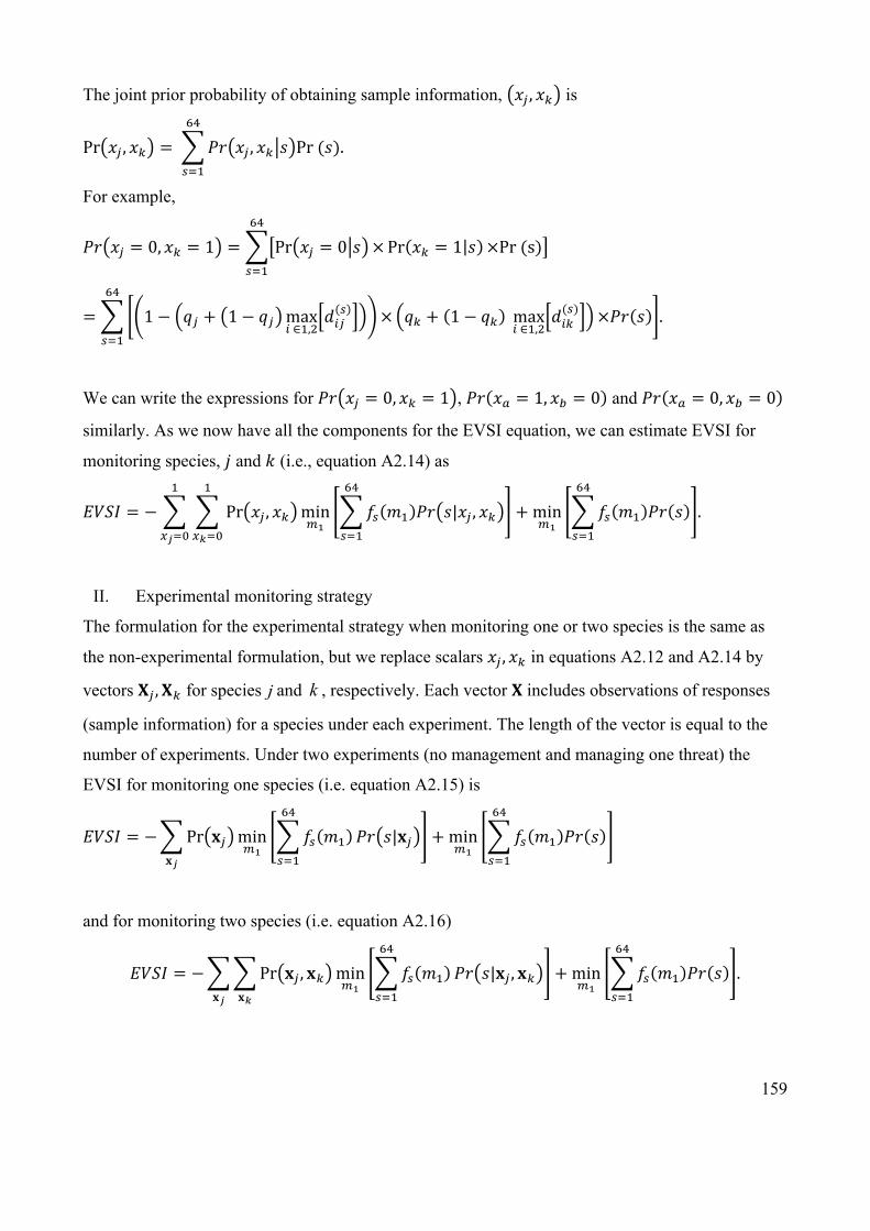
159

The joint prior probability of obtaining sample information, Y', Y2 is

Pr Y', Y2 = *\ Y', Y2 $ Pr($)

[K

(Q0

.

For example,

*\ Y' = 0, Y2 = 1 = Pr Y' = 0 $ ×Pr Y2 = 1 $ ×Pr(s)

[K

(Q0

= 1 − +' + 1 − +' max&∈0,8

%&'( × +2 + 1 − +2 max

&∈0,8%&2(() ×*\ $

[K

(Q0

.

We can write the expressions for *\ Y' = 0, Y2 = 1 , *\ Yq = 1, Yr = 0 and *\ Yq = 0, Yr = 0

similarly. As we now have all the components for the EVSI equation, we can estimate EVSI for

monitoring species, ! and a (i.e., equation A2.14) as

TUVW = − Pr Y', Y2 minOP

/( ,0 *\ $|Y', Y2

[K

(Q0

0

^lQ`

0

^_Q`

+ minOP

/( ,0 *\ $

[K

(Q0

.

II. Experimental monitoring strategy

The formulation for the experimental strategy when monitoring one or two species is the same as

the non-experimental formulation, but we replace scalars Y', Y2 in equations A2.12 and A2.14 by

vectors m', m2 for species and , respectively. Each vector m includes observations of responses

(sample information) for a species under each experiment. The length of the vector is equal to the

number of experiments. Under two experiments (no management and managing one threat) the

EVSI for monitoring one species (i.e. equation A2.15) is

TUVW = − Pr 1' minOP

/( ,0

[K

(Q0

*\ $|1'1_

+ minOP

/( ,0 *\ $

[K

(Q0

and for monitoring two species (i.e. equation A2.16)

TUVW = − Pr 1', 12 minOP

/( ,0

[K

(Q0

*\ $|1', 121l1_

+ minOP

/( ,0 *\ $

[K

(Q0

.

j k

160

Appendix 2.4: Case study details

VOI formulation for Fitz-Stirling case study

For the model system, the expected number of species declining under management (equation 3.4)

is expressed as

/( ,0 = +' + 1 − +' 1 − 1 − %0'(() .0 − ,0

.01 − %8'

(() .8 − ,8

.8

I

'Q0

when all species decline in response to the two threats present in the system. The fox-fire case study

is a special case of this model, wherein one of the species (tammar wallaby) does not decline in

response to one of the threats (fire). Instead, the wallaby benefits from fires because of the

regeneration of grasses and fruiting shrubs following a fire providing replenished food stocks

(Christensen 1980). As a result fire is not a threat for the wallaby. Instead, the management of fire

to reduce fire intensity can cause a decline in wallaby abundance. Therefore, for the wallaby, %&',

where # indicates fire threat, represents the state of decline or no decline (1 or 0) when fire threat is

managed. And the expected number of species decline is be re-written as

= +' + 1 − +' 1 − 1 − %0'( .0 − ,0

.01 − %8'

(() .8 − ,8

.8

8

'Q0

+ +s + 1 − +s 1 − 1 − %0s( .0 − ,0

.0%8s( − %8s

( .8 − ,8

.8

Eqn A2.17

where ! = {1,2} represents the bandicoot and the brushtail possum, while +s, %0s( and%8s

( are the

probability of decline for the wallaby due to unknown factors, and the state of decline due to foxes

and fires, respectively.

For the brushtail possum and the bandicoot, we assume that managing a threat reduces the

probability of the threat causing a decline to zero. We calculated the )&' and +' values for the three

species included in the case study based on data described in Tulloch, Chadès and Possingham

(2013). So if we manage threat 1 then )0' = 0 and Pr decline managedthreat1 = +' +

1 − +' )8'.

161

We then estimated the probability of the threats individually causing a decline as

)8' =de z{|}~�{|ÄÅ�ÅÇ{zÉÑe{ÅÉ0 ÖÜ_

0ÖÜ_and )0' =

de z{|}~�{|ÄÅ�ÅÇ{zÉÑe{ÅÉ8 ÖÜ_0ÖÜ_

.

If we manage both threats we can estimate the background probability of decline, due to extrinsic or

intrinsic factors other than the two threats causing decline (Cardillo et al. 2008; Di Marco et al.

2012) as +' = *\ decline|managedboththreats .

For the tammar wallaby however, fire is not a threat and managing fire introduces the threat,

causing the species to decline. Therefore, we treat fire differently in this case such that decline due

to fire %8s occurs when foxes are managed and fire is also managed (because managing fire

introduces the threat) and decline due to foxes %0s occurs when fire is not managed and foxes are

not managed. If +s is the probability of decline when foxes are managed but fire is not managed,

+s = *\ decline|managedthreat1andNOTmanagedthreat2 .

The associated probabilities can be written as

)8s =Pr decline|managedthreat1andmanagedthreat2 − +'

1 − +' , and

)0s =Pr decline|NOTmanagedthreat1andNOTmanagedthreat2 − +'

1 − +'.

Parameter estimation for Fitz-Stirling case study

I. Probability of species decline under management

We estimated the probability of species declines under management based on data described in

Tulloch, Chadès and Possingham (2013). Time-series from the candidate indicator under a given

action are combined into a dataset of length n, with one population growth rate value (µ) per

generation, and growth rate variability ãå. We define the likelihood that the observed growth rate µ

is greater than a given growth rate threshold x as *& ç > Y ,

*& ç > Y = 1 − *& ç ≤ Y Eqn A2.18

*& ç ≤ Y = è Y − çå ãå ê Eqn A2.19

where Φ represents the cumulative distribution function of the standard normal and x can be any

target growth rate set by the user. For example, the probability of observing any increase in

162

population size is given by *& ç > 0 . The ‘true’ growth rate çå and x are scaled logarithmically;

with çå calculated as the mean of all the recorded growth rates (µ) from the accumulated time-

series dataset of length n for each species. The chance of observing a real growth rate, *& ç > 0 ,

increases with increasing data availability n and decreasing variability (σ) of growth rates (µ).

Equation A2.19 determines the probability of an observed growth rate being less than a given target

growth rate x, formally noted *& ç ≤ Y , and referred to as *& Y from here on. See Tulloch,

Chadès and Possingham (2013) for full details on probability estimation.

II. Cost of managing threats

We estimated the cost of a one-year fox-baiting management program for a typical 25km2

vegetation patch in the Fitz-Stirling (Tulloch et al. 2016a). We considered three factors: number of

baiting events required, travel cost and operation costs. We considered baiting 12 times per year for

optimal baiting frequency. Average cost of travel from the nearest major town was $225.81

(Auerbach, Tulloch & Possingham 2014; Evans et al. 2015) and annual cost of ground-delivered

fox baiting, for baiting 4 times a year to reflect conservation agencies’ average management

expenditure in the region, was $100 per km2 (Tulloch et al. 2014).

Totalcostoffoxmanagementforayear

= Numberofbaitingevents×Travelcostbyroad +

Operationcostperkm×Areaofmanagement

= 12× $225.81 + $1004

×25km8 = $10209.72perkm8.

Similarly, Evans et al. (2015) estimate the operation cost of fire management by ground burning a

small part of the habitat to ensure the remainder stays unburnt as $11250 per unit, where a unit is a

defined management area that can be feasibly managed in a single day. We considered managed

burning twice in a year for a highly connected habitat patch in the Fitz-Stirling. 90% of the remnant

habitat patches between the Stirling Range and Fitzgerald River National Parks are small (average

area ~2km2) and unconnected with low wildfire risk, requiring periodic management burning only

once every 40 to 80 years to reduce the chance of senescence of fire-dependent plants such as

Banksia (Tulloch et al. in press). The majority (83%) of the area of remnant vegetation in this

region is within larger highly connected patches at least 15km2 in area. It is these patches we chose

for the study as they have a higher likelihood of containing the target mammals due to having a

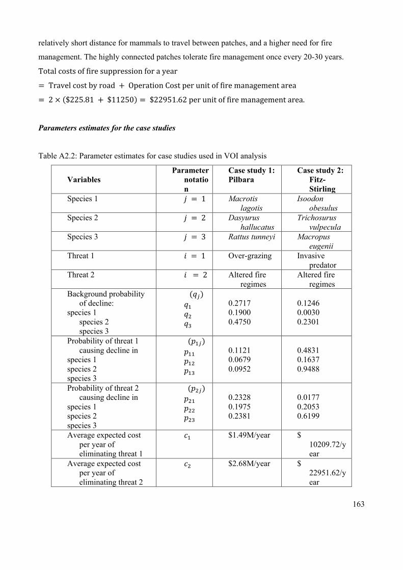
163

relatively short distance for mammals to travel between patches, and a higher need for fire

management. The highly connected patches tolerate fire management once every 20-30 years.

Totalcostsoffiresuppressionforayear

= Travelcostbyroad + OperationCostperunitoffiremanagementarea

= 2× $225.81 + $11250 = $22951.62perunitoffiremanagementarea.

Parameters estimates for the case studies

Table A2.2: Parameter estimates for case studies used in VOI analysis

Variables Parameter

notation

Case study 1: Pilbara

Case study 2: Fitz-Stirling

Species 1 ! = 1 Macrotis lagotis

Isoodon obesulus

Species 2 ! = 2 Dasyurus hallucatus

Trichosurus vulpecula

Species 3 ! = 3 Rattus tunneyi Macropus eugenii

Threat 1 # = 1 Over-grazing Invasive predator

Threat 2 # = 2 Altered fire regimes

Altered fire regimes

Background probability of decline:

species 1 species 2 species 3

(+')+0+8+I

0.2717 0.1900 0.4750

0.1246 0.0030 0.2301

Probability of threat 1 causing decline in


()0'))00)08)0I

0.1121 0.0679 0.0952

0.4831 0.1637 0.9488

Probability of threat 2 causing decline in


()8'))80)88)8I

0.2328 0.1975 0.2381

0.0177 0.2053 0.6199

Average expected cost per year of eliminating threat 1

.0 $1.49M/year $ 10209.72/year

Average expected cost per year of eliminating threat 2

.8 $2.68M/year $ 22951.62/year

164


Figure A2.1: VOI sensitivity to decision-making scenarios. VOI is expressed as the reduction in

expected number of species declining (i.e. for best monitoring strategy). Relative budget (x-axis),

expressed as a percentage of the total budget required to completely manage both threats. Threat

probabilities (y-axis) i.e. probability of both threats causing declines in all species increases from 0

to 1 (scenario 1); relative probability of threat 1 causing declines in all three species increases from

0 to 1 and relative probability of threat 2 causing decline in all three species decreasing from 1 to 0

(scenario 2); probability of both threats causing declines increases from 0 to 1 for species 1,

decreases from 1 to 0 for species 3 and is fixed at 0.5 for species 2 (scenario 3). Scenarios are tested

at fixed cost of eliminating threats (each costing 50% of total budget) and low background

probability of decline (0.01).

00.20.40.60.81

00.20.40.60.81

0 50 1000

0.20.40.60.81

0 50 1000 50 100

0

0.1

0.2

0.3

0.4

0 0.1 0.2 0.3 0.4

EVPI EVSI

(Experimental, 1 species monitoring)

EVSI (Experimental,

2 species monitoring)

EVPI/EVSI

Thre

at p

roba

bilit

ies

For a

ll th

reat

s Fo

r thr

eat 1

Fo

r spe

cies

1

Relative budget




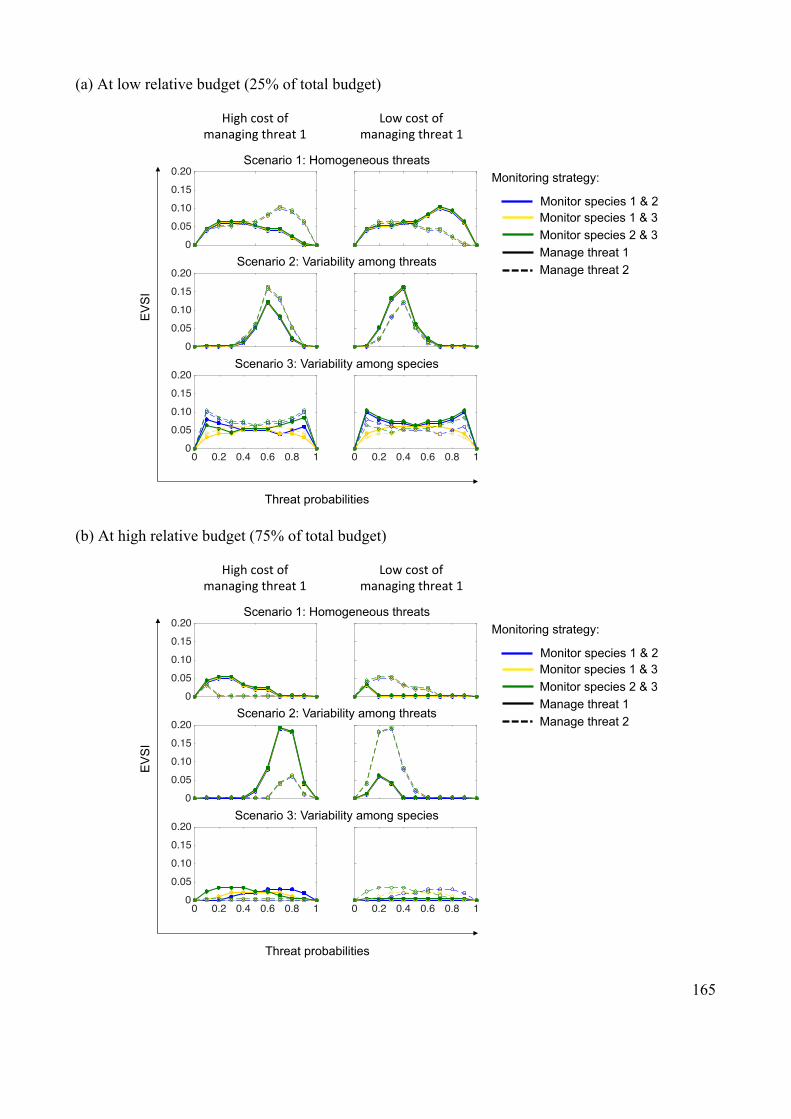
165

(a) At low relative budget (25% of total budget)

(b) At high relative budget (75% of total budget)

0

0.05

0.10

0.15

0.20

0

0.05

0.10

0.15

0.20

0 0.2 0.4 0.6 0.8 10

0.05

0.10

0.15

0.20

0 0.2 0.4 0.6 0.8 1


EV

SI





Monitoring strategy:

@ low budget (25%)




0

0.05

0.10

0.15

0.20

0

0.05

0.10

0.15

0.20

0 0.2 0.4 0.6 0.8 10

0.05

0.10

0.15

0.20

0 0.2 0.4 0.6 0.8 1


EV

SI





Monitoring strategy:

@ high budget (75%)




166

Figure A2.2 (previous page): Performance of two species experimental monitoring strategies at (a)

low relative budget (25 % of total budget required to completely manage both threats) and (b) high

relative budget (75 % of total budget required to completely manage both threats). Coloured lines

indicate which species was/were monitored (as per legend). Solid lines indicate that the species

was/were monitored under experimental management of threat 1 and dotted lines indicate that the

species was/were monitored under experimental management of threat 2. EVSI (y-axis) is

expressed as the reduction in expected number of species declining. Threat probabilities (x-axis) i.e.

probability of both threats causing declines in all species increases from 0 to 1 (scenario 1); relative

probability of threat 1 causing declines in all three species increases from 0 to 1 and relative

probability of threat 2 causing decline in all three species decreasing from 1 to 0 (scenario 2);

probability of both threats causing declines increases from 0 to 1 for species 1, decreases from 1 to

0 for species 3 and is fixed at 0.5 for species 2 (scenario 3). Blue, yellow and green strategies

overlapping in scenarios 1 and 2 while in scenario 3, only strategies close to zero are overlapping.

Scenarios tested at low background probability of decline (0.01), and fixed relative cost of

managing threat 1 (as specified in figure).

Figure A2.3 (next page): Case study results: (a) Pilbara and (b) Fitz-Stirling. EVSI (y-axis) is

expressed as the reduction in expected number of species declining. Coloured lines indicate which

species was/were monitored (as per legend). Solid lines indicate that the species was/were

monitored under experimental management of threat 1 and dotted lines indicate that the species

was/were monitored under experimental management of threat 2. Relative budget (x-axis),

expressed as a percentage of the total budget required to completely manage both threats. Overall

EVSI is higher in the Pilbara because of high relative cost of managing the threat with high threat

probability (altered fire regimes) as compared to the Fitz-Stirling with low relative cost of

managing the threat with high threat probability (invasive predator). However, maximum EVSI in

both cases is low (maximum EVSI = 0.06) due to the high values of background probability of

decline.

167

(a) Pilbara case study results

(b) Fitz-Stirling case study results

0 50 1000

0.02

0.04

0.06

0 50 1000

0.02

0.04

0.06

0 50 1000

0.02

0.04

0.06

0 50 1000

0.02

0.04

0.06

EV

SI

One

spe

cies

Tw

o sp

ecie

s

Passive monitoring Experimental monitoring

Relative budget

Pilbara'

Manage grazing Manage fire

Monitor M.lagotis Monitor D.hallucatus Monitor R.tunneyi

Monitoring one species:

Manage grazing Manage fire

Monitor M.lagotis & D.hallucatus Monitor M.lagotis & R.tunneyi Monitor D.hallucatus & R.tunneyi

Monitoring two species:

0 50 1000

0.02

0.04

0.06

0 50 1000

0.02

0.04

0.06

0 50 1000

0.02

0.04

0.06

0 50 1000

0.02

0.04

0.06

EV

SI

One

spe

cies

Tw

o sp

ecie

s

Relative budget

Fitz%Sterling,

Manage foxes Manage fire

Monitor I.obesulus Monitor T.vulpecula Monitor M.eugenii

Monitoring one species:

Manage foxes Manage fire

Monitor I.obesulus & T.vulpecula Monitor I.obesulus & M.eugenii Monitor T.vulpecula & M.eugenii

Monitoring two species:

Passive monitoring Experimental monitoring

168

Appendix 2.6: MATLAB code for VOI analysis

Readers interested in replicating our approach can download the MATLAB code (MATLAB

Version R2015b (Mathworks 1984–2015)) used in our study from the link provided below. Please

send an email to lead author to enquire about updated versions of the code.

Link to MATLAB code:

https://dl.dropboxusercontent.com/u/16805473/Bal%20et%20al_MATLAB%20code.zip

References for Appendix 2

Auerbach, N.A., Tulloch, A.I.T. & Possingham, H.P. (2014) Informed actions: where to cost effectively manage multiple threats to species to maximize return on investment. Ecological Applications, 24, 1357-1373.

Bertsekas, D.P. (1982) Constrained optimization and Lagrange multiplier methods. Academic Press, New York.

Cardillo, M., Mace, G.M., Gittleman, J.L., Jones, K.E., Bielby, J. & Purvis, A. (2008) The predictability of extinction: biological and external correlates of decline in mammals. Proceedings of the Royal Society of London B: Biological Sciences, 275, 1441-1448.

Christensen, P.E.S. (1980) The biology of Bettongia penicillata (Gray, 1837), and Macropus eugenii (Desmarest, 1812) in relation to fire in Western Australia. pp. 1-90. Bulletin, Forests Department, Western Australia.

Di Marco, M., Cardillo, M., Possingham, H.P., Wilson, K.A., Blomberg, S.P., Boitani, L. & Rondinini, C. (2012) A novel approach for global mammal extinction risk reduction. Conservation Letters, 5, 134-141.

Evans, M.C., Tulloch, A.I.T., Law, E.A., Raiter, K.G., Possingham, H.P. & Wilson, K.A. (2015) Clear consideration of costs, condition and conservation benefits yields better planning outcomes. Biological Conservation, 191, 716-727.

Tulloch, A.I.T., Chadès, I. & Possingham, H.P. (2013) Accounting for Complementarity to Maximize Monitoring Power for Species Management. Conservation Biology, 27, 988-999.

Tulloch, A.I.T., Pichancourt, J.-B., Gosper, C.R., Sanders, A. & Chadès, I. (2016) Fire management strategies to maintain species population processes in a fragmented landscape of fire-interval extremes. Ecological Applications.

169


Appendix 3.1: Parameter notation used in the VOI analysis

Table A3.1: Parameter notation used in the VOI analysis

Variable Notation

Threat index #

Species index j

Time step ü

Abundance of species at time t †°

Growth rate of species in the absence of management \

Change in growth rate of species per unit of investment in managing

threat i ¢&

Rate of increase of population abundance ?

Investment in managing threat i ,&

Total budget available for management -

Expected benefit of managing threat i (i.e. mean of ¢&) µi

Uncertainty in benefit of managing threat i (i.e. variance of ¢&) σ2i

Difference in expected benefit of managing the two threats, ç0 − ç8 w

170

Appendix 3.2: Detailed derivation of the EVPI and EVXI equations

Finding the optimal solution under no uncertainty

For the objective function,

U ,0,,8 = \ + ¢0,0 + ¢8,8 + fê †° Eqn A3.1

since,8 = - −,0, the optimisation problem becomes finding the value of m1 that maximises

equation A3.1. Assuming Nt and r are constants such that £ = \ + fê †° ,

maxOP

U ,0 = maxOP

£ + ¢0,0 + ¢8 - −,0

= £ +maxOP

¢0,0 + ¢8 - −,0 .

Eqn A3.2

Since ¢0,0 + ¢8 - −,0 is a linear function m1, the optimal solution will always be at one of the

extremes. If ¢0and ¢8 are known and ¢0 > ¢8, it is optimal to let m1 = B; and if ¢0 < ¢8, it is

optimal to let m1 = 0. Therefore,

maxOP

¢0,0 + ¢8 - −,0 = -max ¢0, ¢8 .

Eqn A3.3

The maximum of two variables on the right hand side of equation A3.3 can be found as (Moore et

al. in review1)

maxOP

¢0,0 + ¢8 - −,0 =-2 ¢0 + ¢8 + ¢0 − ¢8 .

Eqn A3.4

Therefore, under perfect information the value of the optimal management function is

maxOP

U ,0 = £ +-2¢0 + ¢8 + ¢0 − ¢8 .

Eqn A3.5

1 Moore AL, Walker L, Runge MC, McDonald-Madden E & McCarthy MA (in review) Two-step adaptive

management for choosing between two management actions. https://mickresearch.wordpress.com/2016/07/05/simple-

adaptive-management/

171

Expected value of perfect information (EVPI)

Now assume there is uncertainty in the βs such that βi is normally distributed with mean µi and

variance σ2i. To calculate the value of perfect information,

TU*W = • maxOP

U ,0 − maxOP

• U ,0 .

Eqn A3.6

From equation A3.5, we note that

maxOP

• U ,0 = £ +-2ç0 + ç8 + ç0 − ç8 and

Eqn A3.7

• maxOP

U ,0 = £ +-2• ¢0 + • ¢8 + • ¢0 − ¢8 .

Eqn A3.8

Since the absolute value of a normally distributed random variable is a folded normally distributed

variable, the mean of ¢0 − ¢8 can be represented as

• ¢0 − ¢8 = −Y/ Y %Y

`

Ö¶

+ Y/ Y %Y

¶

`

where Y = ¢0 − ¢8 . Therefore,

• ¢0 − ¢8 =2 ã0

8 + ã88

ß®Ö ©PÖ©™ ™/ 8 ¨P

™≠¨™™− ç0 − ç8 ®\/

− ç0 − ç82 ã0

8 + ã88

.

Eqn A3.9

Let ç = • ¢0 − ¢8 , Æ = ç0 − ç8, and Ø = ã08 + ã88. Therefore,

TU*W = £ +-2• ¢0 + • ¢8 + • ¢0 − ¢8 − £ +

-2ç0 + ç8 + ç0 − ç8

= £ +-2ç0 + ç8 +

-2ç − £ −

-2ç0 + ç8 −

-2Æ

=-2ç − Æ

Eqn A3.10

and

ç = Ø2ß®Ös™

8∞™ − Æerf−Æ

Ø 2.

Eqn A3.11

172

Expected value of partial information (EVXI)

We consider observing the effect of one out of the two the management actions (tied to managing a

specific threat), therefore reducing the overall uncertainty (i.e. variance). If we can perfectly

monitor β1, then

TU±W≤0 = •≤P maxOP

•≤™ U ,0 − maxOP

•≤P,≤™ U ,0

Eqn A3.12

where •≥Pis the expectation taken over the distribution of the β1s after monitoring, •≥P,≥™ is the

expectation taken over the prior distribution of the βis before monitoring and •≥™is the expectation

taken over the prior distribution of the unmonitored β2. To calculate the first term,

•≤P maxOP

•≤™ U ,0 = •≤P maxOP

•≤™ £ + -max ¢0, ¢8

= £ + -•≤P maxOP

¢0, • ¢8

= £ + -•≤P maxOP

¢0, ç8

= £ +-2•≤P ¢0 + ç8 + ¢0 − ç8

= £ +-2 ç0 + ç8 + •≤P ¢0 − ç8

Eqn A3.13

Since ¢0 is observed and therefore constant, ¢0 − ç8~† ç0 − ç8, ã08 , ¢0 − ç8 is folded normal

with mean,

• ¢0 − ç8 =2 ã0

8

ß®Ö ©PÖ©™ ™

8 ¨P™− ç0 − ç8 ®\/

− ç0 − ç82 ã0

8

Eqn A3.14

Let • ¢0 − ç8 = ç≤0 and Æ = ç0 − ç8. The second term of the EVXI equation is the same as

that in the EVPI equation, therefore

TU±W≤0 = £ +-2ç0 + ç8 + •≤P ¢0 − ç8 − £ +

-2ç0 + ç8 + ç0 − ç8

= £ +-2ç0 + ç8 +

-2ç≤0 − £ −

-2ç0 + ç8 −

-2Æ

=-2ç≤0 − Æ

Eqn A3.15

173

and

ç≤0 = ã02ß®Ös™

8¨P™ − Æerf−Æ

ã0 2.

Eqn A3.16

Similarly, if we can perfectly monitor β2, then

TU±W≤8 = •≤™ maxOP

•≤P U ,0 − maxOP

•≤P,≤™ U ,0

Eqn A3.17

where •≥Pis the expectation taken over the prior distribution of β1, •≥P,≥™ is the expectation taken

over the prior distribution of the βis and •≥™is the expectation taken over the prior distribution of β2.

The expected benefit after resolving all uncertainty regarding β1 is

•≤™ maxOP

•≤P U ,0 = £ +-2 ç0 + ç8 + •≤™ ç0 − ¢8

Eqn A3.18

Since ¢8 is observed and therefore constant, ç0 − ¢8~† ç0 − ç8, ã88 , ç0 − ¢8 is folded normal

with mean,

• ç0 − ¢8 =2 ã8

8

ß®Ö ©PÖ©™ ™

8 ¨™™− ç0 − ç8 ®\/

− ç0 − ç82 ã8

8

Eqn A3.19

Let • ç0 − ¢8 = ç≤8 and Æ = ç0 − ç8. The second term of EVXI equation is the same as that in

the EVPI equation, therefore

TU±W≤8 =-2ç≤8 − Æ

Eqn A3.20

and

ç≤8 = ã82ß®Ös™

8¨™™ − Æerf−Æ

ã8 2.

Eqn A3.21

174

Appendix 3.3: Difference in EVXI for monitoring the effect of management on the threats

Using equations A3.15 and A3.20, we can write the difference in EVXI for monitoring the effect of

management on the threats i.e. for observing ¢0 and ¢8 as

TU±W≤0 − TU±W≤8 =-2ç≤0 − Æ −

-2ç≤8 − Æ

=-2ç≤0 − ç≤™

Eqn A3.22

Substituting expression for ç≤0 and ç≤8 from equations A3.16 and A3.21 in the above equation, we

get,

TU±W≤0 − TU±W≤8

=-2

ã02ß®Ös™


ã0 2− ã8

2ß®Ös™

8¨™™ − Æerf−Æ

ã8 2

Eqn A3.23

where B is the total budget available for management, w is the difference in expected benefit of

managing the two threats (i.e. µ1 – µ2), σ1 is a measure of the uncertainty in benefit of managing

threat 1 (i.e. the standard deviation of β1) and σ2 is a measure of the uncertainty in benefit of

managing threat 2 (i.e. the standard deviation of β2).

If σ12 = σ1

2 = σ2, then equation A3.23 can be rewritten as

TU±W≤0 − TU±W≤8 =-2

ã2ß®Ös™

8¨™ − Æerf−Æ

ã 2− ã

2ß®Ös™

8¨™ − Æerf−Æ

ã 2

=-20 = 0.

Eqn A3.24

Therefore, we can see that the difference in the EVXI for monitoring the effect of management on

the threats will always be zero when the uncertainty in the benefit of managing threat 1 (σ12) is

equal to the uncertainty in the benefit of managing threat 2 (σ22).

175

Table A3. 2: Range of values used to evaluate equation A3.32 (equation 4.15 in the chapter)

Parameters Range used

Budget available for management (B) Fixed at 10

Difference in expected benefit of managing the two threats (w) 0 to ± 5

Uncertainty in benefit of managing threat 1 (σ12) 0 to 5

Uncertainty in benefit of managing threat 2 (σ22) 0 to 5

Table A3.3: Monitoring strategies based on difference in EVXI for monitoring the effect of

management of threat 1 and threat 2, i.e. EVXIβ1 and EVXIβ2, respectively.

EVXI difference

Condition 1 Condition 2 Monitoring strategy*

Zero or close

to zero

| EVXIβ1 - EVXIβ2 |

≤ δ1

EVXIβ1, EVXIβ2 <

δ2 Do not monitor

Zero or close

to zero

| EVXIβ1 - EVXIβ2 |

≤ δ1 EVXIβ1, EVXIβ2 ≥ δ2

Monitor either of

the two threats

Positive EVXIβ1 - EVXIβ2 >

δ1 EVXIβ1 ≥ δ2

Monitor threat 1

only

Negative EVXIβ2 - EVXIβ1 >

δ1 EVXIβ2 ≥ δ2

Monitor threat 2

only

δ1 and δ1 values are arbitrary. δ1= 0.0001; δ2=0.01

δ1 was specified to classify EVXI difference values within a certain distance of zero as zero. δ2 was

specified to classify low EVXI values.

* By ‘monitor threat’ we mean monitor the effect of managing the threat.

176

Appendix 3.4: Detailed VOI formulation for the n-species, 2-threat system

To include multiple species, such that ! ∈ 1,2, . . ê that are potentially impacted by two threats,

# ∈ 1,2 , we model species population dynamics using a geometric growth model assuming

constant growth rate,

†',°≠0 = ?'†',°

Eqn A3.25

where Nj,t and Nj,t+1 are total abundances for species j at times t and t + 1. λj is the growth rate for

species j, such that

?' = ®µ_≠≤P_OP≠≤™_O™

Eqn A3.26

where βij is the change in growth rate of species j per unit of investment in managing threat i, mi is

the investment in managing threat i and rj is the growth rate of species j in the absence of threat

management. Assuming that the management objective is to maximise abundance of n species, we

specify the objective function as the log of the expected geometric mean population abundance, to

obtain a linear sum of terms, and sought to maximize the geometric mean:

; ,0,,8 = †',°≠0

å

'Q0

0 å

= ?'†',°

å

'Q0

0 å

= ®µ_≠≤P_OP≠≤™_O™†',°

å

'Q0

0 å

.

Eqn A3.27

Let fê ; ,0,,8 = U ,0,,8 , then we can write equation A3.27 in log form such that,

U ,0,,8 =\' + ¢0',0 + ¢8',8 + fê †',°

ê

å

'Q0

Eqn A3.28

177

Finding the optimal solution under no uncertainty

Since,8 = - −,0, the optimisation problem becomes finding the value of m1 that maximises the

above equation,

maxOP

U ,0 =1ê

\' + fê †',°

å

'Q0

+ maxOP

¢0',0 + ¢8' - − ,0

å

'Q0

= - \' + fê †',°

å

'Q0

+12

¢0'

å

'Q0

+12

¢8'

å

'Q0

+12

¢0'

å

'Q0

− ¢8'

å

'Q0

.

Eqn A3.29

Let £ = \' + fê †',°å'Q0 and ¢& = ¢&'

å'Q0 such that ¢& is the sum of the change in growth rate

per unit of investment in managing threat i across all species. As in case of the one-species, two-

threat model, ¢& is normally distributed with mean, ç& = ç&'å'Q0 and variance, ã&8 = ã&'

8å'Q0 .

Therefore,

maxOP

U ,0 =1ê£ +

-2¢0 + ¢8 + ¢0 − ¢8 .

Eqn A3.30

Subsequent EVPI and EVXI can be derived using the method detailed in appendix 3.2:

TU*W = -2ê

ç − Æ

Eqn A3.31

where

ç =2 ã0

8 + ã88

ß®Ö

©PÖ©™ ™

8 ¨P™≠¨™

™− ç0 − ç8 ®\/

− ç0 − ç82 ã0

8 + ã88

.

Eqn A3.32

When monitoring β1 perfectly,

TU±W≤0 = -2ê

ç≤0 − Æ

Eqn A3.33

where

ç≤0 =2 ã0

8

ß®Ö ©PÖ©™ ™

8 ¨P™− ç0 − ç8 ®\/

− ç0 − ç82 ã0

8.

Eqn A3.34

178

Appendix 3.5: Monitoring subset of species

If we perfectly monitor the effect of managing threat 1 on a subset of species, then let us assume

that we observe some of the βs perfectly such that

∂∑ = ¢0'

g

'Q0

Eqn A3.35

where ∂∑is the sum of the observed β1s and l is the number of species β1 is observed for. Similarly,

∂∏ = ¢0'

å

'Qg≠0

Eqn A3.36

where ∂∏ is the sum of the unobserved β1s. We order the species for which β is observed as ! ∈

1, . . f followed by the species for which β is not observed as ! ∈ f + 1, . . ê . Therefore,

TU*±W = •rπ maxOP

• rP rπ ,r™ U ,0 − maxOP

•rP,r™ U ,0

Eqn A3.37

where •rπ is the expectation taken over the distribution of the β1s after monitoring (averaged over

all possible observations for ¢0,0. . ¢0,g), •rP,r™ is the expectation taken over the prior distribution of

the βis before monitoring. • rP rπ ,r™is the expectation taken over the posterior distribution of the

monitored β1s and the prior distribution of the unmonitored β2s, given we have observed the true

values of the observed β1s.

Let ∂∑be normally distributed with mean ç∑ and variance ã∑8 ; and ∂∏be normally distributed with

mean ç∏ and variance ã∏8 such that ç∑ = ç0'g'Q0 andã∑

8 = ã0'8g

'Q0 ; and ç∏ =

ç0'å'Qg≠0 andã∏

8 = ã0'8å

'Qg≠0 .

179

To calculate the first term of the EVXI equation

maxOP

• rP rπ ,r™ U ,0 =£ê+-2ê

∂∑ + • ∂∏ + • ∂8 + • ∂∑ + ∂∏ − ∂8

=£ê+-2ê

∂∑ + ç∏ + ç8 + • ∂∑ + ∂∏ − ∂8

Eqn A3.38

where • ∂∑ = ç∑. Since ∂∑ + ∂∏ − ∂8~† ∂∑ + ç∏ − ç8, ã∏8 + ã8

8 , ∂∑ + ∂∏ − ∂8 is folded

normal with mean,

ç ∂∑ =2 ã∏

8 + ã88

ß®Ö rπ≠©ªÖ©™ ™

8 ¨ª™≠¨™

™− ∂∑ + ç∏ − ç8 ®\/

− ∂∑ + ç∏ − ç8 8

2 ã∏8 + ã8

8 .

Eqn A3.39

Therefore,

•rπ maxOP

• rP rπ ,r™ U ,0 = •rπ£ê+-2ê

∂∑ + ç∏ + ç8 + ç ∂∑

=£ê+-2ê

•rπ ∂∑ + ç∏ + ç8 + •rπ ç ∂∑

=£ê+-2ê

ç0 + ç8 + •rπ ç ∂∑ .

Eqn A3.40

And so,

TU*±W =-2ê

• ç ∂∑ − ç0 − ç8 .

Eqn A3.41

180

Appendix 3.6: Case study data

Table A3.4: Fitz-Stirling case study data for three target species: Trichosurus vulpecula (western

brushtail possum), Macropus eugenii (tammar wallaby) and Isoodon obesulus (southern brown

bandicoot or quenda), under two key threats: the invasive predator, Vulpes vulpes (European red

fox) and altered fire regimes.

Species

I. obesulus T. vulpecula M. eugenii

Expected benefit of managing

threat

Fox threat 1.0729 1.6610 0.9476

Fire threat 1.0233 1.9327 3.7752

Species

I. obesulus T. vulpecula M. eugenii

Uncertainty in effect of

managing threat

Fox threat 0.4675 0.7236 0.2543

Fire threat 0.0359 0.5699 1.7980

181

Appendix 3.7: Proof for ‘EVXI of monitoring a threat is an increasing function of the

uncertainty in the benefit of managing that threat’

We have seen that if we perfectly monitor β1 (equations A3.15 and A3.16),

TU±W≤0 = -2ç≤0 − Æ

and

ç≤0 = ã02ß®Ös™


ã0 2,

where B is the total budget available for management, w is the difference in expected benefit of

managing the two threats (i.e. µ1 – µ2) and σ1 is a measure of the uncertainty in benefit of managing

threat 1 (i.e. the standard deviation of β1).

Taking the partial derivative of the TU±W≤0 equation with respect to the variance of β1 (σ12) we get

ºTU±W≤0ºã0

8 =Ωºã0

8

-2

2 ã08

ß®Ö ©PÖ©™ ™

8 ¨P™− ç0 − ç8 ®\/

− ç0 − ç82 ã0

8− ç0 − ç8

=-®

Ös™

8 ¨P™

2 2ß ã08.

Eqn A3.42

We can see that the slope of EVXIβ1 with respect to σ12,

Mæø¿¡¬PM¨P

™ , is always positive (Figure A3.1).

This implies that EVXIβ1 of monitoring the effect of management on threat 1 increases with the

uncertainty in the benefit of managing threat 1.

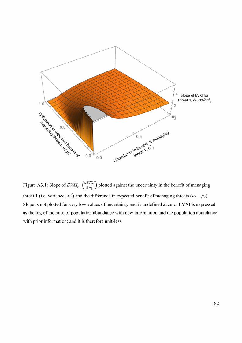
182

Figure A3.1: Slope of EVXIβ1 Mæø¿¡

M¨P™ plotted against the uncertainty in the benefit of managing

threat 1 (i.e. variance, σ12) and the difference in expected benefit of managing threats (µ1 – µ2).

Slope is not plotted for very low values of uncertainty and is undefined at zero. EVXI is expressed

as the log of the ratio of population abundance with new information and the population abundance

with prior information; and it is therefore unit-less.

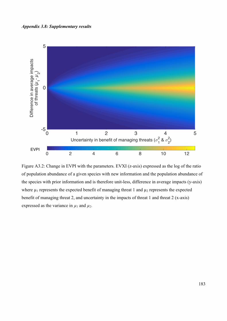
183


Figure A3.2: Change in EVPI with the parameters. EVXI (z-axis) expressed as the log of the ratio

of population abundance of a given species with new information and the population abundance of

the species with prior information and is therefore unit-less, difference in average impacts (y-axis)

where µ1 represents the expected benefit of managing threat 1 and µ2 represents the expected

benefit of managing threat 2, and uncertainty in the impacts of threat 1 and threat 2 (x-axis)

expressed as the variance in µ1 and µ2.

0 1 2 3 4 5Uncertainty in benefit of managing threats (<1

2 & <22)

-5

0

5

Diff

eren

ce in

ave

rage

impa

cts

of th

reat

s (µ

1- µ2)

0 2 4 6 8 10 12EVPI

184

Figure A3.3: Magnified cross sections of figure 4.2 showing selected strategies at fixed values for:

(a), (b), (c) difference in expected benefit of managing threats (w); (d), (e), (f) uncertainty in benefit

of managing threat 2 (σ22); and (g), (h), (i) uncertainty in benefit of managing threat 1 (σ1

2). Plots

185

generated for fixed budget (B=10). In the above figure, ‘monitor threat’ implies monitor the effect

of management on the threat.

Figure A3.4: Comparing parameter values for single species, pairs of species and all three species

used in EVXI calculations (Figure 4.4) for the case study. Plot (a) shows the expected benefit of

managing foxes (yellow) and fire (purple); and (b) shows the uncertainty in benefit of managing

foxes (yellow) and fire (purple). Species identities indicated on the x-axis. EVXI (y-axis ) is

expressed as the log of the ratio of population abundance with new information and the population

abundance with prior information; and is therefore unit-less. In case of multiple species, we

consider the expected geometric mean population abundance.

I.obe

sulus

T.vulpe

cula

M.euge

nii

I.obe

sulus

& T.vulpe

cula

I.obe

sulus

& M.eu

genii

T.vulpe

cula

& M.eu

genii

All spe

cies

0

1

2

3

4

5

6

7

Expe

cted

ben

efit

ofm

anag

ing

thre

ats

(a)

FoxesFire

I.obe

sulus

T.vulpe

cula

M.euge

nii

I.obe

sulus

& T.vulpe

cula

I.obe

sulus

& M.eu

genii

T.vulpe

cula

& M.eu

genii

All spe

cies

0

0.5

1

1.5

2

2.5

Unc

erta

inty

in b

enef

itof

man

agem

ent

(b)

FoxesFire

186

Table A3.5: EVXI values for monitoring the effect of managing foxes and fires on one, two and

three species.

Number of species Species identities EVXI (foxes) EVXI (fire)

1 I. obesulus 2.4868 0.5332 1 T. vulpecula 2.2069 1.8462 1 M. eugenii 0 0.0847 2 I. obesulus and T. vulpecula 3.3338 2.1204 2 I. obesulus and M. eugenii 0.0012 0.1001 2 T. vulpecula and M. eugenii 0.0023 0.1258 3 I. obesulus, T. vulpecula and M. eugenii 0.0072 0.0479

187

Figure A3.5: Selected monitoring strategies for the Kimberley case study. Black markers show

point estimates for σ12 in relation to the parameter space used to define the optimal monitoring

strategy for the individual species in (a), (b) and (c); and all three species in (d). Values for

uncertainty in benefit of managing foxes (σ12) fixed case as per case study data (specified above

each plot) and budget was fixed at 10. In the above figure, w = µ1 - µ2 where µ1 represents the

expected benefit of managing foxes and µ2 represents the expected benefit of managing fire.

‘Monitor foxes’ and ‘monitor fire’ imply monitoring the effect of management on foxes and fires,

respectively.

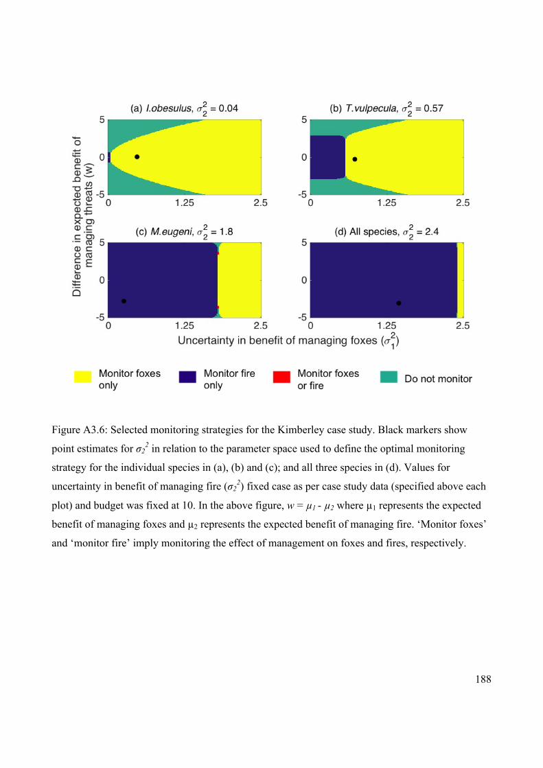
188

Figure A3.6: Selected monitoring strategies for the Kimberley case study. Black markers show

point estimates for σ22 in relation to the parameter space used to define the optimal monitoring

strategy for the individual species in (a), (b) and (c); and all three species in (d). Values for

uncertainty in benefit of managing fire (σ22) fixed case as per case study data (specified above each

plot) and budget was fixed at 10. In the above figure, w = µ1 - µ2 where µ1 represents the expected

benefit of managing foxes and µ2 represents the expected benefit of managing fire. ‘Monitor foxes’

and ‘monitor fire’ imply monitoring the effect of management on foxes and fires, respectively.

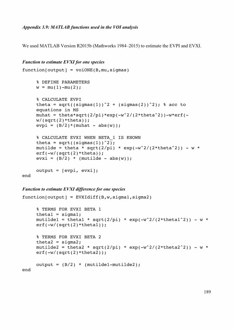
189

Appendix 3.9: MATLAB functions used in the VOI analysis

We used MATLAB Version R2015b (Mathworks 1984–2015) to estimate the EVPI and EVXI.

Function to estimate EVXI for one species

function[output] = voiONE(B,mu,sigmas)

% DEFINE PARAMETERS w = mu(1)-mu(2); % CALCULATE EVPI theta = sqrt((sigmas(1))^2 + (sigmas(2))^2); % acc to equations in MS muhat = theta*sqrt(2/pi)*exp(-w^2/(2*theta^2))-w*erf(-w/(sqrt(2)*theta)); evpi = (B/2)*(muhat - abs(w)); % CALCULATE EVXI WHEN BETA_1 IS KNOWN theta = sqrt((sigmas(1))^2); mutilde = theta * sqrt(2/pi) * exp(-w^2/(2*theta^2)) - w * erf(-w/(sqrt(2)*theta)); evxi = (B/2) * (mutilde - abs(w)); output = [evpi, evxi];

end

Function to estimate EVXI difference for one species

function[output] = EVXIdiff(B,w,sigma1,sigma2)

% TERMS FOR EVXI BETA 1 theta1 = sigma1; mutilde1 = theta1 * sqrt(2/pi) * exp(-w^2/(2*theta1^2)) - w * erf(-w/(sqrt(2)*theta1)); % TERMS FOR EVXI BETA 2 theta2 = sigma2; mutilde2 = theta2 * sqrt(2/pi) * exp(-w^2/(2*theta2^2)) - w * erf(-w/(sqrt(2)*theta2)); output = (B/2) * (mutilde1-mutilde2);

end

190


Appendix 4.1: Data sheet used for the expert elicitation for the Kimberley case study

Definition of parameters used in the data sheet: Indicators: List of potential indicators of change in threat to trigger management action Feasibility of monitoring action: Feasibility of implementing standard practice monitoring using this indicator Cost of monitoring action: Cost of implementing standard practice monitoring for this indicator (a relative measure between indicators between 0 and 100) Probability of detecting change in threat with indicator: Probability of detecting a change in threat using standard practice monitoring action for this indicator. Threats that this indicator may inform: Suggestion of change in threats informed by monitoring this indicator. In this elicitation exercise we would like you to provide your best estimate for the following columns: *** In the column ‘Cost of Monitoring - Value’ we would like you to estimate the relative costs of undertaking each indicator with the most expensive scaled to 100 and least expensive to 1. If an indicator has no cost then set it to 0. *** In the ‘Value’ columns next to each threat under ‘Probabilities of detection for a given indicator’, please provide a probability (between 0-1, where 0 is no probability of detection) of detecting the associated threat for each indicator. *** Note we have already assigned ranks in the spread sheet to help you with defining values (or to ignore). Feel free to change as you see fit.

191

Indicators

Feasibility of

monitoring action

Cost of monitoring

action (Rank)

Cost of monitoring

Value (1 to 100)

Probability of detecting change in threat with indicator

Threats that this indicator may inform on

Fire and

grazing (Rank)

Value Cat

predation (Rank)

Value Weeds (Rank) Value

Fire and

grazing

Cat predation Weeds

Stocking (exotic herbivore) density - aerial transect

highest high mod mod

Relative abundance of CWR mammals - trapping

high mod high mod

Cats sand pads high 0 mod 0 Cats remote camera high 0 mod 0

Cats trapping high 0 low 0 Cats spotlighting high 0 mod 0 Pitfall traps for small reptiles high low high low

Harp traps high low 0 0 Mist netting for birds high high mod low

Mist netting for bats high mod 0 0

Percentage perennial grass cover

low high 0 high

Percentage bare ground lowest high 0 0

Time since fire mod high 0 low

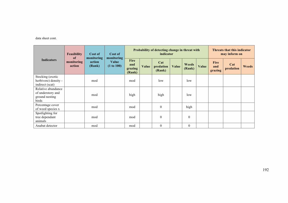
192

data sheet cont.

Indicators

Feasibility of

monitoring action

Cost of monitoring

action (Rank)

Cost of monitoring

Value (1 to 100)



Fire and

grazing (Rank)

Value Cat

predation (Rank)

Value Weeds (Rank) Value

Fire and

grazing

Cat predation Weeds

Stocking (exotic herbivore) density - indirect (scat)

mod mod low low

Relative abundance of understory and ground nesting birds

mod high high low

Percentage cover of weed species x mod mod 0 high

Spotlighting for tree dependant animals

mod mod 0 0

Anabat detector mod mod 0 0

193

Appendix 4.2: Case study data

Table A4.1: Indicators used for the Kimberly case study

ID Indicators

1 Stocking (exotic herbivore) density - aerial transect

2 Relative abundance of CWR mammals - trapping

3 Cats sand pads

4 Cats remote camera

5 Cats trapping

6 Cats spotlighting

7 Pitfall traps for small reptiles

8 Harp traps

9 Mist netting for birds

10 Mist netting for bats

11 Percentage perennial grass cover

12 Percentage bare ground

13 Time since fire

14 Stocking (exotic herbivore) density - indirect (scat)

15 Relative abundance of understory and ground nesting birds

16 Percentage cover of weed species x

17 Spotlighting for tree dependant animals

18 Anabat detector

194

Table A4.2: Species groups considered along with example species

Species group Examples

Savanna (non-rugged)

Hollow/tree structure dependant animals Non-volant (Phascogale, tree rat, rabbit rat, golden backed tree rat, black footed tree rat)

Hollow/tree structure dependant animals Volant (Yellow bellied sheath-tailed bats, cockatoos, owls) Rock-dwelling rock ringtail, rock-wallabies, rock pigeons Ground (surface and burrowing) dwelling animals

CWR mammals (Quoll, bandicoot (golden, brindled), rodents (pale field rats, western chestnut mice)

Ground (surface and burrowing) dwelling animals

Other groups (diurnal skinks, partridge pigeon, quail, thick-knees, cisticola)

Litter dwelling animals Lizards (specialist skinks, geckos)

Graminivorous animals Finches (Gouldian finch), Pigeons, small rodents (pseudomys leggadina)

Insectivorous animals Small dasyrurids, thick heads, cisticola, ibis, fairy wrens Frugivorous animals Emus, bowerbirds Nectorivores Honeyeaters and lorikeets Herbivores Macropods Predators (in response to less prey) Mulga snakes, owls, dingoes, varanids, quolls

Savanna (rugged)

Hollow/tree structure dependant animals Non-volant (Phascogale, tree rat, rabbit rat, golden backed tree rat, black footed tree rat)

Hollow/tree structure dependant animals Volant (Yellow bellied sheath-tailed bats, cockatoos, owls) Rock-dwelling rock ringtail, rock-wallabies, rock pigeons Ground (surface and burrowing) dwelling animals

CWR mammals (Quoll, bandicoot (golden, brindled), rodents (pale field rats, western chestnut mice)

Ground (surface and burrowing) dwelling animals

Other groups (diurnal skinks, partridge pigeon, quail, thick-knees, cisticola)

195

Table cont.

Species group Examples

Savanna (rugged)

Litter dwelling animals Lizards (specialist skinks, geckos) Graminivorous animals Finches (Gouldian finch), Pigeons, Rodents (pseudomys leggadina) Insectivorous animals Small dasyrurids, thick heads, cisticola, ibis, fairy wrens Frugivorous animals Emus, bowerbirds Nectorivores Honeyeaters and lorikeets Herbivores Macropods Predators (in response to less prey) Mulga snakes, owls, dingoes, varanids, quolls

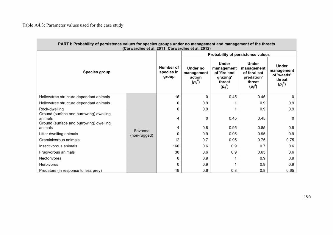
196

Table A4.3: Parameter values used for the case study

PART I: Probability of persistence values for species groups under no management and management of the threats (Carwardine et al. 2011; Carwardine et al. 2012)

Species group Number of species in

group

Probability of persistence values

Under no management

action (plj0)

Under management

of 'fire and grazing' threat (pljk)

Under management

of feral cat predation'

threat (pljk)

Under management

of 'weeds' threat (pljk)

Hollow/tree structure dependant animals

Savanna (non-rugged)

16 0 0.45 0.45 0 Hollow/tree structure dependant animals 0 0.9 1 0.9 0.9 Rock-dwelling 0 0.9 1 0.9 0.9 Ground (surface and burrowing) dwelling animals 4 0 0.45 0.45 0 Ground (surface and burrowing) dwelling animals 4 0.8 0.95 0.85 0.8 Litter dwelling animals 0 0.9 0.95 0.95 0.9 Graminivorous animals 12 0.7 0.95 0.75 0.75 Insectivorous animals 160 0.6 0.9 0.7 0.6 Frugivorous animals 30 0.6 0.9 0.65 0.6 Nectorivores 0 0.9 1 0.9 0.9 Herbivores 0 0.9 1 0.9 0.9 Predators (in response to less prey) 19 0.6 0.8 0.8 0.65

197

(Part I cont.)

Hollow/tree structure dependant animals

Savanna (rugged)

1 0.2 0.7 0.6 0.2 Hollow/tree structure dependant animals 1 0.95 1 0.95 0.95 Rock-dwelling 0 0.9 0.95 0.95 0.9 Ground (surface and burrowing) dwelling animals 0 0.2 0.7 0.6 0.2 Ground (surface and burrowing) dwelling animals 9 0.8 0.9 0.9 0.8 Litter dwelling animals 0 0.9 0.95 0.95 0.9 Graminivorous animals 0 0.9 0.95 0.95 0.9 Insectivorous animals 28 0.8 0.9 0.85 0.8 Frugivorous animals 3 0.8 0.95 0.85 0.8 Nectorivores 0 0.95 1 0.95 0.95 Herbivores 4 0.95 1 0.95 0.95 Predators (in response to less prey) 41 0.5 0.7 0.8 0.5

PART II: Parameter values for threats and management actions specific to the threats (Carwardine et al. 2011; Carwardine et al. 2012)

Threats What is prior belief in the

impact of this threat? (bj)

What is best action for threat?

E.g. From your prioritisation the most cost effective action

for each threat

What is the Feasibility of that action?

(Fkj)

Fire and Grazing 0.67 Complex 0.75 Cat predation 0.98 Complex 0.25 Weeds 0.5 Complex 0.625

198

PART III: Parameter values for indicators (obtained through expert elicitation)

Indicators

Feasibility of

monitoring action

Cost of monitoring

Value (1 to 100)



Fire and grazing

Cat predation Weeds Fire and

grazing Cat

predation Weeds

Stocking (exotic herbivore) density - aerial transect 1 70 1 0 0 x

Relative abundance of CWR mammals - trapping 0.8 90 0.8 0.6 0 x x

Cats sand pads 0.5 80 0 0.7 0 x Cats remote camera 1 40 0 1 0 x Cats trapping 0.4 100 0.2 0.8 0 x x Cats spotlighting 0.6 70 0.1 0.7 0 x x Pitfall traps for small reptiles 0.8 80 0.8 0.6 0 x x Harp traps 0.3 60 0 0 0 Mist netting for birds 0.5 60 0 0 0 Mist netting for bats 0.3 60 0 0 0 Percentage perennial grass cover 0.9 10 1 0 0.2 x x Percentage bare ground 1 1 1 0 0 x Time since fire 1 30 1 0 0 x Stocking (exotic herbivore) density - indirect (scat) 0.8 10 0.5 0 0 x

Relative abundance of understory and ground nesting birds 0.8 50 0.7 0.5 0.1 x x x

Percentage cover of weed species x 0.8 20 0.7 0 1 x x Spotlighting for tree dependant animals 0.5 40 0 0.2 0 x Anabat detector 0.3 20 0 0 0

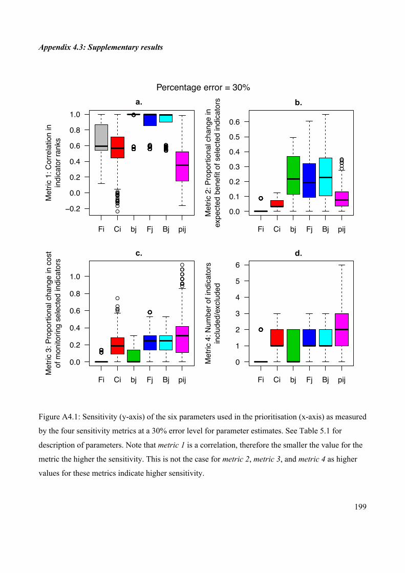
199


Figure A4.1: Sensitivity (y-axis) of the six parameters used in the prioritisation (x-axis) as measured

by the four sensitivity metrics at a 30% error level for parameter estimates. See Table 5.1 for

description of parameters. Note that metric 1 is a correlation, therefore the smaller the value for the

metric the higher the sensitivity. This is not the case for metric 2, metric 3, and metric 4 as higher

values for these metrics indicate higher sensitivity.

●

●

●

●●●

●●●

●

●

●●

●●

●●●

●

●●●●●

●

●●

●

●●●

●

●●●●

●●

●

●●

●●●●

●

●●●●●●

●

●●

●

●

●

●

●

●●●

●

●●

●

●●

●

●●●●●●

●

●●●●

●

●●●

●

●●●●

●

●●●●

●

●●

●

●●●●●●●●●●●●●●●

●

●

●

●●●●

●●●

●

●

●●

●

●●●●●

●

●●●●

●

●●●●●●●●●●

●

●

●

●●●●●●

●

●●●●●

●

●●●●●●●● ●

●●●●●●●●●●●●●●●●●●●●●●●●●●●●●●●●●●●●●●●●●●●●●●●●●●●●●●●●●●●●●●●●●●●●●●●●●●●●●●●●●●●●●●●●●●●●●●●●●●●●●●●●●●●●●●●●●●●●●●●●●●●●●●●●●●●●●●●●●●●●●●●●●●●●●●●●●●●●●●●●●●●●●●●●●●●●●●●●●●●●●●●●●●●●●●●●●●●●●●●●●●●●●●●●●●●●●●●●●●●●●●●●●●●●●●●●● ●

●●●●●●●●●●●●●●●●●●●●●●●●●●●●●●●●●●●●●●●●●●●●●●●●●●●●●●●●●●●●●●●●●●●●●●●●●●●●●●●●●●●●●●●●●●●●●●●●●●●●●●●●●●●●●●●●●●●●●●●●●●●●●●●●●●●●●●●●●●●●●●●●●●●●●●●●●●●●●●●●●●●●●●●●●●●●●●●●●●●●●●●●●●●●●●●●●●●●●●●●●●●●●●●●●●●●●●●●●●●●●●●●●●●●●●●●●●●●●●●●

Fi Ci bj Fj Bj pij

−0.2

0.0

0.2

0.4

0.6

0.8

1.0

Met

ric 1

: Cor

rela

tion

inin

dica

tor r

anks

●●●●●●●●●●●●●●●●●●●●●●●●●●●●●●●●●●●●●●●●●●●●●●●●●●●●●●●●●●●●●●●●●●●●●●●●●●●●●●●●●●●●●●●●●●●●●●●●●●●●●●●●●●●●●●●●●●●●●●●●●●●●●●●●●●●●●●●●●●●●●●●●●●●●●●●●●●●●●●●●●

●

●

●●

●●●

Fi Ci bj Fj Bj pij

0.0

0.1

0.2

0.3

0.4

0.5

0.6

Met

ric 2

: Pro

porti

onal

cha

nge

inex

pect

ed b

enef

it of

sel

ecte

d in

dica

tors

●●●●●●●●●●●●●●●●●●●●●●●●●●●●●●●●●●●●●●●●●●●●●●●●●●●●●●●●●●●●●●●●●●●●●●●●●●●●●●●●●●●●●●●●●●●●●●●●●●●●●●●●●●●●●●●●●●●●●●●●●●●●●●●●●●●●●●●●●●●●●●●●●●●●●●●●●●

●●●

●

●

●●●●●●●●●●●●●●●●●●●●●●●●●●●●●●●●●●●●●●●●●●●●●●●●●●●●●●●●●●●●●●●

●●●●

●

●●●

●●●●

●

●●●

●●

●

●●

●

●●●●●

Fi Ci bj Fj Bj pij

0.0

0.2

0.4

0.6

0.8

1.0

Met

ric 3

: Pro

porti

onal

cha

nge

in c

ost

of m

onito

ring

sele

cted

indi

cato

rs

●●●●●●●●●●●●●●●●●●●●●●●●●●●●●●●●●●●●●●●●●●●●●●●●●●●●●●●●●●●●●●●●●●●●●●●●●●●●●●●●●●●●●●●●●●●●●●●●●●●●●●●●●●●●●●●●●●●●●●●●●●●●●●●●●●●●●●●●●●●●●●●●●●●●●●●●●●●●●●●●●●●●●●●●●●●●●

Fi Ci bj Fj Bj pij

0

1

2

3

4

5

6

Met

ric 4

: Num

ber o

f ind

icat

ors

incl

uded

/exc

lude

d

Percentage error = 30%a. b.

c. d.

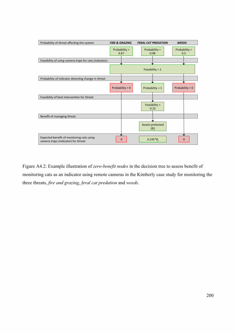
200

Figure A4.2: Example illustration of zero-benefit nodes in the decision tree to assess benefit of

monitoring cats as an indicator using remote cameras in the Kimberly case study for monitoring the

three threats, fire and grazing, feral cat predation and weeds.

Feasibility*=*1*

Probability*of*threat&affec3ng*the*system: ******** ******FIRE%&%GRAZING%%%%%%%%FERAL%CAT%PREDATION %%%%%%%%WEEDS&

Feasibility*of*using&camera&traps&for*cats&(indicator):*

Probability*of*indicator*detec3ng*change*in*threat:*

Feasibility*of*best*interven3on*for*threat:*

Benefit*of*managing*threat:&

Expected*benefit*of*monitoring*cats&using&camera&traps&(indicator)*for*threat:*

Probability*=*1*

Feasibility*=*0.25*

Assets*protected*(Bj)*

0.245*Bj&&

Probability*=*0.98*

Probability*=*0*

0*

Probability*=*0.5*

Probability*=*0*

0*

Probability*=*0.67*

effective monitoring for biodiversity conservation562951/s4300559_final_thesis.pdf · eve...

Documents