effective coupling of signal timing estimation model and ...docs.trb.org/prp/14-4957.pdf · 1...

Effective Coupling of Signal Timing Estimation Model and Dynamic Traffic Assignment in 1

Feedback Loops: System Design and Case study 2

3

4

5

6

7

8

Milan Zlatkovic 9 Research Assistant Professor 10

Department of Civil and Environmental Engineering 11

University of Utah 12

110 Central Campus Dr., Rm. 2000B 13

Salt Lake City, Utah 84112 14

Phone: (801) 819-5925 15

Fax: (801) 585-5860 16

E-mail: [email protected] 17

18

19

20

Xuesong Zhou* 21 Associate Professor 22

School of Sustainable Engineering and the Built Environment 23

Arizona State University 24

Tempe, AZ 85287, USA 25

Email: [email protected] 26

27

*Corresponding Author 28

29

30

31

32

33

34

35

36

37

38

Word Count: 5739 + 1750 (5 Figures + 2 Tables) = 7489 39

40

41

Submitted for publication and presentation considerations at the 93rd meeting of the 42

Transportation Research Board 2014 43

44

45

TRB 2014 Annual Meeting Original paper submittal - not revised by author

Zlatkovic, M., and Zhou, X. 2

ABSTRACT 1

This paper presents an integrated framework for effective coupling of a signal timing estimation 2

model and Dynamic Traffic Assignment (DTA) in feedback loops. There are many challenges in 3

effectively integrating signal timing tools with DTA software systems, such as data availability, 4

exchange format, and system coupling. In this research, a tight coupling between a DTA model 5

with various queue-based simulation models, and a Quick Estimation Method (QEM) Excel-6

based signal control tool is achieved and tested. The presented framework design offers an 7

automated solution for providing realistic signal timing parameters and intersection movement 8

capacity allocation, especially for future year scenarios. The framework was used to design an 9

open-source data-hub for multi-resolution modeling in Analysis, Modeling and Simulation 10

(AMS) applications, in which a typical regional planning model can be quickly converted to 11

microscopic traffic simulation and signal optimization models. The coupling design and 12

feedback loops are first demonstrated on a simple network, and we examine the theoretically 13

important questions on the number of iterations required for reaching stable solutions in 14

feedback loops. As shown in our experiment, the current coupled application becomes stable 15

after about 30 iterations, when the capacity and signal timing parameters can quickly converge, 16

while DTA’s route switching model predominately determines and typically requires more 17

iterations to reach a stable condition. A real-world work zone case study illustrates how this 18

application can successfully be used to assess impacts of road construction or traffic incident 19

events that disrupt normal traffic operations and cause route switching on multiple analysis 20

levels. 21

22



1. INTRODUCTION 1

Dynamic traffic assignment (DTA) models have been increasingly recognized as an important 2

tool for assessing operational performances at different spatial, and across various analysis 3

temporal regimes. The advances of DTA in this aspect are built upon the capabilities of DTA 4

models in describing the formation, propagation and dissipation of traffic congestion in a 5

transportation network. Planning practitioners have recognized the full potential of DTA 6

modeling methodologies that describe within-day and day-to-day network-level and corridor-7

level congestion in a transportation network with Advanced Traffic Management and Advanced 8

Traveler Information provision strategies (1). 9

The coupling of traffic assignment and signal control has long been a focus of numerous 10

research efforts. However, due to the complexity of the problem, usually one of two approaches 11

is used: (a) assuming fixed signal control (capacities) and using DTA to perform network 12

loading; (b) assuming fixed traffic assignment and performing signal control evaluation and 13

optimization (2, 3). Model coupling can be achieved on multiple levels, such as full integration, 14

close coupling, loose coupling and isolated approach (4, 5). 15

While leading-edge research is underway that will significantly advance transportation 16

modeling practices, current signal timing estimation tools (e.g. Synchro, TRANSYT-7F, 17

PASSER) have not been designed to facilitate integrated modeling and practices in combining 18

signal timing and DTA, so these processes are largely ad-hoc and relatively inefficient. Many 19

planners have found numerous challenges in effectively integrating signal timing tools with DTA 20

software systems, such as data availability, exchange format, and system coupling. Determining 21

accurate signal timing data requires precise inputs on intersection geometry and turning volumes. 22

The types of data required for inputs into models are not available, or are difficult to obtain from 23

existing regional planning data, which typically only have the number of through lanes as link 24

level attributes. External data sources, particularly movement-specific attributes, can be coded in 25

signal timing package’s format, such as Synchro’s Uniform Traffic Data Format (UTDF). 26

Although these data are becoming increasingly available for use in transportation planning 27

applications, the data sources are not yet easily integrated into standard regional planning 28

practices and still require significant labor resources to map signal locations, and convert the data 29

to a useful format for existing DTA packages. 30

In the current planning practice, the lack of standardized signal data formats calls for 31

manual manipulation or customization of utility tools to interface between planning models and 32

signal timing estimation models. One solution to this challenge is to develop an open data format 33

that allows software vendors and planners to implement data conversion utilities from their own 34

proprietary format. For maximum effectiveness, this research develops open data format through 35

a publicly visible, vendor-independent process to ensure interoperability among diverse traffic 36

modeling and simulation tools. 37

Although a full integration approach that builds both signal timing estimation and DTA 38

on same design is desirable for multi-resolution modeling, this approach makes the extensions of 39

individual models very difficult. Therefore, a tight coupling approach that can use well defined 40

data format to transfer data files between different resolutions of common models is more 41

desirable in order to achieve scalability, modularity, interoperability, and extendibility. Along 42

this line, the individual models can be developed on the modular basis, where each module can 43

perform its function and can be easily connected and extended to meet future modeling needs. 44

One of the most significant gaps in the functionality of current multi-resolution modeling 45

systems is the lack of behavioral response associated with (1) capacity allocation at signalized 46



intersections, (2) traffic congestion due to route diversion and (3) other demand management 1

strategies such as road pricing. Transportation models in many cases require significant 2

manipulation and calibration to produce reasonable results for networks that are over saturated 3

and/or include demand management strategies that affect travelers’ choice of mode, departure 4

time, and route. However, by only focusing on the “demand” side of congestion modeling, many 5

transportation analyses do not reflect the true effects of operating conditions, particularly when it 6

comes to examining signalized intersection performance over multiple days for the purposes of 7

estimating reliability. Therefore many practitioners have observed a critical need for a seamless 8

feedback loop between DTA and signalized intersections capacity allocation. 9

The demonstration prototype of this study aims to integrate an open-source DTA system, 10

called DTALite, with an Excel-based signal timing estimation tool, called the Quick Estimation 11

Method (QEM). Specifically, a tight coupling between the two models has been developed, 12

enabling a simultaneous assessment of traffic assignment and traffic signals, through an open-13

source Analysis, Modeling and Simulation (AMS) data-hub, namely Network Explorer for 14

Traffic Analysis (NEXTA) GUI. The integration of the two models and the feedback loop 15

procedure are described on a simple two-route network, and their full capabilities are 16

systematically tested on a real-world network with a work zone application example. The 17

developed QEM tool can be also easily coupled with other DTA packages, such as 18

DYNASMART and TRANSIMS, as AMS data hub can serve as a data exchange utility for a 19

number of simulation packages. 20

Majority of research in the combined traffic assignment-traffic control environment has 21

been performed for either DTA and fixed signal control, or static assignment and signal control 22

optimization. One mathematical formulation that uses incremental assignment logic is presented 23

in (6) and (7). This is basically an extension of signal optimization under the static assignment, 24

where the signals were repeatedly adjusted for small added portions of the demand until the total 25

demand was loaded. Another conceptual solution framework consisting of two interactive loops 26

for the combined optimization problem is described in (8). However, very limited real-world 27

implementation or numerical application with widely used signal timing standard (e.g. HCM 28

methodology) was performed within the proposed framework. A mathematical formulation and 29

heuristic simulation-based procedure to obtain time-varying assignment of OD vehicles to paths 30

jointly with time-varying signal settings that seek to optimize the total travel time in the network 31

is given in (2). This framework was tested on the Dallas-Fort Worth network with three 32

congestion levels. The implementation of the designed algorithm decreased average travel times 33

in the network, and showed promising results related to the convergence. Another integrated 34

framework that uses the game theory to model the combined DTA-traffic signal problem is 35

explored in (9). In their research, the dynamic traffic control problem and DTA are integrated as 36

a non-cooperative game between a traffic authority and highway users. 37

Bi-level programming and optimization has been widely used to examine the combined 38

DTA-traffic control problem. Sun et al. (3) developed a bi-level programming formulation and 39

heuristic solution approach for dynamic traffic signal optimization in networks with time-40

dependent demand and stochastic route choice. In their solution approach, Genetic Algorithm is 41

used to find the upper level signal control variables, Incremental Logit Assignment is developed 42

to find the user optimal flow pattern in the lower level problem, and Cell Transmission 43

Simulation is implemented to propagate traffic and collect real-time traffic information. The 44

study showed that the heuristic solution approach can provide a realistic representation of traffic 45

operation in both network and link level operational performance. Another bi-level formulation 46

for the combined dynamic equilibrium and signal control, presented in (10), defines a signal 47



control operator in the upper level that optimizes the signal setting to minimize the system travel 1

time, while the road users in the lower level minimize their own costs, leading to dynamic user 2

equilibrium. The projection algorithm was used to solve the lower level, and the mixed integer 3

programming solver to solve the upper level. The algorithm was successfully tested on 4

hypothetical networks with one and multiple signalized intersections. 5

Focusing on effective software system integration for transportation planning 6

applications, our paper presents a data exchange and software coupling framework in which two 7

models, DTALite (as a representative mesoscopic DTA package) and QEM signal timing 8

estimation, are successfully linked to address practical needs for providing realistic signal timing 9

parameters and intersection movement capacity allocation, especially for future year scenarios. 10

The next section provides descriptions of the general DTA assignment-simulation model and 11

computational engine. The QEM signal timing methodology and application are described in 12

section 3. Section 4 describes the coupling of the two models and demonstrates the feedback 13

loop and their convergence on a simple two-route network. The framework is tested on a real-14

world network with a work zone implementation in section 5. 15

16

2. MODELING COMPONENTS OF MESOCOPIC DTA PACKAGES 17

As a newly developed open source DTA package, DTALite uses a number of computationally 18

simple but theoretically rigorous traffic queuing models in its lightweight mesoscopic simulation 19

engine. Similar to many existing mesoscopic DTA packages, the four major modeling 20

components in the DTALite system architecture are summarized as follows: (i) Time-dependent 21

shortest path finding based on a node-link network structure from regional planning models; (ii) 22

vehicle/agent attribute generation that converts OD demand matrices in conjunction with 23

additional time-of-day departure time profile, as well as possible variable value of time 24

distribution. (iii) DTA method that considers major factors affecting agents’ route choice, such 25

as different types of traveler information and road pricing strategies, and (iv) a wide range of 26

traffic flow models, namely point queue, spatial queue with jam density constraint and simplified 27

kinematic wave models, are available to model essential road capacity reduction or enhancement 28

measures. 29

The traffic assignment and simulation modules are integrated and iterated to either 30

capture day-to-day user response, or find steady-state equilibrium conditions. Within this 31

simulation-assignment framework, the rich set of output data include traffic MOEs at different 32

spatial and temporal scales, ranging from network, corridor-level, links and movements. Typical 33

speed, volume and density measures and agent-based trajectories can be visualized and 34

processed through the NeXTA user interface. Overall, DTALite uses a link-based and 35

movement-based simulation architecture with capacity constraints at both link and movement 36

levels. The capacity constraints make calibrating network capacities a very important step in the 37

process of building our models. On the other hand, the open-source code base, accessible at 38

https://code.google.com/p/nexta/, can be flexibly used to enhance to meet specific modeling 39

needs. 40

41

3. QEM METHODOLOGY AND EXCEL-BASED APPLICATION 42

By adapting the methodology from Highway Capacity Manual (HCM) 2010 (11), QEM is a 43

simplified method for determining the signal timing parameters, critical intersection volume-to-44

capacity (V/C) ratio, and delay for a signalized intersection. To reduce the data input efforts for 45



DTA and other planning applications, this methodology requires only minimal intersection 1

geometry and traffic data, such as the approach lane configuration and turning volumes. It 2

assumes certain default values for some of the variables which are integrated into the calculation 3

methodology. QEM provides approximate intersection performance results for the known signal 4

timing parameters, or calculates the signal timing using a simplified calculation procedure based 5

on the critical movement methodology. 6

The QEM Excel-based calculation engine can perform signal timing calculation and 7

capacity assessment of signalized intersections based on the user-defined inputs, or inputs passed 8

to it through AMS applications. The QEM Excel tool also uses some additional signal timing 9

calculation, given in the Signal Timing Manual (12) and Utah Department of Transportation 10

(UDOT) standards (13). It can work as a stand-alone application, or integrated with NeXTA. The 11

QEM software package can be downloaded at 12

https://drive.google.com/?tab=wo&authuser=0#folders/0Bw8gtHCvOm7WTjg0a2FvdlhrRjQ. 13

The QEM calculation steps are given in Figure 1. 14

15

16

FIGURE 1 QEM calculation steps. 17 18

Based on the given inputs, this step first determines the intersection major and minor 19

approaches, and then sets the initial phase numbers to through and left turns Once the initial 20

phasing is selected, the spreadsheet determines the left turn treatment as protected only, 21

protected plus permitted, or permitted only for each intersection approach. After the left turn 22

Geometry, volume and

calculation inputs

Phase designation

Left turn treatment

Dual ring-barrier structure

Lane group volumes

Signal timing parameters:

cycle, green times, capacity,

V/C, delay, LOS, status

Outputs:

Visualization,

NeXTA GUI

Inputs

Step 1

Step 2

Step 3

Outputs



treatment is selected, the dual ring-barrier phase structure is defined, with all phases which are 1

used in the given case. 2

The second step uses the given intersection geometry and traffic inputs, and applies the 3

HCM methodology to compute lane volumes for each lane group. This procedure takes into 4

consideration the number of lanes for each approach, lane assignment, right-turn-on–red 5

volumes, and left turn treatment. These volumes are then used in the follow-up calculations. 6

Once the phasing plan, left turn treatment and lane volumes are known, signal timing 7

parameters can be computed in the third step as follows: 8

a) Compute saturation flow rates for protected, permitted and protected plus permitted 9

movements 10

b) Compute critical phase volume and lost time 11

c) Compute critical sum and cycle lost time 12

d) Determine cycle length 13

e) Compute phase green times and splits 14

15

The critical phase volume (CV) is the volume for the movement that requires the longest 16

green time during the phase. A phase plan summary table, which includes movement codes and 17

sequences from previous steps, is used to determine the phase plan summary and identify the 18

critical sequence of movements within the signal cycle. This table also determines the lost time l 19

assigned to each phase. When all phases have been completed, the critical sum (CS) of the 20

critical phase volumes is computed. The cycle lost time L represents the sum of the phase lost 21

time for each of the critical phases. 22

Once the critical phases have been determined and CV, CS and L computed, the cycle 23

length is calculated as: 24

25

(1)

26

Where: 27

28

C – Cycle length (s) 29

Cmin – Minimum cycle length (s) 30

Cmax – Maximum cycle length (s) 31

L – Sum of cycle lost time (s) 32

CS – Critical sum (veh/h) 33

RS – Reference sum flow rate (veh/h), 34

PHF – Peak Hour Factor 35

fa – Area type adjustment factor (0.9 for Central Business District – CBD, 1.0 36

otherwise) 37

38

When the cycle length is determined, the spreadsheet calculates phase split (inter-green) 39

times g for the phases determined in the ring-barrier structure. These times are determined by the 40

following equation: 41

42

(2)



1

where g is the phase split time (s), CV is the critical phase flow rate (veh/h), and gmin is the 2

minimum split time, which is set to nine seconds in the algorithm. 3

Furthermore, the spreadsheet calculates additional phasing data, such as the effective 4

phase green times and capacities based on the HCM methodology, and yellow, red clearance, 5

pedestrian walk and flash-don’t-walk times, based on the methodology described in (12) for the 6

given intersection geometry and traffic characteristics. When all the data are known, the 7

spreadsheet produces the intersection MOEs, which include capacities and V/C ratios for all 8

movements, as well as the critical intersection V/C, control delay per vehicle, intersection LOS 9

and intersection status. 10

As an important level of service measure, the control delay in the spreadsheet is 11

calculated as the sum of the uniform delay, which is the delay that occurs if arrival demand in the 12

lane group is uniformly distributed over time, and the incremental delay, which accounts for 13

some randomness in vehicle arrivals. The uniform and incremental delays for each lane group 14

are calculated as follows: 15

16

(3)

(4)

(5)

where X is the lane group V/C ratio, c is the lane group capacity (veh/h), T is the duration of the 17

analysis period (h), and other variables as previously defined. The critical intersection V/C ratio 18

XC is calculated as follows: 19

20

(6)

21

The calculated intersection parameters and MOEs are communicated back to the user, 22

and the interface depends whether the QEM spreadsheet is used as a stand-alone application, or 23

integrated with NeXTA. If used as a stand-alone application, the user can view the results in a 24

specially designed Summary Sheet, or can export them as a PDF report. In NeXTA, the user can 25

select and view the intersection results in the node editor. 26

27

4. COUPLING QEM AND DTA SOFTWARE PACKAGES 28

Figure 2 shows the model coupling, information flow and feedback loop between simulation and 29

signal timing estimation modules. 30



1 2

FIGURE 2 DTALite and QEM coupling and feedback loop. 3 4

In order to fully integrate multiple stand-alone models or simulation programs, it is 5

important to standardize data exchange between those tools at different levels of resolution. In 6

addition, open standard will enhance the interoperability of simulations (or applications or 7

systems) to coordinate and work together in a common (virtual) environment. This ability 8

requires the AMS architecture to be built on a common understanding of data schema for traffic 9

modeling and simulation, in particular, transportation network, traffic demand, traffic control 10

devices as well as traffic sensor data. The data formats typically used in the system coupling 11

consist of customized binary files, comma-separated values (CSV), Extensible Markup Language 12

(XML), and database formats. In this research, we use CSV format, which allows a successful 13

and rapid integration with other modeling tools, creating a feasible environment for cross-14

resolution modeling applications. In Table 1, we provide a summary of different model coupling 15

approaches that can be used to integrate two software systems. In our software prototype, the 16

tight system coupling between the two models is implemented through Excel-based data 17

exchange interfaces, such as Excel Automation. Based on a subset of Component Object 18

Model (COM), Excel Automation is an inter-process communication mechanism created 19

by Microsoft. It has been supported by many programming languages such as C++ and Java. 20

21

Network

geometryNeXTA

OD Demand

matrixDTALite

Node/Link/Zone

Demand type/Vehicle type

Path flow

AMS

Movement fileQEM

Movement

volumes

Simulation

outputs

Movement

capacities

Feedback loop

Output

Visualization

Excel

Automation

Dual ring

phasing



TABLE 1 Simulation/Model Coupling Approach Comparison Summary 1 2

Approach Key features Advantages Disadvantages

External Executables/

Stand-Alone programs

Use text file as input and

output between programs

Configuration file or batch

file to control iteration flow

Call perform manual

iterations using difficult

programs

No change to existing

programs

Easy programming calling

on the same machine

Easy to be debugged by

planners/models

Ad-hoc one-to-one

program interface

Extensive file exchanges

Loose coupling between

programs

Static or dynamic

programming library

API, Lib, dynamic

linking library (DLL),

OCX, Active X, COM

Users provide simulation-

callable DLL

Simulation programs will

embed the user-defined

library during the execution

of application

Unified programming

interface

Efficient integration for

specific functionalities such

as signal timing control or

vehicle statistic calculation

(trigged by vehicle

movement functions)

Relatively limited

functionalities

Require familiarity of

advanced programming

languages (e.g. C or C++)

Only supports data

exchange on the local

machine

Message passing and

inter-program data

sharing

Common Object

Request Broker

Architecture (CORBA)

Use Interface Definition

Language (IDL) to specify

a mechanism in software

for standardizing the

method-call semantics

between application objects

Written in multiple

programming languages,

integrate large-scale

simulation programs

running on multiple

computers/different

platforms

Extremely complex

programming interface

Web service in cloud

computing

Service provider pool the

processing power of

multiple remote computers

in a cloud to perform

simulation/modeling tasks

Allow integrated data

collection, data sharing

and traffic modeling

Perform simulation tasks

might normally be difficult,

time consuming, or

expensive for an individual

user or a small company to

accomplish, especially with

limited computing

resources and funds

Only suitable to routine

tasks with extensive user

debugging,

Difficult for modelers to

debug and examine

simulation results

3

4



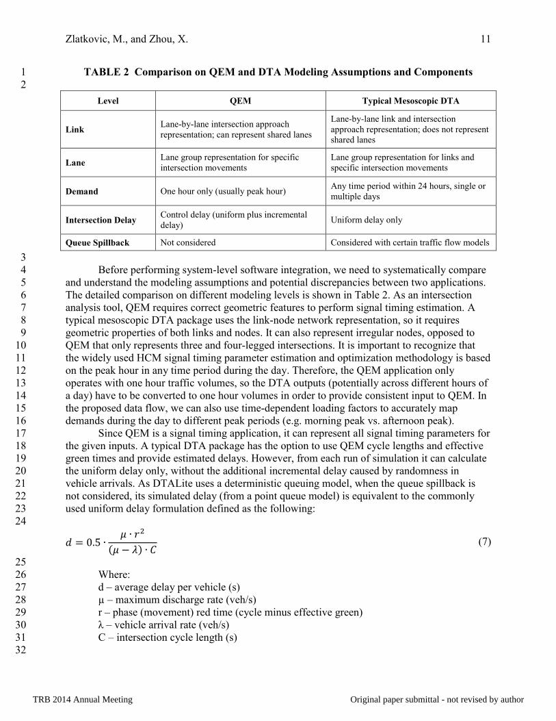
TABLE 2 Comparison on QEM and DTA Modeling Assumptions and Components 1

2

Level QEM Typical Mesoscopic DTA

Link Lane-by-lane intersection approach

representation; can represent shared lanes

Lane-by-lane link and intersection

approach representation; does not represent

shared lanes

Lane Lane group representation for specific

intersection movements

Lane group representation for links and

specific intersection movements

Demand One hour only (usually peak hour) Any time period within 24 hours, single or

multiple days

Intersection Delay Control delay (uniform plus incremental

delay) Uniform delay only

Queue Spillback Not considered Considered with certain traffic flow models

3

Before performing system-level software integration, we need to systematically compare 4

and understand the modeling assumptions and potential discrepancies between two applications. 5

The detailed comparison on different modeling levels is shown in Table 2. As an intersection 6

analysis tool, QEM requires correct geometric features to perform signal timing estimation. A 7

typical mesoscopic DTA package uses the link-node network representation, so it requires 8

geometric properties of both links and nodes. It can also represent irregular nodes, opposed to 9

QEM that only represents three and four-legged intersections. It is important to recognize that 10

the widely used HCM signal timing parameter estimation and optimization methodology is based 11

on the peak hour in any time period during the day. Therefore, the QEM application only 12

operates with one hour traffic volumes, so the DTA outputs (potentially across different hours of 13

a day) have to be converted to one hour volumes in order to provide consistent input to QEM. In 14

the proposed data flow, we can also use time-dependent loading factors to accurately map 15

demands during the day to different peak periods (e.g. morning peak vs. afternoon peak). 16

Since QEM is a signal timing application, it can represent all signal timing parameters for 17

the given inputs. A typical DTA package has the option to use QEM cycle lengths and effective 18

green times and provide estimated delays. However, from each run of simulation it can calculate 19

the uniform delay only, without the additional incremental delay caused by randomness in 20

vehicle arrivals. As DTALite uses a deterministic queuing model, when the queue spillback is 21

not considered, its simulated delay (from a point queue model) is equivalent to the commonly 22

used uniform delay formulation defined as the following: 23

24

(7)

25

Where: 26

d – average delay per vehicle (s) 27

µ – maximum discharge rate (veh/s) 28

r – phase (movement) red time (cycle minus effective green) 29

λ – vehicle arrival rate (veh/s) 30

C – intersection cycle length (s) 31

32



In the current form, QEM does not calculate queue lengths, and therefore it is not able to 1

provide information on queue spillback and upstream intersection blockage. On arterial streets, 2

DTALite can use spatial queue models that can determine queue lengths and spillback, so it can 3

assess the impacts of lane blockage. From this comparison, it can be seen that QEM and 4

DTALite supplement each other to provide a detailed analysis on any network level. 5

6

4.1. DTA and QEM Feedback Loop Convergence 7 8

Essentially, the feedback loop in the coupled system operates as the following sequence. 9

10

1) Initial traffic flow volumes are calculated from traffic assignment package based on 11

capacity values associated with BPR functions from the regional planning model. 12

2) As a dynamic, traffic responsive system, QEM determines and changes intersection 13

movement capacities based on the current traffic volumes. 14

3) With re-estimated movement capacity or signal timing from QEM, a DTA program 15

simulates traffic flow along each path subject to the new capacity constraints at each 16

signalized intersection, and then recalculates experienced travel time along each path. 17

The route switching algorithm will use either MSA or proportional switch to adjust path 18

flow volume at different departure time intervals, which further affect link or movement 19

volumes coming through the QEM controlled intersections. Essentially, the new 20

capacities from step 2 can impact DTA and cause traffic rerouting among available 21

routes. 22

4) Increase iteration counter by 1. Check the convergence patterns in assignment travel flow 23

volumes, if the link flow changes between two iterations then go to step 2 to estimate the 24

signal timing parameters, and therefore movement capacities. 25

26

To test the feedback loop and the simultaneous convergence in the DTA-QEM framework, a 27

simple network with two between one origin and one destination is tested. The network is shown 28

in Figure 3 a), and the inputs are as follows: 29

30

Analysis period = 60 min 31

OD demand = 9000 veh/h 32

Freeway distance = arterial distance = 3 miles 33

Freeway free flow travel time = 3 min 34

Arterial free flow travel time = 4.5 min 35

Number of lanes freeway = 2 36

Number of lanes arterial = 3 37

Freeway capacity = 4000 veh/h 38

39

One signalized intersection is assumed to located in the middle of the arterial corridor. 40

The cross-traffic at the intersection is set to be 450 veh/h, with no left or right turns. For 41

simplicity, it is assumed that there is no flow in the opposite direction along the main corridor. 42

The current cycle length, main movement effective green time, capacity, V/C ratio and 43

delay are obtained through QEM for each iteration and for the current volume assigned to the 44

arterial corridor, and that movement capacity is used in the next iteration. The feedback loop of 45

assignment-signal timing adjustment is performed for 100 iterations. The convergence patterns 46

are shown in Figure 3 b) – c), where Figure 3 b) shows a comparison of travel times, Figure 3 c) 47



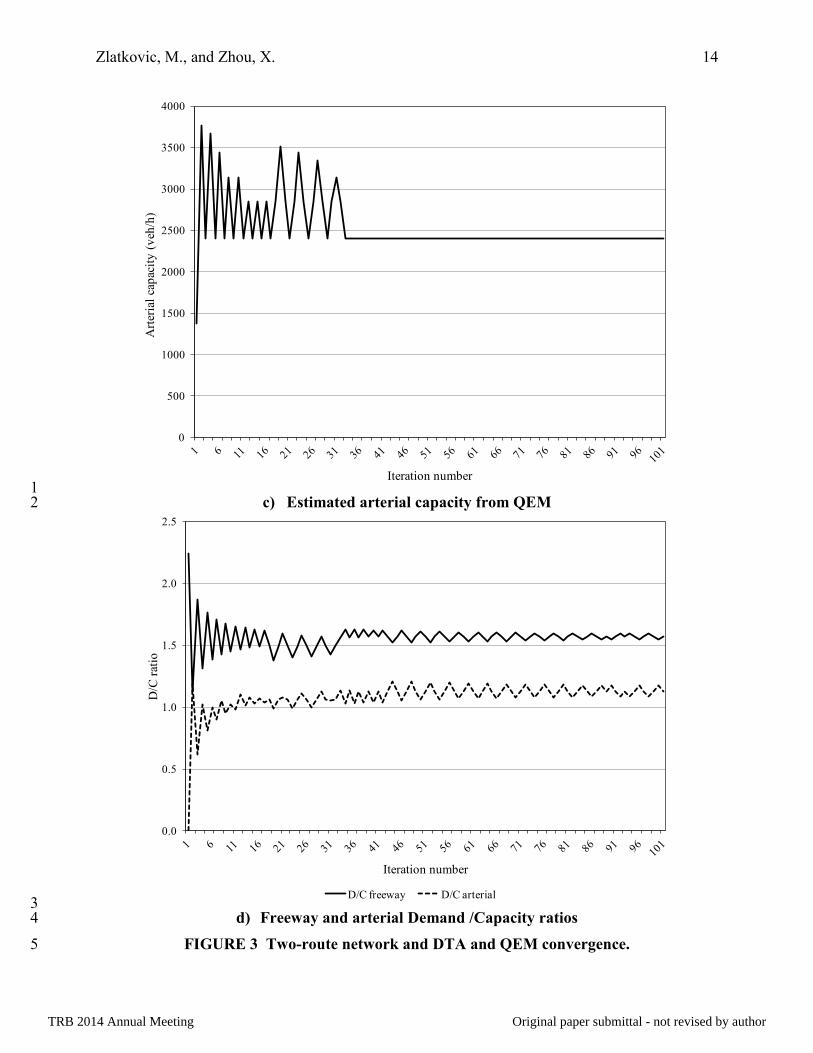
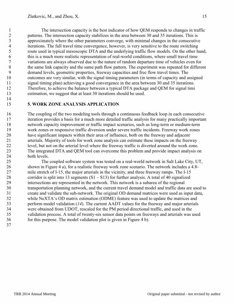
shows the movement capacity at the intersection, and Figure 3 d) shows a comparison of 1

demand-to-capacity (D/C) ratios. 2

3

4 a) Two-route network inputs 5

6

7 b) Freeway and arterial travel times from traffic assignment program 8

9

Origin Destination

Freeway

Arterial Signalized

intersection

L = 3 miles

FFTT = 3 min

L = 3 miles

FFTT = 4.5 min

OD demand = 9000 veh/h

450 veh/h

450 veh/h

0

2

4

6

8

10

12

14

16

Tra

vel

Tim

e (m

in)

Iteration number

Freeway TT Arterial TT



1 c) Estimated arterial capacity from QEM 2

3 d) Freeway and arterial Demand /Capacity ratios 4

FIGURE 3 Two-route network and DTA and QEM convergence. 5

0

500

1000

1500

2000

2500

3000

3500

4000

Art

eria

l ca

pac

ity

(v

eh/h

)

Iteration number

0.0

0.5

1.0

1.5

2.0

2.5

D/C

rat

io

Iteration number

D/C freeway D/C arterial



The intersection capacity is the best indicator of how QEM responds to changes in traffic 1

patterns. The intersection capacity stabilizes in the area between 30 and 35 iterations. This is 2

approximately where the other parameters converge, with minimal changes in the consecutive 3

iterations. The full travel time convergence, however, is very sensitive to the route switching 4

route used in typical mesoscopic DTA and the underlying traffic flow models. On the other hand, 5

this is a much more realistic representation of real-world conditions, where small travel time 6

variations are always observed due to the nature of random departure time of vehicles even for 7

the same link capacity and the same path flow pattern. The experiment was repeated for different 8

demand levels, geometric properties, freeway capacities and free flow travel times. The 9

outcomes are very similar, with the signal timing parameters (in terms of capacity and assigned 10

signal timing plan) achieving a good convergence in the area between 30 and 35 iterations. 11

Therefore, to achieve the balance between a typical DTA package and QEM for signal timi 12

estimation, we suggest that at least 30 iterations should be used. 13

14

5. WORK ZONE ANALYSIS APPLICATION 15

The coupling of the two modeling tools through a continuous feedback loop in each consecutive 16

iteration provides a basis for a much more detailed traffic analysis for many practically important 17

network capacity improvement or traffic impact scenarios, such as long-term or medium-term 18

work zones or responsive traffic diversion under severe traffic incidents. Freeway work zones 19

have significant impacts within their area of influence, both on the freeway and adjacent 20

arterials. Majority of tools for work zone analysis can estimate these impacts on the freeway 21

level, but not on the arterial level where the freeway traffic is diverted around the work zone. 22

The integrated DTA and QEM tool can overcome this problem and provide impact analysis on 23

both levels. 24

The coupled software system was tested on a real-world network in Salt Lake City, UT, 25

shown in Figure 4 a), for a realistic freeway work zone scenario. The network includes a 4.8-26

mile stretch of I-15, the major arterials in the vicinity, and three freeway ramps. The I-15 27

corridor is split into 13 segments (S1 – S13) for further analysis. A total of 40 signalized 28

intersections are represented in the network. This network is a subarea of the regional 29

transportation planning network, and the current travel demand model and traffic data are used to 30

create and validate the sub-network. The original OD demand matrices were used as input data, 31

while NeXTA’s OD matrix estimation (ODME) feature was used to update the matrices and 32

perform model validation (14). The current AADT values for the freeway and major arterials 33

were obtained from UDOT, rescaled for the PM period directional traffic, and used in the 34

validation process. A total of twenty-six sensor data points on freeways and arterials was used 35

for this purpose. The model validation plot is given in Figure 4 b). 36

37



a) Network layout

b) Validation plot

FIGURE 4 Salt Lake City test network. 1 2

Three 3:00-6:00 PM models are analyzed and compared in the following three scenarios: 3

(i) the Base model, which represents regular traffic operations; (ii) the Work Zone (WZ) model, 4

where a work zone with a 50% reduction in capacity and a 45 mph speed limit is introduced on 5

the southbound (SB) segment S6 of I-15, between 3900 S and 4500 S streets; and (iii) the Work 6

Zone plus VMS (WZ + VMS) model, where a VMS with an estimated 15% driver response was 7

introduced on the I-15 SB link before the 3300 S freeway ramp. All models were run in the 8

integrated DTA-QEM environment for 50 iterations, to ensure the convergence or reaching 9

reasonable stability between the models. 10

11

5.1. Results 12 13

By comparing scenarios (i), (ii) and (iii), the work zone and VMS impacts were analyzed for the 14

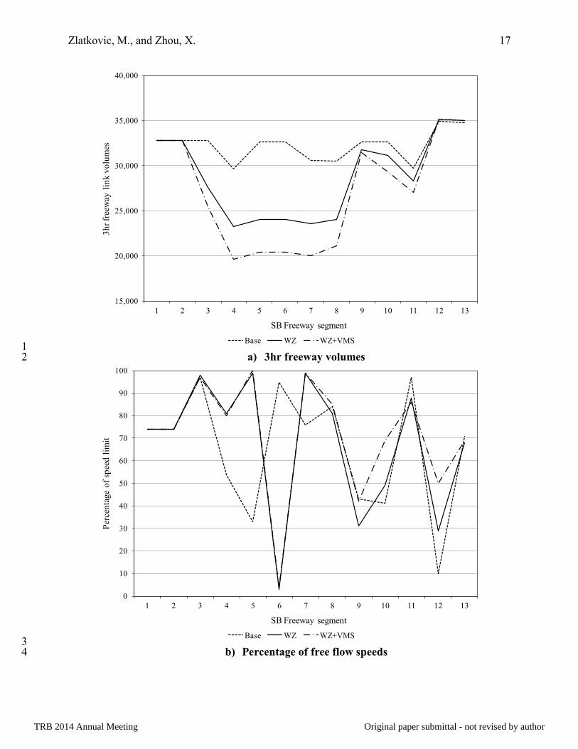
freeway and signalized intersections. Figure 5 a) and b) shows comparisons of freeway volumes 15

and speeds as a percentage of the free-flow speed, given for SB freeway segments. Figure 5 c) 16

shows a comparison of the average signalized intersection delays. 17

18

R² = 0.97

0

5,000

10,000

15,000

20,000

25,000

30,000

0 5,000 10,000 15,000 20,000 25,000 30,000

Sim

ula

ted

3h

r v

olu

mes

Observed 3hr volumes



1 a) 3hr freeway volumes 2

3 b) Percentage of free flow speeds 4

15,000

20,000

25,000

30,000

35,000

40,000

1 2 3 4 5 6 7 8 9 10 11 12 13

3h

r fr

eew

ay l

ink

vo

lum

es

SB Freeway segment

Base WZ WZ+VMS

0

10

20

30

40

50

60

70

80

90

100

1 2 3 4 5 6 7 8 9 10 11 12 13

Per

cen

tage

of

spee

d l

imit

SB Freeway segment

Base WZ WZ+VMS



1 c) Average intersection delays 2

FIGURE 5 Work zone analysis results on freeway and intersection level. 3 4

The work zone impacts are present on both levels. In both WZ scenarios, the freeway 5

volumes changed along the whole stretch of the freeway. The reduced capacity and speed within 6

the work zone area cause time-dependent changes in traffic patterns reported by the DTA model. 7

The implementation of VMS further reduces the freeway volumes. The drop in freeway volumes 8

starts at segment 2, which is located at the 3300 S ramp, where vehicles exit the freeway in 9

search for alternate routes. The volumes are lower throughout the entire work zone, and they 10

start to increase after the ramp at 4500 S. Once passed the 5300 S ramp, the volumes in the WZ 11

scenarios return to regular levels, meaning that all the vehicles that used alternate routes returned 12

to the freeway. 13

The speeds in the base scenario drop significantly at segments 4 and 5, which are the 14

segments after the 3300 S on-ramp. In the WZ scenarios speeds at these segments are much 15

higher, because of the significantly lower volumes after the 3300 S ramp. However, the speeds 16

within the work zone affected area (within and around segment 6) drop significantly in both WZ 17

scenarios. The speeds in the WZ + VMS scenario are slightly higher in the segments following 18

the work zone. The speeds in the three scenarios converge to the same value after the 5300 S 19

ramp. These results can be used to assess the work zone impacts on freeway traffic. 20

The analysis of delays at signalized intersections through QEM shows the impacts that a 21

freeway work zone has on the adjacent arterial network. Signalized ramps experience the most 22

increase in delays, which is higher in both WZ scenarios. The increase in delays at intersections 23

just east and west of the freeway and along the adjacent arterials is still significant. On average, 24

with QEM optimization for the new volumes, the delays for the 40 intersections were increased 25

about 12% in the WZ scenario. Figure 5 c) also shows significantly higher delays at critical 26

0

20

40

60

80

100

120

140

160

180

200

220

44

04

44

12

44

13

44

14

44

15

44

17

44

23

44

27

44

29

44

31

44

34

44

42

44

45

46

08

46

11

46

14

46

16

46

18

47

25

47

26

47

27

47

31

47

33

47

50

48

06

48

13

48

17

48

22

48

24

48

26

48

28

49

23

49

24

49

26

49

32

49

36

53

34

54

56

57

62

57

84

Av

erag

e in

ters

ecti

on

del

ay p

er v

ehic

le (

s)

Intersection code number

Base WZ WZ+VMS Delay w/out QEM signal optimization



intersections without the QEM optimization, increasing from 30% to almost 500% when 1

compared to the Base scenario. The VMS implementation also has impacts on arterial 2

operations, and the delays are in this case just slightly higher than in the Base scenario. QEM 3

provides detailed information for all signalized intersections, allowing much better assessments 4

of their performance. 5

6

6. CONCLUSIONS 7

Coupling DTA and traffic signal control models is a complex problem, and it has been a focus of 8

numerous research efforts. This paper presents one solution to the problem, where a DTA model, 9

for example DTALite used in our system implementation, is tightly coupled with a QEM Excel-10

based signal timing estimation tool. The two models operate in a continuous feedback loop in 11

each consecutive iteration until the convergence threshold is achieved. In each iteration, the 12

mesoscopic DTA package passes the intersection geometry and current paths to QEM, which 13

performs signal timing estimation and determines movement capacities, and sends them back to 14

the DTA package for next iteration. This framework provides detailed output data on multiple 15

network levels. A simple network that demonstrates the operation of the feedback loop and the 16

convergence of the two models is first presented, and then the framework is tested on a real-17

world network with a work zone implementation. 18

The results presented in this paper show promising results in coupling DTA and signal 19

control through the designed framework. The current application becomes stable after about 30 20

iterations, when the network parameters converge, with minimal changes in consecutive 21

iterations. The results from a real-world work zone example show that this application can 22

successfully be used to assess impacts of any events that disrupt normal traffic operations and 23

cause route switching on multiple levels, including signalized intersections. Future research 24

efforts will be focused on improving the current models, as well as developing a user-friendly 25

web-based GUI for easier data inputs and visualizations. 26

27

ACKNOWLEDGEMENT 28

The second author of this paper is partially supported through a FHWA research project titled 29

“Effective Integration of Analysis Modeling and Simulation Tools”. Special thanks to our 30

colleagues Brandon Nevers and other engineers at Kittelson & Associates, Inc. for their 31

constructive comments. The authors express their gratitude to the Mountain Plains Consortium 32

University Transportation Center that provided funds and assistance for this study. The work 33

presented in this paper remains the sole responsibility of the authors. 34

35

REFERENCES 36

1. Mahmassani, H. S. Dynamic Network Traffic Assignment and Simulation Methodology for 37

Advanced System Management Applications. In Networks and Spatial Economics, Vol. 12, 38

2001, pp. 267-292. 39

2. Abdelfatah, A. S. and H. S. Mahmassani. System Optimal Time-Dependent Path 40

Assignment and Signal Timing in Traffic Network. In Transportation Research Record: 41

Journal of the Transportation Research Board, No. 1645, Transportation Research Board 42

of the National Academics, Washington, D.C., 1998, pp. 185-193. 43



3. Sun, D., R. F. Benekohal, and S. T. Waller. Bi-level Programming Formulation and 1

Heuristic Solution Approach for Dynamic Traffic Signal Optimization. In Computer-Aided 2

Civil and Infrastructure Engineering No. 21, 2006, pp. 321-333. 3

4. Goodchild, M.F. Geographical Information Science. In International Journal of 4

Geographical Information Systems No. 6, 1992, pp. 31-45. 5

5. Nyerges, T.L. Coupling GIS and Spatial Analytical Models. In Proceedings of the 5th

6

International Symposium on Spatial Data Handling, Vol. 2, 1992, pp. 534-543. 7

6. Smith, M. J., and M. O. Ghali. The Dynamics of Traffic Assignment and Traffic Control: A 8

Theoretical Study. In Transportation Research No. 24B, 1990, pp. 409–422. 9

7. Smith, M. J., and M. O. Ghali. Dynamic Traffic Assignment and Dynamic Traffic Control. 10

Presented at 11th

International Symposium on Traffic and Transportation Theory. 11

Yokohama, Japan, 1990. 12

8. Gartner, N. H., and C Stamatiadis. Integration of Dynamic Assignment with Real-Time 13

Traffic Adaptive Control. In Transportation Research Record: Journal of the 14

Transportation Research Board, No. 1644, Transportation Research Board of the National 15

Academics, Washington, D.C., 1997, pp. 150–56. 16

9. Chen, O., and M. E. Ben-Akiva. Game-theoretic formulations of the interactions between 17

dynamic traffic control and dynamic traffic assignment. In Transportation Research 18

Record: Journal of the Transportation Research Board, No. 1617, Transportation Research 19

Board of the National Academics, Washington, D.C., 1998, pp. 179-188. 20

10. Ukkusuri, S., K. Doan., and H. M. Abdul Aziz. A Bi-level Formulation for the Combined 21

Dynamic Equilibrium based Traffic Signal Control. In Procedia - Social and Behavioral 22

Sciences No. 80, 2013, pp. 729-752. 23

11. Highway Capacity Manual 2010, Transportation Research Board of the National 24

Academies, Washington, D.C., 2010. 25

12. Koonce, P., et al. Traffic Signal Timing Manual. Publication FHWA- HOP-08-024. 26

FHWA, U.S. Department of Transportation, 2008. 27

13. Utah Department of Transportation. Signalized Intersection Design Guidelines. UDOT, 28

2012. 29

14. Lu C, Zhou, X and Zhang K. Dynamic Origin-Destination Demand Flow Estimation under 30

Congested Traffic Conditions. In Transportation Research Part C. Volume 34, 2013, pp. 31

16–37 32


effective coupling of signal timing estimation model and ...docs.trb.org/prp/14-4957.pdf · 1...

Documents