This article was downloaded by: [UNICAMP]On: 19 August 2013, At: 10:03Publisher: Taylor & FrancisInforma Ltd Registered in England and Wales Registered Number: 1072954 Registeredoffice: Mortimer House, 37-41 Mortimer Street, London W1T 3JH, UK

GIScience & Remote SensingPublication details, including instructions for authors andsubscription information:http://www.tandfonline.com/loi/tgrs20

Effect of sugarcane-planting rowdirections on ALOS/PALSAR satelliteimagesMichelle Cristina Araujo Picoli a , Rubens Augusto CamargoLamparelli b , Edson Eyji Sano c , Jefferson Rodrigo Batista deMello d & Jansle Vieira Rocha ea Brazilian Bioethanol Science and Technology Laboratory , CTBE/CNPEM , PO Box 6170, Campinas , São Paulo , Brazil , 13083-970b Interdisciplinary Center of Energy Planning , State Universityof Campinas , PO Box 6166, Campinas , São Paulo , Brazil ,13083-896c Cerrados Agricultural Research Center, Brazilian AgriculturalResearch Organization, Embrapa Cerrados , PO Box 08223,Planaltina , Federal District , Brazil , 73301-970d Department of Geotechnology , Raízen S.A , PO Box 1331,Piracicaba , São Paulo , Brazil , 13405-970e Department of Planning and Sustainable Rural Development –State University of Campinas – UNICAMP/FEAGRI , PO Box 6011,Campinas , São Paulo , Brazil , 13083-875Published online: 02 Jul 2013.

To cite this article: Michelle Cristina Araujo Picoli , Rubens Augusto Camargo Lamparelli , EdsonEyji Sano , Jefferson Rodrigo Batista de Mello & Jansle Vieira Rocha (2013) Effect of sugarcane-planting row directions on ALOS/PALSAR satellite images, GIScience & Remote Sensing, 50:3,349-357

To link to this article: http://dx.doi.org/10.1080/15481603.2013.808457

PLEASE SCROLL DOWN FOR ARTICLE

Taylor & Francis makes every effort to ensure the accuracy of all the information (the“Content”) contained in the publications on our platform. However, Taylor & Francis,our agents, and our licensors make no representations or warranties whatsoever as tothe accuracy, completeness, or suitability for any purpose of the Content. Any opinionsand views expressed in this publication are the opinions and views of the authors,and are not the views of or endorsed by Taylor & Francis. The accuracy of the Content

should not be relied upon and should be independently verified with primary sourcesof information. Taylor and Francis shall not be liable for any losses, actions, claims,proceedings, demands, costs, expenses, damages, and other liabilities whatsoever orhowsoever caused arising directly or indirectly in connection with, in relation to or arisingout of the use of the Content.

This article may be used for research, teaching, and private study purposes. Anysubstantial or systematic reproduction, redistribution, reselling, loan, sub-licensing,systematic supply, or distribution in any form to anyone is expressly forbidden. Terms &Conditions of access and use can be found at http://www.tandfonline.com/page/terms-and-conditions

Dow

nloa

ded

by [

UN

ICA

MP]

at 1

0:03

19

Aug

ust 2

013

Effect of sugarcane-planting row directions on ALOS/PALSARsatellite images

Michelle Cristina Araujo Picolia*, Rubens Augusto Camargo Lamparellib,Edson Eyji Sanoc, Jefferson Rodrigo Batista de Mellod and Jansle Vieira Rochae

aBrazilian Bioethanol Science and Technology Laboratory, CTBE/CNPEM, PO Box 6170,Campinas, São Paulo, Brazil, 13083-970; bInterdisciplinary Center of Energy Planning, StateUniversity of Campinas, PO Box 6166, Campinas, São Paulo, Brazil, 13083-896; cCerradosAgricultural Research Center, Brazilian Agricultural Research Organization, Embrapa Cerrados,PO Box 08223, Planaltina, Federal District, Brazil, 73301-970; dDepartment of Geotechnology,Raízen S.A., PO Box 1331, Piracicaba, São Paulo, Brazil, 13405-970; eDepartment of Planning andSustainable Rural Development – State University of Campinas – UNICAMP/FEAGRI, PO Box6011, Campinas, São Paulo, Brazil, 13083-875

(Received 12 July 2012; final version received 22 May 2013)

This study investigated the effects of sugarcane-planting row directions in the HH- andVV-polarized, ALOS/PALSAR imageries. Twenty sugarcane fields from São PauloState, Brazil, were classified into rows parallel and rows perpendicular to the rangedirection of the satellite. Backscattering coefficients (σ°) from 10 images were ana-lyzed. For HH polarization, σ° values from fields with perpendicular rows were higherthan those from parallel rows (~1.2 dB). For HV polarization, there was no statisticallysignificant difference. Therefore, HV-polarized PALSAR images are preferable forproducing maps of cultivated areas with sugarcane or to discriminate sugarcanevarieties, among other applications.

Keywords: synthetic aperture radar (SAR); sugarcane; row directions; L-band

Introduction

Although optical remote-sensing images are often used for agricultural monitoring(e.g., Fortes and Demattê 2006; Abdel-Rahman and Ahmed 2008), they presentrestrictions in regions with persistent cloud cover. Moreover, optical data are relatedonly to the top millimeters of a canopy, and the effects of solar illumination andsolar azimuth angle need to be taken into consideration. An alternative is to usesynthetic aperture radar (SAR) data because they can obtain images of the Earth’ssurface regardless of cloud cover conditions (Paradella et al. 2005; Radarsat-2 2013);moreover. it presents very high synergies with optical remote sensing (Jiaguo et al.2004). Another advantage of SAR sensors is the possibility of data acquisition infour different polarization modes – (HH (horizontal transmit and horizontal receive),HV (horizontal transmit and vertical receive), VH (vertical transmit and horizontalreceive), and VV (vertical transmit and vertical receive)) – which allows better targetdiscrimination and image classification (Yun et al. 1995; McNairn and Brisco 2004;McNairn, Hochheim, and Rabe 2004).

*Corresponding author. Email: michelle.picoli@bioetanol.org.br

GIScience & Remote Sensing, 2013Vol. 50, No. 3, 349–357, http://dx.doi.org/10.1080/15481603.2013.808457

© 2013 Taylor & Francis

Dow

nloa

ded

by [

UN

ICA

MP]

at 1

0:03

19

Aug

ust 2

013

Spectral signatures of sugarcane (Saccharum spp.) in the microwave region arestill poorly understood because of a limited research. One exception is the work ofBaghdadi et al. (2009) and Baghdadi, Todoroff, and Zribi (2011), who concluded thatthe data obtained by L-band and HH- and HV-polarized SAR systems from areasplanted with sugarcane in Reunion Island, east of Madagascar, were highly correlatedwith height measurements. They also reported a strong correlation between theHH-polarized backscatter coefficient (σ°) and the normalized difference vegetationindex (NDVI) derived from the maturation and harvesting stages. At the maturationphase, the σ° values presented a sharp decline related to the decrease of the plantwater content. Haraguchi et al. (2010) have used Palsar data in monitoring sugarcanecrop during its vegetative cycle, but there were no findings of a relationship between abackscatter and the crop parameters such as plant height, density, and leaf numbers.Lin et al. (2009), studying sugarcane plantations in Guangdong Province, China,noticed a high correlation between leaf area index (LAI) and C-band HV/HH-ratioedσ°. They highlighted the importance of image analysis obtained in the seedling andmaturation stages. In these phases, the σ° values from sugarcane fields were highlydistinct from the σ° of the surrounding targets.

Other studies have emphasized the use of L-band data because of their close relation-ship with plant biomass (Brisco et al. 1992; Pampaloni et al. 1997; Baghdadi et al. 2009).Paloscia (1998), by analyzing the performance of C-, L-, and P-band σ° values to estimatethe LAI of wheat, corn, and alfalfa, concluded that the best results were obtained by theL-band data with a HV polarization. Significant differences in σ° were reported by Paris(1983), Moran et al. (1998) and Silva et al. (2009) in studies involving soy, corn, cotton,coffee, potato, carrot, beet, onion, and wheat with different planting row directions. Thisstudy aimed to understand the influence of sugarcane-planting row directions in theL-band and HH- and HV-polarized ALOS/PALSAR imageries.

Materials and methods

Study area

The study area comprised sugarcane fields in the northeastern region of São Paulo State, in themunicipalities of Dobrada and Guariba (between 20° 28′ and 21° 38′ south latitude and between48° 13′ and 48° 22′ west longitude), near the municipalities of Jaboticabal (north) andAraraquara (southeast). The climate is tropical. According to the 1971–2000 climatologicaltime series, January to March are the wettest months (607 mm on average), and January andFebruary are the hottest months (24.3°C on average). July to September are the driest months(118.2 mm on average), and June is the coolest month (18.6°C on average) (UNESP 2011). Theelevation ranges from 500 to 800 m, while the slope varies from zero to 8% (Oliveira et al.1999). Oxisols are the dominant soil type in the region (Martorano et al. 1999).

The study area represents more than 35,000 hectares of sugarcane of 23 varieties withearly (harvesting in April and May), intermediate (harvesting in May to July), and late(harvesting in July to September) growing cycles. Early varieties can have either12-month (year sugarcane) or 18-month (year-and-a-half sugarcane) growing periods.After the first harvest, the cycle reaches 12 months, after which it is called ratoonsugarcane or stubble crop. The same crop can be harvested five to seven times (Rudorffet al. 2010). The appropriate variety is chosen based on local biophysical conditions (soil,climate, and plant characteristics). According to Prado et al. (1998) and Prado (2005),areas for sugarcane cultivation are often classified into five categories – from A (bestsituation) to E (worst situation).

350 M.C.A. Picoli et al.

Dow

nloa

ded

by [

UN

ICA

MP]

at 1

0:03

19

Aug

ust 2

013

This research considered only plots with the RB86-7515 variety because it was themost representative in the study site. This variety presents a rapid growth rate, a tallcanopy, a strong upright growing trend, a high density of stems, a dominant purple-greencolor, and an intermediate growing cycle. The variety is also drought tolerant and has ahigh saccharose content and high productivity (Hoffmann et al. 2008).

Database

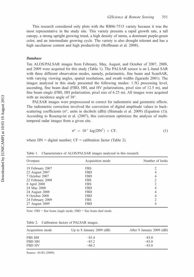
Ten ALOS/PALSAR images from February, May, August, and October of 2007, 2008,and 2009 were acquired for this study (Table 1). The PALSAR sensor is an L-band SARwith three different observation modes, namely, polarimetric, fine beam and ScanSAR,with varying viewing angles, spatial resolutions, and swath widths (Igarashi 2001). Theimages analyzed in this study presented the following modes: 1.5G processing level,ascending, fine beam dual (FBD, HH, and HV polarizations, pixel size of 12.5 m), andfine beam single (FBS, HH polarization, pixel size of 6.25 m). All images were acquiredwith an incidence angle of 38°.

PALSAR images were preprocessed to correct for radiometric and geometric effects.The radiometric correction involved the conversion of digital amplitude values to back-scattering coefficients (σ°, units in decibels (dB)) (Shimada et al. 2009) (Equation (1)).According to Rosenqvist et al. (2007), this conversion optimizes the analysis of multi-temporal radar images from a given site.

σ° ¼ 10 � logðDN2Þ þ CF; (1)

where DN = digital number; CF = calibration factor (Table 2).

Table 1. Characteristics of ALOS/PALSAR images analyzed in this research.

Overpass Acquisition mode Number of looks

19 February 2007 FBS 222 August 2007 FBD 47 October 2007 FBD 422 February 2008 FBS 28 April 2008 FBS 224 May 2008 FBD 424 August 2008 FBD 49 October 2008 FBD 424 February 2009 FBS 227 August 2009 FBD 4

Note: FBS = fine beam single mode, FBD = fine beam dual mode.

Table 2. Calibration factors of PALSAR images.

Acquisition mode Up to 8 January 2009 (dB) After 9 January 2009 (dB)

FBS HH −83.4 −83.0FBD HH −83.2 −83.0FBD HV −80.2 −83.0

Source: AUIG (2009).

GIScience & Remote Sensing 351

Dow

nloa

ded

by [

UN

ICA

MP]

at 1

0:03

19

Aug

ust 2

013

The geometric correction of the PALSAR images was conducted based on the LandsatETM+ GeoCover image acquired on 23 March 2001, and available at the website of theUniversity of Maryland, USA (http://glcf.umiacs.umd.edu/data/landsat/). The images wereregistered to the UTM projection system, the WGS84 datum and the 23S time zone.

A set of 20 plots was classified as parallel or perpendicular to the sensor’s lookdirection (Figure 1). This classification was based on 5-m equidistance contour lines ofthe study area (1:10.000 scale) provided by the Bonfim Mill and derived from an ALOS/VNIR image (spatial resolution: 10 m) obtained on 8 February 2008, and from aQuickBird optical image available in the Google Earth™ program (overpass: April2008). The time differences between the PALSAR, AVNIR, and QuickBird overpasseswere considered negligible, as the sugarcane plots were planted in 2004 and remained inthe field for at least five years.

Mean σ° values were calculated for the plots presenting the planting of rows paralleland perpendicular to the direction of the emitted SAR signals. To better understand thetemporal behavior of the backscatter signals from sugarcane plantations, was analyzedprecipitation data. The precipitation is directly related to the soil moisture content and isone of the surface parameters that strongly influence the intensity of backscattered energy.These data were provided by the Bonfim Mill group. The average σ° values from theplanting rows perpendicular and parallel relative to the sensor look direction wereanalyzed statistically using a non-parametric Mann-Whitney test (Mann and Whitney1947) at significance level of 5%.

Results and discussion

Ten plots were classified as having parallel planting rows and 10 as having perpendicularrows. The relative distance between the planting rows was 1.4 m at the beginning of thecycle for the perpendicular-viewing plots. The relative distance between plants in thesame line was approximately 0.2 m at the beginning of the season for the parallel-viewingplots (Figure 2). These distances tended to decrease as the sugarcane grew and clumpsincreased.

For HH polarization, the mean σ° values for the perpendicular plots were 0.7–2.3 dBhigher than those from parallel plots. For HV polarization, there was no difference in σ°values at a significance level of 5%. Wegmüller et al. (2011) also noted that the plantingrow directions found in potato, carrot, beet, onion and wheat crops had an influence onSAR signals obtained by HH and VV polarizations, but not by HV or VH polarizations.

Lookdirection

A

Asc

endi

ng o

rbit

A

B BA: Parallel plots

B: Perpendicular plots

Figure 1. Diagram used to classify sugarcane plots into parallel and perpendicular to the sensor’slook direction.Source: Adapted from Silva et al. (2009).

352 M.C.A. Picoli et al.

Dow

nloa

ded

by [

UN

ICA

MP]

at 1

0:03

19

Aug

ust 2

013

HV-polarized data are more closely correlated with LAI or biomass, as noted by Paloscia(1998) and Simões, Rocha, and Lamparelli (2005).

The mean σ° values for the plots planted with parallel and perpendicular rows andprecipitation data are shown in Figure 3, because the relations of soil and plant to waterplay an important role on the backscattering signal (Formaggio, Epiphanio, and Simões2001). In the image acquired on 9 October 2008 (10 months of the growing cycle), wewould expect lower σ° values because of the maturation phase of the plant and thedominant dry conditions at this time of year. However, the rainfall accumulated byOctober 8 was relatively high, at 43 mm (Figure 3). This rainfall accumulation mayhave caused an increase of the dielectric constant of the plant, consequently increasing theσ° values. For the image acquired in February 2009 (two months of the growing cycle),

1.40 m

(a) (b)

0.20 m

Figure 2. Average spaces between sugarcane planting rows (a) and between plants in the samerow (b).

3 M

9 M

11 M 2 M

4 M

5 M

8 M

10 M 2 M

8 M

0

–2

–4

–6

–8

–10

Bac

ksca

tteri

ng (

dB)

–12

–14

–16

–18

–20

125

100

75

50

Acc

umul

ated

rai

nfal

l (m

m)

25

150

0

Accumulated rainfall Parallel HH Perpendicular HHMonth

2007 2008 2009

Parallel HV Perpendicular HV

Figure 3. Mean σ° from the sugarcane plots, and rainfall data from the study area.Note: M – month.

GIScience & Remote Sensing 353

Dow

nloa

ded

by [

UN

ICA

MP]

at 1

0:03

19

Aug

ust 2

013

however, the plots showed low σ° values because of a dry spell event that occurred nearthe time of the satellite overpass. The results indicate a strong influence of accumulatedrainfall of backscatter, seeing that the σ° values are directly related to the soil water.

The effect of the planting rows in the HH-polarized PALSAR data was noticed untilthe eighth month of age (Table 3). In the image acquired in October 2008 (10 months ofage, average plant height of approximately 3.5 m), the σ° values from the parallel plotswere similar to those from the perpendicular plots, probably because sugarcane wasalready completely covering the soil surface.

Overall, the plots with young plants (two or three months of age) were more sensitiveto the effects of the planting rows because of the characteristics of the plant management(Figure 4). The backscatter values from the perpendicular plots were higher than those

Table 3. A Mann–Whitney test was used to compare sugarcane’s plots parallel and perpendicularto the satellite’s look direction (α = 0.05) and the descriptive summary statistics (mean and standarddeviation).

Satellite overpass PolarizationAge of

plant (months)Parallel plots(µ and σ)

Perpendicular plots(µ and σ) P-value

19 February 2007 HH 3 −11.56 (σ = 0.62) −9.29 (σ = 0.56) 0.000222 August 2007 HH 9 −12.83 (σ = 0.66) −12.48 (σ = 0.92) 0.5966a

22 August 2007 HV 9 −15.45 (σ = 0.96) −15.78 (σ = 1.54) 0.2121a

7 October 2007 HH 11 −15.78 (σ = 1.02) −15.11 (σ = 1.44) 0.3847a

7 October 2007 HV 11 −17.49 (σ = 1.25) −17.66 (σ = 1.95) 0.3256a

22 February 2008 HH 2 −11.15 (σ = 1.18) −8.91 (σ = 0.91) 0.00138 April 2008 HH 4 −11.16 (σ = 0.59) −9.10 (σ = 0.68) 0.000224 May 2008 HH 5 −12.26 (σ = 0.66) −11.51 (σ = 0.58) 0.037624 May 2008 HV 5 −16.57 (σ = 0.87) −15.94 (σ = 0.86) 0.1121a

24 August 2008 HH 8 −13.52 (σ = 0.53) −12.30 (σ = 0.73) 0.002824 August 2008 HV 8 −16.72 (σ = 0.72) −16.22 (σ = 0.98) 0.2413a

9 October 2008 HH 10 −10.46 (σ = 0.54) −9.77 (σ = 0.50) 0.00919 October 2008 HV 10 −12.46 (σ = 0.97) −12.80 (σ = 0.76) 0.3913a

24 February 2009 HH 2 −14.56 (σ = 0.40) −13.50 (σ = 0.63) 0.003927 August 2009 HH 8 −11.02 (σ = 0.55) −10.32 (σ = 0.40) 0.014527 August 2009 HV 8 −15.42 (σ = 0.98) −15.87 (σ = 0.72) 0.5636a

Note: aNot significant at 5%.

(a) (b) (c)

Figure 4. PALSAR HH-polarized image from 22 February 2008 (a), QuickBird optical imageavailable in the Google Earth™ program from April 2008 (b) and a PALSAR HH-polarized imagefrom 8 April 2008, (c) overpasses. Parallel plots are outlined in red, and perpendicular plots areoutlined in green. The image scene is 2.9 km.

354 M.C.A. Picoli et al.

Dow

nloa

ded

by [

UN

ICA

MP]

at 1

0:03

19

Aug

ust 2

013

from the parallel plots. After a mechanical harvesting, the straws are left on the soilsurface (~10 cm thickness) to prevent the development of shoots. After approximatelyseven days, the straws start to clump, forming windrows along the planting rows. Thistype of management leads to a succession of small clumps with a height of approximately15–20 cm aligned along the row direction, increasing the terrain’s directional roughness(Figure 5) and, consequently, increasing the σ° values, especially for the perpendicularplots. This result may have occurred because the sugarcane plants are regularly spaced inthe range direction and are aligned with the wave fronts. Thus, the reflection of each plantwill contribute coherently with the reflection of the other scatterers. This phenomenon isknown as Bragg scattering. The same finding was also obtained by Formaggio,Epiphanio, and Simões (2001).

Conclusions

The results indicate that in some cases there are statistical differences between L-band σ°values. These differences are caused by the effects of different planting row directions(parallel and perpendicular to the sensor’s look direction). These differences need to betaken into account, for instance, in works aiming to discriminate sugarcane varieties andto estimate sugarcane productivity from SAR data.

HH polarization was more influenced by the planting row direction than HV polariza-tion, mainly for aged plants (>eight months). To obtain more accurate maps of sugarcaneplantations or to monitor sugarcane productivity, we recommend giving preference toHV-polarized images. As an ongoing research, we recommend designing and validatingspecific image processing techniques that have the potential to reduce planting row effectsin the HH-polarized ALOS/PALSAR imageries.

Figure 5. Panoramic field photo obtained on 14 May 2010, illustrating a typical directional terrainroughness found in the study area after sugarcane harvesting.

GIScience & Remote Sensing 355

Dow

nloa

ded

by [

UN

ICA

MP]

at 1

0:03

19

Aug

ust 2

013

AcknowledgementsThe authors would like to thank FAPESP (Project Number 2008/06043-5) and CNPq for financialsupport. Dr. Laura Hess provided ALOS/PALSAR images. Fernando Benvenuti (Raízen) provideduseful suggestions and support in gathering the field data.

ReferencesAbdel-Rahman E. M., and F. B. Ahmed. 2008. “The Application of Remote Sensing Techniques to

Sugarcane (Saccharum spp. Hybrid) Production: A Review of the Literature.” InternationalJournal of Remote Sensing 29 (13): 3753–3767.

AUIG (Alos User Interface Gateway). 2009. PALSAR: Calibration factor updated. Accessed June 8,2009. https://auig.eoc.jaxa.jp/auigs/en/doc/an/20090109en_3.html

Baghdadi, N., N. Boyer, P. Todoroff, M. Hajj, and A. Bégué. 2009. “Potential of SAR SensorsTerraSAR-X, ASAR/ENVISAT and PALSAR/ALOS for Monitoring Sugarcane Crops onReunion Island.” Remote Sensing of Environment 113 (8): 1724–1738.

Baghdadi, N., P. Todoroff, and M. Zribi. 2011. “Multitemporal Observations of Sugarcane byTerraSAR-X Sensor.” IEEE International Geoscience and Remote Sensing Symposium,Vancouver, BC, July 24–29, 1401–1404.

Brisco, B., R. J. Brown, J. G. Gairns, and B. Snider. 1992. “Temporal Ground-Based ScatterometerObservations of Crops in Western Canada.” Canadian Journal of Remote Sensing 18 (1):14–22.

Formaggio, A. R., J. C. N. Epiphanio, and M. S. Simões. 2001. “Radarsat Backscattering from anAgricultural Scene.” Pesquisa Agropecuária Brasileira 36 (5): 823–830.

Fortes, C., and J. A. M. Demattê. 2006. “Discrimination of Sugarcane Varieties Using Landsat 7ETM+ Spectral Data.” International Journal of Remote Sensing 27 (7): 1395–1412.

Haraguchi, M., Y. Akamatsu, T. Morita, C. Kobayashi, and M. Kawai. 2010. “Biofuel FieldMapping and Growth Monitoring Using Palsar Data.” International Archives of thePhotogrammetry, Remote Sensing and Spatial Information Science XXXVIII, Part 8: 572–575.

Hoffmann, H. P., E. G. D. Santos, A. I. Bassinello, and M. A. S. Vieira. 2008. Variedades RB deCana-de-Açúcar. Araras: Universidade Federal e São Carlos.

Igarashi, T. 2001. “Alos Mission Requirement and Sensor Specifications.” Advances in SpaceResearch 28 (1): 127–131.

Jiaguo, Q., W. Cuizhen, I. Yoshio, Z. Renduo, and G. Wei. 2004. “Synergy of Optical and RadarRemote Sensing in Agricultural Applications.” In Proceedings of the SPIE on Ecosystems’Dynamics, Agricultural Remote Sensing and Modeling, and Site-Specific Agriculture, edited byW. Gao, and R. David. Vol. 5153, 153–158. Accessed May 13, 2013. http://spie.org/

Lin, H., J. Chen, Z. Pei, S. Zhang, and X. Hu. 2009. “Monitoring Sugarcane Growth UsingENVISAT ASAR Data.” IEEE Transactions on Geoscience and Remote Sensing 47 (8):2572–2580.

Mann, H. B., and D. R. Whitney. 1947. “On a Test of Whether One of Two Random Variables isStochastically Larger than the Order.” The Annals of Mathematical Statistics 18 (1): 50–60.

Martorano, L. G., L. R. Angelocci, C. A. Vettorazzi, and R. O. A. Valente. 1999. “ZoneamentoAgroecológico para a Região de Ribeirão Preto Utilizando um Sistema de InformaçõesGeográficas.” Scientia Agricola 56 (3): 739–747.

McNairn, H., and B. Brisco. 2004. “The Application of C-Band Polarimetric SAR for Agriculture:A Review.” Canadian Journal of Remote Sensing 30 (3): 525–542.

McNairn, H., K. Hochheim, and N. Rabe. 2004. “Applying Polarimetric Radar Imagery forMapping the Productivity of Wheat Crops.” Canadian Journal of Remote Sensing 30 (3):517–524.

Moran, M. S., A. Vidal, D. Troufleau, Y. Inoue, and T. A. Mitchell. 1998. “Ku- and C-Band SAR forDiscriminating Agricultural Crop and Soil Conditions.” IEEE Transactions on Geoscience andRemote Sensing 36 (1): 265–272.

Oliveira, J. B., M. N. Camargo, M. Rossi, and B. Calderano Filho. 1999. Mapa Pedológico doEstado de São Paulo – Legenda Expandida. Campinas: Instituto Agronômico de Campinas.

Paloscia, S. 1998. “An Empirical Approach to Estimating Leaf Area Index from MultifrequencySAR Data.” International Journal of Remote Sensing 19 (2): 359–364.

356 M.C.A. Picoli et al.

Dow

nloa

ded

by [

UN

ICA

MP]

at 1

0:03

19

Aug

ust 2

013

Pampaloni, P., G. Macelloni, S. Paloscia, and S. Sigismondi. 1997. “The Potential of C- and L-BandSAR in Assessing Vegetation Biomass: The ERS-1 and JERS-1 Experiments.” The 3rd ERSSymposium on Space at the Service of our Environment, Florence, March 17–21, 3: 1729–1733.

Paradella, W. R., A. R. Santos, P. Veneziani, and E. S. P. Cunha. 2005. “Radares Imageadores nasGeosciências: Estado da Arte e Perspectivas.” Revista Brasileira de Cartografia 57 (1): 56–62.

Paris, J. F. 1983. “Radar Backscattering Properties of Corn and Soybeans at Frequencies of 1.6, 4.75and 13.3 GHz.” IEEE Transactions on Geoscience and Remote Sensing, GE-21 (3): 392–400.

Prado, H. 2005. Ambientes de Produção de Cana-de-Açúcar na Região Centro-Sul doBrasil. Encarte Técnico. Informações Agronômicas, 110, June 2005. Accessed February25, 2010. http://www.ipni.net/ppiweb/brazil.nsf/87cb8a98bf72572b8525693e0053ea70/7759ddc6878ca7eb83256d05004c6dd1/$FILE/Encarte110.pdf

Prado, H., M. G. A. Landell, R. Rossetto, M. P. Campana, L. Zimback, and M. A. Silva. 1998.“Relation between Chemical Subsurface Conditions of Subsoils and Sugarcane Yield.” The 16thWorld Soil Science Congress, Montpellier, August 20–26, 1: 232.

RADARSAT-2. 2013. Canada’s Next Generation SAR Satellite. Accessed May 03, 2013. http://gs.mdacorporation.com/SatelliteData/Radarsat2/Radarsat2.aspx

Rosenqvist, A., M. Shimada, N. Ito, and M. Watanabe. 2007. “Alos Palsar: A Pathfinder Mission forGlobal-Scale Monitoring of the Environment.” IEEE Transactions on Geoscience and RemoteSensing 45 (11): 3307–3316.

Rudorff, B. F. T., D. A. Aguiar, W. F. Silva, L. M. Sugawara, M. Adami, and M. A. Moreira. 2010.“Studies on the Rapid Expansion of Sugarcane for Ethanol Production in São Paulo State(Brazil) using Landsat Data.” Remote Sensing 2 (4): 1057–1076.

Shimada, M., O. Isoguchi, T. Tadono, and K. Isono. 2009. “Palsar Radiometric and GeometricCalibration.” IEEE Transactions on Geoscience and Remote Sensing 47 (12): 3915–3932.

Silva, W. F., B. F. T. Rudorff, A. Formaggio, W. R. Paradella, and J. Mura. 2009. “Discrimination ofAgricultural Crops in a Tropical Semi-Arid Region of Brazil based on L-Band PolarimetricAirborne SAR Data.” ISPRS Journal of Photogrammetry and Remote Sensing 64 (5): 458–463.

Simões, M. S., J. V. Rocha, and R. A. C. Lamparelli. 2005. “Growth Indices and Productivity inSugarcane.” Scientia Agricola 62 (1): 23–30.

UNESP (Universidade Estadual Paulista Júlio de Mesquita Filho). Resenha Meteorológica doPeríodo 1971–2000. Jaboticabal. Accessed January 20, 2011. http://jaguar.fcav.unesp.br/portal_agromet/int_conteudo_sem_img.php?conteudo=180

Wegmüller, U., M. Santoro, F. Mattia, A. Balenzano, G. Satalino, P. Marzahn, G. Fischer, R.Ludwig, and N. Floury. 2011. “Progress in the Understanding of Narrow DirectionalMicrowave Scattering of Agricultural Fields.” Remote Sensing of Environment 115 (10):2423–2433.

Yun, S., G. Huadong, L. Hao, L. Junfei, and L. Xinqiao. 1995. “Effect of Polarization andFrequency using GlobeSAR Data Vegetation Discrimination.” Geocarto International 10 (3):71–78.

GIScience & Remote Sensing 357

Dow

nloa

ded

by [

UN

ICA

MP]

at 1

0:03

19

Aug

ust 2

013