effect of solder joint flux residue on medical guide wire
TRANSCRIPT

Effect of Solder Joint Flux Residue on Medical Guide Wire Performance
A Senior Project Presented to the Faculty of the Materials Engineering Department, California
Polytechnic State University, San Luis Obispo
In Partial Fulfillment of the Requirements for the Degree Bachelor of Science
by
Enlly Bugarin and Rebecca Lisberg
June 2019
© 2019
ii
Abstract
The effect of residual soldering flux on the mechanical properties of 304 stainless-steel core
medical guide wires was analyzed. A soldering process joins the metallic components of the
distal end of a medical guide wire product. Acidic soldering flux is used to prepare the surfaces
of the metallic substrates. Manufacturing protocol utilizes an ultrasonic bath to remove excess
flux from the soldered joints. Sample groups underwent different levels of cleaning: no cleaning,
partial cleaning, and full ultrasonic bath cleaning to obtain varying residual flux levels.
Experimental sample groups underwent corrosion acceleration in an environmental chamber at
37°C and 85% relative humidity for two 6-hour cycles. Control sample groups were maintained
at ambient temperature and humidity. Specimens were tensile tested using a gauge length of 25
cm and a crosshead rate of 10 mm/min on an Instron testing system. A 500-Newton (N) load-cell
and 50-N load-cell were used to test the control and experimental groups, respectively. The
average maximum loads at fracture obtained by the ambiently exposed samples were 19.52N,
20.1N, and 23.83N for the uncleaned, partially cleaned, and fully cleaned groups, respectively.
Experimental sample groups achieved average maximum loads of 13.54N, 13.91N, and 15.31N
for the uncleaned, partially cleaned, and fully cleaned groups, respectively. Scanning Electron
Microscopy (SEM) was utilized to analyze the presence of corrosion products in one specimen
per sample group.
Key words: solder joining, residual flux, corrosion, microvoid coalescence, guide wire, tip load,
materials engineering

iii
Acknowledgments
We would like to thank Professor Blair London for all of his guidance and support throughout
the project. We would also like to thank Dr. Puneet Gill and his team at Abbott Vascular for their
help with our samples and advice. Lastly, we would like to thank Professor Harding from the
Materials Engineering department and Professor Wyatt Brown from the Horticulture department
for their help with SEM and Environmental Exposure, respectively.

iv
Table of Contents 1Introduction........................................................................................................................................11.1ProblemStatement..................................................................................................................................11.2AbbottVascularInc.................................................................................................................................11.3MedicalGuideWires...............................................................................................................................21.3.1MetallicComponentsofaGuideWire..........................................................................................................5
1.4AbbottVascularSolderingProcess....................................................................................................61.4.1SolderFluxes...........................................................................................................................................................71.4.2Lead-FreeSolders.................................................................................................................................................71.4.3CorrosionatSolderJoints.................................................................................................................................91.4.4CleaningofResidualFlux...............................................................................................................................11
2ExperimentalProcedure.............................................................................................................122.1Safety..........................................................................................................................................................122.2DesignofExperiment............................................................................................................................122.3EnvironmentalExposure.....................................................................................................................132.4TensileTesting........................................................................................................................................142.5ScanningElectronMicroscopy...........................................................................................................162.5.1SamplePreparation..........................................................................................................................................16
3Results...............................................................................................................................................173.1EnvironmentalExposure.....................................................................................................................173.1.1EnvironmentalExposure–Humidity.......................................................................................................183.1.2EnvironmentalExposure–Temperature................................................................................................19
3.2TensileTesting........................................................................................................................................213.2.1GroupA..................................................................................................................................................................223.2.2GroupC...................................................................................................................................................................233.2.3GroupD..................................................................................................................................................................233.3.3Control....................................................................................................................................................................24
3.4ScanningElectronMicroscopy...........................................................................................................263.4.1GroupA..................................................................................................................................................................263.4.2GroupC...................................................................................................................................................................273.4.3GroupD..................................................................................................................................................................283.4.4Control....................................................................................................................................................................29
4Analysis.............................................................................................................................................30
5Conclusions......................................................................................................................................31
6References........................................................................................................................................32
7Appendix...............................................................................................................................................I

v
List of Figures
Figure 1. Guide wires are designed for placement through a catheter in the three main locations shown: femoral, brachial, and radial arteries [4]. .................................................................... 2
Figure 2. Example of a wire with proper trackability versus a wire with poor trackability that has prolapsed as the distal tip navigated a junction in the blood vessel[6]. ................................... 4
Figure 3. Example of various distal tip core profiles and their relation to the overall functional characteristics of the guide wire from Medtronic [7]. ............................................................. 4
Figure 4. Example of the distal end (red), center solder (green), and proximal solder (blue) of a guide wire. This wire utilizes multiple materials for both the outer coil and wire core [8]. ... 6
Figure 5. The rate of Sn dissolution in 0.05 M HNO3 increases when an Sn-Ag compound is present in comparison to a Sn-Pb compound; however, the rate of pure Sn dissolution is slowed by the Sn-Ag presence [20]. ........................................................................................ 9
Figure 6. The galvanic series for various metals, both 304 Stainless Steel and Gold are characterized by positive reduction potentials making them more cathodic; however, due to the difference in potentials Stainless Steel becomes the anode for the given corrosion cell [22]. ........................................................................................................................................ 10
Figure 7. Flowchart outlining each treatment group used in the experiment. Cleaning groups ranged from least clean to most clean from left to right. ....................................................... 13
Figure 8. Aluminum lining of the environmental chamber. Guide wires were secured by groups and separated by specimen. Temperature and humidity monitors (left) tracked parameters. 14
Figure 9. Mini Instron 55 tensile tester with a 500 N set-up. The proximal end of wire was clamped at the stationary jaws, while the distal end was clamped at the moving crosshead. 15
Figure 10. Wire clamping at proximal end (a) and distal solder (b). Alignment of the wire was crucial to obtain accurate results. Metal jaws of torque device (c) used to clamp solder joint. ............................................................................................................................................... 16
Figure 11. Relative humidity per sample group for environmental exposure testing cycle 1. Total testing time of 8 hours; 6 hours dwell time, 1-hour ramp-up, and 1-hour ramp-down. ........ 18
Figure 12. Relative humidity per sample group for environmental exposure testing cycle 2. Total testing time of 8 hours; 6 hours dwell time, 1-hour ramp-up, and 1-hour ramp-down. ........ 19
Figure 13. Temperature per sample group for environmental exposure testing cycle 1. Total testing time of 8 hours; 6 hours dwell time, 1-hour ramp-up, and 1-hour ramp-down. ........ 20
Figure 14. Temperature per sample group for environmental exposure testing cycle 2. Total testing time of 8 hours; 6 hours dwell time, 1-hour ramp-up, and 1-hour ramp-down. ........ 20
Figure 15. Box plots for maximum load data (N) from distal solder joint tensile testing of each treatment group. ..................................................................................................................... 21
Figure 16. Load [N] versus tensile strain [%] (extension) for ambient exposure group A samples. ............................................................................................................................................... 22

vi
Figure 17. Load [N] versus tensile strain [%] (extension) for elevated exposure group A samples. ............................................................................................................................................... 22
Figure 18. Load [N] versus tensile strain [%] (extension) for ambient exposure group C samples. ............................................................................................................................................... 23
Figure 19. Load [N] versus tensile strain [%] (extension) for elevated exposure group C samples. ............................................................................................................................................... 23
Figure 20. Load versus tensile strain [%] outputs for group D* exposed to ambient conditions. * specimens were handled with contaminated gloves and subject to water containing acidic flux. ........................................................................................................................................ 24
Figure 21. Load versus Load versus tensile strain [%] outputs for group D* exposed to elevated conditions. * specimens were handled with contaminated gloves and subject to water containing acidic flux ............................................................................................................ 24
Figure 22. Load versus tensile strain [%] outputs for control specimens exposed to ambient conditions. .............................................................................................................................. 25
Figure 23. Load versus tensile strain [%] outputs for control specimens exposed to elevated conditions. .............................................................................................................................. 25
Figure 24. Specimens with increased slippage shown with increased transparency to reduce clutter in chart. ....................................................................................................................... 26
Figure 25. Group A ambient (a) and elevated exposure (b). ........................................................ 27Figure 26. Elevated exposure, group A specimen after ultrasonic cleaning. An overall cup and
cone fracture surface (a) with a clear interface between low energy ductility and high energy microvoid coalescence (b). .................................................................................................... 27
Figure 27. Group C ambient (left) and elevated (right) exposure specimens. .............................. 28Figure 28. Group C ambient exposure displaying mixed modes of fracture. ............................... 28Figure 29. Group D specimens from ambient (left) and elevated (right) exposure treatments. ... 29Figure 30. Ambient exposed group D specimen at a higher magnification to show high and lower
energy ductile fracture surfaces. ............................................................................................ 29Figure 31. Control specimens from ambient (left) and elevated (right) exposure treatments. ..... 30

vii
List of Tables Table 1: Cleaning Procedures for each Level of Cleaning ........................................................... 12Table 2: Cycle 1 Average Dwell Time Temperature and Relative Humidity by Group. ............. 17Table 3: Cycle 2 Average Dwell Time Temperature and Relative Humidity by Group. ............. 17Table 4: Student’s t Test Results as calculated with JMP software. ............................................. 31

1
1 Introduction
1.1 Problem Statement Abbott Vascular utilizes a soldering process to join the metallic components on multiple
locations in many of their guide wire families. Their current soldering process uses an acidic flux
to clean the surface of each substrate; however, extended exposure to residual flux after cleaning
treatments has been found to corrode and potentially lead to premature failure of the soldering
joints and surrounding areas. The current technical challenge is preventing corrosion in their
medical grade guide wires. Available literature in this area has shown lead-free solders are most
susceptible to corrosion from acidic residues. For health and safety reasons, Abbott Vascular
utilizes two types of lead-free solders, and two solder fluxes. Each solder location undergoes an
initial pre-tinning, using Indalloy Flux II, and the solder process, using Alpha 90 Flux. To
address this problem, this project will assess the corrosion levels in guide wires exposed to
varying levels of residual flux for different environmental parameters. The specific goal of the
project is to determine the level of residual flux which will cause premature failure at worst case
storage conditions, high humidity and temperature. The guide wires will be exposed to extreme
temperature and humidity using a humidity/environmental chamber. To assess mechanical
properties after environmental exposure, tensile testing of fully assembled and the distal tip of
wires will be conducted. Failure analysis will consist of SEM to determine if residual flux or
corrosion products are present at the fracture site. The project will be completed by June 2019.
1.2 Abbott Vascular Inc.
Abbott Laboratories is an American health care company that was originally founded in
1888 by physician Wallace Calvin Abbott [1]. Abbott Laboratories is composed of four main
business divisions: Diagnostics, Nutrition, Generic Drugs, and Vascular [1,2]. In addition to
these four divisions, Abbott Laboratories also has a portfolio of diabetes care, medical optics and
other healthcare products[1]. Their cardiovascular sector, Abbott Vascular Inc., (Temecula, CA)
focuses on the development, manufacture, and sales of coronary, endovascular, vessel closure,
and structural heart devices [2]. These include coronary and peripheral guide wires, balloon
dilation catheters and drug-eluting stents, among many other products [3]. Through their
products, Abbott aims to help its customers live their best lives through good health.

2
1.3 Medical Guide Wires Guide wires are a medical device used in various cardiac and vascular intervention
procedures. They only require a large enough blood vessel and a catheter for entrance to the
desired artery (Figure 1) [4]. The wire allows a cardiac interventionist to guide the required tools
or devices to locations which would otherwise require highly invasive surgical operations to
access. These include, but are not limited to, the heart itself and major arteries surrounding the
heart such as the aorta.
Figure 1. Guide wires are designed for placement through a catheter in the three main locations shown: femoral, brachial, and radial arteries [4].
The design of guide wires is driven by the functional requirements. Multiple
characteristics of each wire are considered when planning an operation. Interventionalists may
utilize multiple guide wires when a single wire cannot deliver every required capabilities. Each
property is a tradeoff, therefore, specialty wires are often required in addition to an all-around
wire. Four main characteristics determine a wire’s use: trackability, torquability, flexibility, and
crossability. Trackability is the wire’s ability to navigate blood vessels both in loaded and
unloaded conditions. This can be refined further to steerability and trackability of a wire: the ease
of navigation through the blood vessel, and ease of the wire length to follow the distal tip,

3
respectively. Wires with higher levels of supportive strength perform better when loaded;
however, the less supportive wires typically display better trackability [5]. A failure in terms of
trackability is prolapse, a phenomena where the body of the wire does not follow the distal tip
and forms a knuckle as it enters a different blood vessel (Figure 2)[6]. This property often
corresponds to the mechanical properties, diameter, and distal tip taper profile of the core wire.
Torquability correlates to the wire’s ability to transfer stresses placed on the proximal end along
the length of the wire to the distal end. This property is an important safety consideration since a
wire with poor torquability will easily whip. Whipping refers to a wire that stores the torque
stresses from the proximal end, to a certain degree, until these stored stresses are released in the
form of a sudden, uncontrollable rotation of the distal tip. This sudden movement has the
potential to perforate or dissect the blood vessel. Flexibility is the wire’s ability to bend through
complex vessels while maintaining unstrained levels of trackability and torquability. This is
often controlled by the core material as well as distal tip design. Crossability is the wire’s ability
to push past a lesion or calcified region. The outer profile as well as tip strength of the wire
mainly contribute to this property. Wires with tapered ends and high tip load ratings allow the
greatest level of crossability (Figure 3). Wires displaying high levels of crossability are typically
only used to clear a calcified region, allowing passage for a less specialized wire [5].

4
Figure 2. Example of a wire with proper trackability versus a wire with poor trackability that has prolapsed as the distal tip navigated a junction in the blood vessel[6].
Figure 3. Example of various distal tip core profiles and their relation to the overall functional characteristics of the guide wire from Medtronic [7].

5
The level of feedback, both tactile and visual, plays an important role in useability,
safety, and each of the above characteristics of guide wires. General wires are often chosen based
solely on personal preference, due to an interventionalists’ familiarity with the “feel” of a certain
wire. This highly depends on the tactile feedback from the wire which is affected by all the
above characteristics as well as the type of coating on the wire. Wire coatings influence
trackability as well; however, the main use is to adjust the level of tactile response felt by the
surgeon. Hydrophilic coatings provide the most lubrication between the guide wire and blood
vessel and aid in trackability the best; however, this eliminates most of the tactile feedback. The
level of visual feedback is also important in a guide wire’s properties as radiopacity allows the
interventionalist to guide the wire through the proper blood vessels without perforation.
Typically this is accomplished with radiopaque distal tip coils, or polymeric coatings [5].
1.3.1 Metallic Components of a Guide Wire
Guide wires implement various materials and metal alloys to achieve optimal
functionality. Typically a guide wire consists of the following components: a core, coil, and tip.
Since each of these components can potentially be made from different materials, a joining
process is often required. Joining mainly occurs at the distal end of the guide wire were all these
components come together and must support the functionality of the guide wire without
interference (Figure 4). This means all solder joints must have the proper strength and profiles as
not to catch the walls of the blood vessel, and to prevent the coil from shearing from the core
upon removal. This is crucial from a safety aspect since the coil is hundreds of feet of thin wire.
A failure of any solder joint runs the risk of the coil being pulled undone, this would be nearly
impossible to remove from the patient without adverse effects.
A typical guide wire consists of a single core wire throughout the entire length, with the
distal end tapered. This allows for a coil to be placed over the distal end while overall guide wire
diameter is relatively constant. The coil and taper combination tune the wire’s ability to be
guided through the vessels. To allow for various coil spacing and properties, two coils are often
used with around 3 cm being a radiopaque platinum coil at the tip and a second coil to run the
remaining length (around 27 cm) (Figure 4). These components are joined with solder joints at
the distal tip, center, and proximal end of the coils. The distal solder joint provides the profile for
the leading end of the guide wire and is crucial not only in joining the coil to the core but also in

6
the overall functionality of the wire. The center solder bonds the two different coils together and
to the core. This solder must not add excess diameter to the wire as this would have the potential
to perforate the vessel. Finally, the proximal solder bonds the proximal end of the coil to the core
wire. This solder joint must have the proper tapered profile to allow the wire to glide smoothly at
the coil to exposed core transition site.
Figure 4. Example of the distal end (red), center solder (green), and proximal solder (blue) of a guide wire. This wire utilizes multiple materials for both the outer coil and wire core [8].
1.4 Abbott Vascular Soldering Process
The guide wires used in this study undergo multiple soldering and cleaning operations to
join the core material to the coil material. The pre-tinning step utilizes Indalloy Flux II, a
phosphoric acid based flux, and the soldering process utilizes Alpha 90 flux, a zinc-chloride
based flux. The most commonly used soldering process begins by using a gold-tin solder to join
the core wire to the coil at the distal end, or tip. The soldered joint is then submerged in
deionized water to remove excess flux material. Following the DI water rinse, the soldered joint
undergoes a brief cleaning at elevated temperature in an ultrasonic cleaning bath utilizing DI
water. The process is finalized by rinsing the joint with 100% isopropyl alcohol (IPA). The
soldering operation continues at the center, this process utilizes a silver-tin solder. The center
solder then undergoes the cleaning process outlined above. Lastly, the proximal end of the coil is
soldered onto the core material with the use of a silver-tin solder. The cleaning process is
repeated for this joint as well. The soldering process of the fully assembled wire is finalized by
an extended DI water bath in an ultrasonic cleaner.

7
1.4.1 Solder Fluxes
Both fluxes utilized by Abbott Vascular are acidic and water soluble. The main ingredient
of each is phosphoric acid, and zinc chloride respectively [9,10]. Premature failure of guide
wires manufactured by Abbott Vascular has been observed in house and the root cause has been
determined to be corrosion promoted by residual flux. The preliminary analysis by Abbott
Vascular has found the root cause; however, the subject should be further studied to identify and
promote preventative measures. Similarly, in 2010, an FDA recall was placed for Boston
Scientific’s “kinetix guide wire” after report of premature failure at the soldered joints during
patient care. Large amounts of pitting corrosion were found on the nitinol core wire fracture
surface. In this case, the fracture occurred at the soldered joint, which could indicate that
phosphoric acid from residual solder flux was the corrosion promoter [11]. The literature
surveyed below aims to identify: the effects of residual flux on soldered joints, the optimal
cleaning mechanisms as outlined by prior studies, and gaps in current research.
1.4.2 Lead-Free Solders
Lead solders were the most commonly used solder in previous years due to the low
melting temperature of lead-tin and the low cost of the alloy. The melting temperature of leaded
solders can range from 144 -247 ℃ depending on the amounts of lead and bismuth [12]. Lead-
free solders such as silver-tin and gold-tin exhibit a melting temperature on the higher end of the
lead solder range: 221-232℃ [12,13]. Higher melting temperatures allow for higher service
temperatures of soldered parts; however, they also increase the energy required and the difficulty
of processing. Delicate parts are likely to react adversely to high temperatures in the form of
warpage or deformations. Lead solders are easier to work with, and currently exhibit a wider
range of properties based on a bulk of alloy choices, but the toxicity of lead is steering many
companies away from lead for worker and environmental health reasons. Lead is being slowly
banned by governments, for example as of June 1986 a law was passed requiring all water
pipelines, solders and fluxes to be “lead-free” [14]. Lead toxicity stems from the way lead reacts
once in the body. At any concentration lead replaces calcium in the body thus negatively
impacting all functions which require calcium, including bones, the nervous system, and the
kidneys [15]. Although lead-free solders can be more difficult to process, these solders exhibit no
temperature effects, achieve higher operating temperatures, and pose low health risk compared to
8
lead solder. Abbott Vascular utilizes two types of lead-free solder depending on the application
and base materials: gold-tin alloy (Au-Sn), and silver-tin (Ag-Sn).
Gold-tin alloy solder is the more expensive of the two solder materials. At the higher gold
eutectic composition of 20 wt% Au, the solder is characterized by high strength, corrosion
resistance, and a melting temperature of 220℃ [13,16]. This solder is the best option when
substrate material is gold since Au dissolves readily in tin to form AuSn₄ , an intermetallic
compound. While this intermetallic compound is required to bond the solder to the substrate,
studies show a tin alloy with low amounts of gold will form excessive intermetallic compound
both leaching the substrate material and forming a thick brittle layer. Other tin alloy solders run
the risk of leaching gold from the area surrounding the solder to form this embrittling compound
[17]. Gold and platinum form no oxide layer; therefore, when the solder and substrate are one of
these alloys, flux is not required to clean the surfaces [18]. Flux-less applications bypass the
increased risk of corrosion during the cleaning process as well as eliminate the possibility of
corrosive flux residue [17]. However, due to the joining of non-gold components, primarily
stainless steel, Abbott Vascular is not able to incorporate fluxless solder joints.
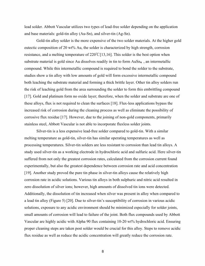
Silver-tin is a less expensive lead-free solder compared to gold-tin. With a similar
melting temperature as gold-tin, silver-tin has similar operating temperatures as well as
processing temperatures. Silver-tin solders are less resistant to corrosion than lead tin alloys. A
study used silver-tin as a working electrode in hydrochloric acid and sulfuric acid. Here silver-tin
suffered from not only the greatest corrosion rates, calculated from the corrosion current found
experimentally, but also the greatest dependence between corrosion rate and acid concentration
[19]. Another study proved the pure tin phase in silver-tin alloys cause the relatively high
corrosion rate in acidic solutions. Various tin alloys in both sulphuric and nitric acid resulted in
zero dissolution of silver ions; however, high amounts of dissolved tin ions were detected.
Additionally, the dissolution of tin increased when silver was present in alloy when compared to
a lead tin alloy (Figure 5) [20]. Due to silver-tin’s susceptibility of corrosion in various acidic
solutions, exposure to any acidic environment should be minimized especially for solder joints,
small amounts of corrosion will lead to failure of the joint. Both flux compounds used by Abbott
Vascular are highly acidic with Alpha 90 flux containing 10-20 wt% hydrochloric acid. Ensuring
proper cleaning steps are taken post solder would be crucial for this alloy. Steps to remove acidic
flux residue as well as reduce the acidic concentration will greatly reduce the corrosion rate.

9
When exposed to 3.5 wt % NaCl the opposite effect was seen, silver-tin corroded less than lead
tin [21]. Corrosion of silver-tin solder therefore is only of concern during manufacture and in
acidic environment applications, assuming proper flux removal methods are implemented.
Figure 5. The rate of Sn dissolution in 0.05 M HNO3 increases when an Sn-Ag compound is present in comparison to a Sn-Pb compound; however, the rate of pure Sn dissolution is slowed by the Sn-Ag presence [20].
1.4.3 Corrosion at Solder Joints
The typical finished guide wires contain a stainless steel core bonded to a platinum coil
with gold-tin and silver-tin solder joints. The joining of these dissimilar metals in addition to
residual flux ultimately leads to corrosion. A corrosion cell has four components: an anode, a
cathode, an electrolyte, and an electron path. In the case of galvanic corrosion, the electrode
potential between the dissimilar metals drives an ion current. At the tip of the wire, at the gold-
tin solder joint, the anode is typically the stainless steel core while the cathodes are the gold
solder and platinum coil [22]. In the situation of silver-tin solder on a stainless steel core, the
opposite is expected: the stainless steel core will become the cathode while the silver-tin solder
will become the anode (Figure 6). The electron path is the two metal electrodes since they are in
contact with one another. The electrolyte is the final component, this is fulfilled by the residual
flux residue: Zn crystals. These dehydrated crystals, which formed during the high heat of the

10
soldering process, trap any moisture from the environment. Once the crystals absorb moisture
again post processing, the electrolyte is formed and the corrosion cell complete.
The anodic regions undergo a reduction in material during corrosion; therefore, these
components are the expected sites of failure. Since neither the electrodes nor electron path can be
removed, the best form of corrosion prevention is removal of the electrolyte. This can be done by
ensuring robust cleaning steps, which prevent any residual flux residue at the solder joints.
Figure 6. The galvanic series for various metals, both 304 Stainless Steel and Gold are characterized by positive reduction potentials making them more cathodic; however, due to the difference in potentials Stainless Steel becomes the anode for the given corrosion cell [22].
Corrosion at solder joints has been studied primarily in electronics although this
corrosion ultimately caused the class I recall of guide wires in 2010. In electronic assemblies
using similar soldering operations, it was found that flux residues can promote corrosion as well
as fungus growth in humid environments [23]. Jellesen et al discuss corrosion of components and
sub-assemblies on an electronic printed circuit board assemblies (PCBAs). The study presents
the possibility of solder flux residues as corrosion promoters in a humid atmosphere [24].
Jellesen et al state that the presence of ionic substances increased the conductivity of condensed
water layers, influencing the corrosion process. Strauss also states that water-soluble (polar)
components of flux residue, in the presence of moisture, can cause electrolytic corrosion at the
interface of different metals [18]. In printed circuit boards (PCB), the behavior was observed
when moist ionic residual flux sitting on the dividing line between solder and the metallic
component of the chips formed an electrolytic cell, with a potential of 2.5 Volts. Similar
behavior was observed by Abbott Vascular and the corrosion of their guide wires in humidity.

11
The humidity resulting from packaging and handling is likely promoting corrosion with the
residual flux, as in the study discussed above.
1.4.4 Cleaning of Residual Flux
The removal of flux residue is mandatory and can be accomplished through the
utilization of elevated temperature DI water, mechanical scrubbing, or both. Abbott Vascular
uses an ultrasonic cleaner bath to remove excess flux material from soldered joints. The capacity
to effectively remove residual flux is the dependent on multiple variables, but the product design
and the type of flux used are the most important [26]. The primary requirement for the cleaning
effectiveness is good flux solvency, both fluxes used by Abbott Vascular are water-soluble
[9,10,26].
Although lead free solders are sought after for environmental and health benefits,
removal of complaint fluxes residues is more difficult. It is known that polar solvents are best for
removing polar contaminants/fluxes and that non-polar solvents are best for removal of non-
polar contaminants [26]. Yet, it is known that alcohols, polar solvents, work to remove most
contaminants and flux residues, regardless of polarity [18]. Abbott Vascular uses 100%
isopropyl alcohol in the cleaning process of their fully assembled wires.
Another requirement for effective cleaning is the water quality. Morrow discusses the
different levels of water purity as related to post-solder aqueous cleaning of soldered PCBs.
Water purity falls into three types: tap, reverse osmosis (RO), and DI water. The water’s purity is
determined by the amount of minerals and impurities present and increases from tap, to RO, and
lastly to DI water. Water impurities work to hinder the dissolving of residues/contaminants and
impede the work of detergents in aqueous-based cleaning [23]. Because of its inherent polar
nature, water does not like to be pure. The article goes on to discuss that the higher the purity, the
higher the detergent’s ability to remove impurities from the product and not from the water [23].
Abbott Vascular uses DI water for all cleaning aspects of their soldering operations. The
cleaning water temperature cannot exceed 50°C as exceedingly high temperature can results in
corrosion and/or pitting or cause secondary reactions.
Indalloy Flux #2 and Alpha Flux 90 guidelines recommend that cleaning of the solder
surfaces be performed as soon as possible after the soldering operation to prevent corrosion.

12
Indalloy Flux #2 does not progressively corrode stainless steel (no neutralization necessary), but
cleaning is still advisable as the flux/flux residue may still attack the solder [10].
2 Experimental Procedure
2.1 Safety
Safety was always made a top priority during laboratory testing. Proper personal
protective equipment (PPE) and partner system were always in effect. Additionally, lab
equipment was only used after the proper training was obtained, this included: the environmental
chamber, SEM, Mini Instron, and ultrasonic bath.
2.2 Design of Experiment To assess the effects of residual flux on guide wire integrity, an experiment was designed
utilizing two variables. The first variable considered was the amount of residual flux, using
various cleaning procedures (Table 1). The control group represents Abbott Vascular’s current
cleaning procedure during every guide wire manufacture. Both the dip in IPA and thirty second
ultrasonic bath (in DI water) are performed after each of the three solder joints are completed.
The three-minute ultrasonic bath (in DI water) is only completed once all three solder joints have
been completed. Group D represents a worst-case manufacturing condition in which ultrasonic
bath water has been contaminated while groups C and A represent the level of residual flux in
the event full cleaning is not obtained.
Table 1: Cleaning Procedures for each Level of Cleaning
Group Name Cleaning Steps Control 1. Dip in IPA post solder
2. 30 second ultrasonic bath post solder 3. 3 minute ultrasonic bath post solder
Group D 1. Dip in IPA post solder 2. 30 second ultrasonic bath post solder (bath contaminated by
residual flux) 3. 3 minute ultrasonic bath post solder (bath contaminated by
residual flux) Group C 1. Dip in IPA post solder
2. 30 second ultrasonic bath post solder Group A 1. Dip in IPA post solder

13
The second variable was extended exposure conditions. Two conditions were tested:
ambient, and extreme/elevated. Temperature and humidity were elevated simultaneously to
accelerate any effect residual flux had on the solder joints. Ambient conditions provide both a
baseline for comparison of results as well as insight to the effect of residual flux without
extended storage time contributing to reduced integrity.
Combining these two variables yielded a total of eight treatment groups (Figure 7). Each
treatment group would undergo tensile testing of every wire, followed by scanning electron
microscopy (SEM) analysis of a single wire from each group.
Figure 7. Flowchart outlining each treatment group used in the experiment. Cleaning groups ranged from least clean
to most clean from left to right.
2.3 Environmental Exposure An environmental chamber was utilized to expose specimens at 37°C and 80% RH for
two 6-hour cycles. The inside of the environmental chamber was lined with Aluminum to
minimize potential contamination of the specimens. The environmental chamber was pre-heated
before the specimens were placed inside. The specimens were placed a few centimeters apart to
ensure no contact between specimens or cross-contamination between different sample groups
(Figure 8). Each group was secured to the Aluminum lining at the proximal using masking tape.
TempTale Sensitech 4 temperature and humidity monitors were used to monitor conditions

14
throughout the exposure cycles, readings were recorded every 15 minutes. One temperature and
humidity monitor was placed near the distal end of each of the sample groups.
Figure 8. Aluminum lining of the environmental chamber. Guide wires were secured by groups and separated by
specimen. Temperature and humidity monitors (left) tracked parameters.
After each six-hour exposure, the chamber was turned off and the samples were left
inside during ramp-down of the first cycle and ramp-up of the second cycle. Nitrile gloves were
used when handling the specimens before and during exposure to minimize contamination from
oils or dirt. After exposure and before tensile testing each sample group was placed in a plastic
container for storage.
2.4 Tensile Testing A Mini Instron 55 was used to tensile test each specimen while Bluehill 3 software
plotted the stress versus percent extension outputs (Figure 9). A 500 N load cell and a 50 N load
cell were used to test the unexposed and exposed samples, respectively. A crosshead rate of 10
mm/min and a gage length of 20 cm were used. Specimens were clamped at the proximal end
using emery paper lined grips/jaws to minimize slippage. Slippage occurred during testing of
many of the specimens, but maximum peak load values were able to be obtained for all
specimens.

15
Figure 9. Mini Instron 55 tensile tester with a 500 N set-up. The proximal end of wire was clamped at
the stationary jaws, while the distal end was clamped at the moving crosshead.
The proximal end was centered on the face of the clamp by using markings of the jaws and
emery paper. The distal end was clamped using a torque device provided by Abbott Vascular
(Figure 10). The distal solder, or approximately the distal 1 mm of the wire, was inserted into the
metal jaws of the device and tightened. The torque device was then secured onto the tensile tester
using rubber grips. Both ends were clamped at the center ensure parallelism, incorrect alignment
would lead to shearing. The distal solder maximum loads were obtained for all sample groups,
despite challenges in precision required at the distal solder joint.

16
(a)
(b)
(c)
Figure 10. Wire clamping at proximal end (a) and distal solder (b). Alignment of the wire was crucial to obtain accurate results. Metal jaws of torque device (c) used to clamp solder joint.
2.5 Scanning Electron Microscopy
A FEI Quanta 200 Scanning Electron Microscope was used to characterize the fracture
surface and identify corrosion products for one wire per each treatment group. The microscope
was operated in high voltage and with an approximate working distance of 10 millimeters. Two
samples were mounted on the same stud, the ambient and elevated treatment of each cleaning
group was typically mounted together to prevent any potential for cross contamination. A spot
size of 4.0 and a voltage of 25 kV was typically used to allow for suitable resolution and focus at
higher magnification. Gloves were always used to mount samples as well as to place samples in
the SEM chamber.
2.5.1 Sample Preparation
Samples required special cleaning before being placed in the SEM. A noticeable layer of
residue could be seen on samples initially soaked in 100% IPA for three minutes. To properly
view the fracture surface and rid the samples of this residue an ultrasonic bath in 100%
anhydrous ethanol was utilized. Samples were mounted to keep the fracture surface from
touching the sides of the beaker and submerged in anhydrous ethanol. They were then placed
under ultrasonic conditions for five minutes. The samples were removed and immediately dried
with canned high-pressure air. Samples were then mounted on SEM stubs with carbon tape and
placed in a storage box.

17
3 Results
3.1 Environmental Exposure No significant differences were recorded between temperature and humidity readings
between groups in both environmental exposure cycles. However, differences in average
temperature and humidity were recorded between cycle 1 and cycle 2. Both the average
temperature and relative humidity in cycle 1 were higher than in cycle 2. During testing cycle 1,
an average of 37.23˚C during the 6-hour dwell time was recorded (Table 2). The highest average
temperature during cycle 1 was recorded for group C at 37.46˚C, while the lowest temperature
during cycle 1 was recorded for group A at 37.06˚C.
Table 2: Cycle 1 Average Dwell Time Temperature and Relative Humidity by Group.
Group(s)
Average Dwell Temperature
[℃]
Average Dwell Relative Humidity
[%] D and Control 37.18 87.448
C 37.46 86.668 A 37.06 87.692
The environmental chamber reached lower average dwell temperature and lower average
dwell relative humidity values for cycle 2 as compared to cycle 1. As outlined in Table 3, the
highest average temperature attained was recoded for sample group C, while the lowest average
dwell temperature was recorded for sample group A.
Table 3: Cycle 2 Average Dwell Time Temperature and Relative Humidity by Group.
Group(s)
Average Dwell Temperature
[℃]
Average Dwell Relative Humidity
[%] D and Control 35.28 78.318
C 35.66 79.033 A 35.20 78.610
A difference of 8.61% average dwell RH for all groups was recorded between cycle 1 and
cycle 2. Dwell RH averages for all groups for cycle 1 and cycle 2 were 87.26% and 78.65%,
respectively. Temperature and relative humidity fluctuations were experienced simultaneously

18
between groups, therefore differences in peak tensile load cannot be attributed to environmental
exposure. Appendix A displays original Temptale readings for both cycle 1 and cycle 2. 3.1.1 Environmental Exposure – Humidity
Fluctuations in % relative humidity were detected during cycle 1 (Figure 11). The
fluctuations occurred during the 6-hour dwell period but were consistent within different sample
groups.
Figure 11. Relative humidity per sample group for environmental exposure testing cycle 1. Total testing time of 8
hours; 6 hours dwell time, 1-hour ramp-up, and 1-hour ramp-down.
No major RH humidity fluctuations were recorded during dwell time for the cycle 2 of
environmental exposure (Figure 12). Fluctuations observed in cycle 1 could be attributed to
mechanical error of the chamber, given that the parameters used were near the machine’s
maximum capabilities.
82
84
86
88
90
92
94
96
0 50 100 150 200 250 300 350 400 450 500
Rel
ativ
e Hum
idity
[%]
Time [min]
100% Clean 50% Clean 0% Clean

19
Figure 12. Relative humidity per sample group for environmental exposure testing cycle 2. Total testing time of 8
hours; 6 hours dwell time, 1-hour ramp-up, and 1-hour ramp-down.
3.1.2 Environmental Exposure – Temperature
Temperature fluctuations during the 6-hour dwell were recorded during the
environmental exposure cycle 1 (Figure 13). The fluctuations occurred simultaneously at 165
min and 360 min between temperature and humidity and were constant between different sample
groups. The lowest temperature recorded for all groups during cycle 1 as a result of fluctuation
was 36.66 ℃. The highest temperature fluctuation was recorded at 37.61℃.
35404550556065707580859095
100
0 40 80 120 160 200 240 280 320 360 400 440 480
Rel
ativ
e Hum
idity
[%]
Time [mm]
Group D and Control Group C Group A

20
Figure 13. Temperature per sample group for environmental exposure testing cycle 1. Total testing time of 8
hours; 6 hours dwell time, 1-hour ramp-up, and 1-hour ramp-down.
No fluctuations in temperature were recorded during enviromental exposure cycle 2 (Figure
14). The lack of fluctiation during the 6-hour dwell could be credited to the lower average
temperatures recorded as the machine did not run near it maximum cpacity. The highest and lowest
fluctuations recorded deviated by 1.64% and 0.92% from the target temperature, respectively.
Therefore, temperature fluctuations did not influence differences between sample groups.
Figure 14. Temperature per sample group for environmental exposure testing cycle 2. Total testing time of 8
hours; 6 hours dwell time, 1-hour ramp-up, and 1-hour ramp-down.
90
92
94
96
98
100
102
0 50 100 150 200 250 300 350 400 450 500
Tem
pera
ture
[F]
Time [min]
Group D and Control Group C Group A
0
20
40
60
80
100
120
0 40 80 120 160 200 240 280 320 360 400 440 480
Tem
pera
ture
[F]
Time [min]
Group D and Control Group C Group A

21
3.2 Tensile Testing Tensile testing yielded results with little variation relative to the maximum loads, and few
outliers were seen in the elevated exposure groups (Figure 15). This suggests the test setup
allowed for accurate and reproducible results. Treatments undergoing elevated exposure each
contained eight specimens and appeared to be normally distributed. Ambient exposure groups
contained two to four specimens and in return did not exhibit normal distributions for each
treatment. Differences in sample size are attributed to availability; however, it was ensured that
all exposed sample groups had a constant sample size of 8. A 500 N load cell was used to test all
ambient exposed samples, and a 50 N load cell was used to test the elevated exposure treatments.
This was due to an intradepartmental move of the Mini Instron, and may be a factor in the
magnitude of load decrease between ambient and elevated treatments. This however could not be
verified with the testing done; therefore, data will be analyzed as it was received. No difference
from testing method and procedures will affect the data from cleaning groups undergoing the
same exposure. These comparisons within exposure type will be the most useful in analyzing the
effect of varying residual flux on guide wires.
Figure 15. Box plots for maximum load data (N) from distal solder joint tensile testing of each treatment group.

22
3.2.1 Group A
Group A averaged maximum loads of 19.52 N and 13.43 N for ambient and elevated
exposures, respectively (Figures 16 and 17). Elevated exposure specimens likely experienced
more noise in each curve due to the use of a more sensitive load cell.
Figure 16. Load [N] versus tensile strain [%] (extension) for ambient exposure group A samples.
Figure 17. Load [N] versus tensile strain [%] (extension) for elevated exposure group A samples.
The displacement of group A accelerated exposure specimen 8 curve is due to failure in zeroing extension during test set-up (Figure 17).
02.5
57.510
12.515
17.520
22.5
0 0.2 0.4 0.6 0.8 1 1.2 1.4 1.6 1.8
Load
[N]
Tensile Strain [%]Specimen 1 Specimen 2 Specimen 3

23
3.2.2 Group C
Group C averaged maximum loads of 20.1 N and 13.91 N for ambient exposure and
elevated exposure, respectively (Figures 18 and 19). Fluctuations in load values during testing
are a result of slipping of the 304 SS coil at the proximal end.
Figure 18. Load [N] versus tensile strain [%] (extension) for ambient exposure group C samples.
Figure 19. Load [N] versus tensile strain [%] (extension) for elevated exposure group C samples.
3.2.3 Group D
Group D averaged maximum loads of 21.34 N and 13.29 N for ambient exposed samples
and elevated exposed samples, respectively (Figures 20 and 21). Group D obtained higher peak
loads than groups A and C in both exposure conditions.

24
Figure 20. Load versus tensile strain [%] outputs for group D* exposed to ambient conditions. * specimens were
handled with contaminated gloves and subject to water containing acidic flux.
Figure 21. Load versus Load versus tensile strain [%] outputs for group D* exposed to elevated conditions. *
specimens were handled with contaminated gloves and subject to water containing acidic flux
3.3.3 Control
Control group specimens achieved some of the highest loads with respect to other
treatments of the same exposure. Loads averaged 23.83 N and 15.31 N for ambient and elevated
exposures respectively (Figures 22 and 23). Elevated exposure specimens experienced noticeably
greater amount of slip during testing.

25
Figure 22. Load versus tensile strain [%] outputs for control specimens exposed to ambient conditions.
Figure 23. Load versus tensile strain [%] outputs for control specimens exposed to elevated conditions.
Samples experiencing the most slippage were randomly distributed throughout the order
of samples tested; therefore, wear on the torque device was not the cause (Figure 24). The slip
was suspected to take place in the lower grips since each wire was placed in a slightly different
position on the emery paper. Once the emery paper was replaced, future specimens no longer
experienced the high level of slip as seen in the elevated exposure control group; therefore, slip
at the proximal end was the likely cause and does not affect the maximum load measurement of
this treatment group.

26
Figure 24. Specimens with increased slippage shown with increased transparency to reduce clutter in chart.
3.4 Scanning Electron Microscopy
SEM analysis on each treatment group presented some challenges due to the high
magnification required to properly analyze the modes of fracture on each specimen. Overall
images of each sample were taken as approximately 2200x. Ultrasonic cleaning of each control
treatment allowed for proper fracture mode characterization of each area along the fracture
surface.
3.4.1 Group A
Both types of exposure for group A specimens exhibited dramatically different fracture
surfaces in relation to every other treatment group (Figure 25). A noticeable amount of surface
contamination is seen on both specimens, in the form of charging particles as well as surface
residue. Once an additional group A elevated exposed specimen was ultrasonically cleaned, a
cup and cone fracture was visible (Figure 26).

27
(a) (b)
Figure 25. Group A ambient (a) and elevated exposure (b).
(a) (b)
Figure 26. Elevated exposure, group A specimen after ultrasonic cleaning. An overall cup and cone fracture surface (a) with a clear interface between low energy ductility and high energy microvoid coalescence (b).
3.4.2 Group C
Each specimen in the two group C treatments is characterized by areas of high energy
ductile fracture, and larger areas of extremely low ductility (Figure 27). Neither sample
displayed signs of microscale brittleness. Although the ambient exposed sample contained a
large crack running towards the inclusion in the bulk material, the sample had a significantly

28
greater maximum load (Figure 28). This suggests small characteristics in the elevated exposure
treatments led to a deterioration in strength.
(a) (b)
Figure 27. Group C ambient (left) and elevated (right) exposure specimens.
Figure 28. Group C ambient exposure displaying mixed modes of fracture.
3.4.3 Group D
As a higher level of cleaning is achieved, ambient and elevated exposure treatments
display smaller differences. Both specimens display areas of high and low energy ductile
fracture; however, ambient exposures still appear to contain higher degrees of microvoid
coalescence in comparison to their elevated exposure treatments (Figures 29 and 30).

29
(a) (a) (b)
Figure 29. Group D specimens from ambient (left) and elevated (right) exposure treatments.
Figure 30. Ambient exposed group D specimen at a higher magnification to show high and lower energy ductile
fracture surfaces.
3.4.4 Control
Each sample contains a slight cup and cone fracture surface, but the elevated exposure
sample contains greater amounts of surface flaws along the side of the wire (Figure 31). This
may be a sign on corrosion along the outer surface of the wire. Further testing on more
specimens would be required to verify this.

30
Figure 31. Control specimens from ambient (left) and elevated (right) exposure treatments.
4 Analysis
A noticeable drop was seen between ambient and elevated exposure groups, and this was
supported by a statistically significant difference, at 𝛼=0.05, in ANOVA post-hoc analysis
(Table 4). ANOVA analysis revealed a statistical difference between one or more treatments;
therefore, a student’s t test was run on each variable and the cross of the two. An 𝛼=0.05 was
used for each of the post-hoc tests (Appendix B). Fewer statistical differences were seen between
different cleaning groups with the same exposure. Ambient exposed treatments only contained a
significant difference between control and cleaning groups C and A. This may be due to the
small sample size producing high amounts of uncertainty in the true data spread for each
treatment. Group D connected the control and other cleaning groups, being statistically different
from neither. Elevated exposure treatments exhibited clearer results with the control group being
the only significantly different group. Little variation in temperature and humidity during both
exposure cycles was seen between each group; therefore, varying exposure is not a confounding
variable between these cleaning groups.

31
Table 4: Student’s t Test Results as calculated with JMP software.
Level Least Squares Mean
Ambient, Control A 23.825
Ambient, Group D A B 21.345
Ambient, Group C B 20.100
Ambient, Group A B 19.520
Elevated, Control C 15.471
Elevated, Group C D 13.944
Elevated, Group A D 13.430
Elevated, Group D D 13.025
Levels not connected by the same letter are significantly different.
SEM analysis provided some insight to the drop in maximum loads under certain
treatments. No explicit signs of corrosion or pitting could be seen along the fracture surface
likely due to the extremely small area in addition to the relatively short amount of time
specimens spent at elevated temperature and humidity. The main mode of fracture for every
treatment group appeared to be ductile cup and cone in nature. Group A was the only group to
exhibit a drastically different mode of fracture. In comparing the amount of microvoid
coalescence on each surface, lower levels of cleaning were seen to contain both less area as well
as lower energy forms of microvoid coalescence. This indicates that an increased amount of
residual flux reduces the ductility of each specimen. This is also seen in the lower extensions
during tensile testing. At the small scale of the fracture surface, any level of decreased
microscopic ductility, will cause the specimen to exhibit brittle fracture characteristics
macroscopically.
5 Conclusions 1. Extreme exposure of medical guide wires in elevated temperature and humidity leads to
degradation of peak tensile loads for distal tip soldered joints.
2. Any level of residual acidic soldering flux results in diminished peak loads, despite ambient
or extreme conditions.
3. Lower levels of microscopically ductile fracture led to macroscopically brittle fracture and
lower loads in elevated exposure treatment of guide wires also exposed to residual flux.

32
6 References [1] Abbott Laboratories. (2019). Retrieved from
https://en.wikipedia.org/wiki/Abbott_Laboratories
[2] Company Overview of Abbott Vascular Inc. (2019). Retrieved from
https://www.bloomberg.com/research/stocks/private/snapshot.asp?privcapId=33102937
[3] Abbott Cardiovascular | Life-Changing Technology Keeping Hearts Healthy. (2019).
Retrieved from https://www.cardiovascular.abbott/us/en/home.html
[4] Abbott Inc. (2018, April 18). Xience: Patient Information Guide [Everolimus Eluting
Coronary Stent System].
[5] Fornell, D. (2019). Understanding the Design and Function of Guide wire Technology.
Retrieved from https://www.dicardiology.com/article/understanding-design-and-function-guide
wire-technology
[6] Lanzer, P. (2018). Textbook of Catheter-Based Cardiovascular Interventions, (Second Edition).
https://doi.org/10.1007/978-3-319-55994
[7] Barik, R. (2019). Coronary Guide wires: Choice and Appropriate Use in PCI. Presentation.
[8] TurnTrac Guide wire Packaging (2019), Abbott Vascular Inc.
[9] Cookson Electronics, “Material Safety Data Sheet: Alpha 90 IA Flux”, 3 February 2009.
[10] Indium Corporation of America, “Safety Data Sheet: Indalloy Flux 2”. SDS- LF002. 7
November 2016.
[11] “MAUDE Adverse Event Report: BOSTON SCIENTIFIC - MAPLE GROVE KINETIX
PTCA GUIDE WIRE WIRE, GUIDE, CATHETER.” Accessdata.fda.gov, FDA,
www.accessdata.fda.gov/scripts/cdrh/cfdocs/cfmaude/detail.cfm?mdrfoi__id=1842547.
[12] Alloy Temperature Chart. Kester,
www.kester.com/Portals/0/Documents/Knowledge20Base/Alloy%20Temperature%20Chart.pdf.
[13] Anhock, S., et al. “Investigations of Au-Sn Alloys on Different End-Metallizations for High
Temperature Applications [Solders].” Twenty Second IEEE/CPMT International Electronics
Manufacturing Technology Symposium. IEMT-Europe 1998. Electronics Manufacturing and

33
Development for Automotives (Cat. No.98CH36204), Apr. 1988,
doi:10.1109/iemte.1998.723081.
[14] “Effective Date of Lead Ban.” Received by Betsy Devlin, EPA, 1988.
[15] Shefa, Syeda T., and Paul Héroux. “Both Physiology and Epidemiology Support Zero
Tolerable Blood Lead Levels.” Toxicology Letters, vol. 280, 2017, pp. 232–237.,
doi:10.1016/j.toxlet.2017.08.015.
[16] “Gold/Tin Solder Alloy: Applications & Alloy Composition Choices.” Indium Corporation,
www.indium.com/blog/goldtin-applications-and-alloy-composition-choices.php.
[17] Jacobson, David M., and Giles Humpston. “Gold Coatings for Fluxless Soldering.” Gold
Bulletin, vol. 22, no. 1, 1989, pp. 9–18., doi:10.1007/bf03214704.
[18] Strauss, Rudolf, and Rudolf Strauss. SMT Soldering Handbook. 2nd ed., Newnes, 2001, pp.
261-323.
[19] Vani, R., et al. “Comparative Study on Corrosion of SN-3.5AG and SN-9ZN Solders in
Acidic Environment.” National Conference on Challenges in Research & Technology in the
Coming Decades (CRT 2013), 2013, doi:10.1049/cp.2013.2559.
[20] Mori, Masato, et al. “Corrosion of Tin Alloys in Sulfuric and Nitric Acids.” NeuroImage,
Academic Press, 5 Dec. 2001, www.sciencedirect.com/science/article/pii/S0010938X01000944.
[21] Li, Dezhi, et al. “Corrosion Characterization of Tin–Lead and Lead Free Solders in 3.5wt.%
NaCl Solution.” Corrosion Science, vol. 50, no. 4, 2008, pp. 995–1004.,
doi:10.1016/j.corsci.2007.11.025.
[22] Jenks, R. (2019). Section 4 - The Book of Metal. Retrieved from
https://www.slackademics.com/boltingbibleblog/section3-metal
[23] Morrow, D. “Don’t Drink the Water Cleaner PCBs can mean less assembly failures”.
Printed Circuit Fabrication. 1999, pp. 50-51.
[24] Jellesen, Morten S., et al. “Corrosion Failure Due to Flux Residues in an Electronic Add-on
Device.” Engineering Failure Analysis, vol. 17, no. 6, 2010, pp. 1263–1272.,
doi:10.1016/j.engfailanal.2010.02.010.

34
[25] Ultrasonic cleaning. (2019). Retrieved from
https://en.wikipedia.org/wiki/Ultrasonic_cleaning
[26] Willis, B. (2003). Reflow Soldering Processes and Troubleshooting SMT, BGA, CSP and
Flip Chip Technologies, 15(1). https://doi.org/10.1108/ssmt.2003.21915aae.003

I
7 Appendix Appendix A: Original Temptale Data for the Full Elevated Exposure Run
Figure 1. Original group A Temptale data for both exposure cycles as well as ramp up and ramp down times.
Figure 2. Original group C Temptale data for both exposure cycles as well as ramp up and ramp down times.

II
Figure 3. Original group D and control Temptale data for both exposure cycles as well as ramp up and ramp down times.

III
Appendix B: ANOVA and Post-Hoc Analysis