Jurnal Kejuruteraan 23(2011): 57-68

Effect of Soil Porosity and Slope Gradient on the Stability of Weathered Granitic Hillslope

(Kesan Keliangan Tanah dan Kecerunan Cerun pada Kestabilan Cerun Bukit Granit Terluluhawa)

Muhammad Mukhlisin & Mohd Raihan Taha

ABSTRACT

Modeling rainwater infiltration in slopes is vital to the analysis of rainfall induced slope failure. Amongst the soil hydraulic properties, the hydraulic conductivity K and considered as the most dominant factor affecting the slope stability. Of less prominent was the effect of water retention characteristics. In this study, a numerical model was developed to estimate the extent of rainwater infiltration into an unsaturated slope, the formation of a saturated zone, and the change in slope stability. This model is then used to analyze the effects of the soil porosity parameters (i.e., saturated soil water content qs and effective soil porosity (ESP)) and slope gradient on the occurrence of slope failure. Results showed that when the surface soil of a slope has a relatively large ESP value, it has a greater capacity for holding rainwater, and therefore delays rainwater infiltration into the subsurface layer. Consequently, the increase in pore water pressure in the subsurface layer is also delayed. In this manner, a relatively large surface layer ESP value contributes to delaying slope failure. In addition, the slope gradient of slope is also a significant parameter in slope stability analysis. The time taken for gentle slope to reach failure is longer compared to similar cases with 40o slope gradient.

Keywords: Effective soil porosity; slope gradient; slope stability; granite soil

ABSTRAK

Pemodelan penyusupan air hujan dalam cerun adalah penting untuk analisis hujan yang menyebabkan kegagalan cerun. Antara ciri-ciri hidraulik tanah, konduktiviti hidraulik K dianggap sebagai faktor yang paling dominan yang mempengaruhi kestabilan cerun. Ciri yang kurang penting adalah kesan ciri-ciri pengekalan air. Dalam kajian ini, model berangka telah dibangunkan untuk mengira sejauh manakah penyusupan air hujan ke dalam cerun tidak tepu, pembentukan zon tepu, dan perubahan dalam kestabilan cerun. Model ini kemudiannya digunakan untuk menganalisis kesan parameter keliangan tanah (iaitu kandungan air tanah tepu qs dan keliangan berkesan tanah (ESP)) dan kecerunan apabila berlaku kegagalan cerun. Hasilnya menunjukkan bahawa apabila tanah permukaan cerun mempunyai nilai ESP yang agak besar, ia mempunyai kapasiti yang lebih besar untuk memegang air hujan, dan oleh itu menunda penyusupan air hujan ke dalam lapisan bawah permukaan. Oleh itu, kenaikan tekanan air liang di lapisan bawah permukaan juga ditangguhkan. Dengan cara ini, nilai ESP yang agak besar bagi lapisan permukaan menyumbang kepada melambatkan kegagalan cerun. Di samping itu, kecerunan cerun juga merupakan parameter penting dalam analisis kestabilan cerun. Masa yang diambil untuk cerun yang landai untuk mencapai kegagalan adalah lebih lama berbanding dengan kes-kes yang serupa dengan kecerunan cerun 40o.

Kata kunci: Keliangan berkesan tanah; kecerunan cerun; kestabilan cerun; tanah granit

INTRODUCTION

Modeling rainwater infiltration in slopes is vital to the analysis of slope failure induced by heavy rainfall. Numerical models have been used previously by Tsaparas et al. (2002), Cho and Lee (2001), Gasmo et al. (2000), Wilkinson et al. (2002), Mukhlisin et al. (2006), Gofar and Lee (2008) to study the effect on slope stability of rainwater infiltration into unsaturated soils. In order analyze rainwater infiltration into soil, it is important to have an understanding of the hydraulic properties of the soil, in

particular the relationship between volumetric water content θ (cm3 cm-3) and soil capillary pressure ψ (cm), and the relationship between unsaturated hydraulic conductivity K (cm s-1), and ψ. These relationships are known as the water retention curve and the hydraulic conductivity function, respectively.

Among soil hydraulic properties, the hydraulic conductivity K, a measure of the ability for water movement in soil, has been frequently analyzed for its effects on slope stability. Previous studies (e.g., Reid

58

1997; Cai et al. 1998; Cho and Lee 2001) reported that variation in hydraulic conductivity K, can modify pore water pressure distribution, and therefore the effective stress of soil and slope stability during rainfall infiltration. Reid (1997) examined the destabilizing effects of small variations in hydraulic conductivity by using ground-water flow modeling, finite-element deformation analysis, and limit-equilibrium analysis. The author concluded that earth materials with similar textures can have hydraulic conductivity variations of several orders of magnitude and frictional strength variations of about 4-8o. The destabilizing pore pressure effects induced by small hydraulic conductivity variations can be as great as those induced by these frictional strength variations. Cai et al. (1998) reported the effects of horizontal drains on ground water levels during rainfall by applying three-dimensional finite element analysis of transient water flow through unsaturated to saturated soils. The authors concluded that the effects of horizontal drains are mainly dependent on the ratio of rainfall intensity to saturated hydraulic conductivity. In another study, Cho and Lee (2001) used numerical methods to examine the mechanisms of slope failure within a soil mass during rainfall infiltration. The authors concluded that the stress field, which is closely related to slope stability, is modified by pore water pressure distribution, which is controlled by the spatial variation of hydraulic conductivity during rainfall infiltration. In addition, Reid et al. (1998) demonstrated that a small down slope decrease in soil hydraulic conductivity can decide the location of a landslide. In contrast, few studies have been published on the effects of water retention characteristics (i.e., the relationship between volumetric water content θ and soil capillary pressure ψ) on slope stability.

The water retention curve is considered one of the most fundamentally important hydraulic characteristics of soil (Assouline and Tessier 1998). On the water retention curve, the volumetric water content θ is equal to the saturated water content θs (cm3 cm-3) when the soil capillary pressure ψ is equal to zero. As ψ decreases below zero, θ usually decreases according to an S-shaped curve with an inflection point. As ψ decreases further, θ decreases seemingly asymptotically toward a soil-specific minimum water content known as the residual water content θr (cm3 cm-3). As a result, most retention models (e.g., Brooks and Corey 1964; van Genuchten 1980; Kosugi 1994) described retention curves in the range of θr ≤ θ ≤ θs. The difference between θs and θr is the effective soil porosity (ESP), and represents the total volume of drainable soil pores per unit volume of soil. Hence, ESP is directly related to the water-holding capacity of a soil and can be a dominant parameter in the characterization of rainwater infiltration and the occurrence of slope failure. Moreover, each of the soil porosity parameters exerts some control over a slope’s soil moisture conditions, and therefore determines the water content of the disturbed material which is one of key factors controlling the mobility of rainfall-induced landslides.

In this study, numerical models are developed to estimate the extent of rainwater infiltration into an

unsaturated slope, the formation of a saturated zone, the change in slope stability. This model is then used to analyze the effects of the soil porosity parameters and slope gradient on the occurrence of slope failure.

NUMERICAL STUDY

INFILTRATION ANALYSIS

TWO-DIMENSIONAL UNSATURATED FLOW EQUATION FOR SOIL WATER

According to the Darcy-Buckingham equation, horizontal and vertical water flux (qx and qz) in unsaturated soil are expressed as follows:

∂∂

+∂

∂−=

∂∂

zq

xq

tzxθ

( ) ( ) ( ) ( )ψψψψψψψ Kzz

Kzx

Kxt

C∂∂

+

∂∂

∂∂

+

∂∂

∂∂

=∂

∂

where K(ψ) is the hydraulic conductivity as a function of capillary pressure ψ. The equation for continuity of water is expressed as

(1)

(2)

(3)

(4)

(5)

(6)

where t is time. Substituting Eq. (1) and Eq. (2) into Eq. (3) yields the two-dimensional, vertical and horizontal flow equation for soil water (Richard’s Equation):

where (cm-1) is the water capacity function defined as the slope of the soil water retention curve. Solving Eq. [4] requires the use of models for soil water retention and hydraulic conductivity.

MODEL FOR SOIL HYDRAULIC PROPERTIES

The Lognormal (LN) model proposed by Kosugi (1996, 1999), which was developed by assuming a lognormal soil-pore size distribution, is used to solve Eq. [4]. Based on the LN model, the effective saturation Se(ψ) and the water capacity C(ψ) are expressed as follows:

( ) ψθψ ddC /=

59

(7)

(8)

(9)

where θs and θr are the saturated and residual water contents, respectively, σ is a dimensionless parameter, ψm is the capillary pressure head related to median pore radius (cm), and Q denotes the complementary normal distribution function defined as

The expression of K with respect to Se and with respect to ψ are (Kosugi 1999)

where Ks is the saturated hydraulic conductivity, and α and β are dimensionless parameters that are used to characterize soil pore tortuosity. Applying the LN model, soil hydraulic properties are characterized by the seven parameters θs, θr, ψm, σ, Ks, α, and β.

SOIL HYDRAULIC PARAMETERS

Granite soils are known to be very sensitive to weathering and vulnerable to landslides. In Japan, many disasters have occurred in granite soil areas following heavy rains, resulting in a total of more than 1000 casualties over the last 62 years. In all of these cases, the major disasters resulting from these rainstorms were owing to landslides that occurred on weathered granite slopes (Chigira 1999). Therefore, this study analyzed rainwater infiltration and slope stability by assuming weathered granite soil properties.

A number of data sets on the hydraulic properties of weathered granite soils were collected from published (Ohta et al. 1985; Shinomiya et al. 1998; Hendrayanto et al. 1999) and unpublished studies (Shinomiya and Kosugi, personal communications). These data sets include the observed values of saturated and unsaturated hydraulic conductivities, saturated water contents, and retention curves.

Observations were divided into surface and subsurface soil layers, and comprised two sample sets of 34 and 18 samples of soil that were taken from 5- to 25-cm depths and from 70- to 170-cm depths, respectively.

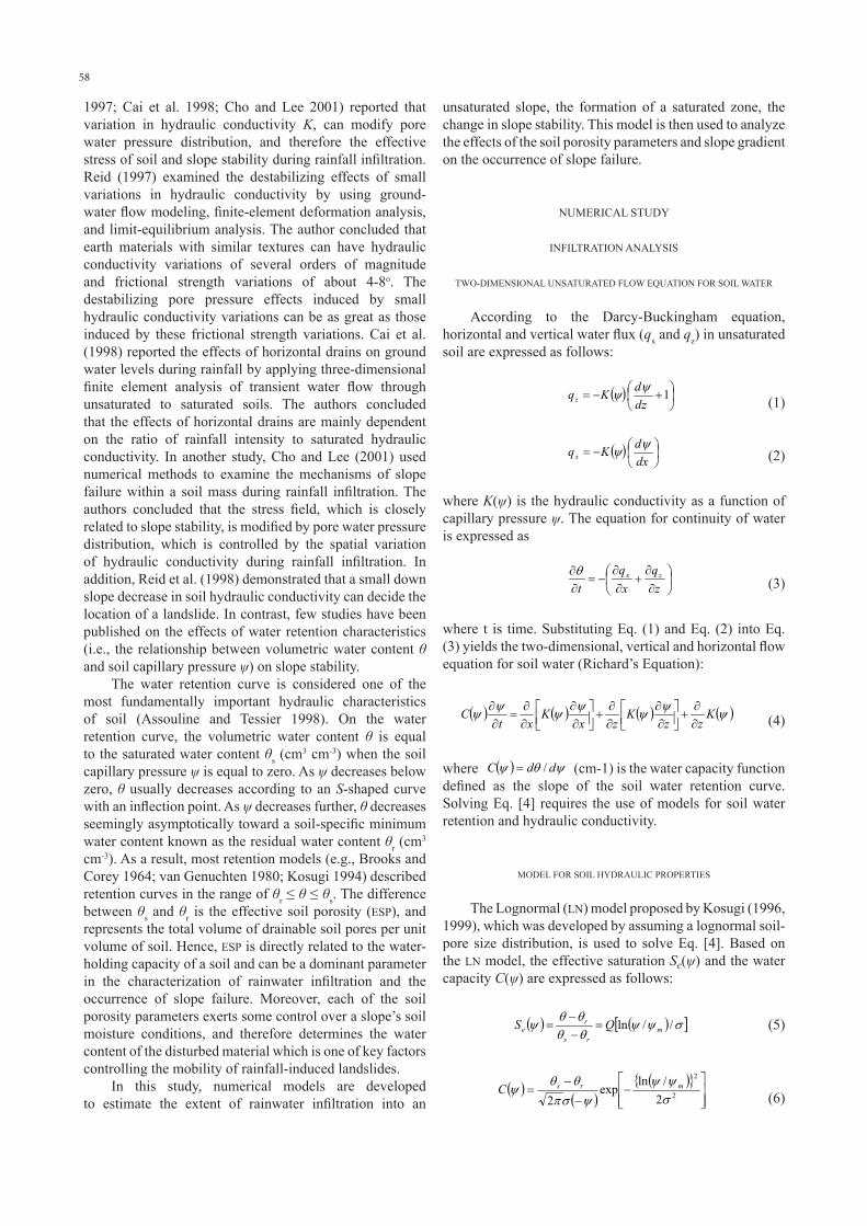
Figures 1a and b show the water capacity function (i.e., C(ψ) curve) of the surface and subsurface soils, derived by numerically differentiating the observed retention data. The figures show that the surface soil layer has greater average C(ψ) values than those of the subsurface soil layer in the range of |ψ| < 20 cm. The LN model expressed as Eq. [6] was fitted to the average curve of the observed data. When the model was applied, the θs value was fixed at the observed average value shown in Table 1. The optimized parameter values are summarized in Table 1. It is evident that the surface soil has a larger ESP (= θs-θr) value than the subsurface soil, which indicates the greater water-holding capacity of the surface soil. Figure 1 shows that Eq. [6] successfully describes the average C(ψ) curves.

Figures 2a and b show the observed K-ψ curves of the surface and subsurface soils. The figures show that the surface soil has greater average K values than the subsurface soil near saturation. However, in the dry region (|ψ| > 100 cm), the surface soil has smaller K values than the subsurface soil. The LN model expressed as Eq. [9] was fitted to the average curve of the observed data. When the model was applied, the Ks value was fixed at the observed average value shown in Table 1. The optimized parameter values (i.e.,α and β) are summarized in Table 1. Equation [9] successfully reproduces the average K-ψ curves for both the surface and subsurface soils.

Layer Datanumber θs θr θs-θr

ψm σ Ks α β

cm cm/sSurface 34 0.621 0.370 0.251 -14.3 0.92 0.0322 -0.747 2.899

Sub-surface 18 0.456 0.242 0.214 -33.8 0.98 0.0079 -1.258 2.964

TABLE 1. Fitted parameters of the Lognormal (LN) model for weathered granite forest soils†

† θs, saturated water content; θr , residual water content; ESP, effective soil porosity; ψm and σ, parameters in the retention and conductivity models expressed as Eq. [5] through [9]; Ks, saturated hydraulic conductivity; α and β, parameters in the conductivity model expressed as Eq. [8] and [9].

SOIL POROSITY

The effects of soil porosity were examined by assuming three different cases of ESP values (Cases 1 through 3) for the surface and subsurface layers. Among these cases, observed ESP values were used for case 2.

Compared with case 2, the ESP value was decreased

by 50% for case 1 by decreasing the θs value while the θr value was fixed at the same value as in case 2. Compared with case 2, the ESP value was increased by 50% for case 3 by increasing the θs value, while the θr value was fixed at the same value as in case 2 (see Figure 1). Variation among cases 1 through 3 was aimed at examining the effects of

60

soil structure development on rainwater infiltration and slope stability, since the θs value of forest soil is expected to increase as the secondary pores are formed by forest ecosystem (plant and animal) activities. Figure 1 shows that, if the ESP value is decreased or increased by 50%, the

FIGURE 1. Observed, averaged, and fitted C(ψ) curves for (a) the surface and (b) subsurface soils. The fitted curve was used for case 2. The dotted line represents the C(ψ) curve when the average (θs-θr) value is decreased by 50% (used for case 1). The thick line represents the C(ψ) curve when the average (θs-θr) value is increased by 50% (used for case 3).

FIGURE 2. Observed, averaged, and fitted hydraulic conductivity curves for (a) the surface and (b) subsurface soils.

Layer Case 1 2 3 1’ 3’ 2a 2b

Surface θs 0.495 0.621 0.747 0.621 0.621 0.747 0.495

θr 0.370 0.370 0.370 0.495 0.244 0.495 0.244

θs-θr 0.125 0.251 0.377 0.126 0.377 0.252 0.252

TABLE 2. The value of θs, θr, and (θs-θr) for the surface layer assumed for the seven simulation cases

|ψ| (cm)1 10 100 1000

C(ψ

) (cm

-1)

0.000

0.005

0.010

0.015

0.020

0.025

observedaveragedcase 2case 3case 1

|ψ| (cm)1 10 100 1000

observedaveragedcase 2case 3case 1

(a) (b)

|ψ| (cm)

0 50 100 150 200 250

K observedK averagedK fitted

|ψ| (cm)

0 50 100 150 200 250

K (c

m/s)

-9

-8

-7

-6

-5

-4

-3

-2

-1

0K observedK averagedK fitted

(a) (b)

resulting C(ψ) functions are still within the range in which the observed data exist. Since it was found that there was no clear relationship between the observed Ks and θs among surface or subsurface soils, Ks value was always fixed at the observed average values as summarized in Table 1.

The parameters used in case 2 correspond to the average observed values summarized in Table 1.

61

FIGURE 3. Curves for ( )ψC and ψθ −

FIGURE 4. θ - ψ curve with ESP (θs-θr) variation, (a) variable θs and fixed θr, (b) fixed θs and variable θr,(c) variable θs and variable θr

ψ

θ or ( )ψC

sθ

rθ

rs θθ −

( )ψC curve

ψθ − curve

θ

θs

θr 2

ψ

θr θr

θs θs

θ θ

1

2

3

2

3’

2a

2b

1’

(a) (b) (c)

ψ ψ

Figure 3 illustrates the relationship between the θ - ψ curve and the water capacity function C(ψ). The C(ψ) function is derived by differentiating the θ - ψ curve. On the θ - ψ curve, θ changes are in the range of θr ≤ θ ≤ θs. Therefore, the whole area surrounded by the C(ψ) function and the x-axis should be equal to the effective porosity (θs-θr).

FIGURE 5. Geometry of the slope used for numerical analysis (standard case with a soil depth of 100 cm and slope gradient of 40o).

The effects of soil porosity were examined by assuming seven different cases of θs, θr, and (θs-θr) values for the surface layer as summarized in Table 2. The changes in θ- ψ curve resulting from these seven different combinations are illustrated in Figure 4. In Table 2 and Figure 4, case 2 corresponds to the average observed retention curve expressed by the parameters summarized in Table 1 and 2.

In addition to cases 1 through 3, four additional cases (i.e., cases 1’, 3’, 2a, and 2b in Table 2 and Figure 4) were analyzed to clarify the effects of the soil porosity parameters (i.e., θs, θr, and (θs-θr)) on rainwater infiltration and slope stability. For case 1’, the (θs-θr) value was decreased by 50% compared with case 2 by increasing the θr value, while the θs value was fixed at the same value as case 2 (Figure 4b). Compared with case 2, the (θs-θr) value was increased by 50% for case 3’ by decreasing the θr value (Figure 4b). Both cases 2a and 2b have the same (θs-θr) value as case 2, although case 2a has greater θs and θr values than case 2, and case 2b has smaller θs and θr values than case 2 (Figure 4c).

GEOMETRY AND BOUNDARY CONDITIONS

The standard slope assumed for the numerical simulation had two soil layers (i.e., the surface and subsurface layers) with a length of 20 m and a 40o slope gradient (Figure 5). Total soil depth was 100 cm, and it was assumed that the depths of surface and subsurface soil for each layer were the same. This depth is typical of many of the granite areas (ranging between 50 and 300 cm) where landslides occurred in Japan (e.g., Shimizu et al. 2002).

Assuming an impermeable bedrock layer under the subsurface soil layer, a no-flux boundary condition was applied to the bottom of the soil layer. A no-flux condition was also applied to the top slope (a dividing ridge) and bottom slope (hollow) boundaries. Rainwater was applied to the soil surface, and when the soil surface was saturated, discharge from that section was computed. That is, the seepage face boundary condition was applied to the soil surface. Richards Equation (Eq. [4]) was numerically solved by using the finite element method (Istok 1989). The discretizing system are shown in Figure 5. As shown in the figure, triangular elements were used.

100 cm

2000

cm

40o

Bedrock

Surface

layer

Sub-surfa

ce lay

er

Point o

f the p

ressure

obser

vation

C(ψ) curve

θ - ψ curveθ or C(ψ)

θ

θs

θr

θ

θs

θr

θ

θs

θr

62

HYETOGRAPH AND INITIAL CONDITIONS

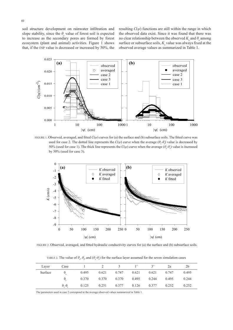
On July 20, 2003, localized torrential rainfall in the mid-southern region of Kyushu in Japan triggered a large-scale debris flow along the Atsumari-gawa River in Hougawachi, Kumamoto Prefecture. Ten houses were destroyed instantly and nineteen people were killed. The volume of sediment discharge was estimated at about 100,000 cubic meters, making this one of the largest debris flows in recent years. This study used the Hougawachi rainstorm as the input data for a hyetograph. The total rainfall, peak rate, and event duration were established at 379 mm, 91 mm/h, and 10 h, respectively.

To establish the initial conditions for the numerical simulations, a 50%-reduced hyetograph of the Hougawachi rainstorm (the total rainfall, peak rate, and event duration of this hyetograph were 189.5 mm, 45.5 mm/h, and 10 h, respectively) was initially applied. Next, a drainage duration of 48 h was simulated for the standard case of the simulation, and the resulting capillary pressure distribution within the whole slope was used for the initial condition for the main simulation.

It was assumed that the whole slope had a constant capillary pressure value, ψini, just before the 50%-reduced hyetograph was applied. The value of ψini was fixed at -100 cm. The ψini values of -50 and -200 cm were also tested, and it was found that the ψini value did not cause significant differences in the capillary pressure distribution within the whole slope at the end of the 48-h drainage.

SCENARIOS FOR NUMERICAL SIMULATION

Two scenarios were used for numerical simulation, summarized in Table 2. The first scenario (scenario 1) used the standard conditions discussed previously. That is, a drainage period of 48 h, a soil thickness of 100 cm, and a slope gradient of 40o were assumed. The soil porosity parameters were changed only for the surface layer, as in the seven cases summarized in Table 2 and Figure 4. For the subsurface layer, the soil porosity value was fixed at the same value as case 2.

In scenario 2, the slope gradient was changed from 40o to 35o, while the other parameters remained the same as in scenario 1. The seven cases of soil porosity parameter sets were examined by changing the retention curves of the surface layer.

SLOPE STABILITY ANALYSIS

Following Sammori (1994), the Bishop method (Bishop 1954) was used in conducting the slope stability analysis. In this method, the safety factor (Fs) is computed based on the moment equilibrium among slices in a sliding circle:

( )∑∑ =

=

+

−+=

I

i iii

iiiiiiI

iii

FsGuWGc

WFs

1

1

/tansincostan

sin

1φδδ

φ

δ(10)

where I is the total number of slices in the sliding circle, ui (cm) is the positive pore water pressure at the bottom of the slice i, Wi (g) is the weight of the slice i, Gi (cm) is the horizontal length of the slice i, δi (

o) is the slope of the bottom of the slice i, φi (

o) is the internal friction and ci is the cohesion (gf cm-2).

According to Sammori (1994), it was assumed that the cohesion ci change depends on the negative pore water pressure, ui’ (cm), and the degree of saturation, θi/θs,i:

=

is

iMIN,

25.1,1θθ

χ

iiii ucc φχ tan''−= (11)

(12)

where ci’ (gf cm-2) is the cohesion under saturated conditions.

The values of ci, Wi, ui were computed for each time step from the pore water pressures and soil moisture contents estimated by the infiltration analysis. For the calculation of the Fs value, I was fixed at 20, and 4,131 sliding circles were tested to determine the minimal Fs value. Furthermore, ci’ = 20 gf cm-2 and φc = 35o was assumed, values that were used by Suzuki (1991) as typical values for a weathered granite soil.

RESULTS AND DISCUSSION

EFFECTS OF SURFACE LAYER ESP ON SLOPE STABILITY

Figure 6a-c shows the computed time series of the discharge, pore water pressure at 250 cm from the end of the slope (i.e., the pressure observation point in Figure 5), and the safety factor, Fs. The figure shows that the occurrence of discharge and peak pore water pressures were affected by the timing of the peak of the rainstorm event. During periods of intense rainfall, rainwater infiltrated into the slope, increased the pore water pressure, and decreased the effective stress of the soil, which resulted in slope failure (i.e., Fs < 1). These results are consistent with those of previous studies (e.g., Anderson and Sitar, 1995; Wang and Sassa, 2003), in that rainfall-induced landslides were caused by increased pore water pressure during periods of intense rainfall.

The results are presented in Figures 6a, b, and c. Because the ESP value of case 1 was smaller than that of case 2, case 1 had a greater peak discharge and greater pore water pressure (Figures 6a and b). As a result, the safety factor of case 1 decreased faster than that of case 2 (Figure 6c). In case 3, which had a greater ESP than case 2, the smallest peak discharge and the smallest pore water pressure were computed (Figures 6a and b). The safety factor for case 3 was always greater than those for cases 1 and 2 (Figure 6c). In Figure 6c, slope failure was estimated only for case 1, which had the smallest ESP value.

63

Fact

or o

f Saf

ety

(Fs)

0.6

0.8

1.0

1.2

1.4

1.6

1.8

Time (h)0 1 2 3 4 5 6 7 8

Wat

er c

onte

nt (%

)

102030405060708090

Time (h)0 1 2 3 4 5 6 7 8

Rai

nfal

l int

ensit

y (m

m/h

)

050100150200250300350400

Disc

harg

e (c

m2 /h

)

0250050007500

1000012500150001750020000

Pore

wat

er p

ress

ure

(cm

H2O

)

-100

10203040506070

(b)

(a)

(d)

(c)

1

1

1

1

2

2

2

2

3

3

3

3

(a)

(b)

-20 -30

-10 0

10 20 30 40 50 60

0.350 0.325

0.375 0.400 0.425 0.450 0.475 0.500 0.525 0.550

cmH2O case 1

case 2

case 3

case 1

case 2

case 3

FIGURE 6. (a) Applied rainfall and computed discharge, computed (b) pore water pressure at the observation point, (c) safety factor and (d) water content for cases 1, 2, and 3. The numbers in each figure represent the numbers of cases. The observation point of pore water pressure is shown in Figure 5. Black circles in Figure 6 (c) and (d) indicate the times when Fs <1.

EFFECTS OF SURFACE LAYER ESP ON WATER CONTENT OF

CORRUPTED SLOPE

Figures 7a and b show distributions of pore water pressure and soil water content in the whole slope at the estimated time of slope failure. The sliding circle, groundwater table, and equi-hydraulic potential lines are shown in both figures. Figure 7a shows that the depths of the water table in the sliding circle are similar in each case, although the

FIGURE 7. Distributions of (a) pore water pressure and (b) soil water content in the whole slope at the estimated time of slope failure. The sliding circle (line ln 1), groundwater table (line ln 2), and equi-hydraulic potential lines (lines ln 3) are shown in both (a) and (b).The interval of the equi-hydraulic potential lines is 100 cm

ESP value varies. However, Figure 7b shows that case 1 has drier soil and case 3 has wetter soil than case 2 when the estimated slope failure occurs. This is because the smaller ESP value in case 1 and the larger ESP value in case 3 result in either a decrease or an increase in the water holding capacity of the surface layer.

The moisture conditions of the sliding circle are an important factor in determining the mobility of the affected debris, because when the affected debris contains a great deal of water, it can easily become a debris flow. Figure 6d shows the changes in water content (the ratio of water weight to solid weight) of the sliding circles shown in Figure 7 for cases 1 through 3. Compared with case 2, the initial water content is smaller for case 1 and greater for case 3. During rainfall, the water content increase is greatest in case 3 and smallest in case 1. Moreover, case 3 has the latest time of slope-failure occurrence, and the water content increases nearly 70% when Fs < 1. On the other hand, case 1 is the first to experience slope-failure, resulting in the smallest water content (< 35 %) when Fs < 1. The results shown in Figures 7b and 6d imply that, when the surface soil layer has a larger ESP value, the water-holding capacity is larger and the soil layer contains a great deal of water when slope failure occurs.

In 1

In 1

In 1

In 1

In 1

In 1

In 2

In 2

In 2

In 3

In 3

In 3

In 3

In 3

In 3

64

Case1 2 3

Wei

ght (

g)

0

2e+4

4e+4

6e+4

8e+4

1e+5solidwater

Fact

or o

f Saf

ety

(FoS

)

0.6

0.8

1.0

1.2

1.4

1.6

1.8

Time (h)

0 1 2 3 4 5 6 7 8

Rain

fall

inte

nsity

(mm

/h)0

100

200

300

400

500

600

Time (h)

0 1 2 3 4 5 6 7 8W

ater

con

tent

(%)

102030405060708090

1

1

2

2

3

3

1'

1'

3'

3'

(a)

(b)

Figure 8 shows the weight of solid particles and water in the sliding circle at the estimated time of slope failure. Case 1 has the smallest θs value, thus it has the largest dry density of the surface layer. As a result, the solid weight is largest in case 1. In contrast, case 3 has the smallest solid weight because it has the largest θs value. In Figure 8, the water weight follows a contrary trend; it is the largest in case 3 and the smallest in case 1. As shown in Figure 6d, the greater ESP value along with the higher initial water content result in a larger water amount in the sliding circle for case 3.

From the comparisons between cases 1 through 3, it can be concluded that a greater surface soil layer ESP value delays the occurrence of slope failure and can increase slope stability against a shallow landslide. However, a greater ESP value tends to increase the water content of the disturbed matter, which may result in the occurrence of debris flow, and contribute to the debris being transported further. Therefore, under greater ESP conditions, greater damage can be expected once slope failure occurs.

CASES 1’ AND 3’

In case 1’, the ESP value of the surface layer was decreased by 50% as compared to the observed average value (i.e., case 2) by increasing the θr value. In case 3’, the ESP value of the surface layer was increased by 50% by decreasing the θr value (Figure 4b, Table 2).

Figure 9a shows the Fs values for variations in soil porosity for cases 1, 1’, 2, 3, and 3’. Cases 1’ and 3’ have similar Fs values to case 2 in the initial stage of rainfall, and under relatively dry conditions θs is the dominant factor in determining the Fs value. During the initial stage of rainfall, case 1 has the smallest Fs value, and has the smallest θs value, resulting in the greatest dry density of soil and an increased overall slope weight. This explains why the Fs value is the smallest for case 1. On the other

FIGURE 8. Weight of solid particles and water in sliding circle at estimated time of slope failure

hand, case 3 has the greatest Fs value, resulting in the lightest overall slope weight and the largest Fs value during the initial stage of rainfall.

However, Figure 9 clearly indicates that the times of both the rapid decrease in the Fs value and slope failure (i.e., when Fs < 1) are controlled by the ESP value. When cases 1 and 1’, and 3 and 3’ are compared, it is clear that the differences in θs and θr values have no effect on the time of slope failure.

Figure 9b shows the increase in water content in the sliding segment of the slope for cases 1, 2, 3, 1’, and 3’. Each case displays a peculiar increase pattern. Although the initial water content value was smaller in case 3’ than in case 2, the two cases have a similar water content at the estimated time of slope failure (i.e., Fs < 1). Case 3’ has a greater ESP value, resulting in a greater increase in water content from the initial condition to the time when Fs < 1. On the other hand, a smaller ESP value in case 1’ results in a smaller increase in the water content. When Fs < 1, case 1’ has a similar water content to cases 2 and 3’.

The similar water moisture content in the sliding circle of slope failure for cases 1’, 2, and 3’ are presented in Figure 10. Figure 10 shows clearly that cases 1’, 2, and 3’ have similar weights of solids and water in sliding segments at the estimated time of slope failure.

FIGURE 9. (a) Applied rainfall and computed safety factor, Fs, and (b) computed water content for cases 1, 2, 3, 1’, and 3’.Black circles in Figure 9 (a) and (b) indicate the times when Fs <1.

65

Case1' 2 3'

Wei

ght (

g)

0

2e+4

4e+4

6e+4

8e+4

1e+5solidwater

Fact

or o

f Saf

ety

(FoS

)

0.6

0.8

1.0

1.2

1.4

1.6

1.8

Time (h)

0 1 2 3 4 5 6 7 8R

ainf

all i

nten

sity

(mm

/h)

0

100

200

300

400

500

600

(a)

Time (h)

0 1 2 3 4 5 6 7 8

Wat

er c

onte

nt (%

)

102030405060708090

1

2

21

3

3

2a

2a

2b

2b

(b)

FIGURE 10. Weight of solid particles and water in a sliding circle on the slope at estimated time of slope failure.

CASE 2a AND 2b

The ESP values of cases 2a and 2b are the same as that of the observed average value (i.e., case 2), although the absolute values of θs and θr in cases 2a and 2b differ. In case 2a, both the θs and θr values of the surface layer were increased from that of the observed average value. In case 2b, both the θs and θr values of the surface layer were decreased from that of the observed average value (Figure 4c, Table 2). Moreover, the θr value of case 2a was equal to the θs value of Case 2b.

Figure 11a shows the Fs values with respect to the soil porosity variation for cases 1, 2, 3, 2a, and 2b. During the initial stage of rainfall, the Fs value of case 2b was smaller than that of case 2 and similar to that of case 1. In the initial stage of rainfall, the Fs value of case 2a was greater than that of case 2 and similar to that of case 3. That is, under relatively dry conditions, the θs value is one of the dominant factors in determining the Fs value.

However, cases 2, 2a, and 2b share similar times of rapid decrease in Fs value and timing of slope failure (i.e., when Fs < 1). Therefore, the ESP value is the dominant factor in determining the Fs value under heavy rainfall conditions. The different θs and θr values have no effect on the timing of slope failure.

The increase in water content in the sliding circle of the slope for cases 1, 2, 3, 2a, and 2b is presented in Figure 11b. During the initial stage of rainfall, the water content value was affected by a combination of θs and θr values. Case 2a had the same θs value and a greater θr value than case 3, resulting in a greater water content value during the initial stage of rainfall. Furthermore, case 2b had the same θs value and a smaller θr value than case 1, and the water content value for case 2b was smaller during the initial stage of rainfall. Although the initial water content value differed between cases 1 and 2b, and between cases 2a and 3, the water content was similar between these cases at the estimated time of slope failure (i.e., Fs < 1), because of the determining effect of the θs value. Figure 12 shows that these sets of cases (1 and 2b, 2a and 3) had similar weights of solid particles and water in the sliding segment of slope failure.

These results demonstrate that θs is the dominant factor in determining the soil moisture conditions on a slope and the water content of the corrupted matter at the estimated time of slope failure.

INFLUENCE OF THE SLOPE GRADIENT (SCENARIO 2)

Next, the effects of soil porosity variations in the surface layer with fixed values of ESP in the subsurface layer when the slope gradient was 35o were analyzed. The antecedent rainfall drainage, length and depth of slope soil, and the major rainfall event were the same as those used in scenario 1.

The results of this analysis show that scenario 3, with a 35o slope gradient, and scenario 1, with a 40o slope

FIGURE 11. (a) Applied rainfall and computed safety factor, Fs, and (b) computed water content for cases 1, 2b, 2, 2a, and 3. Black circles in Figure 11 (a) and (b) indicate the times when Fs <1.

Case1 2b 2 2a 3

Wei

ght (

g)

0

2e+4

4e+4

6e+4

8e+4

1e+5solidwater

FIGURE 12. Weight of solid particles and water in sliding circle of slope at estimated time of slope failure.

66

Fact

or o

f Saf

ety

(FoS

)

0.60.81.01.21.41.61.82.0

1

2

3

1'

3'(c)

Pore

wat

er p

ress

ure

(cm

H2O

)

-100

10203040506070

Time (h)0 1 2 3 4 5 6 7 8

Rain

fall

inte

nsity

(mm

/h)

050100150200250300350400

Disc

harg

e (c

m2 /h

)

0250050007500

1000012500150001750020000

1

(b)

(a)

1

2

2

3

3

Time (h)0 1 2 3 4 5 6 7 8

Fact

or o

f Saf

ety

(FoS

)

0.60.81.01.21.41.61.82.0

1

2

3

2a

2b

(d)

gradient, shared a similar overall trend. Changing the slope gradient from 40o to 35o had the effect of increasing the peak discharge, the pore water pressure, and the safety factor value during the initial stage of the rainfall event. The increase in the safety factor value during the initial stage of the rainfall indicates that a 35o slope was more stable than a 40o slope. Although the slope was more stable in the initial stage rainfall, the more rapid increase of pore water pressure (Figure 13b) caused a more rapid decrease (Figure 13c) in the Fs value. The timing of estimated slope

FIGURE 13. (a) Applied rainfall and computed discharge, computed (b) pore water pressure at the observation point, and (c), (d) safety factor, Fs, for cases 1, 2, 3, 1’, 3’, 2a, and 2b.The observation point of pore water pressure is shown in Figure 5 The black circles in Figure 13 (c) and (d) indicate the times when Fs <1.

FIGURE 14. Computed water content for cases 1, 2, 3, 1’, 3’, 2a, and 2b. The black circles indicate the times when Fs <1.

failure was at about 3.076 h for case 1, 3.648 h for case 2, and 4.206 h for case 3, all of which are longer times of slope failure than those of the 40o slope gradient used in scenario 1.

Furthermore, the general trend of a rapid decrease in the Fs value for cases 1, 2, 3, 1’, 3’, 2a, and 2b as shown in Figure 13c-d was also similar to those shown in scenarios 1. While the estimated times of slope failure were similar in cases 1 and 1’, cases 3 and 3’, and cases 2, 2a, and 2b, owing to the effect of the ESP value, the differences in the absolute values of θs and θr had no effect on the timing of slope failure. These results showed that the change in slope gradient does not cause any changes in the effect of soil porosity on slope stability.

Case1 2b 1' 2 3' 2a 3

Wei

ght (

g)

0.0

2.0e+4

4.0e+4

6.0e+4

8.0e+4

1.0e+5

1.2e+5 solidwater

Time (h)0 1 2 3 4 5 6 7 8

Time (h)

0 1 2 3 4 5 6 7 8

Wat

er c

onte

nt (%

)102030405060708090

12

3

1' 3'

(b)

21

32a

2b

(a)

Time (h)0 1 2 3 4 5 6 7 8

Time (h)

0 1 2 3 4 5 6 7 8

Wat

er c

onte

nt (%

)

102030405060708090

12

3

1' 3'

(b)

21

32a

2b

(a)

Time (h)0 1 2 3 4 5 6 7 8

Time (h)

0 1 2 3 4 5 6 7 8

Wat

er c

onte

nt (%

)

102030405060708090

12

3

1' 3'

(b)

21

32a

2b

(a)

FIGURE 15. Weight of solid particles and water in sliding circle of slope at the estimated time of slope failure.

67

The deeper water table in scenario 2 resulted in a heavier weight of solid particles and water (Figure 15) in all cases as compared to scenario 1 (Figures 8, 10 and 12). The heavier weight of solid particles and water resulted in a more rapid increase of pore water pressure, causing slope failure, even though the slope gradient was decreased from 40o to 35o.

CONCLUSIONS

A numerical simulation model was used to investigate two scenarios to study the effects of effective soil porosity (ESP) and slope gradient on rain-water infiltration induced slope stability. In summary, when the soil of a slope has a relatively large ESP value, it has a greater capacity for holding rainwater, and therefore delays rainwater infiltration into the subsurface layer. Consequently, the increase in pore water pressure in the subsurface layer is also delayed. In this manner, a relatively large ESP value of slope contributes to delaying slope failure. Under weaker storm conditions, slope failure tends not to occur when the soil has a relatively large ESP value. However, the greater ESP value tends to increase the water content of the disturbed matter. In addition, the slope gradient of slope is also a significant parameter in slope stability analysis. The timings of estimated slope failure with a 35o slope gradient for all cases were longer than those for the corresponding cases with a 40o slope gradient. The increased solid weight in sliding suggests that the sliding circle became deeper as the slope gradient became small. These results showed that the change in slope gradient does not cause any changes in the effect of soil porosity on slope stability

REFERENCES

Anderson, S. A. and Sitar, N. 1995. Analysis of rainfall-induced debris flows. Journal of Geotechnical Eng. ASCE. 121:544–552.

Assouline, S. and Tessier, D. 1998. A conceptual of the soil water retention curve. Water Resour. Res. 34:223–231.

Bishop, A. W. 1954. The use of the slip circle in the stability analysis of slopes. Geotechnique 5:7–17

Brooks, R. H. and Corey, A. T. 1964. Hydraulic properties of porous media. Hydrol. Pap. 3. Civil Eng. Dept. Colo. State Univ. Fort Collins.

Cai, F., Ugai, K., Wakai, A. and Li, Q. 1998. Effect of horizontal drains on slope stability under rainfall by three-dimensional finite element analysis. Computers and Geotechnics 23:255–275.

Cho, S. E. and Lee, S. R. 2001. Instability of unsaturated soil slopes due to infiltration. Computers and Geotechnics 28:185–208.

Chigira, M. 2001. Micro-sheeting of granite and its relationship with landsliding specifically after the heavy rainstorm in June 1999, Hiroshima prefecture, Japan. Engineering Geology 59:219–231.

Gasmo, J. M., Rahardjo, H. and Leong, E. C. 2000. Infiltration effects on stability of a residual soil slope. Computers and Geotechnics 26:145–165.

Gofar N and Lee M. L. 2008. Extreme Rainfall Characteristics for Surface Slope Stability in the Malaysian Peninsular. GEORISK: Assessment & Management Risk for Engineering Systems & Geohazards 2 (2): 65-78

Hendrayanto, Kosugi, K., Uchida, T., Matsuda, S. and Mizuyama, T. 1999. Spatial variability of soil hydraulic properties in a forested hillslope. Journal of Forest Research 4:107–114.

Istok, J. 1989. Groundwater modeling by the finite element method. Water resources monograph 13. American Geophysical Union (AGU).

Kosugi, K. 1994. Three-parameter lognormal distribution model for soil water retention. Water Resour. Res. 32:2697–2703.

Kosugi, K. 1996. Lognormal distribution model for unsaturated soil hydraulic properties. Water Resour. Res. 30:891–901.

Kosugi, K. 1999. General model for unsaturated hydraulic conductivity for soils with Lognormal pore-size distribution. Soil Sci. Soc. Am. J. 63:270–277.

Mukhlisin, M., Kosugi, K., Satofuka, Y., and Mizuyama, T. 2006. Effects of Soil Porosity on Slope Stability and Debris Flow Runout at a Weathered Granitic Hillslope. Vadoze Zone Journal 5:283-295

Ohta, T., Tsukamoto, Y. and Hiruma, M. 1985. The behavior of rainwater on a forested hillslope, I, The properties of vertical infiltration and the influence of bedrock on it (in Japanese, with English summary.) J. Jpn. For. Soc. 67:311–321.

Reid, M. E. 1997. Slope instability caused by small variations in hydraulic conductivity. Journal of Geotechnical and Geoenviromental Engineering 123:717–725.

Reid, M. E., Nielsen, H. P., and Dreiss, S. J. 1988. Hydrologic factors triggering a shallow hillslope failure. Bull. Assoc. Engrg. Geol. 25:349–361.

Sammori, T. 1994. Sensitivity analyses of factors affecting landslide occurrences. (In Japanese with translator in English.) Dr. Dissertation. of Kyoto University, Kyoto, Japan.

Shimizu, Y., Tokashiki, N. and Okada, F. 2002. The September 2000 torrential rain disaster in the Tokai region: Investigation of a mountain disaster caused by heavy rain in three prefectures; Aichi, Gifu and Nagano. Journal of Natural Disaster Science 24:51–59.

Shinomiya, Y., Kobiyama, M. and Kubota, J. 1998. Influences of Soil Pore Connection Properties and Soil Pore Distribution Properties on the Vertical Variation of Unsaturated Hydraulic Properties of Forest Slopes. J. Jpn. For. Soc. 80:105–111.

Suzuki, M. 1991. Functional relationship on the critical rainfall triggering slope failures. (In Japanese with translation in English). Journal of Japan Society

68

Erosion Control Engineering, JSECE 43:3 – 8.Tsaparas, I., Rahardjo, H., Toll. D. G. and Leong, E. C.

2002. Controlling parameters for rainfall-induced landslides. Computers and Geotechnics 29:1–27.

Wang, G. and Sassa, K. 2003. Pore-pressure generation and movement of rainfall-induced landslide: effect of grain size and fine-particle content. Engineering Geology 69:109–125.

Wilkinson, P. L., Anderson, M. G. and Lloyd, D. M. 2002. An Integrated hydrological model for rain-induced landslide prediction. Earth Surface Processes and Landforms 27:1285–1297.

van Genuchten, M. Th. 1980. A closed-form equation for predicting the hydraulic conductivity of unsaturated soils. Soil Sci. Soc. Am. J. 44:615–628.

Muhammad Mukhlisin* Department of Civil Engineering Polytechnic Negeri SemarangJl. Prof. H. Sudarto, SH Tembalang Semarang 50275Indonesia

Mohd Raihan TahaDepartment of Civil and Structural Engineering Faculty of Engineering & Built EnvironmentUniversiti Kebangsaan Malaysia43600 UKM Bangi, Sleangor, MalaysiaUniversiti Kebangsaan Malaysia

*Corresponding author (mmukhlis2@yahoo.com)