effect of sediment suspensions on seawater salinity
TRANSCRIPT

Journal of Water Resources and Ocean Science 2017; 6(2): 23-34
http://www.sciencepublishinggroup.com/j/wros
doi: 10.11648/j.wros.20170602.11
ISSN: 2328-7969 (Print); ISSN: 2328-7993 (Online)
Effect of Sediment Suspensions on Seawater Salinity Assessments
Marc Le Menn*, Laurent Pacaud
Metrology and Chemical Oceanography Department, French Hydrographic and Oceanographic Service (Shom), Brest, France
Email address:
[email protected] (M. L. Menn), [email protected] (L. Pacaud) *Corresponding author
To cite this article: Marc Le Menn, Laurent Pacaud. Effect of Sediment Suspensions on Seawater Salinity Assessments. Journal of Water Resources and Ocean
Science. Vol. 6, No. 2, 2017, pp. 23-34. doi: 10.11648/j.wros.20170602.11
Received: January 3, 2017; Accepted: January 20, 2016; Published: April 28, 2017
Abstract: The absolute salinity of seawater can be assessed by conductivity measurements and the calculation of a practical
salinity, or by density measurements. The effect of low concentrations of suspended particulate matter on these measurements
has never been documented, but the theories developed to explain and predict the conductivity of sediments show clearly that,
under an electrical field, they interact with the ionic composition of seawater. Moreover, it can be easily shown that adding any
quantity of particles has an effect on the measured density of a seawater sample. This publication describes a measurement
method settled to measure the effect of sediment particles on seawater conductivity and proposes relations for explaining and
predicting the observed phenomena. It also describes the effects of particles on density measurements. The results obtained
show that the errors on the measured conductivities (and practical salinities) caused by sand in suspensions, are less than 0.001
mS cm-1
(on average) with concentrations encountered in oceans fields, but that these cannot be neglected in some coastal
areas. The amplitude of the measurement noise leaded by particles circulation in the conductivity cell exceeds 0.002 in salinity
beyond 200 mg l-1
. For density measurements, the threshold for keeping the error inferior to the uncertainty of 0.004 kg m-3
usually obtained with vibrating tube densimeters, is much lower, 9 mg l-1
, and close to the concentrations encountered in the
open ocean.
Keywords: Seawater, Salinity, Conductivity, Density, Sediment, Formation Factor, Limnology
1. Introduction
The international thermodynamic equations of seawater
described in the TEOS-10 Manual [1] account for the
variations in the composition of seawater by using the
concept of absolute salinity SA. In this manual, SA is defined
as the mass fraction of dissolved material in seawater and is
preferred to the practical salinity SP because it takes into
account the influence of the mass of dissolved constituents,
whereas SP takes conductivity variations into account. A
material is defined as dissolved if it passes through a 0.2
µm filter [2]. SA is calculated by summing a reference
salinity SR defined by Millero et al. [3] and a salinity
anomaly δSA described as the result of the addition of other
salts such as nutrients and inorganic carbon or dissolved
organic carbon:
SA = SR + δSA = (35.16504/35) SP + δSA (1)
The TEOS-10 manual suggests using the Pawlowicz et al.
[4] chemical model to calculate δSA (mg kg-1
). This model is
based on measurements of nitrate and silicate concentrations,
and the differences between the Total Alkalinity (TA) and
Dissolved Inorganic Carbon (DIC) of the sample, and the
best estimate of TA and DIC in standard seawater (expressed
in mol kg-1
). That gives:
δSA = (50.7 x ∆[Si(OH4)] + 38.9 x ∆ [NO3-] + 4.7 x (DIC – 2.080 x Sp/35) + 55.6 x (TA – 2.300 x Sp/35)) / mmol kg
-1 (2)
According to Wright et al. [5], the standard uncertainty of
the model fit is 0.08 mg kg−1
over the oceanic range, if all
quantities are known precisely. Other studies have showed
that δSA can be calculated through simplified empirical
24 Marc Le Menn and Laurent Pacaud: Effect of Sediment Suspensions on Seawater Salinity Assessments
equations based on silicate concentrations [SiO2] and
alkalinity measurements because these components account
best for density and salinity change in most deep waters.
These empirical equations take the form:
δSA = a∆[SiO2] + b∆[NTA] (3)
according to Millero, [6] or Millero et al. [7], [8], [9], where
∆[NTA] is the difference between the measured value of the
normalized total alkalinity NTA to a salinity of 35 and a
reference value (2300 µmol/kg) corresponding to the NTA
value of the original SP scale for surface seawater. But the
practical way used to determine δSA is based on using density
measurements [10]. As described by McDougall et al. in
2012 [11] from a method suggested by Millero et al. [3], δSA
can be calculated with the equation:
δρ = 0.75179δSA (4)
where δρ = ρ - ρ(SR, 25 °C, 0 dbar). ρ can be measured with
a vibrating tube densimeter and ρ(SR, 25 °C, 0 dbar) is
calculated using TEOS-10 equations from practical salinity
measurements to determine SR with the first part of equation
(1).
In these previous works, the turbidity of seawater is never
taken into account. In the definition of SA, the concept of
dissolved material is defined in the case of standard seawater
with a standard composition, but Pawlowicz et al. [12]
recognized that ‘defining dissolved inorganic solute in
seawater is not entirely straightforward’ and that ‘the
remaining of organic material is poorly understood’
particularly for calculations of density and thermodynamic
properties. Wright et al. [5] have clarified the concept of
absolute salinity in the case of seawaters with composition
anomalies and, R. Pawlowicz [13] attempted to characterize
δSA in oceanic areas where seawater is diluted by river
waters, but dissolved organic matter or sediments are
excluded in these studies, whereas they modify seawater
density and conductivity measurements, as will be shown in
this publication.
The seawater turbidity comes from alluvium, clay, organic
and inorganic matter, plankton and other micro-organisms. Its
effects on light propagation are well known but its effects on
conductivity and density measurements have been less
documented. A publication of Held et al. [14] has shown a
‘blinding effect’ of the conductivity sensors by dissolved
particles of mud. They found that measured salinity decreases
with increasing salinity and particle concentrations, and
according to them, for concentrations inferior to 10 g l-1
, the
deviations are below 1.5% and are negligible for low
concentrations. However, they used instruments with poor
resolutions (0.01 and 0.1 mS cm-1
). Thereafter, their results
are useful for estuarine and some coastal waters but they
cannot be used in open ocean when the accuracy required for
practical salinity measurements is less than 0.01.
It is generally admitted that suspended particulate matter
(SPM) concentrations are between 0.5 mg l-1
and 4 mg l-1
in
the oceans fields, 4 mg l-1
to 100 mg l-1
in some coastal
waters and 100 mg l-1
to several g l-1
in estuaries. It can be
easily shown that adding any quantity of particles has an
effect on the measured density of a seawater sample. The
question is: when is it negligible and when is it necessary to
measure turbidity, or to filter particles, to be confident in
absolute salinity assessments from laboratory density
measurements?
With the goal of providing initial answers to these
questions, we have made measurements in the laboratory
with sand, mud and kaolinite particles in order to assess their
effect - at first, on conductivity measurements to a resolution
of 0.001 mS cm-1
and, second, on density measurements with
a vibrating tube densimeter. P. Held tried to study the effects
of turbidity with natural mud samples. Natural mud samples
present the advantages of containing organic and mineral
matter and of approaching in situ measurement conditions.
But, observed deviations of these measuring out are
sometimes difficult to explain and it is not always easy to
keep natural mud in a homogeneous suspension. This is why
we chose to work with sand and kaolinite particles, which are
a component of clay minerals, common components of
suspended inorganic particles. The ‘blinding effect’
underscored by P. Held et al., is according to them, a
reduction of the cross-section of conductivity cells and then it
might not depend on the composition of the SPM. We also
tested this assertion.
2. Effects of Seawater on Sediment
Conductivity
Mud and suspended sediments are generally a mixture of
bulk insulated particles coming from sandstone, quartz,
calcite, and conductive particles from clay. Sedimentary
rocks can be classified according to the size of their grains.
Sandstones are composed of quartz or feldspar with average
grains dimensions of 1/16 to 2 mm but some of them can be
clayed also. About 20% of sedimentary rocks are composed
of carbonates like calcite, aragonite or dolomite. About 5%
are composed of evaporates like gypsum, anhydrite, and
halite. 50% are composed of shales with an average diameter
of less than 1/16 mm. The major components of shales are
illite, kaolinite, smectite and chlorite.
No theoretical model explains exactly the electrical
behavior of suspended sediments. Relations describe the
complex conductivity of colloidal suspensions. A colloid is
the suspension of one or several substances regularly spread
out in a liquid medium, forming a system with two separated
phases. Colloid particles are sized from the nanometer to the
micrometer and they are represented theoretically like small
spheres. Kaolinite particles respond to this definition and
allow the obtaining of colloidal suspensions, but kaolinite
particles rarely occur alone in seawater and most of the other
sediments and particularly sand grains don’t form colloidal
suspensions.
Moreover, empirical relations describing the average
response in conductivity of sediments were discovered by
Journal of Water Resources and Ocean Science 2017; 6(2): 23-34 25
Archie in 1942 [15]. He found that the electrical conductivity
σ0 of water-saturated samples of sandstone and the electrical
conductivity of seawater σw are linked by a constant called
the formation factor FF. FF is inversely proportional to the
connected porosity φm where m, the cementation exponent,
varies between 1 and 3 for set sandstones and sands [16]. For
non-cohesive sands m = 1.5 and for cohesive sands with clay
m = 2, according to other authors. According to Revil and
Glover [17], FF-1
is a measure of the effective interconnected
porosity. The first Archie’s law is:
σ0 = FF-1
σw = φm σw (5)
In the case of rocks partially saturated with water, FF-1
or
φm are multiplied by a saturation factor Sw, with a saturation
exponent n. Swn describes the ratio between the volume of
water and the volume of the porous space in the sample. It
allows the presence of a non-conductive liquid or gas in the
porous space to be taken into account. This relation can be
used only for sedimentary clean rocks, i.e., without clay. But
Waxman and Smits showed in 1968 [18] that this law can
also be applied to clay rocks in strong salinity solutions by
adding a factor describing the cationic exchange capacity
(CEC). Thereafter, Archie’s law can be verified for most
sediments at low frequency. These relations present the
advantage of taking the nature of sediments into account.
They were developed for porous media but their coefficients
can be adapted to suspensions.
Several theoretical models have been explored to try to
explain the conductivity of clean sediments. In 1997, Revil
and Glover [17] established a theory of ionic-surface
electrical conduction in porous media based on the work of
Johnson, Plona and Kojima [19]. They consider that, in
contact with an electrolyte, mineral surfaces get an excess of
charge that is balanced by mobile ions in an electrical diffuse
layer (EDL), and this diffuse layer contributes to the effective
electrical conductivity of the sediments. The diffuse layer and
the mineral surface properties are sensitive to the fluid
composition and to temperature. They describe the specific
surface conductance ΣS of a saturated porous medium as
being the sum of an electromigration conductance ΣSe in the
interconnected pore space which represents the excessive
ohmic conductivity in the diffuse layer (first terms in the
integral of equation (6)) and of the electro-osmotic surface
conductance ΣSos
(2nd term of the integral) due to the
convective electrical current in the diffuse layer:
( ) ( ) ( )[ ]∫ +−≡Σ+Σ≡Σd
doswosS
eSS
χ
χχβχρσχσ0
(6)
Equation (6) is from P. Leroy et al. [20]. ΣS is due to an
excess of ions and it represents the anomalous conduction in
the thickness χd of the EDL or Debye screening length. χ is
the distance from the surface of the sediment particle, ρ is the
volume charge density in the EDL and βos the electro-osmotic
mobility.
In 1998, Revil and Glover [16] explored a triple-layer
model and defined ΣS as being the sum of three contributions:
ΣSEDL
, the ionic conduction in the EDL, ΣSStern
the ionic
conduction in the Stern layer and ΣSProt
associated to proton
transfer. In 2008 [21] and 2013 [20], the same model was
used by P. Leroy et al. to explain the surface conductivity of
packs of glass beads and of amorphous silica nanoparticles,
but they replaced ΣSProt
by a more general ΣS0 representing
‘the ionic conduction associated with the transfer of charges
at the surface of the mineral’. As the EDL is the layer in
contact with the electrolyte, ΣSEDL
is in relation with σw but
also with the ionic conductance in the EDL, or also with the
effective mobility of charges in the fluid which depends on
the electrolyte concentration or salinity, but also on the
temperature and the pressure via the dynamic viscosity. This
description reveals the difficulty of giving prominence to a
blinding effect in conductivity cells and to assess its value
even with bulk insulated sediments.
ΣSStern
depends on the mobility of the adsorbed ions in the
Stern layer, but also on the total surface site density of the
particle able to adsorb cations, and on the relative surface
density of adsorbed ions, which is dependent on the pH of the
free electrolyte. In 2011, Revil and Skold [22] recalled that
ΣSStern
is dependent on temperature. They also showed that
ΣSStern
increases with the salinity as a consequence of the
increase of ions adsorbed in the Stern layer.
The last contribution ΣSProt
is, according to Revil and
Glover [16], related to particles’ surface conduction
phenomenon such as the migration of protons or electrons. It
is independent of salinity but it depends on the total site
density of the mineral surface.
According to Revil and Skold [22], for sands and
sandstones, ΣS is essentially proportional to ΣSEDL
at very low
frequency, whereas, at very high frequency, it is proportional
to ΣSEDL
+ ΣSStern
, but their contribution can vary strongly
with the salinity and the pH of the solution as shown by P.
Leroy et al. in 2008 [21] on packs of glass beads and in 2013
on amorphous silica nanoparticles [20]. In 2008, they
remarked [21] that models based on the polarization of the
diffuse layer do not represent correctly granular porous
medium, even though they are correct for dilute suspensions
of grains with no contiguity between the grains, which
corresponds to suspended particulate matter.
In 2007, A. Revil et al. [23] also modeled the
electrokinetic properties of charged porous materials like
clay. From Ampère’s law they propounded a theory that
explains Archie’s law (5) and extends it to sediments
containing clays. The effective electrical conductivity of
these porous media can be predicted with the following
equation [24]:
( )[ ]Swnw FFS
FFσσσ 1
1 −+= (7)
In this relation, Swn is the saturation factor, n is the
saturation exponent described previously, σw the average
seawater conductivity and σs the average surface
conductivity which translates the capacity of exchanging
ions. This relation is valuable from a few hundredth Hz to a

26 Marc Le Menn and Laurent Pacaud: Effect of Sediment Suspensions on Seawater Salinity Assessments
few MHz. The crystalline structure of clays generates some
sites on their surface, called exchange sites, that are able to
carry electrical negative loads. Under the effect of Van der
Waals forces or of chemical forces (covalent bonds), this
creates a phenomenon of adsorption of cations like Na+, K
+,
Ca+, Mg
+ or H
+ present in the surrounding solution. This
maintains the electro-neutrality of sediments. These cations
cannot enter into the crystal structure, owing to their size. As
described previously, this exchange is made in a diffuse layer
where ions are exposed to surface attraction and to diffusion
to the inside of the liquid where ion concentration becomes
inferior. Like in the case of non-charged porous materials,
there is an electrical double layer at the mineral surface
comprised of a fixed layer called the Stern layer and of a
diffuse layer. The number of cations able to be exchanged per
mass unit of the sediment matrix is the Cation Exchange
Capacity (CEC). The CEC is expressed in milli-equivalents
per 100 g (meq/100 g) or in meq cm-3
if the volume of pores
is considered. ‘meq’ is the ratio of the molecular weight by
its valence. The CEC can also be expressed in C kg-3
. The
components of shales, illite, kaolinite, smectite and chlorite
have differing CEC and densities.
From equations (5) and (7), Revil [24] has also defined a
formula taking the CEC of clayed materials into account:
( ) ( )
−Φ−+= + CECf
FF
FFSS
FFms
pSw
nw 1
11 ρβσσ (8)
where the exponent p can be replaced by n-1 in a good first
approximation, β+ is the mobility of counterions (counterions
compensate the negative charges of the mineral surface), ρs
the density of grains and (1 - fm) the fraction of counterions in
the diffuse layer. The expression ( )CECfms −+ 1ρβ is
equivalent to a surface conductivity.
3. Effect of SPM on Seawater
Conductivity Measurements
Sediments have higher densities than seawater but they can
be put into suspension thanks to convection currents. In order
to study the effect of different concentrations of SPM on
seawater conductivity, an experimental assembly has been
built. It is composed of a cylindrical stainless steel container,
an SBE 47 from Sea-Bird Electronics Company and a stirring
propeller. The container is filled with a volume VW = 2 liter of
seawater, and immersed in a calibration bath (Figure 1). The
temperature of this bath can be stabilized to better than 1 mK
(peak to peak) during measurements.
The SBE 47 is an instrument used on mooring lines or
mooring cages. Its conductivity cell is common to the other
Sea-Bird instruments which are widely used in
oceanography. This SBE 47 has been calibrated previously
and the measured temperature and conductivity data are
corrected beforehand to calculate the seawater salinity using
the PSS-78 formulas. The conductivity sensor of the SBE 47
has a resolution of 1x10⁻⁵
S m-1
and a typical stability of
3x10⁻⁴
S m-1
month-1
. For this experiment, seawater is
pumped through the cell continuously. In order to avoid
evaporation, the temperature of the bath is fixed to 10 °C.
Thereafter, measurements are realized at a constant salinity.
In the cylindrical container, the temperature increases when
the sand is added, particularly for important quantities. To
avoid temperature errors during conductivity comparisons,
measurements are made when the temperature t of the
mixture is close to the initial one’s t0, and measured
conductivities σM are corrected with the relation dσM/dt x (t-
t0). It is then possible to observe to the resolution of the SBE
37 (0.1 µS cm-1
) the effects of sediments on seawater
conductivity, but the sensitivity of the seawater conductivity
to temperature being close to 1 mS cm-1
°C-1
, the accuracy of
conductivity comparisons is close to 1 µS cm-1
.
Figure 1. The cylindrical container with a SBE 47 and the stirring propeller
in the calibration bath.
Grains of white sand, sufficiently light to be carried along
by the wind, were taken from the surface of a beach in the
West of France (Plouneour-Trez). They are composed mainly
of silica. In order to use the same experimental protocol that P.
Held et al. [14] used previously, one part (called ‘warmed’ in
the following) was dried in an oven at 55 °C for a period of at
least 24 h. Another part was washed or ‘desalted’ by 4
successive rinsings in de-ionized water, then dried again. After
the drying, the grains of sand showed a high static attraction
between them and the glass cupola used to weigh them. During
the washings, an increase in the conductivity of the distilled
water was observed. The last part (called ‘natural’) was used
without drying or desalting. Samples of sand were weighed
with a Mettler AT261 balance and adjusted to ± 5 mg to obtain
concentrations C from 50 to 5000 mg l-1
. These samples were
mixed with natural seawaters with practical salinities of around
33.9, 35 and 38. The water at 33.9 comes from the Brest bay
and was taken close to the shore. The water at 38 comes from
the Mediterranean Sea, and the water at 35 comes from the
Atlantic Ocean (Bay of Biscay) and its composition is close to
that of standard seawater. For each sand quantity, series of 20
measurements, each lasting 1.5 min, were made. The drift of
the seawater salinity was verified before each series of
measurements in order to be sure that it was less than 3x10⁻⁴
hour-1
.
Figures 2, 3 and 4 show the differences observed between
the salinity of the seawater alone (S0) and the average salinity
(S) at different concentrations. For concentrations inferior to
Journal of Water Resources and Ocean Science 2017; 6(2): 23-34 27
1.1 g l-1
, it is difficult to establish differences between the
different trials, because of the rise of the noise from 0.2 g l-1
(See figure 5). The amplitude (peak to peak) of the noise Ns
on the salinity was assessed using the equation Ns =
1.176x10⁻⁵
x C (mg l-1
) and on the conductivity using Nσ =
1.024x10⁻⁵
x C (mg l-1
). These equations were used to
calculate the amplitude of the error bars on the graphs to one
standard deviation. They are dependent, so that the average
salinity and conductivity deviations, on the rotation speed of
the propeller. This speed was chosen in order to obtain the
maximal deviation, which also corresponds to the maximal
noise. Figure 6 shows the ratio of the standard deviation of
measurements series for a concentration of 500 mg l-1
for
different rotation speeds of the propeller from 0 to 1200 tr
min-1
, to the standard deviation at the null speed. It also
shows the ratio of the average deviations of measurement
series to the deviation at the null speed. The ratios are
maximum at 900 tr min-1
showing that, for this experiment, at
this speed, a maximum of sand is in suspension and is
pumped in the conductivity cell.
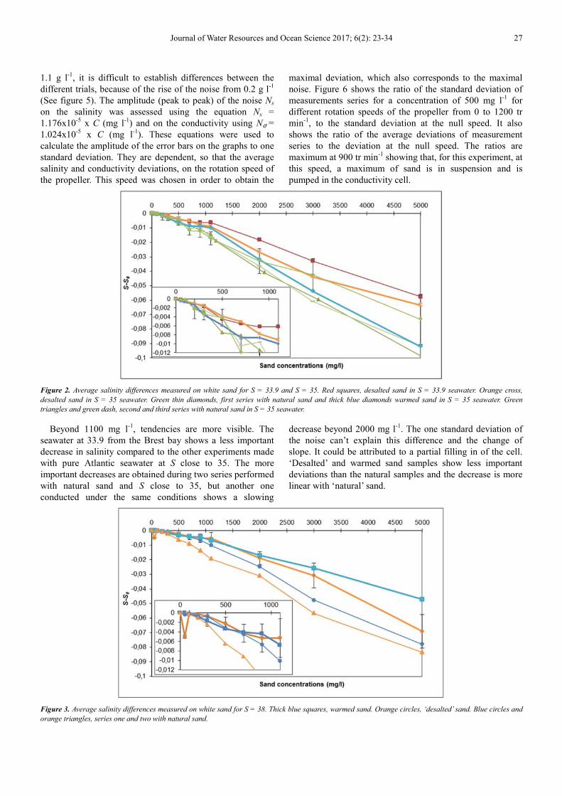
Figure 2. Average salinity differences measured on white sand for S = 33.9 and S = 35. Red squares, desalted sand in S = 33.9 seawater. Orange cross,
desalted sand in S = 35 seawater. Green thin diamonds, first series with natural sand and thick blue diamonds warmed sand in S = 35 seawater. Green
triangles and green dash, second and third series with natural sand in S = 35 seawater.
Beyond 1100 mg l-1
, tendencies are more visible. The
seawater at 33.9 from the Brest bay shows a less important
decrease in salinity compared to the other experiments made
with pure Atlantic seawater at S close to 35. The more
important decreases are obtained during two series performed
with natural sand and S close to 35, but another one
conducted under the same conditions shows a slowing
decrease beyond 2000 mg l-1
. The one standard deviation of
the noise can’t explain this difference and the change of
slope. It could be attributed to a partial filling in of the cell.
‘Desalted’ and warmed sand samples show less important
deviations than the natural samples and the decrease is more
linear with ‘natural’ sand.
Figure 3. Average salinity differences measured on white sand for S = 38. Thick blue squares, warmed sand. Orange circles, ‘desalted’ sand. Blue circles and
orange triangles, series one and two with natural sand.

28 Marc Le Menn and Laurent Pacaud: Effect of Sediment Suspensions on Seawater Salinity Assessments
Figure 3 shows the results obtained with Mediterranean seawater. The less important deviations obtained with ‘desalted’ and
warmed sand are more visible.
Figure 4. Average salinity differences measured on ‘natural’ white sand for S = 35 and S = 38. Blue circles and triangles, S = 38. Green diamonds, dash and
triangles, S = 35.
Figure 4, shows series with ‘natural’ sand for S = 35 and S
= 38. The effect of sand on seawater conductivity is slightly
less important at higher salinities (for the waters at 38 and
35). According to Revil et al. [25], the ζ potential, which
represents the electrical potential at the mineral/water
interface, decreases with increasing salinity (but it increases
with temperature and pH). This explanation is not verified on
figure n° 2 for SP = 33.9, probably because this water has a
composition or a pH different from the standard one’s and the
sand samples have been ‘desalted’. According to these
measurements, for SP = 35, the salinity error starts to be
superior to 0.002 from 250 mg l-1
and is close to 0.1 at 5000
mg l-1
. 0.002 is the uncertainty expected on practical salinity
measurements in open oceans, and it will be considered as a
threshold in this document.
At the end of the measurement series, the stirring propeller
is stopped and other measurements are made to know the
evolution of the salinity as the sand deposits on the bottom of
the container. The salinity retrieves its initial value with
0.003 to 0.005 units more, with the ‘natural’ and the
‘desalted’ sand. This increase can’t be attributed to
evaporation because other measurements have been made
with the stirring propeller operating for a duration of several
hours, showing that evaporation is negligible. The only
possible explanations are that the circulation of the sand
through the cell or that the mixing of sand in the seawater
slightly modify the ionic activity of the water.
Figure 5. Noize on the practical salinity of a seawater measured with an SBE 37, as the (natural) sand concentration increases.

Journal of Water Resources and Ocean Science 2017; 6(2): 23-34 29
Figure 6. Red squares, ratio of the standard deviation of measurements series for a concentration of 500 mg l-1 for different rotation speeds of the propeller
from 0 to 1200 tr.min-1, to the standard deviation at the null speed. Blue diamond, ratio of the average deviations of measurement series to the deviation at the
null speed. The optimal speed is 900 tr min-1.
The same experiment was conducted using mud taken
from two different estuaries of the West of France (Abers
Benoit, called A, and Le Faou bay, called F) and seawater
salinities close to 34 (water from Brest bay). Figure 7 shows
the results. These are almost equivalent to the former results,
but as the composition of these muds is not known, they
cannot be generalized. A change of slope is also visible
beyond 1000 mg l-1
. Contrary to the results obtained with the
pure sand, the desalted mud A and F shows important
conductivity decreases. The dried grains of mud showed a
high static repulsion in the glass cupel during the weighing.
That could perhaps explain this change of response.
Figure 7. Salinity differences measured on two different muds and a seawater salinity close to 34. Red square, natural mud F, blue cross, natural mud A,
orange circle, desalted mud A, blue plus, desalted mud F. The error bars represent the standard deviation of the noise.
4. Explanation of Effects on Conductivity
Measurements
P. Held et al. [14] have described a ‘blinding effect’ which
occurs when the cross section of a conductivity cell is
reduced by sediments. They have tried to demonstrate that
this effect is independent on the geometry of the cell and that
it depends partially on the conductivity of the sediments, but
they didn’t try to fit their relation to the observed deviations.
They write that, at a given temperature (25 °C) σM = σref
VW,susp / V0 where VW,susp is the water volume in suspension,
30 Marc Le Menn and Laurent Pacaud: Effect of Sediment Suspensions on Seawater Salinity Assessments
σref the conductivity and V0 the volume of a reference
solution. In our case, σref = σW and VW,susp = (VW – Vs) where
VS is the added volume of sand. That gives σM = σW (1 –
Vs/VW). This relation applied to our experiments shows
relative errors for ‘natural’ sand between 0.04 and 1.62 for Sp
= 35 and between 0.062 and 2.00 for Sp = 38. Moreover, the
changes of slope and the differences observed between the
‘natural’ and the ‘desalted’ sand cannot be explained.
In order to take these remarks into account, we replaced
VW by VC the volume of the conductivity cell. The measured
resistance RM of a Sea-Bird conductivity cell is:
cMM
V
lR
2
1 2
σ= (9)
where l is the length of the cell. If we consider the sum of
conductances (RM)-1
= (RW)-1
+ (RS)-1
, RW being the resistance
of the seawater and RS the resistance of the sediments, we
have:
( ) SCSSCCwM VVVR 22 σσ +−= (10)
where VSC is the volume of sand in the cell. Equating
relations (9) and (10), leads us to write the relation:
C
SCS
C
SCwM
V
V
V
V σσσ +
−= 1 (11)
In the case of clean sand, σS can be replaced by the relation
(5). For sediments containing clay, the relation (7) could be
used instead of the relation (5) and for clayed materials with
a CEC, the relation (8) could be used in the same way. The
relation (11) therefore becomes:
−−=
FF
S
V
V Wn
C
SCwM 11σσ (12)
It is then necessary to define the value of VSC. We can
write that the volume of sand VS in the container, multiplied
by the efficiency ε of pumping, is proportional to the volume
of sand in the cell VSC:
SC
S
C
T
V
V
V
V ε= (13)
where VT = VW + VS is the total volume of the mixture. We
have therefore:
SW
SCSC
VV
VVV
+= ε (14)
We can divide by VS and, as VS can be hardly measured,
we can write that VS = mS/ρS where ms is the added mass of
sand and ρS its density: ρS = 1.85 g cm-3
. The relation (14)
becomes:
S
SW
S
WC
SC
m
V
V
VV
V
ρεε
+=
+=
11
(15)
The value of VSC/VC can be replaced in the relation (12) to
give:
−
+−=
FF
S
V
V
Wn
S
WwM 1
1
1εσσ (16)
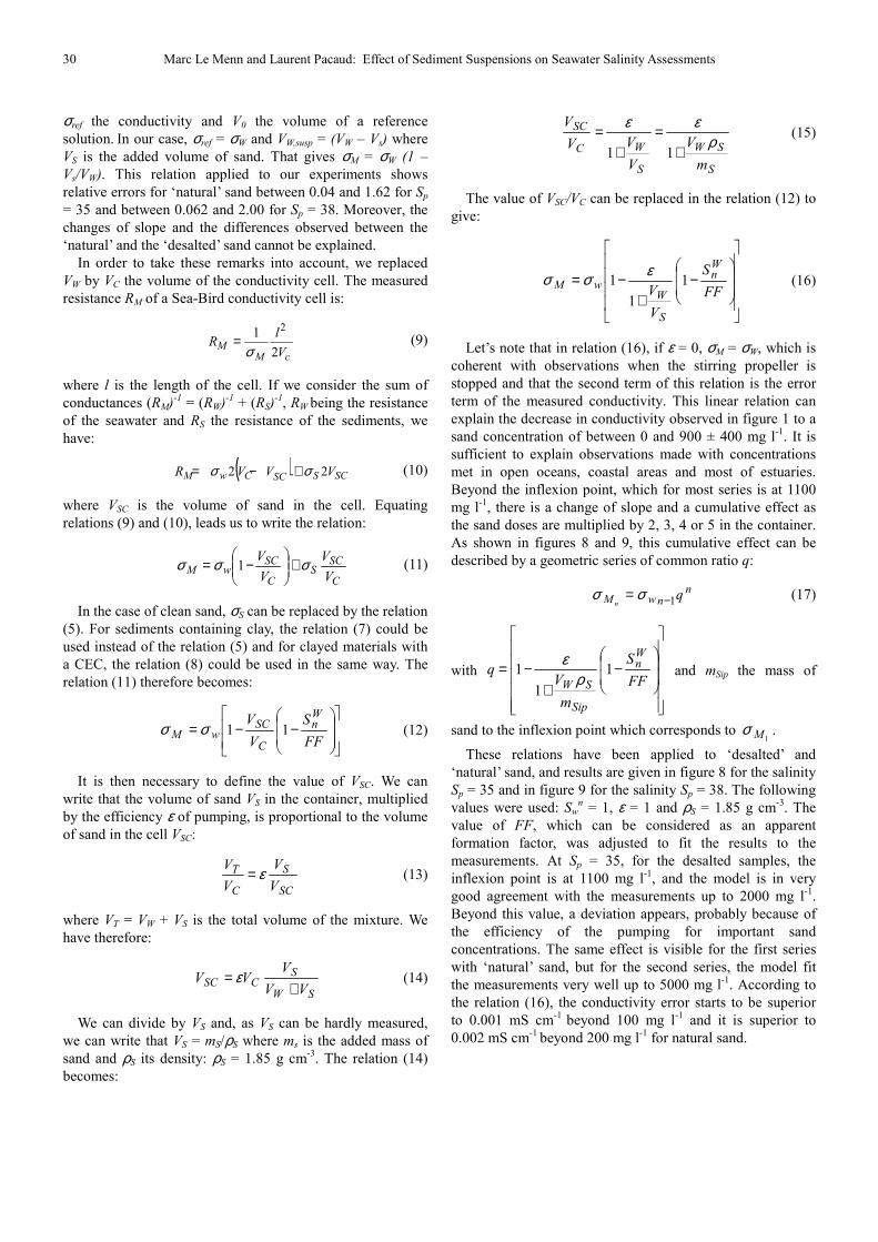
Let’s note that in relation (16), if ε = 0, σM = σW, which is
coherent with observations when the stirring propeller is
stopped and that the second term of this relation is the error
term of the measured conductivity. This linear relation can
explain the decrease in conductivity observed in figure 1 to a
sand concentration of between 0 and 900 ± 400 mg l-1
. It is
sufficient to explain observations made with concentrations
met in open oceans, coastal areas and most of estuaries.
Beyond the inflexion point, which for most series is at 1100
mg l-1
, there is a change of slope and a cumulative effect as
the sand doses are multiplied by 2, 3, 4 or 5 in the container.
As shown in figures 8 and 9, this cumulative effect can be
described by a geometric series of common ratio q:
nnwM q
n 1−= σσ (17)
with
−
+−=
FF
S
m
Vq
Wn
Sip
SW
1
1
1ρ
ε and mSip the mass of
sand to the inflexion point which corresponds to 1Mσ .
These relations have been applied to ‘desalted’ and
‘natural’ sand, and results are given in figure 8 for the salinity
Sp = 35 and in figure 9 for the salinity Sp = 38. The following
values were used: Swn = 1, ε = 1 and ρS = 1.85 g cm
-3. The
value of FF, which can be considered as an apparent
formation factor, was adjusted to fit the results to the
measurements. At Sp = 35, for the desalted samples, the
inflexion point is at 1100 mg l-1
, and the model is in very
good agreement with the measurements up to 2000 mg l-1
.
Beyond this value, a deviation appears, probably because of
the efficiency of the pumping for important sand
concentrations. The same effect is visible for the first series
with ‘natural’ sand, but for the second series, the model fit
the measurements very well up to 5000 mg l-1
. According to
the relation (16), the conductivity error starts to be superior
to 0.001 mS cm-1
beyond 100 mg l-1
and it is superior to
0.002 mS cm-1
beyond 200 mg l-1
for natural sand.
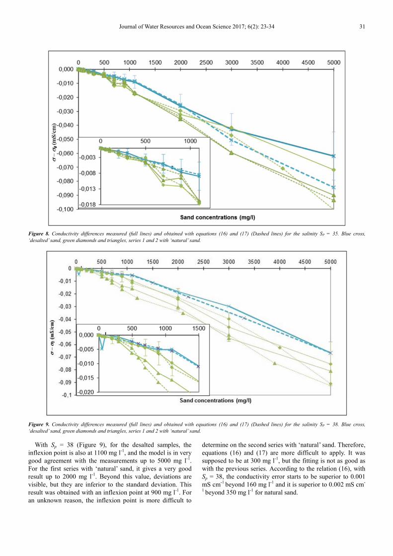
Journal of Water Resources and Ocean Science 2017; 6(2): 23-34 31
Figure 8. Conductivity differences measured (full lines) and obtained with equations (16) and (17) (Dashed lines) for the salinity SP = 35. Blue cross,
‘desalted’ sand, green diamonds and triangles, series 1 and 2 with ‘natural’ sand.
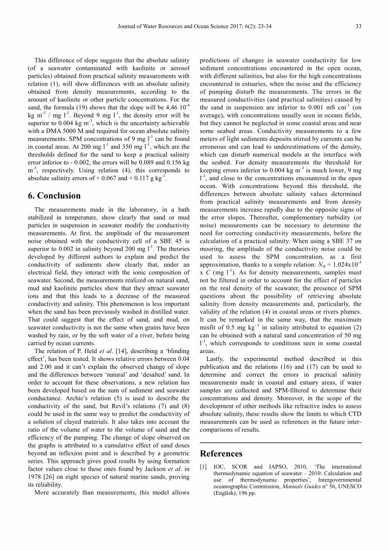
Figure 9. Conductivity differences measured (full lines) and obtained with equations (16) and (17) (Dashed lines) for the salinity SP = 38. Blue cross,
‘desalted’ sand, green diamonds and triangles, series 1 and 2 with ‘natural’ sand.
With Sp = 38 (Figure 9), for the desalted samples, the
inflexion point is also at 1100 mg l-1
, and the model is in very
good agreement with the measurements up to 5000 mg l-1
.
For the first series with ‘natural’ sand, it gives a very good
result up to 2000 mg l-1
. Beyond this value, deviations are
visible, but they are inferior to the standard deviation. This
result was obtained with an inflexion point at 900 mg l-1
. For
an unknown reason, the inflexion point is more difficult to
determine on the second series with ‘natural’ sand. Therefore,
equations (16) and (17) are more difficult to apply. It was
supposed to be at 300 mg l-1
, but the fitting is not as good as
with the previous series. According to the relation (16), with
Sp = 38, the conductivity error starts to be superior to 0.001
mS cm-1
beyond 160 mg l-1
and it is superior to 0.002 mS cm-
1 beyond 350 mg l
-1 for natural sand.

32 Marc Le Menn and Laurent Pacaud: Effect of Sediment Suspensions on Seawater Salinity Assessments
Table 1. Values of the formation factor FF used to obtain the results of
figures 8 and 9, and the corresponding porosities φ.
Sand Sp FF φ Desalted 35.10 1.59 0.73
Natural 35.09 1.40 0.80
Natural 35.13 1.84 0.67
Desalted 37.97 1.30 0.84
Natural 37.87 1.40 0.80
Natural 37.96 1.35 0.82
Table 1 shows the different values of FF used to calculate
the fitting curves of figures 8 and 9. They correspond (with
one exception) with the values obtained experimentaly by
Jackson et al. in 1978 [26], on eight natural marine sands.
They used a sand-settling cell with a large sediment chamber
above which there was a graduated cylinder full of water and
acting as an accurate volume measuring device. The chamber
was equiped with electrodes used as a four-electrode method.
With this apparatus, they found FF values between 1.39 and
1.58. That confirms the validity of equations (16) and (17).
During the measurements, the humidity of the room was
measured in order to determine its influence on the slopes of
the curves, but no correlation was found between the
variations of FF and the humidity of the air, which could
have changed the ζ potential of the sand before its mixing
with the seawater.
5. Effect of SPM on Seawater Density
Measurements
Grains of sand are not easy to keep in suspension and it is
hardly difficult to take a sample from a solution in order to
measure its density with a vibrating tube meter like an Anton
Paar DMA 5000. To show the effect of SPM on density
measurements, we used white kaolin powder. Kaolin
particles are not soluble in water and they can be easily kept
in suspension. Among the different components of shale,
kaolinite has the lower CEC (between 3 – 15 meq/100 g). It
is a non-expanding silicate clay composed of a superposition
of tetrahedral sheets containing Si and O atoms and of
octahedral sheets containing Al – OH bounds. Kaolin powder
particle sizes range between 0.1 and 80 µm according to
Comparon [27]. This range of sizes is similar, for example, to
aerosol particles which can be collected in the North Atlantic
Ocean, as collected in 2003 by Buck et al. [28]. It is also
similar to the range of sizes found in the Mediterranean Sea
by Bressac et al. in 2011 [29] after Saharan dust depositions.
These depositions can occur over large areas.
When kaolin powder is mixed with seawater with a
salinity of 33.9, the conductivity of the solution decreases
strongly, following a slope like desalted mud A in figure 7.
Its value is: dσ/dC = - 3.4x10⁻⁵
mS cm-1
/mg l-1
or dS/dC = -
3.15x10⁻⁵
g kg-1
/mg l-1
. Inversely, the densities measured with
a DMA 5000 M follow a positive slope dρ/dC = 5.88 10-4
kg
m-3
/mg l-1
. This slope can be accurately retrieved by
calculating the density ρS of the solution:
( )T
KWS
V
mm +=ρ (18)
where mW is the mass of water and mK the mass of kaolinite.
Using ρK, the kaolinite density, which is 2.65 kg m-3
, relation
(18) becomes:
( )
+−= KKKT
K
W
TS mmV
Vρ
ρρ
ρ 1 (19)
Figure 10 shows the density deviations obtained with
measured values of different kaolinite solutions and the same
deviations obtained with formula (19). Taking into account
the measurement uncertainties, the agreement between the
measured values and the calculated values is very good.
Figure 10. Blue squares, density deviations in kg m-3 measured with an Anton Paar DMA 5000 M. Brown triangles, density deviations calculated with relation
(19).
Journal of Water Resources and Ocean Science 2017; 6(2): 23-34 33
This difference of slope suggests that the absolute salinity
(of a seawater contaminated with kaolinite or aerosol
particles) obtained from practical salinity measurements with
relation (1), will show differences with an absolute salinity
obtained from density measurements, according to the
amount of kaolinite or other particle concentrations. For the
sand, the formula (19) shows that the slope will be 4.46 10-4
kg m-3
/ mg l-1
. Beyond 9 mg l-1
, the density error will be
superior to 0.004 kg m-3
, which is the uncertainty achievable
with a DMA 5000 M and required for ocean absolute salinity
measurements. SPM concentrations of 9 mg l-1
can be found
in coastal areas. At 200 mg l-1
and 350 mg l-1
, which are the
thresholds defined for the sand to keep a practical salinity
error inferior to - 0.002, the errors will be 0.089 and 0.156 kg
m-3
, respectively. Using relation (4), this corresponds to
absolute salinity errors of + 0.067 and + 0.117 g kg-1
.
6. Conclusion
The measurements made in the laboratory, in a bath
stabilized in temperature, show clearly that sand or mud
particles in suspension in seawater modify the conductivity
measurements. At first, the amplitude of the measurement
noise obtained with the conductivity cell of a SBE 45 is
superior to 0.002 in salinity beyond 200 mg l-1
. The theories
developed by different authors to explain and predict the
conductivity of sediments show clearly that, under an
electrical field, they interact with the ionic composition of
seawater. Second, the measurements realized on natural sand,
mud and kaolinite particles show that they attract seawater
ions and that this leads to a decrease of the measured
conductivity and salinity. This phenomenon is less important
when the sand has been previously washed in distilled water.
That could suggest that the effect of sand, and mud, on
seawater conductivity is not the same when grains have been
washed by rain, or by the soft water of a river, before being
carried by ocean currents.
The relation of P. Held et al. [14], describing a ‘blinding
effect’, has been tested. It shows relative errors between 0.04
and 2.00 and it can’t explain the observed change of slope
and the differences between ‘natural’ and ‘desalted’ sand. In
order to account for these observations, a new relation has
been developed based on the sum of sediment and seawater
conductance. Archie’s relation (5) is used to describe the
conductivity of the sand, but Revil’s relations (7) and (8)
could be used in the same way to predict the conductivity of
a solution of clayed materials. It also takes into account the
ratio of the volume of water to the volume of sand and the
efficiency of the pumping. The change of slope observed on
the graphs is attributed to a cumulative effect of sand doses
beyond an inflexion point and is described by a geometric
series. This approach gives good results by using formation
factor values close to these ones found by Jackson et al. in
1978 [26] on eight species of natural marine sands, proving
its reliability.
More accurately than measurements, this model allows
predictions of changes in seawater conductivity for low
sediment concentrations encountered in the open ocean,
with different salinities, but also for the high concentrations
encountered in estuaries, when the noise and the efficiency
of pumping disturb the measurements. The errors in the
measured conductivities (and practical salinities) caused by
the sand in suspension are inferior to 0.001 mS cm-1
(on
average), with concentrations usually seen in oceans fields,
but they cannot be neglected in some coastal areas and near
some seabed areas. Conductivity measurements to a few
meters of light sediments deposits stirred by currents can be
erroneous and can lead to underestimations of the density,
which can disturb numerical models at the interface with
the seabed. For density measurements the threshold for
keeping errors inferior to 0.004 kg m-3
is much lower, 9 mg
l-1
, and close to the concentrations encountered in the open
ocean. With concentrations beyond this threshold, the
differences between absolute salinity values determined
from practical salinity measurements and from density
measurements increase rapidly due to the opposite signs of
the error slopes. Thereafter, complementary turbidity (or
noise) measurements can be necessary to determine the
need for correcting conductivity measurements, before the
calculation of a practical salinity. When using a SBE 37 on
mooring, the amplitude of the conductivity noise could be
used to assess the SPM concentration, as a first
approximation, thanks to a simple relation: Nσ = 1.024x10⁻⁵
x C (mg l-1
). As for density measurements, samples must
not be filtered in order to account for the effect of particles
on the real density of the seawater, the presence of SPM
questions about the possibility of retrieving absolute
salinity from density measurements and, particularly, the
validity of the relation (4) in coastal areas or rivers plumes.
It can be remarked in the same way, that the maximum
misfit of 0.5 mg kg−1
in salinity attributed to equation (2)
can be obtained with a natural sand concentration of 50 mg
l-1
, which corresponds to conditions seen in some coastal
areas.
Lastly, the experimental method described in this
publication and the relations (16) and (17) can be used to
determine and correct the errors in practical salinity
measurements made in coastal and estuary areas, if water
samples are collected and SPM-filtered to determine their
concentrations and density. Moreover, in the scope of the
development of other methods like refractive index to assess
absolute salinity, these results show the limits to which CTD
measurements can be used as references in the future inter-
comparisons of results.
References
[1] IOC, SCOR and IAPSO, 2010, ‘The international thermodynamic equation of seawater – 2010: Calculation and use of thermodynamic properties’, Intergovernmental oceanographic Commission, Manuals Guides n° 56, UNESCO (English), 196 pp.
34 Marc Le Menn and Laurent Pacaud: Effect of Sediment Suspensions on Seawater Salinity Assessments
[2] Millero J. F., Pierrot D., 2002, ‘Speciation of metals in natural seawaters’, Chapter in Chemistry of Marine Water and Sediments, 193-220.
[3] Millero F. J., Feistel R., Wright D. G., MacDougall T. J., 2008a, ‘The composition of standard seawater and the definition of the reference – composition salinity scale’, Deep-Sea Res. I, 55, 10-72.
[4] Pawlowicz R., Wright D. G., and F. J. Millero, 2011, ‘The effects of biogeochemical processes on oceanic conductivity/salinity/density relationships and the characterization of real seawater’, Ocean Sci., 7, 363–387.
[5] Wright D. G., Pawlowicz R., McDougall T. J., Feistel R., and Marion G. M., 2011, ‘Absolute Salinity, “Density Salinity” and the Reference-Composition Salinity Scale: present and future use in the seawater standard TEOS-10’, Ocean Sci., 7, 1–26.
[6] Millero J. F., 1978, ‘The physical chemistry of Baltic Sea waters’, Thalass Jugosl., 14, 1-46.
[7] Millero F. J., Waters, J., Woosley R. J., Huang F., Chanson M., 2008b, ‘The effect of composition on the density of Indian Ocean waters’, Deep-Sea Res. I, 55, 460-470.
[8] Millero J. F., Huang F., 2009, ‘The density of seawater as a function of salinity (5 to 70 gkg-1) and temperature (273.15 to 263.15 K), Ocean Sci., 5, 91-100.
[9] Millero J. F., Huang F., Woosley R. J., Letscher R. T., Hansell D. A., 2011, ‘Effect of dissolved organic carbon and alkalinity on the density of Arctic Ocean waters’, Aquat. Geochem., 17, 311-326.
[10] Woosley R. J., Huang F., Millero F. J., 2014, ‘Estimating absolute salinity (SA) in the world’s oceans using density and composition’, Deep-Sea Res. I, 93, 14-20.
[11] MacDougall T. J., Jackett D. R., Millero J. F., Pawlowicz R., Barker P. M., 2012, ‘A global algorithm for estimating absolute salinity’, Ocean Sci., 8, 1123-1134.
[12] Pawlowicz R., Feistel R., McDougall T. J., Ridout P., Wolf H., 2016, ‘Metrological challenges for measurements of key climatological observables Part 2: oceanic salinity’, Metrologia, 53, R12-R25.
[13] Pawlowicz R., 2015, ‘The absolute salinity of seawater diluted by river water’, Deep-Sea Research I, 101, 71-79.
[14] Held P., Kegler P., Schrottke K., 2014, ‘Influence of suspended particulate matter on salinity measurements’, Continental Shelf Research 85, 1-8, DOI: 10.1016/j.csr.2014.05.014.
[15] Archie G. E., 1942, ‘The electrical resistivity log as an aid in determining some reservoir characteristics’, Petroleum Transactions of the AIME 146, 54-62.
[16] Revil A., Glover P. W. J., 1998, ‘Nature of surface electrical
conductivity in natural sands, sandstone, and clays’, Geophys. Res. Let., 25, 5, 691-694.
[17] Revil A., Glover P. W. J., 1997-I, ‘Theory of ionic-surface electrical conduction in porous media’, Physical Review B, 55, 3, 1757-1773.
[18] Waxman M. H., and Smits L. J. M., 1968, ‘Electrical conductivities in oil-bearing shaly sands’, Society of Petroleum Engineer Journal, 107-122
[19] Johnson D. L., Plona T. J., Kojima H., 1986, Proceedings of the second international symposium on the physics and chemistry of porous media, in Physics and Chemistry of Porous Media-II (Ridgefield), edited by Banavar J. R., Koplik J. and Winkler K. W., AIP Conf. Proc. N° 154.
[20] Leroy P., Devau N., Revil A., Bizi M., 2013, ‘Influence of surface conductivity on the apparent zeta potential of amorphous silica nanoparticles’, http://dx.doi.org/10.1016/j.jcis.2013.08.012.
[21] Leroy P., Revil A., Kemna A., Cosenza P., Ghorbani A., 2008, ‘Complex conductivity of water-saturated packs of glass beads’, Journal of Colloid and Interface Science, 321, 103-117.
[22] Revil A., Skold M., 2011, ‘Salinity dependence of spectral induced polarization in sands and sandstones’, Geophys. J. Int., 187, 813-824.
[23] Revil A., Linde N., Cerepi A., Jougnot D., Matthäi S., Finsterle S., 2007, ‘Electro-kinetic coupling in unsaturated porous media’, Journal of Colloid and Interface Science, 313, 1, 315-327.
[24] Revil A., 2013, ‘Effective conductivity and permittivity of unsaturated porous materials in the frequency range 1 mHz – 1 GHz’, Water Resources Research, 49, 306 – 327.
[25] Revil A., Pezard P. A., 1999, ‘Streaming potential in porous media. 1. Theory of the zeta potential’, Journal of geophysical research, 104, B9, 20,021-20,031.
[26] Jackson P. D., Taylor Smith D., Stanford P. N., 1978, ‘Resistivity-porosity-particle shape relationships for marine sands’, Geophysics, 43, 6, 1250-1268.
[27] Comparon L., 2005, Etude expérimentale des propriétés électriques et diélectriques des matériaux argileux consolidés’, Institut de Physique du Globe de Paris and B. R. G. M. theses.
[28] Buck C. S., Landing W. M., Resing J. A., 2010, ‘Particle size and aerosol iron solubility: a high-resolution analysis of Atlantic aerosols’, Marine Chemistry, 120, 1-4, 14-24.
[29] Bressac M., Guieu C., Doxaran D., Bourrin F., Obolensky G., Grisoni J.-M., 2012, ‘A mesocosm experiment coupled with optical measurements to assess the fate and sinking of atmospheric particles in clear oligotrophic waters’, Geo-Mar Letter, 32: 153-164.