effect of pipe inclination angle on gas liquid flow …
TRANSCRIPT

EFFECT OF PIPE INCLINATION ANGLE ON GAS–LIQUID FLOW USING
ELECTRICAL CAPACITANCE TOMOGRAPHY (ECT) DATA
A Thesis Presented to the Department of
Petroleum Engineering
The African University of Science and Technology
In Partial Fulfilment of the Requirements
For the Degree of
MASTER OF SCIENCE
By
OTENG BISMARK
Abuja, Nigeria
December, 2014

ii
EFFECT OF PIPE INCLINATION ANGLE ON GAS–LIQUID FLOW USING
ELECTRICAL CAPACITANCE TOMOGRAPHY (ECT) DATA
By
OTENG BISMARK
RECOMMENDED:
Supervisor, Dr. Mukhtar Abdulkadir
Professor Wumi Iledare
Dr. Alpheus Igbokoyi
APPROVED:
Head, Department of Petroleum Engineering
Chief Academic Officer
DATE

iii
BISMARK OTENG© Copyright by [2014]
All Rights Reserved

iv
ABSTRACT
Pipes that make up oil and gas wells are not vertical but could be inclined at any angle
between vertical and the horizontal which is a significant technology of modern drilling-
Experimental data on time varying liquid holdup for and pipe inclination angles were
analyzed and interpreted. Parameters such as void fraction, slug frequency, lengths of liquid slug,
Taylor bubble and slug unit, structure velocity and pressure drop were calculated from the
experimental data. It was observed that an increase in pipe inclination from 0o to 30
o brings
about a corresponding reduction in average void fraction. Moreover, there is no particular
correlation that gave better results in the two inclination angles based on the drift -flux model
considered. The results of the comparison between the pressure gradient concerned with the 0o
and 30o pipe inclination angles considered in this study using the Beggs and Brill (1973)
correlation showed that the total pressure gradient increases with an increase in pipe inclination
as a consequence of an increase in both gravitational and frictional pressure gradient. This study
has provided useful information of the effect of pipe inclination on void fraction distribution
using electrical capacitance tomography (ECT) data.

v
ACKNOWLEDGEMENT
To my God who has been my glory and lifter-up of my head, I cannot thank you enough on this
page, unto you be all the glory and honor forever more for bringing me this far. I could not
simply have made it without you. My sincere gratitude goes to my supervisor Dr. Mukhtar
Abdulkadir whose relentless effort has made this work a success, thank you sir for making it be.
My next appreciation goes to my committee members Professor Wumi Iledera and Dr. Alpheus
Igbokoyi; I appreciate your supports so much. To my parents and siblings especially my senior
brother, Emmanuel Oteng, whose resources have made me come this far, may God reward you
bountifully. I would not forget all the numerous friends and loved ones whose encouragements
and supports saw me through my stay in AUST especially Deborah Boadu, when it looked
impossible, you reminded me of the God under whose care there is nothing impossible; God
richly bless you. Then to the Petroleum Engineering class of 2013/14, I say your support
has been great. My gratitude goes to the multiphase flow in pipe group members for their
unfailing support.

vi
DEDICATION
I dedicate this work to my parents and siblings, whose love, support and encouragement I can
never forget.

vii
Contents December, 2014 ............................................................................................................................................. i
ABSTRACT ................................................................................................................................................. iv
ACKNOWLEDGEMENT ............................................................................................................................ v
DEDICATION ............................................................................................................................................. vi
LIST OF FIGURES ...................................................................................................................................... x
LIST OF TABLES ...................................................................................................................................... xii
Chapter 1 ....................................................................................................................................................... 1
1.1 Introduction ....................................................................................................................................... 1
1.3 Problem statement ............................................................................................................................. 4
1.4 Aim and Objectives ........................................................................................................................... 5
1.5 Structure of the thesis ........................................................................................................................ 5
Chapter 2 ....................................................................................................................................................... 7
LITERATURE REVIEW ............................................................................................................................. 7
2.1 Gas-liquid flow in inclined pipes ...................................................................................................... 7
2.2 Flow regime classification .............................................................................................................. 12
2.2.1 Vertical flow regimes .............................................................................................................. 13
2.2.1.1 Bubble flow pattern ............................................................................................................ 14
2.2.1.2 Slug flow pattern ................................................................................................................ 14
2.2.1.3 Churn flow pattern ............................................................................................................. 15
2.2.1.4 Annular flow pattern ....................................................................................................... 15
2.2.2 Horizontal flow regimes ........................................................................................................ 16
2.2.2.1 Bubbly flow- ...................................................................................................................... 16
2.2.2.2 Stratified flow- ................................................................................................................... 16
2.2.2.3 Stratified-wavy flow- .......................................................................................................... 17
2.2.2.4 Plug flow- ........................................................................................................................... 17
2.2.2.5 Slug flow- ........................................................................................................................... 17
2.2.2.6 Annular flow- ..................................................................................................................... 17
2.2.2.7 Mist flow- ........................................................................................................................... 18
2.2.3 Flow pattern maps .................................................................................................................. 18
2.2.3.1 Baker flow pattern map ...................................................................................................... 19
2.2.4 Flow pattern identification ..................................................................................................... 20

viii
2.3 Tomographic techniques ................................................................................................................. 25
2.4 Void fraction ................................................................................................................................... 26
2.4.1 Concept of void fraction ......................................................................................................... 27
2.4.2 Classification of void fraction ................................................................................................. 28
2.4.3 The measurement principle ..................................................................................................... 30
2.5 Void fraction correlations for inclined pipes .................................................................................. 31
2.6 Drift flux correlations...................................................................................................................... 32
2.7 Pressure drop in two-phase inclined pipes ...................................................................................... 33
Chapter 3 ..................................................................................................................................................... 35
DATA ACQUISITION SETUP.................................................................................................................. 35
3.1 Overview of the experimental facility............................................................................................. 35
3.2 System (test fluid) ........................................................................................................................... 37
3.3 Parameters determined for this present study ................................................................................ 38
3.3.1 Translational or rise velocity of Taylor bubble (structure velocity) ....................................... 38
3.3.2 Determination of the distance (∆L) between the two ECT planes .......................................... 39
3.3.3 Determination of time delay ................................................................................................... 39
3.3.4 Slug frequency ........................................................................................................................ 40
3.3.5 Lengths of the slug unit, the Taylor bubble and the liquid slug .............................................. 41
3.4 Summary ........................................................................................................................................ 42
CHAPTER 4 ............................................................................................................................................... 43
RESULTS AND DISCUSSION ................................................................................................................. 43
4.1 Analysis of length; liquid slug, Taylor bubble and slug unit .......................................................... 43
4.2 Time and space average analysis .................................................................................................... 47
4.2.1 Mean void fraction from empirical correlations ..................................................................... 50
4.3 Void fraction analysis ..................................................................................................................... 53
4.4 Pressure drop ................................................................................................................................... 57
4.5 Structure velocity ............................................................................................................................ 60
4.6 Flow pattern map ............................................................................................................................ 62
4.7 Probability density function (PDF) ................................................................................................. 64
4.8 Frequency ........................................................................................................................................ 67
CHAPTER 5 ............................................................................................................................................... 70
CONCLUSIONS AND RECOMMENDATIONS ..................................................................................... 70

ix
5.1 Conclusions .................................................................................................................................... 70
5.2 Recommendations .......................................................................................................................... 71
NOMENCLATURE ................................................................................................................................... 72
APPENDICES ............................................................................................................................................ 74
APPENDIX A DATA TEST MATRIX FOR 67mm 0o PIPE INCLINATION .................................... 74
APPENDIX B DATA TEST MATRIX FOR 67mm 30o PIPE INCLINATION ................................... 77
APPENDIX C BEGGS AND BRILL (1973) CORRELATION FOR PRESSURE GRADIENT ............ 81
CORRELATION PREDICTION FOR 67mm 0o PIPE INCLINATION .............................................. 81
APPENDIX D BEGGS AND BRILL (1973) CORRELATION FOR PRESSURE GRADIENT ............ 83
CORRELATION PREDICTION FOR 67mm 30o PIPE INCLINATION ........................................... 83
REFERENCES ........................................................................................................................................... 86

x
LIST OF FIGURES
Figure 2.1 -Upward vertical flow pattern- Taitel et al. (1980) ............................................................. 14
Figure 2.2 Vertical flow patterns Abbas (2010) ................................................................................... 16
Figure 2.3 Flow- patterns- in- horizontal- gas-liquid -flows- Taitel (2000) ......................................... 18
Figure 2.4 Baker (1954) flow pattern map for horizontal flow in a tube. ............................................ 20
Figure 2.5 a, b, c Flow identification by power spectrum density of pressure gradient Hubbard and
Dukler (1966). Adapted from Hewitt (1978) .............................................................................................. 21
Figure 2.6 Flow pattern identification by probability distribution function of void fraction Jones and
Zuber (1975)……………... ........................................................................................................................ 22
Figure 2.6 (a) a single peak at low void fraction is indicative of discrete bubble flow ....................... 23
Figure 2.6 (b) a single peak at low void fraction accompanied by a long tail is indicative spherical
cap bubble……….. ..................................................................................................................................... 23
Figure 2.6 (c) a double peak feature with the higher peak at low void fraction and the lower peak at a
higher void fraction signifies stable slug flow ............................................................................................ 24
Figure 2.6 (d) a double peak feature with the lower peak at low void fraction and the higher peak at a
higher void fraction signifies unstable slug flow ........................................................................................ 24
Figure 2.6 (e) a single peak at a high void fraction with a broadening tail is indicative of churn flow 25
Figure 2.6 (f) a single high peak at high void fraction is defined as annular flow ............................. 25
Figure 3. 1 The components of the rig (a) liquid pump (b) liquid tank (c) air-silicone oil mixing
section (d) rotameters and (e) cyclone separator Abdulkadir (2011)………………………………..36
Figure 3.2 Experimental flow facility Abdulkadir (2011b) .................................................................. 37
Figure 3.3 Void fraction time series from the two ECT probes ........................................................... 40
Figure 4.1 a plot of length of liquid slug against gas superficial velocity for various liquid superficial
velocities…………………………………………………………………………………………. 44
Figure 4.2 a plot of length of slug unit against gas superficial velocity for various liquid superficial
velocities…………………….. ................................................................................................................... 45
Figure 4.3 a plot of length of Taylor bubble against gas superficial velocity for various liquid
superficial velocities ................................................................................................................................... 46
Figure 4.4 Effect of gas superficial velocity and angle of inclination on average void fraction at
different liquid superficial velocity ............................................................................................................. 49

xi
Figure 4.5 (a) Experimental void fraction against empirical models for the inclination ................. 50
Figure 4. 5 (b) Experimental void fraction against empirical models for the inclination .............. 51
Figure 4.6 RMS of empirical correlation ............................................................................................. 52
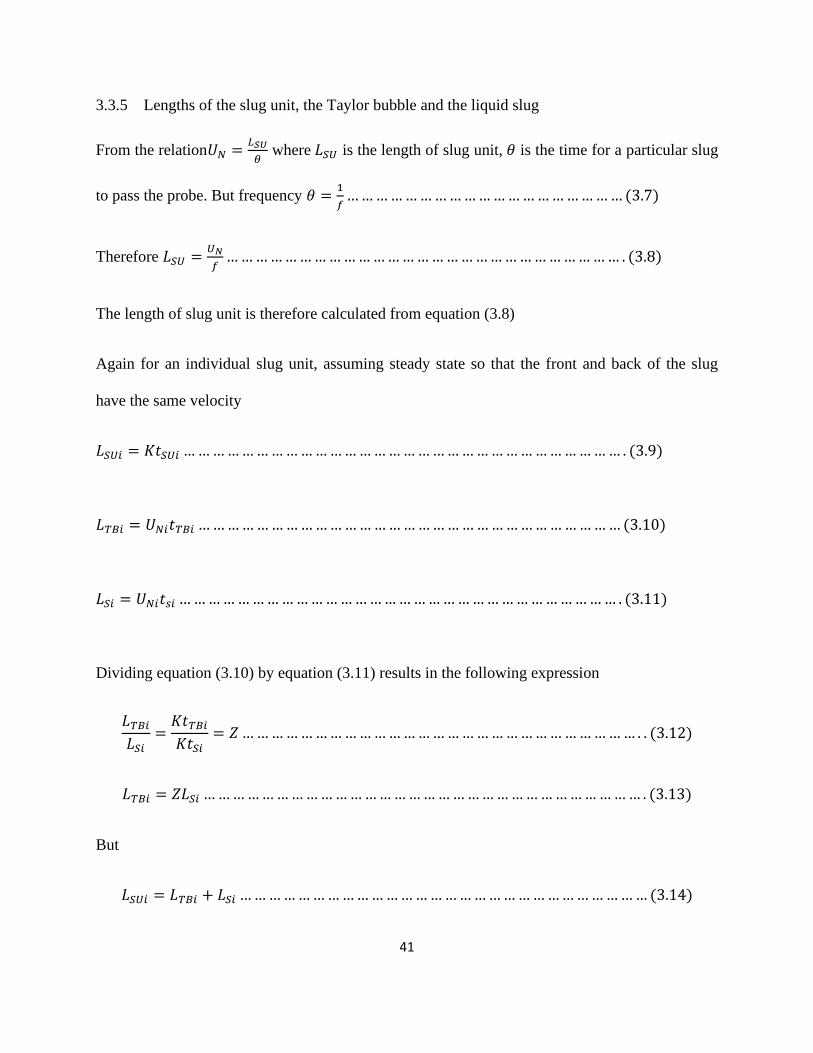
Figure 4.7 a plot of void fractions in the Taylor bubbles against gas superficial velocity for various
liquid superficial velocities ......................................................................................................................... 55
Figure 4.8 a plot of void fractions in the liquid slug against gas superficial velocity for various liquid
superficial velocities ................................................................................................................................... 56
Figure 4.9 Influence of gas superficial velocity on gravitational and frictional pressure gradient ..... 58
Figure 4.10 Influence of gas superficial velocities on the accelerational and total pressure gradient ... 59
Figure 4. 11 Structure velocity for 0o and 30
o inclination angles obtained from experiments using ECT
and empirical correlations of Bendiksen (1984) and Nicklin et al. (1962) correlation ............................... 61
Figure 4.12 (a) and (b)Shoham (2006) flow pattern map for and air/silicone mixture ............... 63
Figure 4.13 PDF for 0o and 30
o pipe inclination .................................................................................... 66
Figure 4.14 Effect of gas superficial velocity and angle of inclination on frequency for various
liquid superficial velocity ........................................................................................................................ 66

xii
LIST OF TABLES
Table 3.1 Physical properties of air/silicon ............................................................................................. 38
Table 4.1 Average root mean square (ARMS) of empirical correlation for the 0o and 30
o pipe
inclination angles…………………………………………………………………………………… 51

1
Chapter 1
1.1 Introduction
The simultaneous flow of several phases which may be a gas, liquid or a solid both in pipes and
porous medium is referred to as multiphase flow. Brennen - (2005) defined multiphase flow as
any fluid flow consisting of more than one phase or component. Multiphase flow has received
both academic and industrial interest over the years because of its importance in nature and
engineering applications.
Liquids transported in containers are subjected to splattering and unpredictable transient loads,
which may affect the integrity of thin-shell containers, or make the transporting vehicle unstable
Aydelott and Devol (1987). Typical practical situations where two-phase gas-liquid flow exists
are in the nuclear, power, chemical and petroleum industries Brennen- (2005). For example, the
calculation of pressure drop is reliant on the two - phase flow dynamics.
Multiphase flow in pipelines is a common occurrence in the petroleum industry Abduvayt
(2003). According to Abduvayt (2003), multiphase flow in pipes which is known to be a
common occurrence in the petroleum industry is usually conveyed through a single pipeline to
storage facility since it is very expensive to separate the produced mixture of oil before
transporting it. Multiphase flow exhibit several flow regimes in conduit depending on the gas
and liquid flow rates and pipe inclination angle. Different inclinations will cause changes in the
flow regime transitions and flow characteristics Kang et al. (1996).Measurement and prediction
of liquid-gas multiphase flow regimes that occur in processing pipelines and wellbores are
crucial to the petroleum industry. The understanding of the flow regimes is vital for engineers to
2
improve the configuration of pipelines and downstream processes to attain economic and safe
design. Hence the ability to predict the multiphase fluid flow behavior of these processes is
central to the efficiency and effectiveness of those processes Beggs (1973).
In the oil production systems, one component which has received much attention is the effect of
pipe inclination on fluid flow, however there has not been enough experimental investigation
using industry related fluids under various process conditions. The prediction of two-phase flow
regimes in greater details with precision requires instrumentation that can measure and describe
the flow within the pipes coupled with the use of more related industrial fluids. . This study seeks
to investigate the effect of changing pipe inclination angle from 0o to 30
o on gas–liquid flow
using electrical capacitance tomography (ECT) data. The interest of this work is towards oil and
gas industry applications.
1.2 Gas-liquid flow in inclined pipes
The multiphase mixture is transported through a single pipeline to a central gathering
station. It is very expensive to separate the produced mixture of oil and gas. During this
transport, several flow regimes occur depending on the gas and liquid flow rates. The
distances the multiphase mixture must be transported are often long and the deviations
from horizontal flow are always present. These changes in inclination cause changes in
the flow regime transitions and flow characteristics, which have a definite effect on the
corrosion rate experienced by these pipelines Kang and Jepson (2002). In offshore
operations very long pipelines are used to reach separation facilities sited at nearby platform or
onshore. Separators, piping components or slug-catchers are used to control flow and processing
during production and transportation of oil and gas, Shoham (2006). The application of

3
multiphase flows in the transportation of oil and gas through flow lines may be cost-effective for
reservoir development. But, the hurdle to overcome is how to develop multiphase technology to
transport oil and gas from subsea production units to processing facilities at nearby plat forms or
onshore separating facilities Zoeteweij (2007).
The transportation of gas and liquid in conduits can lead to several topological configurations
called flow patterns or flow regimes. This flow regime is usually observed when gas and
liquid flow rates are sufficiently high. The simultaneous presence of gas and liquid in a
pipe requires a more complex method of analysis than that applied to single phase flow
problems. The composition variation of fluids inside this subsea flow line network can cause
operational problems, such as non-continuous production or shut-down to damage equipment
Beggs (1973).
Simultaneous production of gas-water and or oil-water mixtures may result in multiphase flow
conditions in the flow line systems which connect the source to the production platform. As the
production of the field progresses, the water content of the produced multiphase mixture
increases to cause different mixture compositions, which affect the flow pattern and flow
behavior Hernandez-Perez (2008).
As oil and gas reserves are being depleted in developed areas, activity is shifting to harsher and
less accessible environments. This requires simultaneous transport of produced fluids to a land-
based separation facility, with only minimal treatment offshore for such undesirable effects as
corrosion, wax and hydrates Zheng et al. (1992).

4
Both the onshore and offshore cases can result in the simultaneous transport of oil and gas over
long distances which require pipes which may be deviated from the horizontal Zheng et al.,
(1992). The accurate prediction of multiphase flow characteristics in these flow lines is required
for the design, as well as the economical and safe operation of these transportation systems. Flow
patterns are also dependent on the elevation profile of the pipeline Scott et al., (1990).For
instance, flow patterns encountered in steeply inclined pipelines are different from those found in
horizontal and near horizontal pipelines. The proper design of multiphase pipelines, together
with downstream processing facilities, requires a thorough understanding of the behavior of
multiphase flow in pipelines. As part of the scope of this study, this work seeks to evaluate the
effects of pipe inclination and characterizing slug in pipes.
1.3 Problem statement
Pipes that make up oil and gas wells are not vertical but could be inclined at any angle
between the horizontal and the vertical which is a significant technology of modern drilling
Zheng et al., (1992). Although extensive research in two-phase flow has been conducted during
the last decades but most of this research has concentrated on either horizontal or vertical flow.
Several good correlations exist for predicting pressure drop and liquid holdup in either horizontal
or vertical flow, but these correlations have not been successful when applied to inclined flow.
Moreover many gathering lines and long-distance pipelines in the petroleum industry pass-
through areas of hilly terrain therefore, in order to predict pressure drop, the liquid holdup must
be accurately predicted Singh et al. (1970).

5
The ability to predict liquid holdup also is essential for designing field processing equipment,
such as gas liquid separators. Hence, in order to accomplish a reliable design of gas-liquid
systems such as pipe lines, boilers and condensers, a prior knowledge of the flow pattern is
needed.
1.4 Aim and Objectives
The aim of this research is to investigate the effect of pipe inclination on void fraction
distribution. In order to achieve the aim the following objectives will be met
1.) To analyze raw experimental ECT data obtained from an experimental investigation
carried out by Abdulkadir, (2011) using air-silicone oil mixture in a 67 mm diameter
pipe inclined at 0o and from the horizontal.
2.) To characterize the hydrodynamics of slug flow both in the and pipe
inclination via the determination of the following: the translational velocity, void
fraction in the liquid slug, void fraction in Taylor bubble, length of liquid slug and
Taylor bubble, the frequency of slugging and the pressure drop.
1.5 Structure of the thesis
The layout of this thesis is summarized as follows;
Chapter 1-Introduction- This Chapter provides an introduction to the thesis, defining the
problem, aim and objectives of the study, methodology and the structure of the thesis.
Chapter 2-Literature Review - This chapter is concerned with review of published work on void
fraction distribution in pipes. Flow pattern transition, maps and identification in vertical,
horizontal and inclined pipes for two-phase flow was reviewed followed by void fraction

6
concept and correlations for inclined pipes. A pressure drop correlation for upward inclined two-
phase flows was also reviewed.
Chapter 3-Data Acquisition Setup - This chapter describes the experimental facility that was
used to measure the time varying liquid holdup for this work.
Chapter 4-Results and Discussion- This chapter looks at the results obtained from the
experimental flow facility and critical analysis of the results to achieve the objectives stated.
Chapter 5 - Conclusions and recommendations - This chapter brings together all the key
conclusions from this work and provides some recommendations.

7
Chapter 2
LITERATURE REVIEW
Two-phase gas-liquid flow is a common phenomenon in nuclear reactors, chemical reactors,
power generation, process industries and petroleum industries Abduvayt (2003). In multi-phase
flow studies, gas-liquid flows are the most studied compared to other types of flow. The behavior
of two-phase gas-liquid flow compared to a single phase flow of either a gas or liquid is
significantly different. In order to predict and control two-phase flow behavior and its
corresponding pressure drop, heat transfer and mass transfer characteristics, a good
understanding of the hydrodynamics of the system is required. This chapter deals with the
fundamentals of two-phase gas-liquid flows with emphasis on pipe inclination. It will also
discuss flow pattern maps and the methods of their identification
2.1 Gas-liquid flow in inclined pipes
The study of two-phase gas- liquid flow in inclined pipes for the last few decades are
summarized below, it outlines the experiment conducted and the parameters involved. Two-
phase gas–liquid flow was investigated in theoretical and experimental studies. Most data
reported on flow pattern transitions have dealt with either horizontal or vertical tubes with only
limited results reported for inclined pipes.
Sevigny (1962) conducted a comprehensive study of two-phase flow in inclined pipes. Air and
water were the test fluids in 20 mm ID pipe with varying pipe inclinations. He found that
pressure gradients are greatly affected by inclination angles.
Zukoski (1966) studied the effect of pipe inclination angle on bubble rise velocity in a stagnant
liquid. He concluded that, depending on the pipe diameter, surface tension and viscosity of fluids

8
may appreciably affect the bubble rise velocity. His findings also showed that for some
conditions an inclination angle as small as from the horizontal can cause the bubble rise
velocity to be more than 1.5 times the value obtained for horizontal pipes.
A study of slug flow in inclined pipes was reported by Singh and Griffith (1970). They measured
pressure drop and liquid holdup in pipe with diameters of 0.626, 0.822, 1.063, 1.368, and 1.600
in. (16-40 -mm), at inclination angles of plus and minus 10° and 5o from horizontal, and at 0°.
Liquid holdup was found to be independent of inclination angle.
Bonnecaze et al. (1971) developed a model for two phase flow in inclined pipeline and claimed
that pressure drop was a strong function of the liquid holdup in the slug unit.
Later, Beggs (1972) used a 50.8 and 62.9 mm ID pipe and carried out a study of inclination
effects. He experimentally showed that liquid holdup was strongly affected by pipe inclination
angle.
Mattar and Gregory (1974) conducted experiments to find the effect of inclination on slug
velocity, holdup and pressure gradient. They found that for uphill pipe sections, slug flow was
the predominant flow pattern, and for downhill pipe sections stratified flow dominated. They
also observed that hydrostatic head for slug flow dictated pressure gradient in uphill sections.
Gould et al. (1974) published flow pattern maps for horizontal and vertical flow and for up-flow
at inclinations.
Later, Spedding and Chen (1981) experimentally studied pressure drop in two phase flow in
inclined pipe corroborating the relationship between flow pattern and pressure drop.
In 1985, Barnea et al examined the effect of the inclination angle on the flow pattern transition
boundaries by varying the inclination angle in small steps in the range of . They found
that small changes in the angle of inclination from the horizontal can have profound effects on

9
the flow patterns that exist. At very small inclination angles, the force of gravity acting in the
flow direction can be of the order of the wall shear stress. On the other hand, small deviations
from the vertical have little effect on flow patterns.
Kokal and Stanislav (1989) showed that the uphill-flow regimes were found to be similar to
the horizontal-flow regimes except that very limited stratified flow was observed for uphill
flows. The downhill-flow regimes on the other hand were found to be very different and more
complex.
Xiao et al. (1990) developed a comprehensive mechanistic model for gas-liquid two-phase flow
in horizontal and near-horizontal pipelines. The comprehensive mechanistic model incorporated
flow pattern prediction capabilities. Separate models could then be used to calculate different
flow characteristics like liquid holdup and pressure gradients. The model was validated with a
comprehensive databank.
Roumazeilles et al. (1994) performed an experiment on downward simultaneous flow of gas and
liquid in hilly terrain pipelines and injection wells. They developed most of the methods for
predicting pressure drop in gas-liquid two phase flow in pipes for either upward vertical or
upward inclined pipe. They investigated experimentally downward concurrent slug flow in
inclined pipe via obtaining liquid holdup and pressure drop measurements for downward
inclination angles from at different flow condition.
Cook and Behnia (2000) presented a comprehensive treatment of all sources of pressure drop
within intermittent gas-liquid flows. Calculated pressure loss associate with the viscous
dissipation within a slug, and the presence of dispersed bubbles in a slug were accounted for,
without recourse to the widely used assumption of homogenous flow. The results show that

10
existing intermittent flow models predict pressure gradients considerably lower than were
observed.
Colmenares et al. (2001) studied pressure drop models for horizontal slug flow for viscous oils.
Their experimental results suggested that the slug flow region in the flow pattern map was
enlarged when the oil viscosity increased. Experimental results from a 0.48 Pas viscous liquid-
gas two-phase flow also concluded that as liquid viscosity increased, slug frequency and liquid
film holdup increased while the slug length decreased.
Lewis, et al. (2002) discussed utility of the hot-film anemometry technique in describing the
internal flow structure of a horizontal slug flow pattern within the scope of intermittent nature of
slug flow. It was shown that a single probe can be used for identifying the gas and liquid
phases and for differentiating the large elongated bubble group from the small bubbles present
in the liquid slug.
Zhang et al.(2003) developed a unified hydrodynamic model to predict flow pattern transitions,
pressure gradient, liquid holdup and slug characteristics in gas-liquid pipe flows for all
inclination angles (from from horizontal).
Gokcal (2005) experimentally studied the effects of high viscosity liquids on two-phase oil-gas
flow. He observed a marked difference between the experimental results and the model
predictions. Intermittent slug and elongated bubble flow were the dominant flow pattern.
Later, Ribeiro, et al. (2006) compared new data on pressure drop and liquid hold-up obtained in a
horizontal square cross-section channel against several existing correlations and models for gas
liquid flow. The hold-up data were taken for conditions of wavy stratified and pseudo-slug flow.
Pressure drop results were only obtained for wavy stratified flow.

11
Wongwises and Pipathattakul (2006) studied experimentally two phase flow pattern, pressure
drop and void fraction in horizontal and inclined upward air–water two-phase flow in a mini-gap
annular channel. They observed and recorded the flow phenomena, which are plug flow, slug
flow, annular flow, annular/slug flow, bubbly/plug flow, bubbly/slug–plug flow, churn flow,
dispersed bubbly flow and slug/bubbly flow by high-speed camera. Also a slug flow pattern was
found only in the horizontal channel while slug/bubbly flow patterns are only in inclined
channels. When the inclination angle was increased the onset of transition from the plug flow
region to the slug flow region (for the horizontal channel) and from the plug flow region to
slug/bubbly flow region (for inclined channels) shift to a lower value of superficial air velocity.
Gokcal (2008) later conducted an experimental study to develop closure relationships for two-
phase slug flow characteristics for high viscosity oils. The parameters that he considered include
pressure gradient, drift velocity, translational velocity, slug length and slug frequency. All tests
were conducted for horizontal flow and oil viscosities range from 0.181 Pas to 0.585 Pas.
Hernandez-Perez et al. (2010) studied the effect of pipe inclination on the internal structure of a
liquid slug body at different pipe inclination angle from the horizontal to vertical. The
working fluid employed in the experiment was air and water with a pipe diameter of 67 mm
using WMS to take measurements. The superficial gas and liquid velocity are
and , respectively. However, it was revealed in their work that void fraction distribution
was strongly affected by pipe inclination, but does not strongly affect the bubble size distribution
and they finally concluded that there exist a relationship between void fraction and
bubble size distribution in a liquid slug body.
Arvoh et al.(2012) used a combination of gamma measurements and multivariate calibration
to estimate multiphase flow mixture density and to identify flow regime. The experiments were

12
conducted using recombined hydrocarbon. These were conducted at a temperature of and a
75-bar pressure. Two angles of inclination (1o and 5
o) and two water cuts (15% and 85%) were
investigated. The estimated mixture densities were accurate as compared with those from the
single-energy gamma densitometer with a root mean square error of prediction of 13.6
and
for 1o angle of inclination and 17 and
for 5o pipe inclination. Flow patterns
observed in upward inclined flow are quite similar to those observed in vertical upward
flow, especially for near-vertical systems. They include bubbly and dispersed bubbly, slug,
churn and annular flow in inclined systems.
Esam and Riydh (2013) studied flow pattern and pressure drop of gas–liquid flow in inclined
pipe experimentally. The diameter of test section is 50 mm, and overall length of 4 m. The
inclination angle of the test section is 30o. Air and water are used as working fluids. The
experimental results showed that the inclination angle has a significant effect on the flow pattern
transition and pressure drop. It was noted that the pressure decreases with distance along pipe
when gas superficial velocity increased and also increased liquid superficial velocity. And the
slug liquid appears when the fluctuation in pressure accrues. The liquid holdup decreased when
increased gas superficial velocity and depends on the flow pattern.
2.2 Flow regime classification
The variation in physical distribution of fluid phases during multiphase flow through conduits or
pipes is called flow regime (flow pattern). Numerous investigations have been carried out in
identifying flow regimes and the transitions between them. Detailed reviews of earlier work
which focuses on two phase flow patterns and pattern transition have been published by Govier
and Aziz (1972), Hewitt (1982) and Delhaye et al. (1981). Recent experimental and semi
theoretical studies reviews have been provided by Thomas and Collier (1994). In the

13
simultaneous flow of two-phases in pipes, the fluids tend to exhibit a number of different flow
regimes. The flow regime exhibited is dependent on the relative magnitude of flow rate, pipe
diameter, pipe inclination angle and fluid properties (density and viscosity). In wellbores several
different flow regime can exist due to the large pressure and temperature changes encountered
during upward flow of fluids Mukherjee et al. (1999). Knowledge of the flow pattern is vital to
define fluid mechanics in multiphase flow and also for successful operation in oil production
from older subsea oil wells. Usually flow regimes are grouped under horizontal, vertical, and
inclined pipes orientation. According to Legius (1997), multiphase flow in vertical pipes,
exhibits; bubbly, slug, churn or annular flow patterns and in horizontal and in - inclined pipes,
these flow patterns are extended to include smooth stratified, stratified wavy and plug flows.
2.2.1 Vertical flow regimes
In two-phase gas-liquid flow in pipes or channels, an interface exists between the phases. The
phase boundary can take a variety of configurations, known as the flow pattern. The existing
flow pattern in a given two-phase flow system depends on the operational parameters (gas and
liquid flow rates), the geometrical variables (pipe diameter and pipe inclination angle), and the
physical properties of both phases (gas and liquid densities, viscosities and surface tension)
Elekwachi (2008). According to Beggs and Brill (1994), they described the four flow observed in
gas-liquid flow in vertical pipe as bubble flow, slug flow, transition (annular-slug transition)
flow and mist (annular-mist) flow. For upward multiphase flow of gas and liquid, the most
described by Taitel et al. (1980) are namely- bubble flows, slug flow, churn flow and annular
flow. These flow patterns, shown in Figure 2.1, are described in order of increasing gas flow
rate.

14
Figure 2.1 -Upward vertical flow pattern- Taitel et al. (1980)
2.2.1.1 Bubble flow pattern- In the bubble flow pattern, the liquid phase almost
completely fills the pipe and the gas is present in the liquid as small bubbles and is randomly
distributed. The diameters of the bubbles vary randomly. At high gas flow rate, the number of
bubbles in solution increases resulting in frequent collisions between the bubbles. This causes
more bubbles to coalesce. Griffith and Wallis (1961) noted that the bubble/slug transition occurs
at a void fraction of about 0.25 - 0.30.
2.2.1.2 Slug flow pattern- The gas phase is more dominant in the slug flow although
liquid phase is still continuous. The gas bubbles merge with each other to form stable bubbles of
almost equal shape and size which are approximately the same diameter of the pipe. These

15
bubbles formed are called Taylor bubbles. Slug flow consists of successive Taylor bubbles and
liquid slug which link the entire pipe cross section. In between the Taylor bubbles and the pipe
wall there exist a thin liquid film, these film enters into the following liquid slug and produce a
mixing zone aerated by small gas bubbles Taylor et al. (1950)-According to Jayanti and Hewitt
(1992), four major theories have been proposed to explain the transition from slug flow to churn
flow in vertical pipes. These mechanisms are entrance effect, flooding, wake effect and bubble
coalescence mechanisms.
2.2.1.3 Churn flow pattern- Churn flow is chaotic flow of gas and liquid also referred to
as froth flow and semi-annular flow is a highly disturbed flow of gas and liquid in which both the
shape of the Taylor bubble and liquid slug are distorted by increase in the gas velocity which
causes the liquid slug to become unstable, leading to its break-up and fall. This liquid merges
with the approaching slug, which then resumes its upward motion until it becomes unstable and
falls again. The alternating direction of motion in the liquid phase in irregular manner is typical
of churn flow, Brill and Mukherjee (1999).
2.2.1.4 Annular flow pattern- Annular flow is also referred to as mist or annular-mist
flow Duns and Ros (1963) and Aziz and Govier (1972). It is characterized by a central core of
fast flowing gas and a slower moving liquid film that travels around the pipe wall. The shearing
action of the gas at the gas-liquid interface generates small amplitude waves (ripples) on the
liquid surface. By increasing the flow conditions beyond critical gas and liquid flow rates, large
amplitude surges or disturbance waves occur.

16
Figure 2.2 Vertical flow patterns Abbas (2010)
2.2.2 Horizontal flow regimes
Two phase flow patterns in horizontal tubes are similar to those in vertical flows but the
distribution of the liquid is influenced by gravity that acts to ensure the liquid is confined at the
bottom of the tube and the gas at the top. Flow patterns for co-current flow of gas and liquid in a
horizontal pipe are characterized as follows Taitel (2000)
2.2.2.1 Bubbly flow- The gas bubbles are dispersed in the liquid with a high
concentration of bubbles in the upper half of the pipe due to their buoyancy. When shear forces
are dominant, the bubbles tend to disperse uniformly in the pipe. In horizontal flows, the regime
typically only occurs at high mass flow rates Loilier (2006).
2.2.2.2 Stratified flow- At low liquid and gas velocities, complete separation of the two
phases occurs. The gas goes to the top and the liquid to the bottom of the tube, separated by an

17
undisturbed horizontal interface. Hence, the liquid and gas are fully stratified in this regime
Loilier (2006).
2.2.2.3 Stratified-wavy flow- Further increasing the gas velocity, these interfacial waves
become large enough to wash the top of the tube. This regime is characterized by large
amplitude waves intermittently washing the top of the tube with smaller amplitude waves in
between. Large amplitude waves often contain entrained bubbles. The top wall is nearly
continuously wetted by the large amplitude waves and the thin liquid films left behind Loilier
(2006).
2.2.2.4 Plug flow- This flow regime has liquid plugs that are separated by elongated gas
bubbles. The diameters of the elongated gas bubbles are smaller than the tube, such that, the
liquid phase is continuous along the bottom of the tube below the elongated bubbles. Plug flow is
also sometimes referred to as elongated bubble flow Taitel (2000).
2.2.2.5 Slug flow- At higher gas velocities, the diameters of elongated bubbles become
similar in size to the channel height. The liquid slug separating such elongated bubbles can also
be described as large amplitude waves Taitel (2000).
2.2.2.6 Annular flow- At even larger gas rates, the liquid forms a continuous annular film
around the perimeter of the tube, similar to that in vertical flow but the liquid film is thicker at
the bottom than the top. The interface between the liquid annulus and the vapor core is
distributed by small amplitude waves and droplets may be dispersed in the gas core. At high gas
fractions, the top of the tube with its thinner film becomes dry first, so that the annular film
covers only part of the tube perimeter and thus this is then classified as stratified-wavy flow
Taitel (2000).

18
2.2.2.7 Mist flow- Similar to vertical flow, at very high gas velocities, all the liquid may
be stripped from the wall and entrained as small droplets in the continuous gas phase (Thome,
2007). Taitel (2000) represents the different co-current flow regimes of gas and liquid that can be
encountered in a horizontal pipeline
Figure 2.3 Flow- patterns- in- horizontal- gas-liquid -flows- Taitel (2000)
2.2.3 Flow pattern maps
A flow pattern map is a representation of the existence of flow patterns in a two dimensional
domain in terms of system variables. They consist of flow regimes separated by transition lines
and are gotten from the description and classification of the various flow patterns Omebere-Iyari
(2006). The flow pattern that can be observed is dependent on- the fluid properties, flow rates,

19
pipe diameter, pipe inclination angle, and operating conditions at ends of the pipe. The accurate
prediction of the flow pattern existing under a given conditions is required, since every flow
pattern has a unique hydrodynamic characteristics.
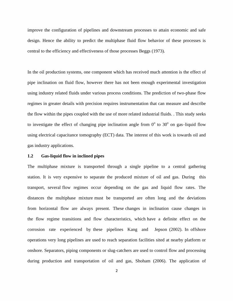
2.2.3.1 Baker flow pattern map
The first to recognize the importance of the flow pattern as a starting point for the calculation of
pressure drop, void fraction, and heat and mass transfer was Baker (1954). He published the
earliest flow pattern map for horizontal flow, presented below. To utilize this map, first the mass
velocities of the liquid -and vapor -must be determined. Then the gas-phase parameter λ
and the liquid-phase parameter ψ are calculated as follows:
(
)
(
) [(
) (
)
]
20
Figure 2.4 Baker (1954) flow pattern map for horizontal flow in a tube
Where , , and σ are the properties of the fluid and , , and are
the reference properties of air and water at standard atmospheric pressure and room temperature.
The map shown in Figure 2.4 was developed based on air - water data. and ψ are standard
dimensionless parameters that should take into account the variation in the properties of the
fluid.
2.2.4 Flow pattern identification
Gas-liquid flow pattern can be identified by observing visually the flow in transparent pipes. But
this has its own limitations and cannot be done all the time because; high gas and liquid flow
rates will make visual observation impossible. Hence high speed photography is often used. The
above two methods are not applicable in the industries because, actual industrial pipes are not

21
transparent, Hernandez-Perez (2008). Hubbard and Dukler (1966) also developed a method for
flow regime determination, which employs spectral analysis to study the observed pressure
fluctuations. The technique is based on the idea that, the gas-liquid flow patterns are
characterized by fluctuations in wall pressure. The power spectral density (PSD) of digitized
time response, gotten from a pressure transducer located flush to the wall of the flow pipe was
calculated from autocorrelation method. Three types of power spectral distributions were
obtained and used to group the various flow regimes measured for horizontal air-water pipe
flows. These are shown in Figure 2.5, namely- (a) separated flows; containing a peak at zero
frequency; this type of response is obtained from stratified and wavy flows, (b) dispersed flows;
possessing a flat and relatively uniform spectrum and (c) intermittent flows; with a characteristic
peak; this is obtained for plug and slug flows.
Figure 2.5 a, b, c Flow identification by power spectrum density of pressure gradient
Hubbard and Dukler (1966). Adapted from Hewitt (1978)
This was the first effort to categorize flow patterns centered on proofs and was monitored by the
studies carried out by Nishikawa et al. (1969) and Kutataledze (1972). Investigations by Tutu
(1982) and Matsui (1984), analyzed the time variation of pressure gradient and pressure
fluctuations, respectively. Tutu (1982) used the probability density distribution to identify the

22
flow patterns observed in vertical flow systems. But, Keska and Williams (1999) established that
the pressure system Tutu investigated did not offer a better flow pattern recognition method
relative to capacitive and resistive systems. Vince and Lahey (1982) obtained a series of chordal-
averaged void fraction measurements using a dual beam x-ray system for low pressure air-water
flow in a vertical pipe. Their results were used to generate corresponding PDF and PSD
functions of the recorded signals. They observed that the calculated moments were responsive to
the velocity of the liquid phase. Jones and Zuber (1975) advocated the use of the photon
attenuation technique, to measure the time-varying, cross-sectional averaged void fraction. This
system used a dual x-ray beam device for a two-phase mixture of air and water, flowing
vertically. It was observed that the probability density function (PDF) of the void fraction
fluctuations shown in Figure 2.6 could be used as an objective and measurable flow pattern
discriminator.
Figure 2.6 Flow pattern identification by probability distribution function of void
fraction Jones and Zuber (1975)
Costigan and Whalley (1997) upgraded the PDF methodology of Jones and Zuber using
segmented impedance electrodes and successfully grouped flow patterns into six: discrete
bubble, spherical cap bubble, stable slug, unstable slug, churn and annular. Figure 2.6(a) to 2.6(f)

23
shows the Void fraction traces and corresponding PDFs of the six flow patterns respectively,
from Costigan and Whalley (1997):
Figure 2.6 (a) a single peak at low void fraction is indicative of discrete bubble flow
Figure 2.6 (b) a single peak at low void fraction accompanied by a long tail is indicative
spherical cap bubble.

24
Figure 2.6 (c) a double peak feature with the higher peak at low void fraction and the
lower peak at a higher void fraction signifies stable slug flow
Figure 2.6 (d) a double peak feature with the lower peak at low void fraction and the
higher peak at a higher void fraction signifies unstable slug flow

25
Figure 2.6 (e) a single peak at a high void fraction with a broadening tail is indicative of
churn flow
Figure 2.6 (f) a single high peak at high void fraction is defined as annular flow
2.3 Tomographic techniques
Tomography is a non-invasive imaging technique allowing for visualization of the internal
structure by the use of any kind of penetrating wave. Alternatively, the term tomography usually
refers to a- technique that enables the determination of the density distributions in a cross-section
of an object. A tomograph is a device used in tomography, while the-image produced is a
tomogram. The two types of tomographic techniques are intrusive and non-intrusive. Shemer et

26
al. (2006) describes the later method as it uses either a set of radiation attenuation
measurements such as x-ray, γ-ray, sound waves or impedance measurements among various
pairs of electrodes glued flush to the pipe surface. Kumar et al.(1995) used a computed
tomographic scanner using γ-ray for measuring void fraction distribution in two phase flow
system such as fluidized beds and bubble columns. Creutz and Mewes (1998) also employed
an electro-resistance tomography to measure the concentration distribution inside a gas-liquid
centrifugal pump. In addition, an x-ray tube and scintillating detectors were used by Kendoush
and Sarkis (2002) for void fraction measurements.
In this thesis work, liquid hold up data obtained by Abdulkadir (2011) using an advanced non-
intrusive tomographic measuring instrument called electrical capacitance tomography (ECT) was
employed.
2.4 Void fraction
The fraction of the channel volume that is occupied by the gas phase is described as void
fraction. The void fraction (ε) is one of the most important parameters used to characterize two-
phase flows. Void fraction could be measured by many methods such as quick-close valve, γ
rays, x-rays, microwave, etc. ECT technology is prospectively useful because it is accurate,
economical, non-intrusive, safe and fast. ECT is a kind of tomography process technology and
provides a new way to solve the problems of void fraction measurement Li (2001).
However, it is a significant physical value for determining other numerous parameters such as
two-phase flow viscosity and density. Void fraction data is also used for obtaining the relative
average velocity of two-phases and also employed in models for predicting flow
pattern transitions, heat transfer, interfacial area calculation and determination of pressure
drop. In addition, literature reported various correlations for predicting void fraction and

27
classified them in terms of their method and physics involved in deriving these correlations as
flow dependent or flow independent.
2.4.1 Concept of void fraction
Void fraction is defined as the volume of space the gas phase occupies in a given two phase flow
in a pipe- It is a key parameter which is used in estimating other parameters such as
pressure drop, liquid holdup and heat transfer. In facilitating better understanding of void
fraction, it is worthwhile to highlight some of the most common terminologies and definitions of
parameters that would be encountered throughout this work. For a total pipe cross sectional
area ; the void fraction is given by
Liquid holdup is the complement of the void fraction in the pipe; it is the remaining volume of
space occupied by the liquid phase. Thus, liquid holdup is
The quality of the mixture, , in the isothermal flow case we are considering here is taken as the
input mass of the gaseous phase to that of the total mixture mass of m, hence
The slip ratio, , is defined as the ratio of the actual velocities between the phases. A slip ratio of
unity for a mixture being the homogeneous case where it is assumed that both phases travel at
the same velocity. The slip ratio is defined as

28
The superficial gas , and liquid , velocities are defined as the velocities of the gas or
liquid phase in the pipe assuming the flow is a single phase in either gas or liquid respectively.
From the definitions given above and writing conservation of mass for each phase and total flow,
we can define the relationships,
(
) (
)
2.4.2 Classification of void fraction
At a given point in the flow, the local fluid is either gas or one of the other phases. The
probability of finding gas at a given point may be determined using local probes and is referred
to as the local void fraction - Hewitt et.al (1982).Thus means when liquid is
present and when gas is present. Typically, the local time averaged void fraction
cited, or measured using a miniature probe, which represents the fraction of time gas, was
present at that location in the two-phase flow. If represents the local instantaneous
presence of gas or not at some radius r from the channel at time t, then when gas is
present and when liquid is present. Thus, the local time-averaged void fraction is
defined as
∫
The chordal void fraction is typically measured by shinning a narrow radioactive beam
through a channel with a two phase flow inside, calibrating its different absorptions by the vapor

29
and liquid phases, and then measuring the intensity of the beam on the opposite side, from which
the fractional length of the path through the channel occupied by the vapor phase can be
determined. The chordal void fraction is defined as
Where is the length of the line through the gas phase and is the length through the liquid
phase” Thome (2004).
The cross- sectional void fraction is typically measured using either an optical means or by
an indirect approach, such as the electrical capacitance of a conducting liquid phase. Also, it is
the most widely used void fraction definition known as cross-sectional average void
fraction which is based on the relative cross-sectional areas occupied by the respective phases.
The cross-sectional void fraction is defined as
Where -is the area of the cross-section occupied by the vapor phase and -is that of the
liquid -Thome (2004).
Another measure is the volume-averaged void fraction. This can be interpreted as the fraction of
volume of the reference volume occupied by the gas phase at time (t). The volumetric void
fraction - is typically measured using a pair of quick-closing valves installed along a
channel to trap the two-phase fluid, whose respective gas and liquid volumes are then
determined. The volumetric void fraction can be represented as

30
Quality (x) of a two-phase flow is defined as the ratio of the gas mass flow rate to the total mass
flow rate but sometimes confused with void fraction definition. The quality is expressed in terms
of mass and is a function of the phase density and void fraction. The quality (x) is given by
“However, another important definition in two -phase flow also confused with void fraction is
the gas volumetric flow fraction denoted as β. It refers to the ratio of the gas volumetric flow rate
over the mixture volumetric flow rate given by
Where - and – are the volumetric flow rates of liquid and gas respectively.
The major difference between void fraction and gas volumetric flow fraction is that, in void
fraction, there is slippage in two- phase flow due to density difference whiles the later assumes
that both phases move with the same velocity and hence known as void fraction in the
homogeneous flow” Thome (2004).
2.4.3 The measurement principle
Void fraction can be measured by measuring the changes of material properties owing to the
presence or absence of the gas. Some of the properties that can be used for checking the presence
of gas and the corresponding sensors are as follows:
Electrical impedance
Impedance probe
Refractive index
Optical probes

31
Density-(absorption coefficient)
X-rays or gamma ray densitometers
2.5 Void fraction correlations for inclined pipes
The majority of the correlations developed for void fraction are for horizontal with very few for
other inclination angles, the common one being upward. Categorizing the correlations along their
applicability with regard to angle of inclination would not serve any purpose as most of them
would fall under the horizontal case. Most of the data from which the correlations have been
developed were from small pipe diameters, short length pipes in a laboratory setting with
controlled, and relatively small mass flow rates while mixtures of air-water dominate with regard
to the fluids considered Woldesemayat et al. (2007).
The correlation of Guzhov et al. (1967) which can handle the plug and stratified flow regimes in
pipes with small inclination angles to the horizontal (±9o) is also considered here. The correlation
is a function of the homogeneous void fraction and the mixture Froude number.
( ( ))
Greskovich and Cooper (1975) developed a correlation from air- water data for inclined flows. It
was noted that the data showed little diameter dependency above 2.54-cm but was considerably
dependent on inclination angles.
[ (
)]

32
A general type of correlation given in a plot format by Flanigan-(1958) put into equation form
by the AGA (American Gas Association) is considered. The correlation assumes that pipe
inclination has no effect on void fraction and that it is only a function of gas superficial velocity.
Gomez et al.(2000) developed a correlation for predicting liquid holdup for slug flow for
horizontal, inclined and vertical orientations. The data covers pipe diameters between 5.1 – 20.3
inches and the fluids considered were air, nitrogen, freon, water and kerosene. The liquid slug is
seen to be dependent on the inclination angle, mixture velocity and viscosity of the liquid phase.
They claimed surface tension has no significant effect on the holdup in comparison to the
viscosity of the liquid. The equation is of the form
( )
2.6 Drift flux correlations
This type of correlations are based on the work of Zuber and Findlay (1965) where the void
fraction can be predicted taking into consideration the non-uniformity in flows and the difference
in velocity between the two phases. This model is good for any flow regime. It has the general
expression given by
)
Where- is the distribution parameter and is the drift velocity.
Kokal and Stanislav-(1989) correlated their air-oil experimental data in horizontal and near
horizontal (±9o) pipe using the drift flux relation and recommended their correlation for all flow
regimes. It is given as
[
]

33
2.7 Pressure drop in two-phase inclined pipes
The ultimate goal in two-phase flow models is to calculate the total pressure drop that occurs in a
two-phase flow system. The knowledge of pressure drop in a two-phase flow system is important
for its design. It enables the designer to size the pump required for the operation of the flow
system. The total pressure drop calculations along horizontal pipe consist of two components-
the acceleration pressure drop in the mixing zone and the frictional pressure drop in the slug
body.
In this work, the modified Beggs and Brill correlation stated below is used to calculate the
pressure drop along the entire 6 meters pipe using experimental data - The general pressure drop
equation is given as
( )
Where is a conversion factor to oil field unit
Whilst the new definition of the two-phase friction factor by Beggs and Brill (1957) is given by
the following expression
√ [
(
(
)
)]
Where is the surface roughness, is the mixture Reynolds number which can be
calculated using the following relation.
As mostly stated in literature, mixture density and mixture viscosity are

34
After the calculation of the necessary parameters, the gravitational, frictional and accelerational
pressure drops are calculated from which representative results in the form of graphs are
presented in chapter four.

35
Chapter 3
DATA ACQUISITION SETUP
This chapter presents a summary of the data obtained from a series two-phase air-silicone oil
flow experiment carried out on an inclinable rig by Abdulkadir (2011) at the L3 Laboratories of
the department of chemical and environmental engineering at the University of Nottingham. An
overview of the experimental facility, test fluids and capability of the flow facility presented.
3.1 Overview of the experimental facility
The experimental work was carried out on an inclinable pipe flow rig as shown in figure 3.1 and
3.2. The details of the experiment can be found in Abdulkadir (2011). Data collected from the
experiments was done at laboratory temperature of and 1 bar of atmospheric
pressure with the physical properties of the working fluids shown in table 3.1.

36
Figure 3. 1 The components of the rig (a) liquid pump (b) liquid tank (c) air-silicone oil
mixing section (d) rotameters and (e) cyclone separator Abdulkadir (2011)

37
Figure 3.2 Experimental flow facility Abdulkadir (2011b)
3.2 System (test fluid)
The air-silicone oil system was selected for the reasons listed below (Abdulkadir, 2011b)
It is not toxic, hence environmentally friendly, and reasonably less expensive.
It has thermal stability and transfer qualities - at both hot and cold extremes
It is fire resistant
It has good electrical insulation property
It has no; odour, taste or chemical transference
It is easily detected in acrylic pipe
There are several proven techniques for its use and advanced instrumentation for liquid
holdup or void fraction measurements.

38
Table 3.1 Physical properties of air/silicon
Fluid
Viscosity
(kgm-1
s-1
)
Density
(Kgm-3
)
Surface Tension
(Nm-1)
Thermal Conductivity
(Wm-1
K-1
)
Air 0.000018 1.18
0.02
0.1 Silicone Oil 0.00525 900
Abdulkadir (2011b)
3.3 Parameters determined for this present study
In this present work the method of determination of characterization parameters presented by
Abdulkadir et al. (2014) is adopted. With the ECT data the following parameters were calculated
Lengths of Taylor bubbles and liquid slugs
Slug frequencies,
The velocities of Taylor bubbles and liquid slugs
Void fractions within the Taylor bubbles and liquid slugs
3.3.1 Translational or rise velocity of Taylor bubble (structure velocity)
Fundamentally translational velocity is given by
Where the distance between the two ECT planes and time taken for the individual
slugs to travel between the two planes.

39
3.3.2 Determination of the distance (∆L) between the two ECT planes
The planes are located at 4.4 m and 4.489 m above the mixer section at the base of the riser.
3.3.3 Determination of time delay
As the individual slugs pass between the two ECT planes as shown in figure 3.3, the time taken
to reach the planes are recorded in the form of time series wave output signals. Cross correlating
between these two signals gives the time delay a slug travels between the planes. Cross
correlation for two linearly dependent time series, a and b is the average product of, aa and
bb . Where a and b are the mean of time series a, and b respectively. This average product
is the co-variance of a and b in the limit as the sample approaches infinity. Hence for any time
delay τ, the co-variance function between a (t) and b(t) is : [{ }{
}]
∫[{ }{ }]
Where
∫
The correlation co-efficient is defined as follows
√
√

40
These equations have been pogrammed as computational macro programme to determine the
structure velocity of the liquid slug body, (Abdul-kadir et al. 2014).
Figure 3.3 Void fraction time series from the two ECT probes
3.3.4 Slug frequency
This is the number of slugs passing through a defined pipe cross-section in a given time period.
The power spectral density approach (PSD) defined by Bendat and Piersol (1980) was used. PSD
basically measures how the power in a signal changes over frequency. It is defined
mathematically as the Fourier transform of an auto-correlation sequence. The PSD function is
defined as follows
∫
0
0.1
0.2
0.3
0.4
0.5
0.6
0.7
0.8
0.9
1
0 1 2 3 4
Plane 1
Plane 2
Vo
id fra
ctio
n
Time (milli seconds)
41
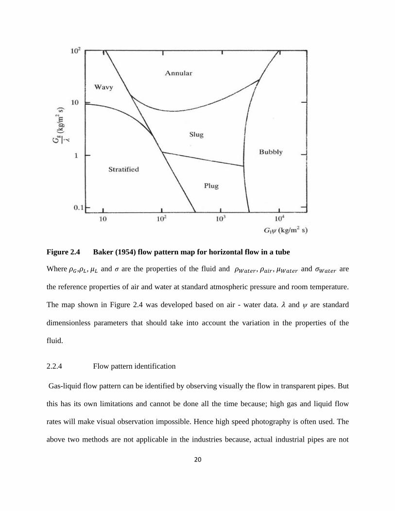
3.3.5 Lengths of the slug unit, the Taylor bubble and the liquid slug
From the relation
where is the length of slug unit, is the time for a particular slug
to pass the probe. But frequency
Therefore
The length of slug unit is therefore calculated from equation (3.8)
Again for an individual slug unit, assuming steady state so that the front and back of the slug
have the same velocity
Dividing equation (3.10) by equation (3.11) results in the following expression
But

42
Finally, substituting equation (3.13) into equation (3.14) and re-arranging results in the following
expressions
The lengths of the liquid slug and Taylor bubble are estimated from equation (3.15) and equation
(3.16) respectively.
3.4 Summary
This chapter has presented both the experimental facility and instrumentation used for
measurements. It also includes the parameters that were needed in the analysis and discussion.
The ensuing chapter deals with the processing of new raw data into required parameters and
analysis of the results.

43
CHAPTER 4
RESULTS AND DISCUSSION
4.1 Analysis of length; liquid slug, Taylor bubble and slug unit
The measured velocities and slug frequencies, the mean length of each Taylor bubble, liquid slug
and slug unit are presented here. The lengths of liquid slug and slug unit can be observed to
increase as the gas superficial velocity increases, for a constant liquid superficial velocity for
both the 0o and 30
o pipe inclination angles. However, at lower constant liquid superficial
velocities of 0.05 and 0.09-m/s the increment is not high in both the length of liquid slug and
slug unit as shown in figures 4.1 and 4.2. It is interesting to notice that as gas superficial velocity
increases to 2.14- m/s at both liquid superficial velocities of 0.28- m/s and 0.38- m/s both the 0o
and 30o
has the same- lengths of liquid slug and slug unit. But on the other hand, the length of the
Taylor bubble did not depict the same trend as gas superficial velocity increases as shown in
figure 4.1.

44
Figure 4.1 a plot of length of liquid slug against gas superficial velocity for various liquid superficial velocities
0
20
40
60
80
100
120
140
160
0 1 2 3 4 5
L
iqu
id s
lug l
ength
[m
]
Gas Superficial Velocity,m/s
Usl=0.05 m/s
0 Degrees
30 degrees
0
0.5
1
1.5
2
2.5
3
3.5
4
4.5
0 1 2 3 4 5
L
iqu
id s
lug l
ength
[m
]
Gas Superficial Velocity,m/s
Usl=0.28 m/s
0 Degrees
30 Degrees
0
20
40
60
80
100
120
0 1 2 3 4 5
L
iqu
id s
lug l
ength
[m]
Gas Superficial Velocity,m/s
Usl=0.09 m/s
0 Degrees
30 Degrees
0
0.5
1
1.5
2
2.5
3
3.5
4
4.5
0 1 2 3 4 5
L
iqu
id s
lug l
ength
[m]
Gas Superficial Velocity,m/s
Usl=0.38 m/s
0 Degrees
30 Degrees

45
Figure 4.2 a plot of length of slug unit against gas superficial velocity for various liquid superficial velocities
0
20
40
60
80
100
120
140
160
0 1 2 3 4 5
Len
gth
of
slu
g u
nit
Gas Superficial Velocity,m/s
Usl=0.05 m/s
0 Degrees
30 Degrees
0
0.5
1
1.5
2
2.5
3
3.5
4
4.5
5
0 1 2 3 4 5
Len
gth
of
slu
g u
nit
Gas Superficial Velocity,m/s
Usl=0.28 m/s 0 Degrees
30 Degrees
0
20
40
60
80
100
120
0 1 2 3 4 5
Len
gth
of
slu
g u
nit
Gas Superficial Velocity,m/s
Usl=0.09 m/s
0 Degrees
30 Degrees
0
1
2
3
4
5
6
0 1 2 3 4 5
Len
gth
of
slu
g u
nit
Gas Superficial Velocity,m/s
Usl=0.38 m/s 0 Degrees
30 Degrees

46
Figure 4.3 a plot of length of Taylor bubble against gas superficial velocity for various liquid superficial velocities
0
5
10
15
20
25
30
0 1 2 3 4 5
Len
gth
of
Taylo
r b
ub
ble
[m
]
Gas Superficial Velocity,m/s
Usl=0.05 m/s
0 degrees
30 degrees
0
0.2
0.4
0.6
0.8
1
1.2
1.4
1.6
1.8
2
0 1 2 3 4 5
Len
gth
of
Taylo
r b
ub
ble
[m
]
Gas Superficial Velocity,m/s
Usl=0.28 m/s
0 Degrees
30 Degrees
0
10
20
30
40
50
60
70
0 1 2 3 4 5
Len
gth
of
Taylo
r b
ub
ble
[m]
Gas Superficial Velocity,m/s
Usl=0.09 m/s 0 Degrees
30 Degrees
0
0.2
0.4
0.6
0.8
1
1.2
1.4
1.6
0 1 2 3 4 5L
ength
of
Taylo
r b
ub
ble
[m]
e
Gas Superficial Velocity,m/s
Usl=0.38 m/s 0 Degrees
30 Degrees

47
It can be concluded therefore that at a given liquid flow rate, a strong relationship exist between
the plot of lengths of liquid slug and slug unit against the gas superficial velocity for 0o
pipe
inclination angle but the relationship is not as strong as in 30o
pipe inclination at lower liquid
flow rate. However, when the gas superficial velocity increases, there is a corresponding
proportional increase in lengths of liquid slug and slug unit at both higher liquid flow rate of
0.38-m/s and this may be attributed to an increase in bubble coalescence as a result of increasing
gas flow rate. The length of the Taylor bubble was observed to reduce with an increase in gas
superficial velocity for the 0o
pipe inclination at all liquid flow rate considered not the same in
the case of 30o
pipe inclination angle. The above observation can be explained by the fact that,
the frequency of the slugging upsurges with increasing gas superficial velocity. Also for a given
flow condition, the slug length keeps fluctuating as a result of continuous interaction between the
phases at the tail of the Taylor bubble. The above conclusions are similar to observation reported
by Hernandez-Perez (2008) and Abdulkadir (2011).
4.2 Time and space average analysis
The ECT used in the experiment provides data that is resolved in time and about a
cross-section with several levels of averaging in time and space. The mean void fraction is
obtained from the liquid hold up and then by averaging the time series data from the ECT. The
time and space averaged information results in a liquid holdup which is widely used in many
engineering estimation of pressure drop, void fraction, interfacial area calculation and heat
transfer. Figure 4.4 shows a plot of mean void fraction against gas superficial velocity for
air/silicone at an angle of inclination of and for various liquid and gas superficial
velocities. The figure shows that, at liquid superficial velocity of 0.05-m/s, the mean void
fraction begins from 0.37 at a gas superficial velocity of 0.047-m/s extending to a maximum

48
value of 0.734 at gas superficial velocity of 4.727-m/s for an inclination of . On the other hand,
for the pipe inclination, the average void fraction begins at 0.074 extending to a maximum
value of 0.818 at gas superficial velocity of 4.727-m/s. It can be concluded therefore that an
increase in pipe inclination from to brings about a corresponding reduction in average
void fraction. However, the observed trend changes as the gas superficial velocity increases from
2.886 m/s thereby causing the inclination to have a lower average void fraction-In addition,
for liquid superficial velocities of 0.09, 0.28 and 0.38-m/s, the initial average void fractions
begins at - 0.08, 0.669 and 0.062, respectively for the inclination whereas it starts at 0.0576,
0.423, and 0.0404, respectively for the pipe inclination. This observed trend is similar to what
is obtainable for the pipe inclination at a liquid superficial velocity of 0.05- m/s where a
decrease in average void fraction at the higher gas superficial velocity is seen. It can be
concluded from the plots that, the trend of mean void fractions is the same for all the inclinations
considered for this work. This may be due to the fact that an increase in the gas superficial
velocity may increase bubble population there by bringing about an increase in average void
fraction. The statement above confirms the conclusions of Hernandez-Perez et al. (2010) that the
average void fraction distribution is strongly affected by pipe inclination, but does not strongly
affect the bubble size distribution.

49
Figure 4.4 Effect of gas superficial velocity and angle of inclination on average void fraction at different liquid superficial velocity
0
0.1
0.2
0.3
0.4
0.5
0.6
0.7
0.8
0.9
0 1 2 3 4 5
Mea
n V
oid
Fra
ctio
n
Gas Superficial Velocity,m/s
Usl=0.05 m/s
0 inclination
30 inclination
0
0.2
0.4
0.6
0.8
1
1.2
0 1 2 3 4 5
Mea
n V
oid
Fra
ctio
n
Gas Superficial Velocity,m/s
Usl=0.28 m/s 0 Inclination
30 Inclination
0
0.1
0.2
0.3
0.4
0.5
0.6
0.7
0.8
0.9
0 1 2 3 4 5
Mea
n V
oid
Fra
ctio
n
Gas Superficial Velocity,m/s
Usl=0.09 m/s 0 Inclination
30 Inclination
0
0.1
0.2
0.3
0.4
0.5
0.6
0.7
0.8
0 1 2 3 4 5M
ean
Void
Fra
ctio
n
Gas Superficial Velocity,m/s
Usl=0.38 m/s 0 Inclination
30 Inclination

50
4.2.1 Mean void fraction from empirical correlations
This section deals with estimation of average void fraction using empirical correlations
which are mostly employed in the industry. Figure 4.5(a) and (b) shows a comparison of
experimental ECT data with empirical models reported in literature. The empirical models
considered are as follows- Guzhov et al.(2000), Greskovich & Cooper (1975), Flanigan (1958)
, Gomez et al (2000), Kokal & Stanislav (1989), Zuber and Findlay (1965), Flanigan (1958) ,
Bonnecaze et al.(1971) and Clark &Flemmer (1985) .
Figure 4.5 (a) Experimental void fraction against empirical models for the inclination
0
0.1
0.2
0.3
0.4
0.5
0.6
0.7
0.8
0.9
1
0 0.2 0.4 0.6 0.8 1
Est
imate
d V
oid
Fra
ctio
n
Experimental Void Fraction
Guzhov et al
Greskovich andCooperFlanigan
Gomez et al
Kokal and Stanislav
Zuber and Findlay
Bonnecaze et al
Clark and Flemme

51
Figure 4. 5 (b) Experimental void fraction against empirical models for the
inclination
The mathematical relation used to estimate Average Root Mean Square (ARMS) is given by
√
∑
ARMS measure the data dispersion around zero deviation, in which; e is the difference between
experimental and estimated data.
[ ]
Table 4.1 Average root mean square (ARMS) of empirical correlation for the 0o and
30o pipe inclination angles
0
0.1
0.2
0.3
0.4
0.5
0.6
0.7
0.8
0.9
1
0 0.2 0.4 0.6 0.8 1
Est
imate
d V
oid
Fra
ctio
n
Experimental Void Fraction
Guzhov et al
Greskovich and
Flanigan
Gomez et al
Kokal and Stanislav
Zuber and Findlay
Bonnecaze et al
Clark and Flemme

52
Correlation 0o 30
o
Guzhov et al. (1967) 4.31 10.58
Greskovich and Cooper (1975) 6.64 13.95
Flanigan(1958) 5.02 6.09
Gomez et al.(2000) 11.17 23.24
Kokal and Stanislav(1989) 6.25 22.44
Zuber and Findlay (1965) 5.04 15.54
Bonnecaze et al. 7.92 23.59
Clark and Flemme 7.67 26.41
Figure 4.6 RMS of empirical correlation
0
5
10
15
20
25
30
RM
S E
rror
[%]
Empirical Correlation
0 Degrees
30 Degrees

53
The correlations used are based on the drift-flux model explained in detail in Chapter two. It is
interesting to know that there is no particular correlation that gave better results in the two
inclination angles considered in this work. It is worth mentioning that a general type correlation
given by Flanigan-(1958) assumes that pipe inclination has no effect on average void fraction.-
However, as can be noticed from Table 4.1 the RMS values are 5.02-% and 6.09-%, respectively
for the inclination angles considered. Most of the correlations that are used in the industry does
not take into consideration pipe inclination. The very few that take into consideration angle of
inclination are Greskovich and Cooper (1975) and Gomez et al. (2000). It is however interesting
to know that for the Greskovich and Cooper (1975) correlation the RMS is lower for
inclination and then increases to 13.95-% for the inclination angle. These deductions can be
attributed to the conditions under which the researcher’s experiments were performed. However,
the general correlation given by Zuber and Findlay (1965), Kokal and Stanislav (1989) gave a
good results for the inclination.-This can be likened to the various conditions under which
each of the researchers conducted their experiment. Though these correlations- did not take into
consideration angle of inclination but rather drift flux.
4.3 Void fraction analysis
Void fraction is an important parameter to characterize two phase flow. It is used to
determine parameters such as two-phase density, two-phase viscosity, and average velocity
among others. It can be seen from figure 4.7 that the void fraction in the liquid slug is directly
proportional to the gas superficial velocity for a constant liquid superficial velocity for both
and pipe inclination angles. However at 2.4-m/s, gas superficial velocity both and
pipe inclination angles have the same average void fraction in the liquid slug. This may be due to
the fact that any increase in the gas flow rate may increase bubble formation, hence causing an
54
increase in the average void fraction. This is a confirmation made by researchers like Nicklin et
al. (1962) and Mao and Dukler (1991). On the other hand, the liquid flow rate has a minimal
influence on the void fraction in the liquid slug. In the case of the void fraction in the Taylor
bubble it can be seen from figure 4.8 that the void fraction in the Taylor bubble increases as the
gas velocity increases for both and pipe inclination angles. It was noted that, the void
fraction in the Taylor bubble fluctuates in both and pipe inclination for all the liquid
superficial velocities considered. It was also observed that, increasing gas flow rate resulted in
more bubbles formation in the liquid slug, which may eventually coalesce with the Taylor bubble
hence increases its void fraction. It is worthy of mention that a decrease in void fraction may
occur when there is a collapse of Taylor bubble signifying a transition to a spherical cap bubble.

55
Figure 4.7 a plot of void fractions in the Taylor bubbles against gas superficial velocity for various liquid superficial
velocities
0
0.2
0.4
0.6
0.8
1
0 1 2 3 4 5
Void
Fra
ctio
n i
n T
aylo
r
Bu
bb
le
Gas Superficial Velocity,m/s
Usl=0.05 m/s 0 Degrees
30 Degrees
0
0.1
0.2
0.3
0.4
0.5
0.6
0.7
0.8
0.9
0 1 2 3 4 5
Void
Fra
ctio
n i
n T
aylo
r
Bu
bb
le
Gas Superficial Velocity,m/s
Usl=0.28 m/s 0 Degrees
30 Degrees
0
0.1
0.2
0.3
0.4
0.5
0.6
0.7
0.8
0.9
1
0 1 2 3 4 5
Void
Fra
ctio
n i
n T
aylo
r
Bu
bb
le
Gas Superficial Velocity,m/s
Usl=0.09 m/s 0 Degrees
30 degrees
0
0.1
0.2
0.3
0.4
0.5
0.6
0.7
0.8
0.9
0 1 2 3 4 5V
oid
Fra
ctio
n i
n T
aylo
r
Bu
bb
le
Gas Superficial Velocity,m/s
Usl=0.38 m/s 0 Degrees
30 Degrees

56
Figure 4.8 a plot of void fractions in the liquid slug against gas superficial velocity for various liquid superficial velocities
0
0.1
0.2
0.3
0.4
0.5
0.6
0.7
0.8
0 1 2 3 4 5Void
Fra
ctio
n i
n L
iqu
id S
lug
Gas Superficial Velocity,m/s
Usl=0.05 m/s
0 Degrees
30 Degrees
0
0.1
0.2
0.3
0.4
0.5
0.6
0.7
0 1 2 3 4 5Void
Fra
ctio
n i
n L
iqu
id S
lug
Gas Superficial Velocity,m/s
Usl=0.28 m/s 0 Degrees
30 Degrees
0
0.1
0.2
0.3
0.4
0.5
0.6
0.7
0 1 2 3 4 5
Void
Fra
ctio
n i
n L
iqu
id S
lug
Gas Superficial Velocity,m/s
Usl=0.09 m/s
0 Degrees
30 Degrees
0
0.1
0.2
0.3
0.4
0.5
0.6
0.7
0 1 2 3 4 5
Void
Fra
ctio
n i
n L
iqu
id S
lug
Gas Superficial Velocity,m/s
Usl=0.38 m/s 0 Degrees
30 Degrees

57
4.4 Pressure drop
Pressure drop is an important parameter in pipeline design. It is an essential variable for the
determination of the pumping energy for a given flow. The diversity of techniques used by
different authors to present two-phase flow pressure drop indicates, that pressure drop in two-
phase flow can depend on a significant number of variables such as gravity. The effect of gravity
on pressure drop is intuitive. Figure 4.9 and 4.10 shows a plot of frictional, accelerational and
gravitational pressure gradients for and pipe inclination angles determined using the
Beggs and Brill (1973) correlation.

58
Figure 4.9 Influence of gas superficial velocity on gravitational and frictional pressure gradient
0
100
200
300
400
500
600
700
800
900
0 1 2 3 4 5
Garv
itati
on
al
pre
ssu
re
dro
p [
Pa/m
]
Gas superficial velocity [m/s]
0 Inclination
30 Inclination
0
100
200
300
400
500
600
700
800
900
0 1 2 3 4 5 6
Garv
itati
on
al
pre
ssu
re
dro
p [
Pa/m
]
Mixture superficial velocity [m/s]
0 Inclination
30 Inclination
0
50
100
150
200
250
300
350
0 1 2 3 4 5
Fri
ctio
nal
pre
ssu
re d
rop
[Pa/m
]
Gas superficial velocity [m/s]
0 Inclination
30 Inclination
0
50
100
150
200
250
300
350
0 1 2 3 4 5 6
Fri
ctio
nal
pre
ssu
re d
rop
[Pa/m
] Mixture superficial velocity [m/s
0 Inclination
30 Inclination
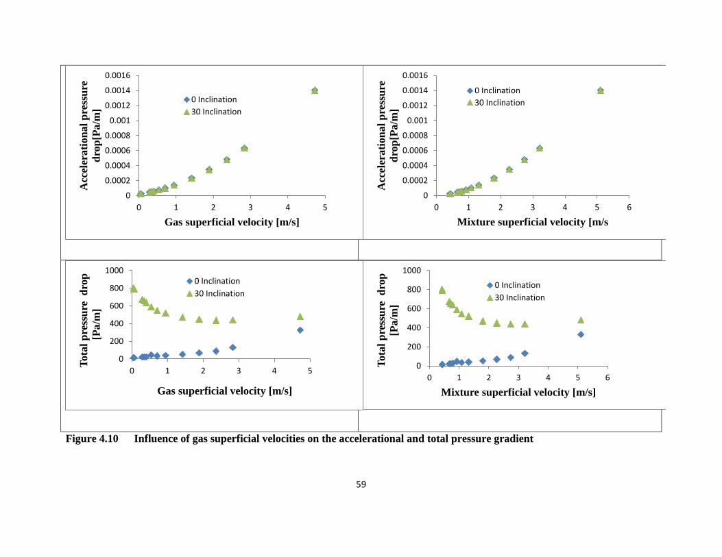
59
Figure 4.10 Influence of gas superficial velocities on the accelerational and total pressure gradient
0
0.0002
0.0004
0.0006
0.0008
0.001
0.0012
0.0014
0.0016
0 1 2 3 4 5
Acc
eler
ati
on
al
pre
ssu
re
dro
p[P
a/m
]
Gas superficial velocity [m/s]
0 Inclination
30 Inclination
0
0.0002
0.0004
0.0006
0.0008
0.001
0.0012
0.0014
0.0016
0 1 2 3 4 5 6
Acc
eler
ati
on
al
pre
ssu
re
dro
p[P
a/m
]
Mixture superficial velocity [m/s
0 Inclination
30 Inclination
0
200
400
600
800
1000
0 1 2 3 4 5 T
ota
l p
ress
ure
d
rop
[Pa/m
]
Gas superficial velocity [m/s]
0 Inclination
30 Inclination
0
200
400
600
800
1000
0 1 2 3 4 5 6T
ota
l p
ress
ure
d
rop
[Pa
/m]
Mixture superficial velocity [m/s]
0 Inclination
30 Inclination

60
Figures 4.9 and 4.10 clearly indicates that for the inclination angle, the main contributor to the
total pressure gradient is the frictional shear stress and acceleration component, which is
dependent on the mixture density, which in turn is a function of the in-situ volume fraction or
liquid holdup. However, there is an increase in total pressure gradient when the inclination angle
increases from to as depicted from the above Figure 4.9 and 4.10.
It is interesting to note that for a given liquid superficial velocity, there is no great effect in both
the frictional and acceleration pressure gradient as gas superficial velocity increases in the two
inclination angles considered. However, in the case of the gravitational component there exist
increase in pressure gradient as both gas and mixture superficial velocities increases. This
contributes to the overall total pressure gradient predicted in the angles considered in this
experiment. Mattar and Gregory (1974), Spedding and Chen (1981), Barnea et al (1985),
Roumazeilles et al. (1994) concluded in their work that larger bubbles are formed due to
coalescence, which causes a decrease in the liquid velocity due to higher level of liquid holdup,
hence increasing the frictional pressure gradient.
4.5 Structure velocity
A cross-correlation was performed between the time varying void fraction data measured by the
twin ECT-planes positioned at 4.400 m and 4.489 m above the mixing chamber at the bottom of
the riser. The evaluation of the time delay for individual slug to travel from ECT-plane-1 to
ECT-plane-2 facilitated the computation of the translational velocity. A plot of structure velocity
is plotted against mixture superficial velocity (where ) as shown in Figure 4.12.
A comparison between the structure velocities obtained
from experiment and two major correlations is also presented here . The two correlations
Bediksen (1984) and Nicklin et al. (1962) are and

61
, respectively- Where, is the mixture velocity, g is the acceleration due to gravity
and D is the pipe diameter.
Figure 4. 11 Structure velocity for 0o
and 30o inclination angles obtained from
experiments using ECT and empirical correlations of Bendiksen (1984) and Nicklin et al.
(1962) correlation
Figure 4.11 shows that both the Nicklin et al. (1962) and Bendiksen (1984) correlations predict
well for both the 0o
and 30o
inclination angles, even though the correlation of Nicklin et al.
(1962) as reported in the literature to be applicable to vertical pipes. Interestingly, in this study
this correlation has been able to predict structure velocity close to the general Bendiksen
correlation for predicting structure velocity-for all pipe orientations.
0
1
2
3
4
5
6
7
0 2 4 6
Str
uct
ure
Vel
oci
ty [
m/s
]
Mixture Velocity [m/s]
0 Degrees
30 Degrees
Bendiksen (1984)
Nicklin et al.(1962)

62
4.6 Flow pattern map
Flow pattern map determines the transition boundaries between the different flow pattern regions
as a function of the gas and liquid superficial velocities. In predicting the flow pattern map using
Shoham (2006) computer codes, the fluid properties consisting of density, viscosity and surface
tension were specified in the input data interface. The pipe geometry was also specified by
diameter, angle and absolute roughness with the interface also specified as smooth. The
calculated boundaries are then plotted in the form of a flow pattern map using and as
coordinate system. The operating point will be overlaid on the general flow pattern map and the
existing flow pattern can be observed on the map. Figure 4.12 (a) and (b) show the flow pattern
map generated for and pipe inclination angle. The model adopted here was based on Taitel
et al. (1980) for bubbly/slug transition. Moreover, slug flow was the most dominant flow pattern
as observed in both inclination angles, characterized with occurrence of Taylor bubbles. The
other models that could be adopted for other flow regimes are Jayanti and Hewitt (1992) or
Watson and Hewitt (1999) model based on slug and churn flow transition. The flow rates at
which the experiment was carried out by Abdulkadir (2011a) for liquid and gas superficial
velocity were in the range of 0.38m/sUm/s05.0 SL and 4.727m/sUm/s047.0 SG
respectively

63
(a) (b)
Figure 4.12 (a) and (b)Shoham (2006) flow pattern map for and air/silicone
mixture
From the flow pattern map shown in figures 4.12(a) and (b) at inclination most of the
data points were between stratified smooth flow and slug flow regions at liquid velocity between
0.05 to 0.38- m/s. The data points that fell in the slug region can be attributed to the increase in
liquid velocity from 0.28 to 0.38 -m/s. However, for the pipe inclined at 30 o
to the horizontal all
the data points fell in the region of slug flow as seen in figure 4.12 (b) at the same conditions.
This confirms at very small inclination angles, the force of gravity acting in the flow direction
can be of the order of the wall shear stress. This interesting observation is in agreement with the
conclusions made by Barnea et al (1985) in their work. This also confirms the conclusions made
by Mattar and Gregory (1974) that for uphill pipe sections, slug flow was the predominant flow
pattern.
0.001
0.01
0.1
1
10
0.01 0.1 1 10 100
Gas Superficial Velocity,Usg, m/s
Liq
uid
Su
per
ficia
l Vel
oci
ty,U
SL
, m/s
Stratified
(A-L)
Annular
(J)
Wavy
(C-K)
Dispersed-
Bubble
(F-G)Bubble
(E)
Operating
Points
0.001
0.01
0.1
1
10
0.01 0.1 1 10 100
Gas Superficial Velocity,Usg, m/s
Liq
uid
Su
per
ficia
l Vel
oci
ty,U
SL
, m/s
Stratified
(A-L)
Annular
(J)
Wavy
(C-K)
Dispersed-
Bubble
(F-G)Bubble
(E)
Operating
Points

64
4.7 Probability density function (PDF)
PDF reveals information about the frequency of occurrence of each void fraction through
amplitude and time variation. Figure 4.13 shows a series of curves at different gas superficial
velocities with a constant liquid superficial velocity of 0.38 m/s. Discrete random variables can
be plotted in a histogram which shows the frequency (on the ordinate) as a function of
some measured parameter (on the abscissa for a given class width). The frequency distribution
is then a collection of classes which are of equal size and cover the entire range of data
without over lapping. The PDF with a high and a low peak indicate slug flow. However, they
are not clear as those of Costigan and Whalley (1997) and Omebere-Iyari and Azzopardi (2006)
who worked with pipes of smaller internal diameter than the present work. Khatib and
Richardson (1984) and Costigan and Whalley (1997) proposed that twin peaked probability
density function (PDFs) of recorded void fractions represented slug flow. The low void fraction
peak corresponds to liquid slug while the high void fraction peak is for the corresponding Taylor
bubble.

65
RUN 0o Inclination 30
o Inclination
66
68
0
0.05
0.1
0.15
0.2
0.25
0.3
0 0.2 0.4 0.6 0.8 1Pro
bab
ilit
y D
ensi
ty
Fu
nct
ion
(P
DF
)
Void Fraction
Usg=0.047 m/s
Usl=0.38 m/s
0
0.1
0.2
0.3
0.4
0.5
0.6
0 0.2 0.4 0.6 0.8 1
Pro
bab
ilit
y D
ensi
ty F
un
ctio
n
(PD
F)
Void Fraction
Usg=0.047 m/s
Usl=0.38 m/s
0
0.05
0.1
0.15
0 0.2 0.4 0.6 0.8 1Pro
bab
ilit
y D
ensi
ty
Fu
nct
ion
(P
DF
)
Void Fraction
Usg=0.288 m/s
Usl=0.38 m/s
0
0.02
0.04
0.06
0.08
0.1
0 0.2 0.4 0.6 0.8 1
Pro
bab
ilit
y D
ensi
ty F
un
ctio
n
(PD
F)
Void Fraction
Usg=0.288 m/s
Usl=0.38 m/s

66
73
78
Figure 4.13 PDF for 0o and 30
o pipe inclination
0
0.01
0.02
0.03
0.04
0.05
0.06
0 0.2 0.4 0.6 0.8 1
Pro
bab
ilit
y D
ensi
ty F
un
ctio
n
(PD
F)
Void Fraction
Usg=0.945 m/s
Usl=0.38 m/s
0
0.005
0.01
0.015
0.02
0.025
0.03
0 0.2 0.4 0.6 0.8 1
Pro
bab
ilit
y D
ensi
ty F
un
ctio
n
(PD
F)
Void Fraction
Usg=0.945 m/s
Usl=0.38 m/s
0
0.02
0.04
0.06
0.08
0.1
0 0.2 0.4 0.6 0.8 1
Pro
bab
ilit
y D
ensi
ty F
un
ctio
n
(PD
F)
Void Fraction
Usg=4.727m/s
Usl=0.38 m/s
0
0.01
0.02
0.03
0.04
0.05
0.06
0.07
0 0.2 0.4 0.6 0.8 1P
rob
ab
ilit
y D
ensi
ty F
un
ctio
n
(PD
F)
Void Fraction
Usg=4.727 m/s
Usl=0.38 m/s

67
4.8 Frequency
Gregory and Scott (1969) developed a much used correlation for slug frequency prediction based
on the data by Hubbard (1965). The methodology of power spectral density (PSD) was used to
determine the dominant frequency. Details of PSD can be found in Hubbard and Duckler (1966).
The outputs from the measuring instruments were analyzed and their plots were compared
for various inclination considered in this work as shown in figure 4.14 for various liquid
superficial velocities using ECT.

68
Figure 4.14 Effect of gas superficial velocity and angle of inclination on frequency for various liquid superficial velocity
0
0.2
0.4
0.6
0.8
1
1.2
1.4
1.6
1.8
2
0 1 2 3 4 5 6
Fre
qu
ency
Gas Superficial Velocity,m/s
Usl=0.05 m/s 0 Inclination
30 Inclination
0
0.5
1
1.5
2
2.5
3
0 1 2 3 4 5 6
Fre
qu
ency
Gas Superficial Velocity,m/s
Usl=0.28 m/s 0 Inclination
30 Inclination
0
0.5
1
1.5
2
2.5
0 1 2 3 4 5 6
Fre
qu
ency
Gas Superficial Velocity,m/s
Usl=0.09 m/s 0 Inclination
30 inclination
0
0.5
1
1.5
2
2.5
3
3.5
0 1 2 3 4 5 6
Fre
qu
ency
Gas Superficial Velocity,m/s
Usl=0.38 m/s 0 Inclination
30 Inclination
69
Figure 4.14 shows that at constant liquid superficial velocity of 0.05-m/s and inclination there
is a constant frequency of 0.0166-Hz for the range of considered. However, in the case of
inclination angle there is a decrease in frequency from 1.9 - 0.86- Hz at the same constant liquid
superficial velocity. Increasing the liquid superficial velocity from 0.05-0.38 m/s brings about an
increase in frequency for the and inclination angles.

70
CHAPTER 5
CONCLUSIONS AND RECOMMENDATIONS
In this work an extensive study of effect of pipe inclination has been presented. Liquid
holdup, pressure drop, structure velocity and frequency for different inclination angles and flow
rates were estimated using experimental data. These data were then analyzed. The analysis
was carried out by varying liquid and gas velocities and inclination. This has given a good
insight into the phenomena that occur in inclined pipes. The summarized points below in this
chapter give the final conclusions drawn from this study. Further work is also proposed, in order
to improve and expand the knowledge of multiphase flow in inclined pipes.
5.1 Conclusions
Pipe inclination effect has been successfully investigated using ECT instrument. From the
analysis made in chapter four it can be concluded- that pipe- inclination has some effects on
the gas-liquid flows. The lengths of the Taylor bubbles, and the slug units were found to
increase with increasing gas superficial velocity. Though, the length of the liquid slug was
found to be varying due to a coalescence of the dispersed bubbles from the wake of a Taylor
bubble.
The slug frequency was found to generally decrease with increasing gas superficial velocity
at lower liquid superficial velocity. However, at higher liquid superficial velocities, the slug
frequency increases with increasing gas superficial velocity.
Beggs and Brill (1973) correlation for pressure gradient prediction was used to calculate the
pressure gradient in this study. The correlation predicts that as the pipe inclination increases

71
from 0o
to 30o there is a general increase in gravitational, frictional and acceleration pressure
drop, hence an increase in the overall total pressure drop.
In this work none of the void fraction correlation predicted perfectly for both the 0o
and 30o
pipe inclination. However,-Guzhov et al. (1967) and Flanigan (1958) are the best
performing correlation based on the drift flux model for both inclination.
A linear relationship was obtained between structure velocity and mixture superficial
velocity. A comparison of this data with the empirical relationships proposed the Nicklin et
al. (1962) and Bendiksen (1984) correlations predict well for both the 0o
and 30o
inclination
angles. Even though the correlation of Nicklin et al. (1962) as reported in the literature to be
applicable to vertical pipes.
5.2 Recommendations
A similar comparative analysis should be carried out on the effect of pipe inclination on-
void fraction distributions for inclinations higher than 30o.
Investigating the effect of fluid properties (density, viscosity, and surface tension) would be
of particular interest in the oil and gas industry applications where liquids and gases have
different properties.
Finally, computational fluid dynamics should be employed to validate the void fraction
distribution in pipe inclination.

72
NOMENCLATURE
Symbol Description Units
A Cross-sectional Area
Distribution parameter Dimensionless
D Diameter of pipe m
Liquid-holdup Dimensionless
Froude number,
Dimensionless
f Frequency
g Acceleration of gravity
G Mass flux
L Length m
m Mass
Density
Mixture Reynolds number Dimensionless
S Slip ratio Dimensionless
Viscosity
Velocity of gas
Drift velocity,
Velocity of liquid
Mixture velocity,
Superficial gas velocity
Superficial Liquid velocity

73
X quality, mass of Vapour /total mass Dimensionless
T Temperature
P Pressure
Greek Letters
Void fraction, average
No slip (homogeneous) void fraction
Volumetric quality, H
Input liquid content,
Viscosity
Density
Pipe inclination angle
Subscripts
G Gas Phase
L Liquid Phase
M Mixture
S Superficial

74
APPENDICES
APPENDIX A DATA TEST MATRIX FOR 67mm 0o PIPE INCLINATION
RUN Usl[m/s] Usg[m/s] Um[m/s] HL ε Freq[Hz] δ[mm]
Structural
velocity Bendiksen Nicklin
1 0.05 0.047 0.097 0.6274 0.3726 0.01667 13.0513 -0.084 0.55419 0.40015
2 0.05 0.061 0.111 0.6324 0.3676 0.01667 13.1889 0.6 0.57099 0.41695
3 0.05 0.288 0.338 0.5387 0.4613 0.01667 10.7471 0.73 0.84339 0.68935
4 0.05 0.344 0.394 0.5155 0.4845 0.01667 10.182 0.8 0.91059 0.75655
5 0.05 0.404 0.454 0.4834 0.5166 0.01667 9.42191 0.88 0.98259 0.82855
6 0.05 0.544 0.594 0.4111 0.5889 0.01667 7.79216 0.88 1.15059 0.99655
7 0.05 0.709 0.759 0.3731 0.6269 0.01667 6.9757 1.2 1.34859 1.19455
8 0.05 0.945 0.995 0.3312 0.6688 0.01667 6.10364 1.53 1.63179 1.47775
9 0.05 1.418 1.468 0.2384 0.7616 0.01667 4.26465 1.87 2.19939 2.04535
10 0.05 1.891 1.941 0.223 0.777 0.01667 3.97055 2.4 2.76699 2.61295
11 0.05 2.363 2.413 0.1698 0.8302 0.01667 2.97637 2.4 3.33339 3.17935
12 0.05 2.836 2.886 0.2196 0.7804 0.01667 3.90602 2.4 3.90099 3.74695
13 0.05 4.727 4.777 0.2652 0.7348 0.01667 4.78364 0.48 6.17019 6.01615

75
27 0.09 0.047 0.137 0.9144 0.0856 0.01667 23.6987 0.73 0.60219 0.44815
28 0.09 0.061 0.151 0.8996 0.1004 0.01667 22.8852 0.76 0.61899 0.46495
29 0.09 0.288 0.378 0.7049 0.2951 0.01667 15.3018 1.05 0.89139 0.73735
30 0.09 0.344 0.434 0.6594 0.3406 0.01667 13.9491 1.12 0.95859 0.80455
31 0.09 0.404 0.494 0.6254 0.3746 0.01667 12.9965 1.2 1.03059 0.87655
32 0.09 0.544 0.634 0.531 0.469 0.01667 10.558 1.4 1.19859 1.04455
33 0.09 0.709 0.799 0.4774 0.5226 0.01667 9.28249 1.53 1.39659 1.24255
34 0.09 0.945 1.035 0.4277 0.5723 0.01667 8.15708 1.87 1.67979 1.52575
35 0.09 1.418 1.508 0.2963 0.7037 0.55 5.39791 2.1 2.24739 2.09335
36 0.09 1.891 1.981 0.2536 0.7464 0.6 4.55786 2.4 2.81499 2.66095
37 0.09 2.363 2.453 0.2393 0.7607 0.56667 4.28193 2.4 3.38139 3.22735
38 0.09 2.836 2.926 0.2199 0.7801 0.58333 3.9117 2.8 3.94899 3.79495
39 0.09 4.727 4.817 0.3293 0.6707 0.01667 6.06475 1.87 6.21819 6.06415
53 0.28 0.047 0.327 0.9302 0.0698 0.5 24.6494 0.88 0.83019 0.67615
54 0.28 0.061 0.341 0.9171 0.0829 0.56667 23.8546 0.93 0.84699 0.69295
55 0.28 0.288 0.568 0.7316 0.2684 0.63333 16.1445 1.2 1.11939 0.96535
56 0.28 0.344 0.624 0.6947 0.3053 0.63333 14.9899 1.29 1.18659 1.03255

76
57 0.28 0.404 0.684 0.6738 0.3262 0.63333 14.3668 1.29 1.25859 1.10455
58 0.28 0.544 0.824 0.5893 0.4107 0.7 12.0312 1.53 1.42659 1.27255
59 0.28 0.709 0.989 0.5341 0.4659 0.75 10.6339 1.68 1.62459 1.47055
60 0.28 0.945 1.225 0.4581 0.5419 0.83333 8.83936 1.87 1.90779 1.75375
61 0.28 1.418 1.698 0.3525 0.6475 0.85 6.54343 2.4 2.47539 2.32135
62 0.28 1.891 2.171 0.3029 0.6971 0.85 5.53001 2.8 3.04299 2.88895
63 0.28 2.363 2.643 0.2735 0.7265 1.03333 4.94629 2.8 3.60939 3.45535
64 0.28 2.836 3.116 0.2805 0.7195 0.8 5.08418 3.36 4.17699 4.02295
65 0.28 4.727 5.007 0.3725 0.6275 0.65 6.96301 2.4 6.44619 6.29215
66 0.38 0.047 0.427 0.9374 0.0626 0.68333 25.1183 0.99 0.95019 0.79615
67 0.38 0.061 0.441 0.9204 0.0796 0.7 24.0485 1.05 0.96699 0.81295
68 0.38 0.288 0.668 0.7505 0.2495 0.85 16.7668 1.4 1.23939 1.08535
69 0.38 0.344 0.724 0.7249 0.2751 0.86667 15.9293 1.4 1.30659 1.15255
70 0.38 0.404 0.784 0.6976 0.3024 0.81667 15.078 1.53 1.37859 1.22455
71 0.38 0.544 0.924 0.993 0.007 0.9 30.6972 1.68 1.54659 1.39255
72 0.38 0.709 1.089 0.5652 0.4348 0.8 11.4103 1.68 1.74459 1.59055
73 0.38 0.945 1.325 0.4696 0.5304 0.81667 9.10243 2.1 2.02779 1.87375
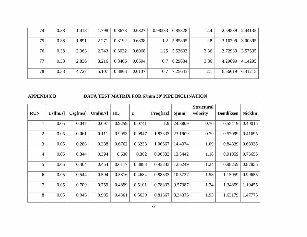
77
74 0.38 1.418 1.798 0.3673 0.6327 0.98333 6.85328 2.4 2.59539 2.44135
75 0.38 1.891 2.271 0.3192 0.6808 1.2 5.85895 2.8 3.16299 3.00895
76 0.38 2.363 2.743 0.3032 0.6968 1.25 5.53603 3.36 3.72939 3.57535
77 0.38 2.836 3.216 0.3406 0.6594 0.7 6.29684 3.36 4.29699 4.14295
78 0.38 4.727 5.107 0.3863 0.6137 0.7 7.25643 2.1 6.56619 6.41215
APPENDIX B DATA TEST MATRIX FOR 67mm 30o
PIPE INCLINATION
RUN Usl[m/s] Usg[m/s] Um[m/s] HL ε Freq[Hz] δ[mm]
Structural
velocity Bendiksen Nicklin
1 0.05 0.047 0.097 0.9259 0.0741 1.9 24.3809 0.76 0.55419 0.40015
2 0.05 0.061 0.111 0.9053 0.0947 1.83333 23.1909 0.79 0.57099 0.41695
3 0.05 0.288 0.338 0.6762 0.3238 1.06667 14.4374 1.09 0.84339 0.68935
4 0.05 0.344 0.394 0.638 0.362 0.98333 13.3442 1.16 0.91059 0.75655
5 0.05 0.404 0.454 0.6117 0.3883 0.93333 12.6249 1.24 0.98259 0.82855
6 0.05 0.544 0.594 0.5316 0.4684 0.88333 10.5727 1.58 1.15059 0.99655
7 0.05 0.709 0.759 0.4899 0.5101 0.78333 9.57387 1.74 1.34859 1.19455
8 0.05 0.945 0.995 0.4361 0.5639 0.81667 8.34375 1.93 1.63179 1.47775
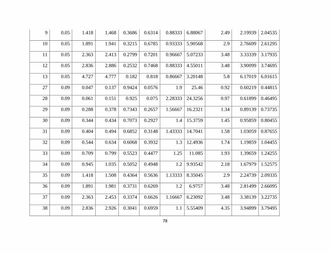
78
9 0.05 1.418 1.468 0.3686 0.6314 0.88333 6.88067 2.49 2.19939 2.04535
10 0.05 1.891 1.941 0.3215 0.6785 0.93333 5.90568 2.9 2.76699 2.61295
11 0.05 2.363 2.413 0.2799 0.7201 0.96667 5.07233 3.48 3.33339 3.17935
12 0.05 2.836 2.886 0.2532 0.7468 0.88333 4.55011 3.48 3.90099 3.74695
13 0.05 4.727 4.777 0.182 0.818 0.86667 3.20148 5.8 6.17019 6.01615
27 0.09 0.047 0.137 0.9424 0.0576 1.9 25.46 0.92 0.60219 0.44815
28 0.09 0.061 0.151 0.925 0.075 2.28333 24.3256 0.97 0.61899 0.46495
29 0.09 0.288 0.378 0.7343 0.2657 1.56667 16.2321 1.34 0.89139 0.73735
30 0.09 0.344 0.434 0.7073 0.2927 1.4 15.3759 1.45 0.95859 0.80455
31 0.09 0.404 0.494 0.6852 0.3148 1.43333 14.7041 1.58 1.03059 0.87655
32 0.09 0.544 0.634 0.6068 0.3932 1.3 12.4936 1.74 1.19859 1.04455
33 0.09 0.709 0.799 0.5523 0.4477 1.25 11.085 1.93 1.39659 1.24255
34 0.09 0.945 1.035 0.5052 0.4948 1.2 9.93542 2.18 1.67979 1.52575
35 0.09 1.418 1.508 0.4364 0.5636 1.13333 8.35045 2.9 2.24739 2.09335
36 0.09 1.891 1.981 0.3731 0.6269 1.2 6.9757 3.48 2.81499 2.66095
37 0.09 2.363 2.453 0.3374 0.6626 1.16667 6.23092 3.48 3.38139 3.22735
38 0.09 2.836 2.926 0.3041 0.6959 1.1 5.55409 4.35 3.94899 3.79495
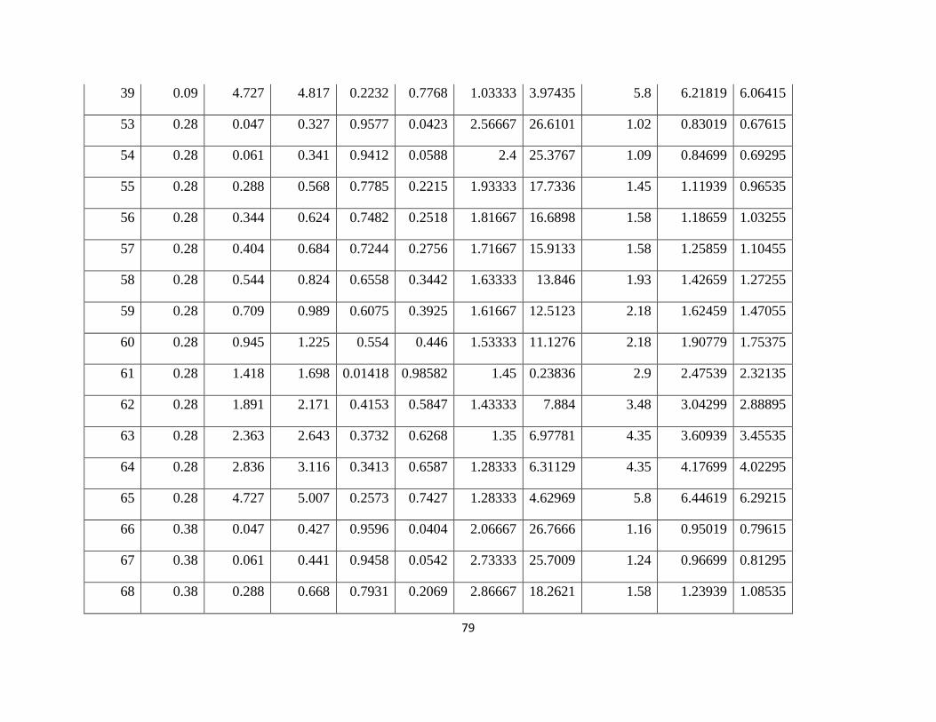
79
39 0.09 4.727 4.817 0.2232 0.7768 1.03333 3.97435 5.8 6.21819 6.06415
53 0.28 0.047 0.327 0.9577 0.0423 2.56667 26.6101 1.02 0.83019 0.67615
54 0.28 0.061 0.341 0.9412 0.0588 2.4 25.3767 1.09 0.84699 0.69295
55 0.28 0.288 0.568 0.7785 0.2215 1.93333 17.7336 1.45 1.11939 0.96535
56 0.28 0.344 0.624 0.7482 0.2518 1.81667 16.6898 1.58 1.18659 1.03255
57 0.28 0.404 0.684 0.7244 0.2756 1.71667 15.9133 1.58 1.25859 1.10455
58 0.28 0.544 0.824 0.6558 0.3442 1.63333 13.846 1.93 1.42659 1.27255
59 0.28 0.709 0.989 0.6075 0.3925 1.61667 12.5123 2.18 1.62459 1.47055
60 0.28 0.945 1.225 0.554 0.446 1.53333 11.1276 2.18 1.90779 1.75375
61 0.28 1.418 1.698 0.01418 0.98582 1.45 0.23836 2.9 2.47539 2.32135
62 0.28 1.891 2.171 0.4153 0.5847 1.43333 7.884 3.48 3.04299 2.88895
63 0.28 2.363 2.643 0.3732 0.6268 1.35 6.97781 4.35 3.60939 3.45535
64 0.28 2.836 3.116 0.3413 0.6587 1.28333 6.31129 4.35 4.17699 4.02295
65 0.28 4.727 5.007 0.2573 0.7427 1.28333 4.62969 5.8 6.44619 6.29215
66 0.38 0.047 0.427 0.9596 0.0404 2.06667 26.7666 1.16 0.95019 0.79615
67 0.38 0.061 0.441 0.9458 0.0542 2.73333 25.7009 1.24 0.96699 0.81295
68 0.38 0.288 0.668 0.7931 0.2069 2.86667 18.2621 1.58 1.23939 1.08535

80
69 0.38 0.344 0.724 0.7658 0.2342 2.23333 17.2879 1.74 1.30659 1.15255
70 0.38 0.404 0.784 0.7429 0.2571 2.15 16.5138 1.74 1.37859 1.22455
71 0.38 0.544 0.924 0.6754 0.3246 1.96667 14.4138 1.93 1.54659 1.39255
72 0.38 0.709 1.089 0.6193 0.3807 1.75 12.8302 2.18 1.74459 1.59055
73 0.38 0.945 1.325 0.572 0.428 1.66667 11.5837 2.49 2.02779 1.87375
74 0.38 1.418 1.798 0.4875 0.5125 1.55 9.51765 2.9 2.59539 2.44135
75 0.38 1.891 2.271 0.4343 0.5657 1.55 8.30363 3.48 3.16299 3.00895
76 0.38 2.363 2.743 0.3923 0.6077 1.58333 7.38504 3.48 3.72939 3.57535
77 0.38 2.836 3.216 0.3632 0.6368 1.35 6.76708 4.35 4.29699 4.14295
78 0.38 4.727 5.107 0.2856 0.7144 1.56667 5.18507 4.21 6.56619 6.41215

81
APPENDIX C BEGGS AND BRILL (1973) CORRELATION FOR
PRESSURE GRADIENT
CORRELATION PREDICTION FOR 67mm 0o PIPE INCLINATION
RUN Usl[m/s] Usg[m/s] Um[m/s] HL (dP/dz)G (dP/dz)F (dP/dz)Acc (dP/dz)T
1 0.05 0.047 0.097 0.6274 0 0.84682 2.24224E-06 0.84682
2 0.05 0.061 0.111 0.6324 0 1.03836 2.72772E-06 1.03837
3 0.05 0.288 0.338 0.5387 0 4.86341 1.49925E-05 4.86343
4 0.05 0.344 0.394 0.5155 0 5.94191 1.91394E-05 5.94193
5 0.05 0.404 0.454 0.4834 0 6.99651 2.40286E-05 6.99653
6 0.05 0.544 0.594 0.4111 0 9.20246 3.71446E-05 9.20249
7 0.05 0.709 0.759 0.3731 0 12.4821 5.54953E-05 12.4822
8 0.05 0.945 0.995 0.3312 0 17.348 8.68467E-05 17.3481
9 0.05 1.418 1.468 0.2384 0 23.9823 0.000166528 23.9825
10 0.05 1.891 1.941 0.223 0 35.977 0.000266963 35.9773
11 0.05 2.363 2.413 0.1698 0 39.7768 0.000386899 39.7772
12 0.05 2.836 2.886 0.2196 0 69.6798 0.000525007 69.6804
13 0.05 4.727 4.777 0.2652 0 200.302 0.001251016 200.303
27 0.09 0.047 0.137 0.9144 0 2.04684 3.72115E-06 2.04684
28 0.09 0.061 0.151 0.8996 0 2.32985 4.30525E-06 2.32985
29 0.09 0.288 0.378 0.7049 0 7.59586 1.79056E-05 7.59587
30 0.09 0.344 0.434 0.6594 0 8.86632 2.23396E-05 8.86634
31 0.09 0.404 0.494 0.6254 0 10.3619 2.75242E-05 10.362
32 0.09 0.544 0.634 0.531 0 13.2043 4.12939E-05 13.2044

82
33 0.09 0.709 0.799 0.4774 0 17.3598 6.03674E-05 17.3599
34 0.09 0.945 1.035 0.4277 0 23.8864 9.26845E-05 23.8865
35 0.09 1.418 1.508 0.2963 0 31.1354 0.000174143 31.1355
36 0.09 1.891 1.981 0.2536 0 42.3092 0.000276271 42.3095
37 0.09 2.363 2.453 0.2393 0 57.4609 0.000397503 57.4613
38 0.09 2.836 2.926 0.2199 0 71.4398 0.000537538 71.4403
39 0.09 4.727 4.817 0.3293 0 251.988 0.001268735 251.989
53 0.28 0.047 0.327 0.9302 0 7.95519 1.42172E-05 7.9552
54 0.28 0.061 0.341 0.9171 0 8.38235 1.51943E-05 8.38237
55 0.28 0.288 0.568 0.7316 0 15.192 3.45071E-05 15.192
56 0.28 0.344 0.624 0.6947 0 16.8166 4.02222E-05 16.8166
57 0.28 0.404 0.684 0.6738 0 18.9549 4.67403E-05 18.955
58 0.28 0.544 0.824 0.5893 0 22.5273 6.34961E-05 22.5274
59 0.28 0.709 0.989 0.5341 0 27.6312 8.59106E-05 27.6312
60 0.28 0.945 1.225 0.4581 0 33.8803 0.000122765 33.8804
61 0.28 1.418 1.698 0.3525 0 45.2 0.000212657 45.2002
62 0.28 1.891 2.171 0.3029 0 58.9679 0.000322659 58.9683
63 0.28 2.363 2.643 0.2735 0 74.5232 0.00045139 74.5236
64 0.28 2.836 3.116 0.2805 0 101.321 0.000598463 101.321
65 0.28 4.727 5.007 0.3725 0 304.63 0.001356556 304.631
66 0.38 0.047 0.427 0.9374 0 12.2675 2.17559E-05 12.2675
67 0.38 0.061 0.441 0.9204 0 12.6863 2.29135E-05 12.6863
68 0.38 0.288 0.668 0.7505 0 20.3034 4.4958E-05 20.3034
69 0.38 0.344 0.724 0.7249 0 22.3802 5.13034E-05 22.3802

83
70 0.38 0.404 0.784 0.6976 0 24.5534 5.84836E-05 24.5534
71 0.38 0.544 0.924 0.993 0 45.8108 7.67009E-05 45.8109
72 0.38 0.709 1.089 0.5652 0 34.3152 0.000100836 34.3153
73 0.38 0.945 1.325 0.4696 0 39.6052 0.000140005 39.6053
74 0.38 1.418 1.798 0.3673 0 51.8711 0.000234247 51.8713
75 0.38 1.891 2.271 0.3192 0 67.0696 0.000348329 67.07
76 0.38 2.363 2.743 0.3032 0 87.9735 0.000480897 87.974
77 0.38 2.836 3.216 0.3406 0 129.731 0.000631602 129.732
78 0.38 4.727 5.107 0.3863 0 326.89 0.001403864 326.892
APPENDIX D BEGGS AND BRILL (1973) CORRELATION FOR
PRESSURE GRADIENT
CORRELATION PREDICTION FOR 67mm 30o PIPE INCLINATION
RUN Usl[m/s] Usg[m/s] Um[m/s] HL (dP/dz)G (dP/dz)F (dP/dz)Acc (dP/dz)T
1 0.05 0.047 0.097 0.9259 762.323 1.24811 2.24093E-06 763.571
2 0.05 0.061 0.111 0.9053 745.387 1.48471 2.7263E-06 746.872
3 0.05 0.288 0.338 0.6762 557.039 6.09969 1.49877E-05 563.139
4 0.05 0.344 0.394 0.638 525.634 7.34794 1.91336E-05 532.982
5 0.05 0.404 0.454 0.6117 504.012 8.84519 2.40203E-05 512.858
6 0.05 0.544 0.594 0.5316 438.16 11.886 3.71292E-05 450.047
7 0.05 0.709 0.759 0.4899 403.878 16.3679 5.54697E-05 420.246
8 0.05 0.945 0.995 0.4361 359.648 22.8087 8.68034E-05 382.457

84
9 0.05 1.418 1.468 0.3686 304.155 36.9703 0.000166369 341.125
10 0.05 1.891 1.941 0.3215 265.433 51.728 0.000266738 317.161
11 0.05 2.363 2.413 0.2799 231.232 65.2735 0.000386369 296.506
12 0.05 2.836 2.886 0.2532 209.282 80.2475 0.000524824 289.53
13 0.05 4.727 4.777 0.182 150.747 137.911 0.001252172 288.659
27 0.09 0.047 0.137 0.9424 775.888 2.10935 3.72103E-06 777.998
28 0.09 0.061 0.151 0.925 761.583 2.39546 4.30511E-06 763.979
29 0.09 0.288 0.378 0.7343 604.805 7.91168 1.79047E-05 612.716
30 0.09 0.344 0.434 0.7073 582.607 9.50827 2.23377E-05 592.116
31 0.09 0.404 0.494 0.6852 564.438 11.3493 2.75212E-05 575.788
32 0.09 0.544 0.634 0.6068 499.984 15.0818 4.12866E-05 515.066
33 0.09 0.709 0.799 0.5523 455.178 20.0716 6.03551E-05 475.25
34 0.09 0.945 1.035 0.5052 416.456 28.194 9.26617E-05 444.651
35 0.09 1.418 1.508 0.4364 359.894 45.7579 0.000174022 405.653
36 0.09 1.891 1.981 0.3731 307.854 62.0913 0.000276057 369.946
37 0.09 2.363 2.453 0.3374 278.504 80.8251 0.000397217 359.33
38 0.09 2.836 2.926 0.3041 251.128 98.5541 0.000537147 349.682
39 0.09 4.727 4.817 0.2232 184.618 171.265 0.001269719 355.884
53 0.28 0.047 0.327 0.9577 788.467 8.18981 1.42169E-05 796.656
54 0.28 0.061 0.341 0.9412 774.902 8.6021 1.5194E-05 783.504
55 0.28 0.288 0.568 0.7785 641.142 16.163 3.4505E-05 657.305
56 0.28 0.344 0.624 0.7482 616.232 18.1077 4.02191E-05 634.34
57 0.28 0.404 0.684 0.7244 596.666 20.374 4.67367E-05 617.04
58 0.28 0.544 0.824 0.6558 540.268 25.0605 6.34883E-05 565.329

85
59 0.28 0.709 0.989 0.6075 500.56 31.4139 8.58972E-05 531.973
60 0.28 0.945 1.225 0.554 456.576 40.9415 0.000122734 497.518
61 0.28 1.418 1.698 0.01418 12.7782 2.06043 0.000220699 14.8389
62 0.28 1.891 2.171 0.4153 342.548 80.708 0.000322485 423.256
63 0.28 2.363 2.643 0.3732 307.936 101.496 0.000451131 409.433
64 0.28 2.836 3.116 0.3413 281.711 123.131 0.000598245 404.843
65 0.28 4.727 5.007 0.2573 212.652 210.899 0.001357428 423.552
66 0.38 0.047 0.427 0.9596 790.029 12.5574 2.17555E-05 802.586
67 0.38 0.061 0.441 0.9458 778.683 13.0355 2.2913E-05 791.719
68 0.38 0.288 0.668 0.7931 653.145 21.4526 4.49556E-05 674.598
69 0.38 0.344 0.724 0.7658 630.701 23.6392 5.13007E-05 654.341
70 0.38 0.404 0.784 0.7429 611.875 26.143 5.84799E-05 638.018
71 0.38 0.544 0.924 0.6754 556.382 31.1892 7.67264E-05 587.571
72 0.38 0.709 1.089 0.6193 510.261 37.5879 0.000100825 547.849
73 0.38 0.945 1.325 0.572 471.374 48.2043 0.00013997 519.579
74 0.38 1.418 1.798 0.4875 401.905 68.7545 0.000234148 470.66
75 0.38 1.891 2.271 0.4343 358.168 91.1058 0.000348155 449.274
76 0.38 2.363 2.743 0.3923 323.639 113.66 0.000480687 437.3
77 0.38 2.836 3.216 0.3632 299.715 138.291 0.000631536 438.007
78 0.38 4.727 5.107 0.2856 235.919 242.095 0.001404549 478.015

86
REFERENCES
1. Abbas, H.A.M., 2010. “Multiphase flow rate measurement using a novel conductance
venture meter”: Experimental and theoretical study in different flow regimes. PhD thesis,
University of Huddersfield.
2. Abdulkadir, M. “Wire Mesh Sensor Experimental Data on Vertical Pipe,” University of
Nottingham, School of Chemical and Environmental Engineering, UK (2011a)
3. Abdulkadir, M. “Experimental and Computational Fluid Dynamics (CFD) Studies of
Gas-Liquid Flow in Bends,” PhD thesis, University of Nottingham, School of Chemical
and Environmental Engineering, UK (2011b), 1-384.
4. Angeli, P., Hewitt, G.F. “Drop Size Distributions in Horizontal Oil–Water Dispersed
Flows,” Chem. Eng. Sci. (2000) 55, 3133–3143.
5. Ansari, A.M.et al. “Comprehensive Mechanistic Model for Two-Phase Flow in
Wellbores.” SPEPF (May 1994) 143: Trans., AIME, 297.
6. Arvoha B. K., Hoffmannb R., Valleb A. and Halstensena M., (2012) ”Estimation of
volume fraction and flow regime identification in inclined pipes based on gamma
measurements and multivariate calibration”, Journal Chemometrics; Vol.26, PP. 425–
434.
7. Aydelott, J.C. and Devol, W., (1987) "Cryogenic Fluid Management Technology
Workshop ", NASA Conference Publication, NASA Lewis Research Centre.
8. Azzopardi, B.J (1997), “Drops in Annular Two-Phase Flow,” International Journal
of Multiphase Flow23, 1-53
9. Bagci, S. and Al-Shareef, A. (2003), “Characterisation of slug flow in horizontal and
inclined pipes”. SPE 80930, pp.1

87
10. Baker, A., (1954), "Simultaneous flow of oil and gas", Oil and Gas J. Vol. 53. Pp.185
11. Barnea, D., Shoham, O., Taitel, Y. and Dukler, A. E. (1985). “Gas–liquid flow in
inclined tubes: flow pattern transitions for upward flow”. Chemical Engineering Science,
vol. 40, pp 131–136.
12. Beggs, H.D. (1972), An experimental study of two phase flow in inclined pipes, PhD
Dissertation, The University of Tulsa, Tulsa, OK, Department of Petroleum Engineering.
13. Beggs, H. D. and Brill, J. P., (1973), “A Study of Two-Phase Flow in Inclined Pipes”, J.
Pet. Tech., pp. 607-617.
14. Bonnecaze, R.H., Erskine, W and Greskovich, E.J. (1971), Holdup and pressure drop for
two phase slug flow in inclined pipes, AIChE Journal, Vol.17, pp.1109- 1113.
15. Brauner, N., and Barnea, D., (1986), “Slug/churn transition in upward gas-liquid flow”.
Chemical Engineering Science 41, 159-163.
16. Christopher E. Brennen (Fundamentals of multiphase flow)
17. C. Kang and W. P. Jepson (2002)” Flow regime transitions in large diameter
inclined multiphase pipelines”
18. Cook M. and Behnia M., (2000), "Pressure Drop Calculation and Modeling of Inclined
Intermittent Gas-Liquid Flow", Chemical Engineering Science, Vol.55, P.P 4699-4708.
19. Colmenares, J., Ortega, P., Padrino, J., and Trallero, J.L (2001), “Slug Flow Model for
the Prediction of Pressure Drop for High Viscosity Oils in a Horizontal Pipeline,” SPE
11471111.
20. Collier, J.G., and Thome, J.R., (1994), “Convective boiling and condensation”. Third
edition, Oxford University Press, New York pp, 134-168.
88
21. Costigan, G., and Whalley, P. B., (1997), “Slug flow regime identification from dynamic
void fraction measurements in vertical air-water flows”. International Journal of
Multiphase Flow 23, 263-282.
22. Creutz, M., Mewes, D. (1998), “A Novel Centrifugal Gas–Liquid Separator for
Catching Intermittent Flow,” Int. J. Multiphase Flow24, 1057–1078.
23. Da Silva, M.J., Schleicher, E., Hampel, U. (2007), “Capacitance Wire-Mesh Sensor
for Fast Measurement of Phase Fraction Distributions,” Measurement Science and
Technology18, 2245–2251
24. Da Silva, M.J., Thiele, S., Abdulkareem, L., Azzopardi, B.J., Hampel, U. (2010), “High-
Resolution Gas-Oil Two-Phase Flow Visualisation with a Capacitance Wire-Mesh
Sensor,” Flow Measurement and Instrumentation
25. Davies, R.M. and Taylor, G.I, (1950), "The mechanics of large bubbles rising through
extended liquid and through liquids in tubes". Proc. Roy. Soc. London, 200A, pp.380.
26. Delhaye, J.M., Giot, M., and Riethmuller, M.L., (1981), “Thermal-hydraulics of two-
phase systems for industrial design and nuclear engineering”. Hemisphere McGraw-Hill
Press, New York.
27. Dukler, A.E., and Taitel, Y., (1986), “Flow pattern transitions in gas-liquid systems,
measurement and modeling”. Multiphase Science and Technology 2, 53-57.
28. Duns, H.Jr. and Ros, N.C.J. (1963), “Vertical Flow of Gas and Liquid Mixtures in
Wells,” Proc., Sixth World Pet. Cong., Tokyo.
29. Elekwachi, G. K (2008), “Comparative and sensitivity study of the effects of flow
parameters on pressure drop in vertical tubing”. University of Alaska Fairbanks, Alaska

89
30. Fernandes, R. C., Semiat, R., and Dukler, A.E., (1983), “Hydrodynamics model for gas-
liquid slug flow in vertical tubes”. AIChE Journal 29, pp 981-989.
31. Geraci, G., Azzopardi, B.J., and Van Maanen (2007), H.R.E.: “Inclination Effects on
circumferential Film Distribution in Annular Gas/Liquid Flows,” AIChE Journal 53, pp
1144-1150.
32. Griffith, P., and Wallis, G. B., (1961), “Two-phase slug flow”. Journal of Heat Transfer
83, pp 307-320.
33. Gregory, G.A. and Scott, D.S, (1969), “Correlation of liquid slug velocity and
frequency in horizontal co -current gas-liquid slug flow”. AIChE Journal, vol. 15, pp
833-835
34. Gould, T. L., Tek, M. R., and Katz, D. L., (1974), “Two-phase flow through vertical,
inclined or curved pipes”, J. Pet. Tech., Vol. 19, PP. 815-828.
35. Gokcal, B. (2005), “Effects of High Oil Viscosity on Two-Phase Oil-Gas Flow Behavior
in Horizontal Pipes,” M.S. Thesis, University of Tulsa.
36. Gokcal, B. (2008), “An Experimental and Theoretical Investigation of Slug Flow for
High Oil Viscosity in Horizontal Pipes,” Ph.D. Dissertation, University of Tulsa.
37. Gopal M., (1994), "Visualization and Mathematical Modeling of Horizontal Multiphase
Slug Flow", PhD. Thesis, University of Nottingham.
38. Govier, G.W., and Aziz, K., (1972), “Flow of complex mixtures in pipes”. Princeton,
New Jersey, USA: Van-Nostrand-Reinhold.
39. Hernandez-Perez, V., (2008), “Gas-liquid two-phase flow in inclined pipes”. PhD thesis,
University of Nottingham.

90
40. Hernandez-Perez, V. and Azzopardi, B. J. (2006), “Effect of Inclination on Gas-Liquid
Flows,” 10th Int. Conf., Multiphase Flow in Industrial Plant, Tropea, Italy.
41. Hernandez-Perez, V. (2007), “Gas-Liquid Two-Phase Flow in Inclined Pipes,” PhD
Thesis, University of Nottingham, School of Chemical, Environmental and Mining
Engineering, UK, pp 1-294.
42. Hernandez Perez, V., Azzopardi, B.J., Morvan, H. (2007), “Slug flow in Inclined
Pipes,” In: Proceedings of 6th International Conference on Multiphase Flow 2007,
Leipzig, Germany.
43. Hewitt G. F., (1978), “Measurements of two-phase flow parameters”. London: Academic
Press.
44. Hewitt G. F., (1982), “Flow regimes”. Handbook of multiphase systems, ed. Hetsroni.
Hemisphere Publication Corporation, New York.
45. Hubbard, M.G., (1965), “An analysis of horizontal gas liquid slug”. PhD Thesis,
University of Houston, USA
46. Hubbard, M. B., and Dukler, A.E., (1966), “The characterisation of flow regimes for
horizontal two-phase flow”. Proceedings of 1966 Heat Transfer and Fluid Mechanics
Institution pp 101-121.
47. James P. Brill and Hemanta Mukherjee (1999), “Multiphase Flow in Wells”,pp.19.
48. J. Nucl. Sci. Technology. (2003) pp 40, 932–940.
49. Jayanti, S., and Hewitt, G.F., (1992), “Prediction of the slug-to-churn flow transition in
vertical two-phase flow”. International Journal of Multiphase Flow pp 18, 847-860.

91
50. Jayanti, S., Hewitt, G.F. & White, S.P., (1990), “Time-dependent behavior of the liquid
film in horizontal annular flow”. Int. Journal of Multiphase Flow. Vol. 16.
51. Jones, O.C., and Zuber, N., (1975), “The interrelation between void fraction fluctuations
and flow pattern in two-phase flow”. International Journal of Multiphase flow pp 273.
52. Kang, C., Wilkens, R. and Jepson, W. P., (1996), "The Effect of Slug Frequency on
Corrosion in High Pressure, Inclined Pipelines," NAICE 96, Paper No. 20, Denver, CO.
53. Keska, J.K., and Williams, B.E., (1999), “Experimental comparison of flow pattern
detection techniques for air-water mixture flow”. Experimental Thermal Fluid Science
19, pp 1-12.
54. Kendoush, A.A., and Sarkis, Z.A (2002), “Void Fraction Measurement by X-ray
Absorption,” Exp. Therm. Fluid Sci. 25, 615–621
55. Kokal, S.L., Stanislav, J.F., (1989). “An experimental study of two-phase flow in slightly
inclined pipes- 1. Flow patterns”. Chemical Engineering Science, Vol. 44, No 3, pp 665-
679.
56. .Kokal, S. (1987), “An Experimental Study of Two Phase Flow in Inclined Pipes”. PhD
Dissertation, University of Calgary.
57. Kristiansen, O., (2004), “Experiments on the transition from stratified to slug flow in
multiphase pipe flow”. Ph.D. Thesis, NTNU, Trondheim, Norway.
58. Kutataledze, S.S., Nakoryakov, V.E., Burdukov, A.P., Tatevpsyan, Y.V., and Kuzmin,
V.A., (1972), “Spectral characteristics of vertical two-phase flow”. Sov. Phys. Dokl. 16,
718-719.
92
59. Kumar, S.B., Moslemian, D. and Dudukovi, M.P. (1995), “An X-ray Tomographic
Scanner for Imaging Voidage Distribution in Two-Phase Flow Systems,” Flow
Measur. Instrum. 6, 61–73
60. Legius, H. J. W. M., (1997), “Propagation of pulsations and waves in two-phase pipe
systems”. PhD thesis, Delft University of Technology, Netherlands.
61. Lewis S., Fu W.L., Kojasoy G., (2002),"Internal Flow Structure Description Of Slug
Flow-Pattern In A Horizontal Pipe', International Journal of Heat and Mass
Transfer, Vol.45, P.P.3897–3910,.
62. Mattar, L. and Gregory, G.A. (1974), “Air oil slug flow in an upward-inclined pipe-I:
Slug velocity, holdup and pressure gradient”, Journal of Canadian Petroleum
Technology, Vol. 13, no.1, pp.69-76.
63. Matsui, G., (1984), “Identification of flow regimes in vertical gas-liquid two-phase flow
using differential pressure fluctuations”. International Journal of Multiphase flow 10,
711-719.
64. Mao, Z. S., and Dukler, A.E., (1993), “The myth of churn flow”. International Journal of
Multiphase flow 19, 377-383.
65. McQuillan, K.W., and Whalley, P.B., (1985), “Flow patterns in vertical two-phase flow”.
International Journal of Multiphase Flow 11, 161-175.
66. Mishima, K., and Ishii, M., (1984), “Flow regime transition criteria for upward two-phase
flow in vertical tubes”. International Journal of Heat & Mass Transfer 27, 723-737.
67. Ombebere-Iyari, N. K., (2006), “The Effect of Pipe Diameter and Pressure in Vertical
Two Phase Flow”, PhD thesis, university of Nottingham.

93
68. Nishikawa, K., Sekoguchi, K., and Fukano, T., (1969), “On the pulsation phenomena in
gas-liquid two-phase flow”. Bulletin JSME 12, 1410-1416.
69. Ovadia Shoham, (2006), “Mechanistic Modelling of Gas-Liquid Two-Phase Flow in
Pipes”. pp.1.
70. P. Abduvayt (2003), “Effects of pressure and flow rate on gas-liquid two-phase flow
behavior in pipelines”.
71. Pietruske, H., Prasser, H. M. (2007), “Wire-mesh Sensors for High-Resolving Two-
Phase Flow Studies at High Pressures and Temperatures,” Flow Measurement and
Instrumentation 18, pp 87–94.
72. Prasser, H. M., Bottger, A., and Zschau, J. (1998), “A NewElectrode-Mesh Tomograph
for Gas Liquid Flows,” Flow Measurement and Instrumentation 9, pp 111-119.
73. Prasser, H.M., Misawa, M., Tiseanu, I. (2005), “Comparison between Wire-Mesh
Sensor and Ultra-Fast X-ray Tomograph for an Air–Water Flow in a Vertical
Pipe,” Flow Measurement and Instrumentation 16, pp 73–83.
74. Ribeiro M., Ferreira V., Campos L.M., (200), “On The Comparison Of New Pressure
Drop And Hold-Up Data For Horizontal Air–Water Flow In A Square Cross
Section Channel Against Existing Correlations And Models”, International Journal of
Multiphase Flow, Vol.32, P.P. 1029–1036.
75. Richter, S., Aritomi, M., Prasser, H.M., and Hampel, R. (2002), “Approach toward
Spatial Phase Reconstruction in Transient Bubbly Flow Using a Wire Mesh Sensor,” Int.
J. Heat Mass Transfer 45, 1063–1075

94
76. Roumazeilles, P.M., Yang, J., Sarica, C., Chen, X.,Wilson, J., and Brill, J.P. (1994),"An
Experimental Study on Downward Slug Flow in Inclined Pipes" Annual Technical
Conference and Exhibition held in New Orleans,LA.,U.S.A.,PP.25-28.
77. S. KOKAL and J.F. STANISLAV (1986), “An analysis of two-phase flow in inclined
pipes with zero net liquid production”
78. Scott, S.L. and Kouba, G.E., (1990), "Advances in Slug Flow Characterization for
Horizontal and Slightly Inclined Pipelines". SPE 20628, SPE Annual Technical
Conference and Exhibition, New Orleans.
79. Sevigny, Rene: (1962), "An Investigation of Isothermal, Coeurrent, Two-Fluid Two-
Phase Flow in an Inclined Tube," PhD dissertation, U. of Rochester, Rochester, N. Y.
80. Shemer, L., Barnea, D., and Roitberg, E. (2006), “Measurements of Cross-Sectional
Instantaneous Phase Distribution in Gas–Liquid Pipe Flow,” Department of Fluid
Mechanics and Heat Transfer, Faculty of Engineering, Tel Aviv University, Tel
Aviv 69978, Israel 1-8
81. Singh G. and Griffith, P. (1970), “Determination of the pressure drop optimum pipe
size for a two-phase slug flow in an inclined pipe”. Transactions of the ASME Series B,
Journal of Engineering for Industry, 92,717-726
82. Spedding, P. L. and Nguyen, V. T., (1976), “Regime maps for air-water two-phase
flow”, Chemical Engineering Science, Vol. 35, PP. 779-793.
83. Taitel, Y., Barnea, D. and Dukler, A. E. (1980) “Modelling flow pattern transitions for
steady upward gas-liquid flow in vertical tubes”. The AIChE Journal, Volume 26(3), pp.
345-354.

95
84. Taitel, Y., (1986), “Stability of severe slugging”. International Journal of Multiphase
flow 12, 203-217.
85. Taitel, Y., (2000), “Two-phase gas-liquid flow short course - Fundamentals of multiphase
flow modelling”. Department of Fluid Mechanics and Heat Transfer, Tel Aviv
University.
86. Taitel, Y, and Dukler A.E., (1976), "A model for predicting flow regime transitions in
horizontal and near horizontal gas - liquid flow". AICRE Journal. Vol. 22, NO.1, pp. 52.
87. Thome, J.R.: “Engineering Data Book III,” Laboratory of Heat and Mass Transfer
(LTCM), Faculty of Engineering Science and Technology, Swiss Federal Institute
of Technology Lausanne (EPFL), Wolverine Tube, Inc., CH-1015 Lausanne, Switzerland
88. Tutu, N.K., (1982), “Pressure fluctuations and flow pattern recognition in vertical two-
phase gas-liquid flows”. International Journal of Multiphase flow 8, 443.
89. Ullmann A., Zamir M., Ludmer Z., Brauner N., (2003),” Stratified Laminar
Countercurrent Flow Of Two Liquid Phases In Inclined Tubes”, International
Journal of Multiphase Flow (29) p.p.1583–1604,.
90. Vince, M. A., and Lahey, R. T., (1982), “On the development of an objective flow regime
indicator”. International Journal of Multiphase flow, 8, 93-124.
91. Wangjiraniran, W., Motegi, Y., Richter, S., Kikura, H., Aritomi, M., Yamamoto,
K.: “Intrusive Effect of Wire Mesh Tomography on Gas–Liquid Flow
Measurement,”
92. Weisman, J. and Kang, S. Y. (1981), “Flow pattern transitions in vertical and upwardly
inclined lines”, International Journal of Multiphase Flow, Volume 7(3), pp 271-291.

96
93. Wongwises S. and Pipathattakul M., (2006), “Flow Pattern, Pressure Drop And Void
Fraction Of Two-Phase Gas–Liquid Flow In An Inclined Narrow Annular
Channel”, Experimental Thermal and Fluid Science Vol. 30, P.P. 345–354.
94. Xiao, J.J., Shoham, O., and Brill, J.P.( 1990), “A Comprehensive Mechanistic Model for
Two phase Model,” SPE 20631, Presented at SPE Annual Fall Meeting, New Orleans,
LA, September 23-26.
95. Zoeteweij, M.L., (2007), “Long liquid slugs in horizontal tubes: development study and
characterization with electrical conductance techniques”. PhD thesis, Delft University of
Technology, Netherlands.
96. Zhang, H.-Q., Wang, Q., Sarica, C., and Brill, J.P. (2003), “Unified Model for Gas-
Liquid PipeFlow via Slug Dynamics - Part 2: Model Validation,” ASME, J. Energy Res.
Tech., Vol. 125.
97. Zheng, G. H. and Brill, J.P., Shoham, O., (1992), “An Experimental Study of Two-Phase
Slug Flow in Hilly Terrain Pipelines”. SPE 24788, presented in the SPE 67th Annual
Technical Conference and Exhibition, Washington, DC.pp. 233
98. Zukoski, E.E. (1966), “Influence of Viscosity, Surface Tension and Inclination Angle on
Motion of Long Bubbles in Closed Tubes,” J. Fluid Mech. 25,821-37