effect of mosaic representation of vegetation in land surface schemes on simulated energy and

Biogeosciences, 9, 593–605, 2012www.biogeosciences.net/9/593/2012/doi:10.5194/bg-9-593-2012© Author(s) 2012. CC Attribution 3.0 License.

Biogeosciences

Effect of mosaic representation of vegetation in land surfaceschemes on simulated energy and carbon balances

R. Li 1 and V. K. Arora 2

1Atmospheric Chemistry Division, National Center for Atmospheric Research (NCAR), Boulder, CO 80301, USA2Canadian Centre for Climate Modelling and Analysis, Environment Canada, University of Victoria, Victoria, BC, V8W 2Y2,Canada

Correspondence to:V. K. Arora ([email protected])

Received: 7 May 2011 – Published in Biogeosciences Discuss.: 22 June 2011Revised: 28 December 2011 – Accepted: 3 January 2012 – Published: 31 January 2012

Abstract. Energy and carbon balance implications of rep-resenting vegetation using a composite or mosaic approachin a land surface scheme are investigated. In the compos-ite approach the attributes of different plant functional types(PFTs) present in a grid cell are aggregated in some fash-ion for energy and water balance calculations. The resultingphysical environmental conditions (including net radiation,soil moisture and soil temperature) are common to all PFTsand affect their ecosystem processes. In the mosaic approachenergy and water balance calculations are performed sepa-rately for each PFT tile using its own vegetation attributes,so each PFT “sees” different physical environmental condi-tions and its carbon balance evolves somewhat differentlyfrom that in the composite approach. Simulations are per-formed at selected boreal, temperate and tropical locationsto illustrate the differences caused by using the compositeversus mosaic approaches of representing vegetation. Theseidealized simulations use 50 % fractional coverage for eachof the two dominant PFTs in a grid cell. Differences in simu-lated grid averaged primary energy fluxes at selected sites aregenerally less than 5 % between the two approaches. Simu-lated grid-averaged carbon fluxes and pool sizes at these sitescan, however, differ by as much as 46 %. Simulation resultssuggest that differences in carbon balance between the twoapproaches arise primarily through differences in net radia-tion which directly affects net primary productivity, and thusleaf area index and vegetation biomass.

1 Introduction

Land surface schemes (LSSs) are integral part of climatemodels and they simulate the energy and water fluxes at theland-atmosphere boundary (Pitman, 2003). Most land sur-

face schemes use specified vegetation attributes (includingleaf area index, fractional vegetation coverage and vegeta-tion height) in their energy and water balance calculations.Dynamic global vegetation models (DGVMs) simulate car-bon balance of vegetation and soil, and also the structuralattributes of vegetation, as a function of climate and atmo-spheric CO2 concentration (Arora, 2002). When coupled toland surface schemes in climate models, DGVMs providestructural attributes of vegetation as a function of simulatedclimate so that vegetation becomes a dynamic component ofthe climate system (Arora, 2002).

There are at least three approaches of representing veg-etation within a LSS. The first approach uses grid-averagedstructural and physiological attributes of vegetation in energyand water balance calculations (e.g. Verseghy et al., 1993).This approach is referred to as the “composite” approach inwhich values of albedo, leaf area index (LAI), rooting depth,roughness length and canopy resistance for plant functionaltypes (PFTs) present in a grid cell are aggregated into sin-gle values for use by a LSS. Vegetation present in a grid cellis therefore essentially “lumped” from an atmospheric pointof view. The result is that all PFTs present in a grid cell“see” the same physical environmental conditions includingsoil moisture, temperature, and net radiation that are com-puted with grid-averaged vegetation attributes. The secondapproach, referred to as the “mosaic” approach, divides agrid cell into “tiles” and energy and water balance calcu-lations are performed separately for each PFT tile (Kosterand Suarez, 1992). In a full mosaic approach, the result-ing soil moisture and temperature (for individual soil layers)as well as physical variables characterizing the snow layer,if present, for each PFT tile are retained and evolve inde-pendently of other tiles. The physical land surface state ofeach tile in the mosaic approach is the result of interaction of

Published by Copernicus Publications on behalf of the European Geosciences Union.

594 R. Li and V. K. Arora: Effect of mosaic representation of vegetation on carbon balance

its own vegetation attributes with the common meteorologi-cal conditions that are seen by all PFTs. Figure 1 schemat-ically illustrates the composite and mosaic approaches. A“mixed” approach, which lies in between the composite andmosaic approaches, uses vegetation attributes of each PFTseparately for energy and water balance calculations overeach PFT tile, but the resulting soil moisture and tempera-ture are averaged over all tiles at the end of every time step.Koster and Suarez (1992) suggest that the mosaic approachis valid for landscapes characterized by large patches of dif-ferent PFTs while the composite approach is consistent forlandscapes characterized by interspersed PFTs (e.g. mixeddeciduous broadleaf and evergreen needleleaf forests). Thisline of reasoning suggests that the choice between the mosaicand composite approaches depends on the dominant scales ofvariability in the landscape (Salmun et al., 2009), at least,from an energy and water balance perspective. However,some studies have recommended the mosaic approach for itsbetter results (Klink, 1995; Molod and Salmun, 2002).

While the energy and water balance implications of rep-resenting vegetation using the composite and mosaic ap-proaches have been studied (Koster and Suarez, 1992; Klink,1995; Molod and Salmun, 2002), there have been, to ourknowledge, no studies that address the effect of these ap-proaches on the resulting carbon balance. Most current gen-eration earth system models (ESMs) use the composite ap-proach in their large grid cells (∼2◦ to 5◦ resolution) giventheir computational capacity constraints. However, land gridcells at this resolution inevitably contain different subgridvegetation patches with very different physical and physi-ological properties including albedo, stomatal conductanceand roughness length. In this paper, we couple the CanadianTerrestrial Ecosystem Model (CTEM) to the latest version ofthe Canadian Land Surface Scheme (CLASS) that can be runusing either the composite or the mosaic approach. Energyand water balance capabilities of CLASS have been evalu-ated in a number of studies (Verseghy, 2000; Arora 2001;Brown et al., 2006, Marsh et al., 2010) and here we focuson the simulated carbon balance in the coupled CLASS andCTEM models. The objective is to investigate differences insimulated vegetation and soil carbon balance when using thecomposite and mosaic approaches and gain insight into thephysical and ecosystem processes, and their interactions, thatlead to these differences. Section 2 of the paper briefly de-scribes the CTEM and CLASS models, and the experimentalsetup is introduced in Sect. 3. Section 4 presents the mod-elled results which show how the simulated carbon balancedepends on the manner in which vegetation is representedin a LSS. Finally, a summary of results and discussion arepresented in Sect. 5.

2 Coupled terrestrial ecosystem and landsurface models

The configuration described here is comprised of the Cana-dian Terrestrial Ecosystem Model (CTEM) (Arora, 2003;Arora and Boer, 2005) coupled to the Canadian Land SurfaceScheme (CLASS) (version 3.4) (Verseghy, 2009). CLASSwas originally developed for use with the Canadian generalcirculation model (Verseghy, 1991; Verseghy et al., 1993)and for given vegetation attributes it performs energy and wa-ter balance calculations at sub-daily time steps (a time step of30 min is used here). In the CLASS configuration used heresoil temperature and liquid and frozen moisture contents aresimulated for three soil layers (0.10, 0.25 and 3.75 m deep,with a total soil depth of 4.1 m) and the physical state of a sin-gle snow layer is prognostically modelled. CLASS modelsenergy and water balance processes for four PFTs: needle-leaf trees, broadleaf trees, crops and grasses whose structuralattributes including LAI, roughness length, and rooting depthhave to be specified if they are present in a grid cell. Whencoupled to CTEM, these structural vegetation attributes aredynamically simulated by CTEM as a function of environ-mental conditions. The latest version of CLASS used here(CLASS 3.4) can be run using either the composite or themosaic approach for a user-specified number of tiles.

CTEM is a process-based terrestrial carbon cycle com-ponent of the Canadian Centre for Climate Modelling andAnalysis (CCCma) Earth System Models (CanESM1 andCanESM2) (Arora et al., 2009, 2011). CTEM simulates veg-etation growth and calculates time-varying carbon storage inthree live vegetation pools (leaves, stems, and roots) and twodead carbon pools (litter and soil organic matter) for ninePFTs – needleleaf evergreen and deciduous trees, broadleafevergreen and cold and dry deciduous trees, and C3 and C4crops and grasses. Each of CTEM’s PFTs falls into the fourbroader categories considered by CLASS. The photosynthe-sis and autotrophic and heterotrophic respiration submodulesof CTEM, as described in Arora (2003), are used to calculatenet primary and net ecosystem productivity. Positive net pri-mary productivity (NPP) is allocated to leaves, stem, and rootbased on light, root water, and leaf phenological status. Veg-etation height (and thus surface roughness length) in CTEMis calculated using the stem biomass for woody PFTs andLAI for herbaceous PFTs (Arora and Boer, 2005). Root dis-tribution and rooting depth are calculated as a dynamic func-tion of root biomass and higher root biomass leads to deeperrooting depths (Arora and Boer, 2003). Leaf phenology inCTEM is modelled on the basis of a carbon-gain approach inwhich leaf onset is initiated when it is beneficial in carbonterms for a plant to produce leaves. Leaf offset occurs un-der unfavorable stresses such as short day length, cold tem-peratures, and dry soil moisture conditions (Arora and Boer,2005). When coupled to CLASS, CTEM also provides val-ues of canopy conductance used in CLASS’ energy and waterbalance calculations. The current version uses a single-leaf

Biogeosciences, 9, 593–605, 2012 www.biogeosciences.net/9/593/2012/

R. Li and V. K. Arora: Effect of mosaic representation of vegetation on carbon balance 595

24

1

Figure 1. The coupling of the Canadian Land Surface Scheme (CLASS) and the Canadian 2

Terrestrial Ecosystem Model (CTEM) in the composite (a) and the mosaic (b) approaches. 3

4

Fig. 1. The coupling of the Canadian Land Surface Scheme (CLASS) and the Canadian Terrestrial Ecosystem Model (CTEM) in thecomposite(a) and mosaic(b) approaches.

photosynthesis approach with coupling between photosyn-thesis and canopy conductance based on vapour pressuredeficit (Leuning, 1995). Photosynthesis (and leaf mainte-nance respiration) calculations are performed at a time stepof 30 min because of the coupling between photosynthesisand canopy conductance, while slower biophysical processesare simulated at a daily time step.

3 Experimental approach

Simulations are performed at four locations, which are char-acterized by different climate and dominant PFTs, usingthe coupled CTEM and CLASS 3.4 models. The sites in-clude two boreal locations in Manitoba, Canada (53◦49′N,105◦00′W) and Siberia (61◦14′N, 127◦30′E), a temperate lo-cation in the eastern United States (42◦40′N, 78◦45′W), anda tropical location in Africa (5◦34′N, 11◦15′E). Two domi-nant PFTs, identified with Wang et al. (2006) land cover data(designed for use with CTEM at the global scale), were as-signed to a grid cell at each location, with each PFT covering50 % of the grid cell. Although, of course, more than twoPFTs can exist in a given climate model grid cell, and canbe handled by CLASS and CTEM, we restrict our analysisto two dominant PFTs for easier interpretation of the results.This simplification does not affect the simulated carbon bal-ance of individual PFTs in the mosaic approach in whicheach PFT tile interacts with the driving climate data inde-pendently of other tiles. In the composite approach, how-ever, the larger the fractional coverage of a PFT the greater

is its influence in determining the grid-averaged energy andwater balance. Consequently, dominant PFTs in the compos-ite approach affect the carbon balance of sub-dominant PFTsmore than the other way around. The choice of each of thetwo dominant PFTs covering 50 % of the grid cells avoidsthis confounding effect. In addition, since the vegetation andsoil carbon balance is affected by a number of environmentalfactors and their complex interactions with several ecosystemprocesses, we found that interpretation of results is difficultwhen the number of PFTs is greater than two.

Vegetation is represented in CLASS using both the com-posite and mosaic approaches, which affect the energy andwater balances, and the resulting effect on simulated carbonbalance is investigated, which is our primary focus. Identi-cal input data for a given location, including meteorologicaland soil data, are used for simulations performed using thetwo approaches. The meteorological data are obtained fromthe global land-surface data set (GOLD) of Dirmeyer andTan (2001). These data are based on the US National Cen-ter for Environmental Prediction (NCEP) reanalysis and havebeen corrected for several known biases. The data set con-tains six-hourly values of the required meteorological vari-ables from 1979 to 1999 at 3.75◦ resolution. The six-hourlymeteorological data are disaggregated into half-hourly val-ues for use by the coupled CLASS 3.4 and CTEM mod-els following Arora and Boer (2005). The fractions of sandand clay for each of three soil layers and the permeable soildepth (which is the depth to bedrock and may be less than themaximum soil depth of 4.10 m used in CLASS) are obtained

www.biogeosciences.net/9/593/2012/ Biogeosciences, 9, 593–605, 2012


Mosaic approach Composite approach Energy fluxes

Grid averaged Evergreen

needleleaf trees C3 grasses Grid-averaged

Net radiation (W m−2

) 51.0 64.2 37.8 53.1 Net radiation over growing

season (W m−2

) 86.7 102.0 71.3 90.0

Latent heat flux (W m−2

) 21.2 24.7 17.7 23.3

Sensible heat flux (W m−2

) 28.5 37.9 19.0 28.4

Grid averaged

Evergreen needleleaf trees C3 grasses

Mosaic

Composite

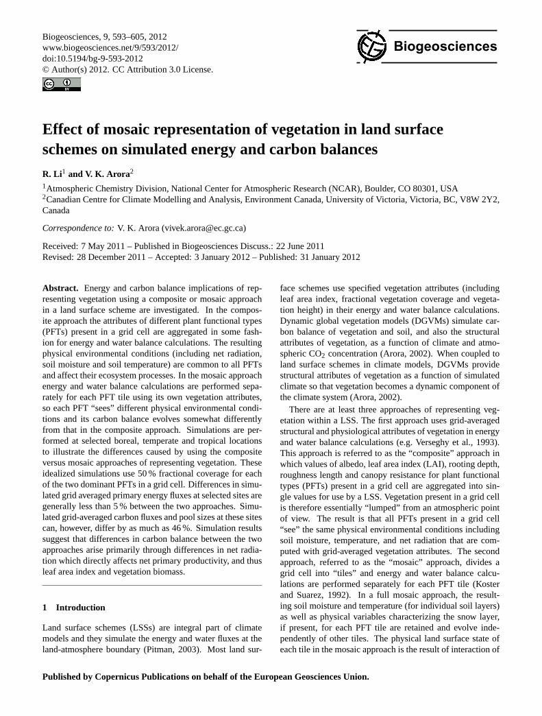
Fig. 2. Simulated daily average values of(a) net radiation,(b) latent heat flux and(c) sensible heat flux for the Manitoba location. The blueand the red lines represent grid-averaged values for the mosaic and composite approaches, respectively. The green and cyan lines representvalues for the evergreen needleleaf tree and C3 grass tiles in the mosaic approach, respectively. There are no PFT specific energy fluxes inthe composite approach. The table at the top summarizes the average annual values of the fluxes when using the two approaches.

from the standard data set used in CanESM1/2 based on theZobler (1986) soil data. In the mosaic approach same soildata are used for all tiles in a grid cell.

The 21 yr GOLD meteorological data are used repeat-edly at all locations until the simulated carbon pools comeinto equilibrium using both the composite and mosaic ap-proaches. Simulated primary energy and carbon balancequantities averaged over the last 21 yr are then compared be-tween the two approaches. In the next section, results are firstdiscussed for the two boreal sites followed by the temperateand tropical sites.

4 Results

4.1 The Manitoba and Siberia locations

Both boreal locations (Manitoba and Siberia) experiencecold sub-zero temperatures during winter which leads to pro-nounced seasonality in temperatures and the majority of theprecipitation occurs during summers (see Figs. S1 and S2 insupplementary information). The dominant PFTs are ever-green needleleaf trees and C3 grasses at the Manitoba loca-tion, and deciduous needleleaf trees and C3 grasses at theSiberia location.



26

1

2

3

Figure 3. Simulated daily average values of (a) soil temperature and (b) soil moisture for the 4

Siberia location. The blue and red lines represent grid-averaged values for the mosaic and 5

composite approaches, respectively. The green and cyan lines represent values for the 6

deciduous needleleaf tree and C3 grass mosaic tiles in the mosaic approach, respectively. 7

Grid averaged

Deciduous needleleaf trees

C3 grasses

Composite Mosaic

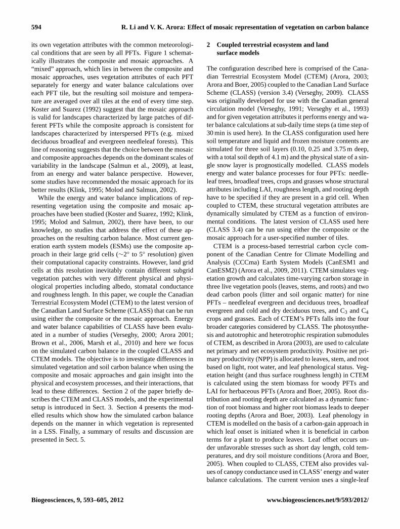
Fig. 3. Simulated daily average values of(a) soil temperature and(b) soil moisture for the Siberia location. The blue and red lines representgrid-averaged values for the mosaic and composite approaches, respectively. The green and cyan lines represent values for the deciduousneedleleaf tree and C3 grass mosaic tiles in the mosaic approach, respectively.

Energy fluxes

Figure 2 shows the simulated daily averaged values of netradiation, latent heat and sensible heat fluxes at the Man-itoba location. Plots are shown for individual PFT valuesin the mosaic approach as well as grid-averaged values forboth approaches. In the composite approach PFTs presentin a grid cell experience the same energy fluxes, which arecomputed using grid-averaged vegetation attributes, so thereare no PFT specific energy fluxes in the composite approach.The daily average net radiation in Fig. 2a shows a similar sea-sonal pattern for individual PFT tiles (green and cyan lines)in the mosaic approach as well as grid-averaged quantitiesobtained using the composite (red line) and mosaic (blueline) approaches since the driving downwelling radiation isthe same for all cases. The differences in grid-averaged netradiation between the composite (red line) and mosaic (blueline) approaches are small. However, there is a significantdifference between the net radiation flux for the individualPFT tiles in the mosaic approach and more so over the grow-ing season (about day 100 to 310 at the Manitoba locationbased on leaf onset and offset of C3 grasses, Fig. 4b). InFig. 2a, net radiation values (positive downward) are higherfor the evergreen needleleaf tree tile (green line) than for theC3 grass tile (cyan line) because of two reasons. First, thedarker needleleaf trees (albedo of 0.11) absorb more radia-tion than the brighter C3 grasses (albedo of 0.18). Second,the simulated surface temperature over the C3 grass tile is upto 4◦C higher during the summer season (not shown) whichincreases the outgoing longwave radiation. The higher tem-perature over the C3 grass tile is the result of its lower canopyheat capacity (because of lower vegetation biomass) as wellas lower LAI (which causes reduced shading) compared tothe needleleaf evergreen tree tile (Fig. 4b). In comparison,

both PFTs in the composite approach receive the same netradiation which is calculated using the grid-averaged albedoand surface temperature. The sharp increase in net radia-tion for C3 grasses around day 100 (∼10 April) in the mo-saic approach is the result of leaf onset for grasses (as shownin Fig. 4b) while the increase in net radiation for evergreenneedleleaf trees is more gradual and is primarily the resultof increase in downwelling radiation. Figures 2b and c showthat for the Manitoba location the composite approach yieldshigher grid-averaged latent heat flux (positive upward), es-pecially during summer (the red line is higher than the blueline), but similar sensible heat flux (positive upward) com-pared to the mosaic approach.

Qualitatively similar results are obtained for the Siberia lo-cation where the net radiation values are higher for the darkerdeciduous needleleaf trees than for the brighter C3 grasses(Table 1) in response to differences in albedo and tempera-ture (warmer temperatures over the C3 grass tile as seen inFig. 3a, which shows soil temperatures for the top 0.6 m atthe Siberia location). The difference between the two sites isthat while the needleleaf trees at the Manitoba location haveevergreen phenology they have deciduous phenology at theSiberia location. Compared to the composite approach, themosaic approach yields higher latent and sensible heat fluxesfor needleleaf trees at both locations and lower values for C3grasses, primarily in response to the differences in net radi-ation. The implication of differences in net radiation flux isthat in the composite approach the needleleaf trees receiveless and C3 grasses receive more radiation than in the mosaicapproach, at both locations. Since radiation is an importantdriver for vegetation growth these differences in net radiationhave significant impacts on the carbon balance, as discussedlater.



Mosaic approach Composite approach

Carbon quantities Grid-

averaged

Evergreen

needleleaf trees C3 grasses

Grid-

averaged

Evergreen


NPP (g C m−2

yr−1

) 234.1 355.0 113.3 316.8 292.5 341.1

Max. LAI (m2

m−2

) 1.8 2.8 0.9 2.3 2.4 2.2

Soil carbon mass

(Kg C m−2

) 6.1 7.0 5.2 8.9 5.5 12.2

Vegetation biomass

(Kg C m−2

) 2.5 4.9 0.2 2.1 3.7 0.6

Grid averaged

Evergreen needleleaf trees C3 grasses

Mosaic Composite

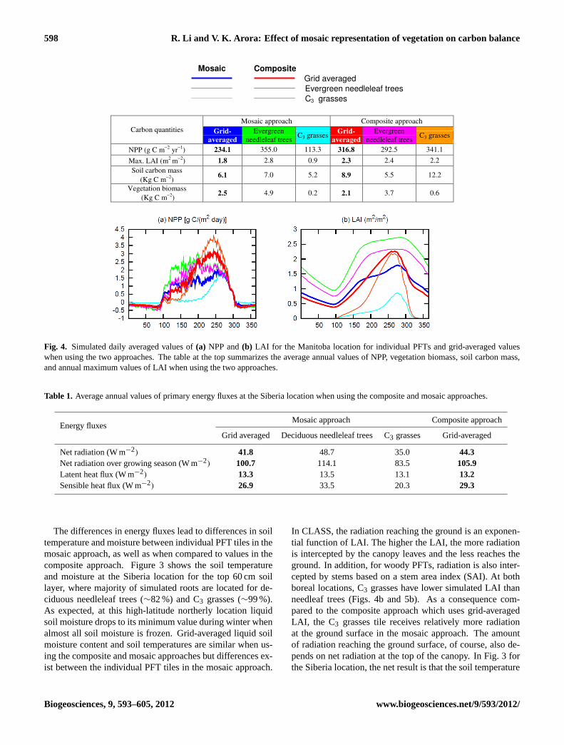
Fig. 4. Simulated daily averaged values of(a) NPP and(b) LAI for the Manitoba location for individual PFTs and grid-averaged valueswhen using the two approaches. The table at the top summarizes the average annual values of NPP, vegetation biomass, soil carbon mass,and annual maximum values of LAI when using the two approaches.

Table 1. Average annual values of primary energy fluxes at the Siberia location when using the composite and mosaic approaches.

Energy fluxesMosaic approach Composite approach

Grid averaged Deciduous needleleaf trees C3 grasses Grid-averaged

Net radiation (W m−2) 41.8 48.7 35.0 44.3Net radiation over growing season (W m−2) 100.7 114.1 83.5 105.9Latent heat flux (W m−2) 13.3 13.5 13.1 13.2Sensible heat flux (W m−2) 26.9 33.5 20.3 29.3

The differences in energy fluxes lead to differences in soiltemperature and moisture between individual PFT tiles in themosaic approach, as well as when compared to values in thecomposite approach. Figure 3 shows the soil temperatureand moisture at the Siberia location for the top 60 cm soillayer, where majority of simulated roots are located for de-ciduous needleleaf trees (∼82 %) and C3 grasses (∼99 %).As expected, at this high-latitude northerly location liquidsoil moisture drops to its minimum value during winter whenalmost all soil moisture is frozen. Grid-averaged liquid soilmoisture content and soil temperatures are similar when us-ing the composite and mosaic approaches but differences ex-ist between the individual PFT tiles in the mosaic approach.

In CLASS, the radiation reaching the ground is an exponen-tial function of LAI. The higher the LAI, the more radiationis intercepted by the canopy leaves and the less reaches theground. In addition, for woody PFTs, radiation is also inter-cepted by stems based on a stem area index (SAI). At bothboreal locations, C3 grasses have lower simulated LAI thanneedleaf trees (Figs. 4b and 5b). As a consequence com-pared to the composite approach which uses grid-averagedLAI, the C3 grasses tile receives relatively more radiationat the ground surface in the mosaic approach. The amountof radiation reaching the ground surface, of course, also de-pends on net radiation at the top of the canopy. In Fig. 3 forthe Siberia location, the net result is that the soil temperature



and moisture of the C3 grass (needleleaf deciduous tree) tilestarts to increase earlier (later) and are higher (lower) becauseof more (less) radiation reaching the ground surface in themosaic approach than the grid-averaged values in the com-posite approach. Qualitatively similar results are obtained atthe Manitoba location (not shown).

Carbon fluxes and pools

Figure 4 compares the daily averaged values of primary car-bon quantities (NPP, LAI, soil carbon mass and vegetationbiomass) from simulations using the composite and mosaicapproaches for the Manitoba location. Compared to Fig. 2,there are two additional lines in each panel, in magenta andorange colors, which represent PFT-specific carbon quanti-ties in the composite approach. While grid-averaged vege-tation attributes are used for energy and water balance cal-culations in the composite approach by CLASS, CTEM stillcalculates all terrestrial ecosystem processes separately forthe PFTs present in a grid cell albeit using same physical en-vironmental conditions, as illustrated in Fig. 1.

Figure 4 shows large differences between carbon quan-tities when simulated using the composite and mosaic ap-proaches for the Manitoba location. All quantities are higherfor C3 grasses and lower for evergreen needleleaf trees inthe composite approach compared to the mosaic approach.In Fig. 4a, NPP of evergreen needleleaf trees is lower inthe composite approach (magenta line below the green line)because evergreen needleleaf trees receive lower net radia-tion than in the mosaic approach, as mentioned earlier (seeFig. 2a). In contrast, the productivity of C3 grasses is higherin the composite approach (orange line above the cyan line)than in the mosaic approach because they receive higher netradiation in the composite approach. These differences inNPP lead to differences in simulated LAI, soil carbon massand vegetation biomass (summarized in the table above thefigure). In Fig. 4b, CTEM simulates the seasonality of leafarea indices for both PFTs realistically at the Manitoba loca-tion, but some limitations remain. Evergreen needleleaf treesretain leaves throughout the year but the simulated seasonalvariability is likely too large. C3 grasses, as expected, are ac-tive during summer and dormant during winter but the LAIpeaks towards the end of the growing season and not duringthe middle of the growing season as is generally observed.

Figure 4b shows that absolute values of LAI are differentbetween the two approaches with evergreen needleleaf treesexhibiting lower LAI and the C3 grasses showing more thandoubling of maximum annual LAI in the composite approachcompared to the mosaic approach. The increased LAI for C3grasses in the composite approach is the result of higher NPPdue to higher net radiation received by C3 grasses. The ta-ble in Fig. 4 shows that the use of the composite approachat the Manitoba location significantly increases soil carbonmass for C3 grasses by∼135 %. In contrast, the simulatedsoil carbon mass for needleleaf trees is slightly lower in the

composite approach than in the mosaic approach. While allother grid-averaged carbon quantities are higher in the com-posite approach it yields slightly lower grid averaged vege-tation biomass than in the mosaic approach (Fig. 4). This isbecause the decrease in the vegetation biomass for evergreenneedleleaf trees in the composite approach, due to lower netradiation, is not compensated by increase in the vegetationbiomass of C3 grasses, which receive higher radiation in thecomposite approach. Grasses do not include the woody stemcomponent and thus for the same NPP they yield lower veg-etation biomass but higher soil carbon mass because of theirlower soil decomposition rates compared to woody PFTs(Guo and Gifford, 2002; Jackson et al., 2002; Arora andBoer, 2010). Overall at the Manitoba location, net radia-tion is the primary driver of differences in the carbon balancebetween the two approaches. Grid-averaged NPP and soilcarbon mass are up to 46 % higher, but grid-averaged vege-tation biomass is slightly lower, in the composite approachcompared to the mosaic approach.

Figure 5 compares the daily averaged values of primarycarbon quantities for the Siberia location. The growing sea-son is short for both C3 grasses and deciduous needleleaftrees at this high-latitude location. Both PFTs start to growin late spring (indicated by positive NPP and leaf onset inFig. 5a and b, respectively) when the favourable weather ar-rives and become dormant in early fall when physical envi-ronmental conditions become unfavourable. NPP, LAI andvegetation biomass (Table in Fig. 5) are all higher for bothdeciduous needleleaf trees and C3 grasses in the compositeapproach compared to the mosaic approach. This behaviouris in contrast to the Manitoba location, where these carbonquantities were smaller for the evergreen needleleaf trees andlarger for C3 grasses in the composite compared to the mo-saic approach, primarily in response to the lower and highernet radiation these PFTs received. For the Siberia location,NPP, LAI and vegetation biomass are higher for C3 grassesin the composite approach compared to the mosaic approachbecause the higher net radiation (Table 1) more than com-pensates for the slightly lower soil moisture (Fig. 3b). TheNPP of deciduous needleleaf trees is slightly higher in thecomposite approach despite lower net radiation (Table 1),whose effect is overcome by an early leaf onset (∼9 days)(Fig. 5b) associated with early availability of liquid soilmoisture (Fig. 3b), compared to the mosaic approach. InCTEM, leaf onset is initiated when net photosynthesis forleaves (photosynthesis minus leaf respiration) remains pos-itive for seven consecutive days and PFT-specific environ-mental constraints are also relieved (Arora and Boer, 2005).Early availability of liquid soil moisture implies that the for-mer condition is met earlier in the composite approach lead-ing to higher NPP, LAI and vegetation biomass.

Values of soil carbon, which depend on NPP as well asrespiration from the soil carbon pool, behave somewhat dif-ferently than vegetation biomass. Higher values of NPPincrease soil carbon and higher values of temperature and




Carbon quantities

Grid-

averaged

Deciduous


Grid-

averaged

Deciduous


NPP (g C m−2

yr−1

) 138.0 152.8 123.3 186.2 195.7 176.7

Max. LAI (m2

m−2

) 1.2 1.8 0.6 1.5 2.2 0.9

Soil carbon mass (Kg C m−2

) 14.9 17.6 12.2 16.1 16.2 16.0

Vegetation biomass (Kg C m−2

) 1.3 2.4 0.2 1.7 3.1 0.3

Grid averaged

Deciduous needleleaf trees C3 grasses

Mosaic Composite

Fig. 5. Simulated daily averaged values of(a) NPP and(b) LAI for the Siberia location for individual PFTs and grid-averaged values whenusing the two approaches. The table at the top summarizes the average annual values of NPP, vegetation biomass, soil carbon mass, andannual maximum values of LAI when using the two approaches.

favourable moisture conditions, which increase respiration,decrease soil carbon. Soil carbon values for C3 grasses arehigher in the composite approach compared to the mosaicapproach (Table in Fig. 5), in response to increase in NPP(Fig. 5a) as well as lower soil temperature (Fig. 3a). Soilcarbon values for deciduous needleleaf trees are lower in thecomposite compared to the mosaic approach despite higherNPP (Fig. 5a) because of the higher soil temperature (Fig. 3a)and moisture (Fig. 3b) which increase soil respiration andconsequently decrease the equilibrium value of soil carbon.

Unlike the Manitoba location where the differences in netradiation are the primary driver of differences in carbon bal-ance, at the Siberia location the differences in soil mois-ture (which initiates early leaf onset in the composite ap-proach for the deciduous needleleaf trees) also play an im-portant role. Differences in soil moisture between the twoapproaches become important at the Siberia location becauseof the deciduous phenology of needleleaf trees at this lo-cation compared to their evergreen phenology at the Man-itoba location. Overall, at the Siberia location, differencesin net radiation, soil moisture and soil temperature and theirinteractions with various ecosystem processes between thetwo approaches all contribute to differences in the simulatedcarbon balance between the two approaches yielding 35 %higher NPP, 8 % higher soil carbon mass and 31 % highervegetation biomass in the composite approach.

4.2 The Eastern United States location

The Eastern United States location shows less pronouncedseasonality in temperature compared to the two boreal loca-tions and precipitation is more or less uniformly distributedover the year (see Fig. S3 in supplementary information).The two dominant PFTs at this location are broadleaf colddeciduous trees and C3 crops. The broadleaf cold deciduoustrees with their lower albedo (albedo of 0.17) are characteris-tically darker than the C3 crops (albedo of 0.20). The differ-ence in the albedos of cold deciduous broadleaf trees and C3crops at this location is smaller than the difference in albe-dos of needleleaf trees and C3 grasses at the Manitoba andSiberia locations.

Table 2 compares the energy fluxes at this location ob-tained using the two approaches. The differences in grid av-eraged net radiation, latent and sensible heat fluxes betweenthe two approaches are small and around 3–5 %. The netradiation fluxes for the individual PFTs, however, differ con-siderably in the mosaic approach with higher differences overthe growing season (determined using seasonality of LAI)because of the differences in their albedos. The brighter C3crops receive less and the darker broadleaf trees receive moreradiation in the mosaic approach than in the composite ap-proach (which uses grid-averaged albedo).



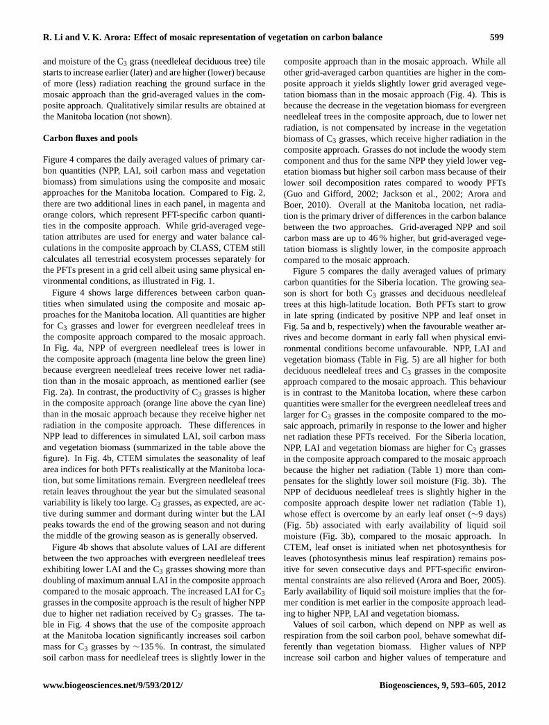
Table 2. Average annual values of primary energy fluxes at the Eastern United States location when using the composite and mosaicapproaches.


Grid averaged Cold deciduous broadleaf trees C3 crops Grid-averaged

Net radiation (W m−2) 59.3 66.1 53.3 61.8Net radiation over growing season (W m−2) 93.5 101.0 86.1 97.9Latent heat flux (W m−2) 34.5 37.9 31.6 36.3Sensible heat flux (W m−2) 23.2 26.5 20.2 23.9

Mosaic approach Composite approach Carbon quantities Grid-

averaged

Cold deciduous

broadleaf trees C3 crops

Grid-

averaged

Cold deciduous

broadleaf trees C3 crops

NPP (g C m−2

yr−1

) 481.2 695.3 292.8 679.0 642.7 712.9

Max. LAI (m2

m−2

) 2.4 3.9 1.3 3.3 3.8 2.8


) 7.4 12.5 3.0 9.3 11.3 7.6


) 3.6 7.6 0.05 3.5 7.3 0.13

Grid averaged

Cold deciduous broadleaf trees C3 crops

Mosaic Composite

Fig. 6. Simulated daily averaged values of(a) NPP and(b) LAI for the Eastern US location for individual PFTs and grid-averaged valueswhen using the two approaches. The table at the top summarizes the average annual values of NPP, vegetation biomass, soil carbon mass,and annual maximum values of LAI when using the two approaches.

Similar to the Manitoba location, the differences in net ra-diation are the primary driver of differences in carbon bal-ance between the two approaches (Fig. 6). The NPP andLAI of C3 crops more than doubles in the composite ap-proach resulting in 41 % higher grid-averaged NPP and 26 %higher grid-averaged soil carbon. The vegetation biomassof C3 crops remains small in both approaches because cropsare harvested at the end of their growing season and there-fore do not contribute much to the grid averaged vegetationbiomass (see table at the top in Fig. 6). The NPP and LAI ofcold deciduous broadleaf trees reduces in the composite ap-proach because of less radiation they receive resulting in theirlower vegetation and soil carbon mass. The changes in car-bon quantities are larger for C3 crops than for cold deciduous

broadleaf trees because of their larger percentage differencein net radiation between the two approaches. Overall, at thislocation the use of the composite approach leads to highergrid-averaged NPP, LAI and soil carbon mass.

4.3 The Africa location

The daily average temperature at the location in Africa hasthe least pronounced seasonal cycle of all locations (seeFig. S4 in supplementary information). This tropical site ex-periences an approximately 60–70 day long dry season withmost precipitation falling from late February to early Novem-ber.



30

1

2

3

4

5

Figure 7. Simulated daily average values of (a) soil temperature and (b) soil moisture for the 6

Africa location. The blue and red lines represent grid-averaged values for the mosaic and 7

composite approaches, respectively. The green and cyan lines represent values for the 8

evergreen broadleaf tree and dry deciduous broadleaf tree mosaic tiles in the mosaic 9

approach, respectively. 10

Grid averaged

Evergreen broadleaf trees

Dry deciduous broadleaf trees

Mosaic Composite

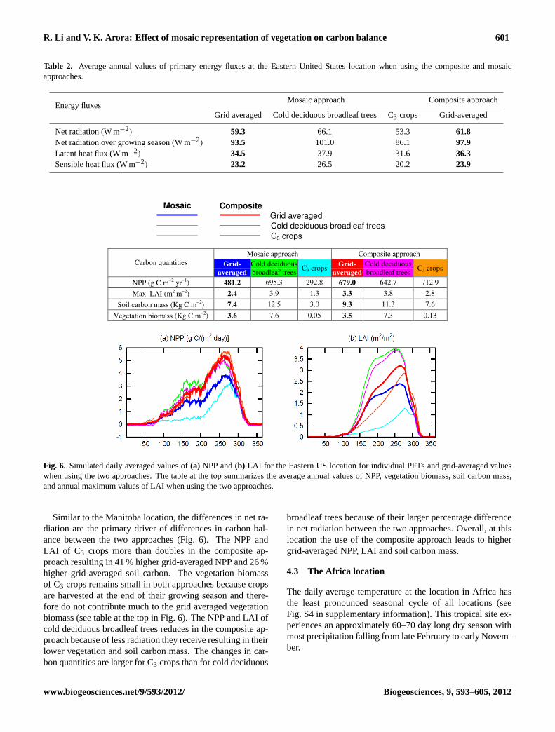
Fig. 7. Simulated daily average values of(a) soil temperature and(b) soil moisture for the Africa location. The blue and red lines representgrid-averaged values for the mosaic and composite approaches, respectively. The green and cyan lines represent values for the evergreenbroadleaf tree and dry deciduous broadleaf tree mosaic tiles in the mosaic approach, respectively.


Carbon quantities Grid-

averaged

Evergreen

broadleaf trees

Dry deciduous

broadleaf trees Grid-

averaged

Evergreen

broadleaf trees

Dry deciduous

broadleaf trees

NPP (g C m−2

yr−1

) 1233.3 1157.6 1308.9 1248.7 1138.4 1359.1

Max. LAI (m2

m−2

) 7.3 7.0 7.6 7.4 6.9 7.9


) 12.3 12.0 12.7 12.5 11.8 13.3


) 17.4 20.8 14.0 17.5 20.3 14.7

Grid averaged

Evergreen needleleaf trees Dry deciduous broadleaf trees

Mosaic Composite

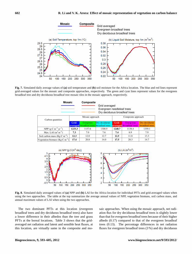
Fig. 8. Simulated daily averaged values of(a) NPP and(b) LAI for the Africa location for individual PFTs and grid-averaged values whenusing the two approaches. The table at the top summarizes the average annual values of NPP, vegetation biomass, soil carbon mass, andannual maximum values of LAI when using the two approaches.

The two dominant PFTs at this location (evergreenbroadleaf trees and dry deciduous broadleaf trees) also havea lower difference in their albedos than the tree and grassPFTs at the boreal locations. Table 3 shows that the grid-averaged net radiation and latent and sensible heat fluxes, atthis location, are virtually same in the composite and mo-

saic approaches. When using the mosaic approach, net radi-ation flux for dry deciduous broadleaf trees is slightly lowerthan that for evergreen broadleaf trees because of their higheralbedo (0.17) compared to that of the evergreen broadleaftrees (0.13). The percentage differences in net radiationfluxes for evergreen broadleaf trees (3 %) and dry deciduous



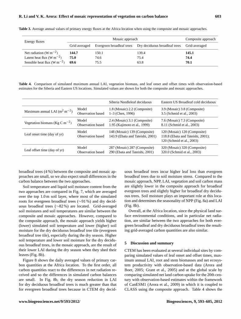
Table 3. Average annual values of primary energy fluxes at the Africa location when using the composite and mosaic approaches.


Grid averaged Evergreen broadleaf trees Dry deciduous broadleaf trees Grid-averaged

Net radiation (W m−2) 144.7 150.1 139.4 145.1Latent heat flux (W m−2) 75.0 74.6 75.4 74.4Sensible heat flux (W m−2) 69.6 75.5 63.8 70.1

Table 4. Comparison of simulated maximum annual LAI, vegetation biomass, and leaf onset and offset times with observation-basedestimates for the Siberia and Eastern US locations. Simulated values are shown for both the composite and mosaic approaches.

Siberia Needleleaf deciduous Eastern US Broadleaf cold deciduous

Maximum annual LAI (m2 m−2)Model 1.8 (Mosaic) 2.2 (Composite) 3.9 (Mosaic) 3.8 (Composite)Observation based 1–3 (Chen, 1996) 3.5 (Schmid et al., 2003)

Vegetation biomass (Kg C m−2)Model 2.4 (Mosaic) 3.1 (Composite) 7.6 (Mosaic) 7.3 (Composite)Observation based 1.95 (Kajimoto et al., 1999) 8.11 (Schmid et al., 2003)

Leaf onset time (day of yr)Model 148 (Mosaic) 139 (Composite) 120 (Mosaic) 120 (Composite)Observation based 143.9 (Ebata and Tateishi, 2001) 118.8 (Ebata and Tateishi, 2001);

120 (Schmid et al., 2003)

Leaf offset time (day of yr)Model 287 (Mosaic) 287 (Composite) 320 (Mosaic) 320 (Composite)Observation based 290 (Ebata and Tateishi, 2001) 320.0 (Schmid et al., 2003)

broadleaf trees (4 %) between the composite and mosaic ap-proaches are small, so we also expect small differences in thecarbon balance between the two approaches.

Soil temperature and liquid soil moisture content from thetwo approaches are compared in Fig. 7, which are averagedover the top 1.0 m soil layer, where most of the simulatedroots for evergreen broadleaf trees (∼91 %) and dry decid-uous broadleaf trees (∼82 %) are located. Grid-averagedsoil moistures and soil temperatures are similar between thecomposite and mosaic approaches. However, compared tothe composite approach, the mosaic approach yields higher(lower) simulated soil temperature and lower (higher) soilmoisture for the dry deciduous broadleaf tree tile (evergreenbroadleaf tree tile), especially during the dry season. Highersoil temperature and lower soil moisture for the dry decidu-ous broadleaf trees, in the mosaic approach, are the result oftheir lower LAI during the dry season when they shed theirleaves (Fig. 8b).

Figure 8 shows the daily averaged values of primary car-bon quantities at the Africa location. To the first order, allcarbon quantities react to the differences in net radiation re-ceived and so the differences in simulated carbon balancesare small. In Fig. 8b, the dry season reduction in LAIfor dry deciduous broadleaf trees is much greater than thatfor evergreen broadleaf trees because in CTEM dry decid-

uous broadleaf trees incur higher leaf loss than evergreenbroadleaf trees due to soil moisture stress. Compared to themosaic approach, NPP, LAI, vegetation and soil carbon massare slightly lower in the composite approach for broadleafevergreen trees and slightly higher for broadleaf dry decidu-ous trees. Soil moisture plays an important role at this loca-tion and determines the seasonality of NPP (Fig. 8a) and LAI(Fig. 8b).

Overall, at the Africa location, since the physical land sur-face environmental conditions, and in particular net radia-tion, are similar between the two approaches for both ever-green broadleaf and dry deciduous broadleaf trees the result-ing grid-averaged carbon quantities are also similar.

5 Discussion and summary

CTEM has been evaluated at several individual sites by com-paring simulated values of leaf onset and offset times, max-imum annual LAI, root and stem biomasses and net ecosys-tem productivity with observation-based data (Arora andBoer, 2005; Grant et al., 2005) and at the global scale bycomparing simulated net land carbon uptake for the 20th cen-tury with observation-based estimates within the frameworkof CanESM1 (Arora et al., 2009) in which it is coupled toCLASS using the composite approach. Table 4 shows the



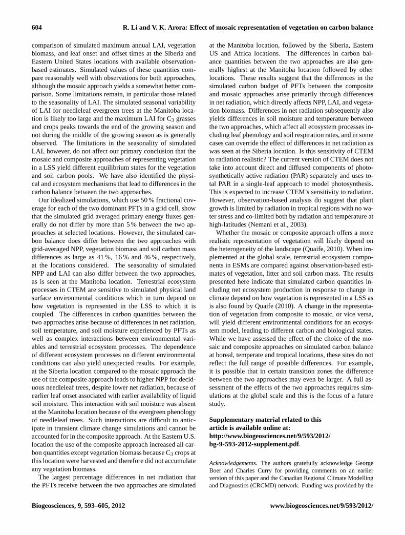
comparison of simulated maximum annual LAI, vegetationbiomass, and leaf onset and offset times at the Siberia andEastern United States locations with available observation-based estimates. Simulated values of these quantities com-pare reasonably well with observations for both approaches,although the mosaic approach yields a somewhat better com-parison. Some limitations remain, in particular those relatedto the seasonality of LAI. The simulated seasonal variabilityof LAI for needleleaf evergreen trees at the Manitoba loca-tion is likely too large and the maximum LAI for C3 grassesand crops peaks towards the end of the growing season andnot during the middle of the growing season as is generallyobserved. The limitations in the seasonality of simulatedLAI, however, do not affect our primary conclusion that themosaic and composite approaches of representing vegetationin a LSS yield different equilibrium states for the vegetationand soil carbon pools. We have also identified the physi-cal and ecosystem mechanisms that lead to differences in thecarbon balance between the two approaches.

Our idealized simulations, which use 50 % fractional cov-erage for each of the two dominant PFTs in a grid cell, showthat the simulated grid averaged primary energy fluxes gen-erally do not differ by more than 5 % between the two ap-proaches at selected locations. However, the simulated car-bon balance does differ between the two approaches withgrid-averaged NPP, vegetation biomass and soil carbon massdifferences as large as 41 %, 16 % and 46 %, respectively,at the locations considered. The seasonality of simulatedNPP and LAI can also differ between the two approaches,as is seen at the Manitoba location. Terrestrial ecosystemprocesses in CTEM are sensitive to simulated physical landsurface environmental conditions which in turn depend onhow vegetation is represented in the LSS to which it iscoupled. The differences in carbon quantities between thetwo approaches arise because of differences in net radiation,soil temperature, and soil moisture experienced by PFTs aswell as complex interactions between environmental vari-ables and terrestrial ecosystem processes. The dependenceof different ecosystem processes on different environmentalconditions can also yield unexpected results. For example,at the Siberia location compared to the mosaic approach theuse of the composite approach leads to higher NPP for decid-uous needleleaf trees, despite lower net radiation, because ofearlier leaf onset associated with earlier availability of liquidsoil moisture. This interaction with soil moisture was absentat the Manitoba location because of the evergreen phenologyof needleleaf trees. Such interactions are difficult to antic-ipate in transient climate change simulations and cannot beaccounted for in the composite approach. At the Eastern U.S.location the use of the composite approach increased all car-bon quantities except vegetation biomass because C3 crops atthis location were harvested and therefore did not accumulateany vegetation biomass.

The largest percentage differences in net radiation thatthe PFTs receive between the two approaches are simulated

at the Manitoba location, followed by the Siberia, EasternUS and Africa locations. The differences in carbon bal-ance quantities between the two approaches are also gen-erally highest at the Manitoba location followed by otherlocations. These results suggest that the differences in thesimulated carbon budget of PFTs between the compositeand mosaic approaches arise primarily through differencesin net radiation, which directly affects NPP, LAI, and vegeta-tion biomass. Differences in net radiation subsequently alsoyields differences in soil moisture and temperature betweenthe two approaches, which affect all ecosystem processes in-cluding leaf phenology and soil respiration rates, and in somecases can override the effect of differences in net radiation aswas seen at the Siberia location. Is this sensitivity of CTEMto radiation realistic? The current version of CTEM does nottake into account direct and diffused components of photo-synthetically active radiation (PAR) separately and uses to-tal PAR in a single-leaf approach to model photosynthesis.This is expected to increase CTEM’s sensitivity to radiation.However, observation-based analysis do suggest that plantgrowth is limited by radiation in tropical regions with no wa-ter stress and co-limited both by radiation and temperature athigh-latitudes (Nemani et al., 2003).

Whether the mosaic or composite approach offers a morerealistic representation of vegetation will likely depend onthe heterogeneity of the landscape (Quaife, 2010). When im-plemented at the global scale, terrestrial ecosystem compo-nents in ESMs are compared against observation-based esti-mates of vegetation, litter and soil carbon mass. The resultspresented here indicate that simulated carbon quantities in-cluding net ecosystem production in response to change inclimate depend on how vegetation is represented in a LSS asis also found by Quaife (2010). A change in the representa-tion of vegetation from composite to mosaic, or vice versa,will yield different environmental conditions for an ecosys-tem model, leading to different carbon and biological states.While we have assessed the effect of the choice of the mo-saic and composite approaches on simulated carbon balanceat boreal, temperate and tropical locations, these sites do notreflect the full range of possible differences. For example,it is possible that in certain transition zones the differencebetween the two approaches may even be larger. A full as-sessment of the effects of the two approaches requires sim-ulations at the global scale and this is the focus of a futurestudy.

Supplementary material related to thisarticle is available online at:http://www.biogeosciences.net/9/593/2012/bg-9-593-2012-supplement.pdf.

Acknowledgements.The authors gratefully acknowledge GeorgeBoer and Charles Curry for providing comments on an earlierversion of this paper and the Canadian Regional Climate Modellingand Diagnostics (CRCMD) network. Funding was provided by the


http://www.biogeosciences.net/9/593/2012/bg-9-593-2012-supplement.pdf

http://www.biogeosciences.net/9/593/2012/bg-9-593-2012-supplement.pdf


Canadian Foundation for Climate and Atmospheric Sciences (CF-CAS) through support to the CRCMD network. We also thankthe two anonymous reviewers for their helpful comments and thecoordinating editor Victor Brovkin for his help and the opportunityto revise our manuscript.

Edited by: V. Brovkin

References

Arora, V. K.: Assessment of simulated water balance forcontinental-scale river basins in an AMIP 2 simulation, J. Geo-phys. Res. -Atmos., 106, 14827–14842, 2001.

Arora, V. K.: Modelling vegetation as a dynamic componentin soil-vegetation-atmosphere-transfer schemes and hydrologicalmodels, Rev. Geophys., 40, 1006,doi:10.1029/2001RG000103,2002.

Arora, V. K.: Simulating energy and carbon fluxes over winterwheat using coupled land surface and terrestrial ecosystem mod-els, Agr. Forest Meteorol., 118, 21–47, 2003.

Arora, V. K. and Boer, G. J.: A representation of variable root distri-bution in dynamic vegetation models, Earth Interact., 7, 6, 2003.

Arora, V. K. and Boer, G. J.: A parameterization of leaf phenologyfor the terrestrial ecosystem component of climate models, Glob.Change Biol., 11, 39–59, 2005.

Arora, V. K. and Boer, G. J.: Uncertainties in the 20th century car-bon budget associated with land use change, Glob. Change Biol.,16, 3327–3348, 2010.

Arora, V. K., Boer, G. J., Christian, J. R., Curry, C. L., Denman,K. L., Zahariev, K., Flato, G. M., Scinocca, J. F., Merryfield, W.J., and Lee, W. G.: The effect of terrestrial photosynthesis downregulation on the twentieth-century carbon budget simulated withthe CCCma Earth System Model, J. Climate, 22, 6066–6088,2009.

Arora, V. K., Scinocca, J. F., Boer, G. J., Christian, J. R., Denman,K. L., Flato, G. M., Kharin, V. V., Lee, W. G., and Merryfield, W.J.: Carbon emission limits required to satisfy future representa-tive concentration pathways of greenhouse gases, Geophys. Res.Lett., 38, L05805,doi:10.1029/2010GL046270, 2011.

Brown, R., Bartlett, P., MacKay, M., and Verseghy, D.: Evaluationof snow cover in CLASS for SnowMIP, Atmos.-Ocean, 44, 223–238, 2006.

Chen, J. M.: Optically-based methods for measuring seasonal vari-ation of leaf area index in boreal conifer stands, Agr. Forest Me-teorol., 80, 135–163, 1996.

Dirmeyer, P. and Tan, L.: A multi-decadal global land-surfacedata set of state variables and fluxes. COLA Technical ReportNo. 102, Centre for Ocean-Land-Atmosphere Studies, Calver-ton, Maryland, USA, 43 pp., 2001.

Ebata, M. and Tateishi, R.: Phenological stage monitoring in Siberiausing NOAA/AVHRR data, in: Proceedings of the ACRS 2001– 22nd Asian Conference on Remote Sensing, 5–9 November2001, Singapore, 412–417, 2001.

Grant, R. F., Arain, A., Arora, V., Barr, A., Black, T. A., Chen,J., Wang, S., Yuan, F., and Zhang, Y.: Intercomparison of tech-niques to model high temperature effects on CO2 and energy ex-change in temperate and boreal coniferous forests, Ecol. Model.,188, 217–252, 2005.

Guo, L. and Gifford, R.: Soil carbon stocks and land use change: ameta analysis, Global Change Biol., 8, 345–360, 2002.

Jackson, R., Banner, J., Jobbagy, E., Pockman, W., and Wall, D.:Ecosystem carbon loss with woody plant invasion of grasslands,Nature, 418, 623–626, 2002.

Kajimoto, T., Matsuura, Y., Sofronov, M. A., Volokitina, A. V.,Mori, S., Osawa, A., and Abaimov, A. P.: Above- and below-ground biomass and net primary productivity of a Larix gmeliniistand near Tura, Central Siberia, Tree Physiol., 19, 815–822,1999.

Koster, R. D. and Suarez, M. J.: A comparative-analysis of 2 landsurface heterogeneity representations, J. Climate, 5, 1379–1390,1992.

Klink, K.: Surface aggregation and subgrid-scale climate, Int. J.Climatol., 15, 1219–1240, 1995.

Leuning, R.: A critical-appraisal of a combined stomatal-photosynthesis model for C-3 plants, Plant Cell Environ., 18,339–355, 1995.

Marsh, P., Bartlett, P., MacKay, M., Pohl, S., and Lantz, T.:Snowmelt energetics at a shrub tundra site in the western Cana-dian Arctic, Hydrol. Process.,10.1002/hyp.7786, 24, 3603–3620, 2010.

Molod, A. and Salmun, H.: A global assessment of the mosaic ap-proach to modeling land surface heterogeneity, J. Geophys. Res.-Atmos., 107, 4217,doi:10.1029/2001JD000588, 2002.

Nemani, R., Keeling, C., Hashimoto, H., Jolly, W., Piper, S., Tucker,C., Myneni, R., and Running, S.: Climate-driven increases inglobal terrestrial net primary production from 1982 to 1999, Sci-ence, 300, 1560–1563, 2003.

Quaife, T. L.: Impacts of scale and heterogeneity in dynamic globalvegetation models, abstract B11B-0353, presented at 2010 FallMeeting, AGU, San Francisco, Calif., 13–17 December 2010.

Salmun, H., Molod, A., Albrecht, J., and Santos, F.: Scales ofvariability of surface vegetation: calculation and implicationsfor climate models, J. Geophys. Res.-Biogeosci., 114, G02007,doi:10.1029/2008JG000762, 2009.

Schmid, H. P., Su, H. B., Vogel, C. S., and Curtis, P. S.: Ecosystem-atmosphere exchange of carbon dioxide over a mixed hardwoodforest in Northern Lower Michigan, J. Geophys. Res.-Atmos.,108, 4417,doi:10.1029/2002JD003011, 2003.

Verseghy, D. L.: CLASS – a Canadian land surface scheme forGCMs. 1. Soil model, Int. J. Climatol., 11, 111–133, 1991.

Verseghy, D. L.: The Canadian Land Surface Scheme (CLASS): Itshistory and future, Atmos.-Ocean, 38, 1–13, 2000.

Verseghy, D. L.: CLASS – The Canadian Land Surface Scheme(Version 3.4) Technical Documentation (Version 1.1), Environ-ment Canada, Climate Research Division, Science and Technol-ogy Branch, Downsview, Ontario, Canada, 2009.

Verseghy, D. L., McFarlane, N. A., and Lazare, M.: CLASS – aCanadian land surface scheme for GCMs. 2. Vegetation modeland coupled runs, Int. J. Climatol., 13, 347–370, 1993.

Wang, A., Price, D. T., and Arora, V.: Estimating changes in globalvegetation cover (1850–2100) for use in climate models, GlobalBiogeochem. Cy., 20, GB3028,doi:10.1029/2005GB002514,2006.

Zobler, L.: A World soil file for global climate modelling, NASATechnical Memorandum 87802, NASA Goddard Institute forSpace Studies, New York, USA, 1986.


http://dx.doi.org/10.1029/2001RG000103

http://dx.doi.org/10.1029/2010GL046270

http://dx.doi.org/10.1002/hyp.7786

http://dx.doi.org/10.1029/2001JD000588

http://dx.doi.org/10.1029/2008JG000762

http://dx.doi.org/10.1029/2002JD003011

http://dx.doi.org/10.1029/2005GB002514

effect of mosaic representation of vegetation in land surface schemes on simulated energy and

Documents