Eo

P1

2

a

ARRA

KEPESW

1

wiAFaetw

UT

(

0h

Agricultural and Forest Meteorology 178–179 (2013) 106–119

Contents lists available at SciVerse ScienceDirect

Agricultural and Forest Meteorology

journa l homepage: www.e lsev ier .com/ locate /agr formet

ffect of long-term water table manipulationn peatland evapotranspiration

.A. Moore1,∗, T.G. Pypker2, J.M. Waddington1

School of Geography and Earth Sciences, McMaster University, Hamilton, ON, CanadaSchool of Forest Resources and Environmental Science, Michigan Technological University, Houghton, MI, USA

r t i c l e i n f o

rticle history:eceived 14 August 2012eceived in revised form 18 April 2013ccepted 20 April 2013

eywords:ddy covarianceeatlandvapotranspirationurface resistanceater table

a b s t r a c t

Continuous measurements of ecosystem scale evapotranspiration (ET) were obtained using the eddycovariance method over the 2010 and 2011 growing seasons (May–September) at three adjacent peat-lands that have undergone long-term water table manipulation. The three (wet, dry and intermediate)sites represent peatlands along a hydrological gradient, with different average depths to water table(WTD) and different resulting vegetation and microform assemblages. The 2010 growing season waswarmer and wetter than normal, while 2011 conditions were near normal. The difference in maximumdaily ET values (95th percentiles) between sites were greater in 2010 (3.14 mm d−1–4.17 mm d−1) com-pared to 2011 (3.68 mm d−1–3.95 mm d−1), yielding cumulative growing season ET that followed the wetto dry gradient in both 2010 and 2011. Synoptic weather conditions (i.e. air temperature, vapour pres-sure deficit, and incoming solar radiation, etc.) could not explain differences in ET between sites due totheir proximity to one another. Peat surface wetness was more spatially homogeneous at the wet sitedue to small average microtopographic variations (0.15 m) compared to the intermediate (0.30 m) anddry (0.41 m) sites. Although average Bowen ratios were less than one at all three sites, greater surfacewetness and heating at the wettest site lead to differences in energy partitioning, with higher averageBowen ratios at the sites with a shallow average WTD. No significant relation between normalized ET

and WTD was found at any of the sites that were consistent across both study years. In addition, the lackof a relation between ET and near-surface moisture suggests that the unsaturated hydraulic conductivityand the boundary layer resistance created by the vascular canopy combined with low surface roughnesslimits evaporative losses from the peat surface. This study suggests that the low ET of a dry site com-pared to a wet site may be due to the impact of a long-term change in WTD on leaf area and the relative

tiona

distribution of plant func

. Introduction

While peatland ecosystems cover only approximately 3% of theorld’s total land surface (Gorham, 1991), peatlands can cover

n excess of 50% of the landscape in regions such as Northernlberta, the Hudson/James Bay Lowland (e.g. Tarnocai, 1984),enno-Scandinavia, and the West Siberian Plain (e.g. Paavalainennd Paivanen, 1995). In areas where peatlands are abundant, thesecosystems can have a significant impact on regional climate

hrough surface–atmosphere exchanges of mass and energy,here evapotranspiration (ET) is a large component of the water

∗ Corresponding author at: School of Geography and Earth Sciences, McMasterniversity, 1280 Main Street West, Hamilton, ON, Canada.el.: +1 905 525 9140x20113; fax: +1 905 546 0463.

E-mail addresses: moorepa6@mcmaster.ca, paul.moore82@gmail.comP.A. Moore).

168-1923/$ – see front matter © 2013 Elsevier B.V. All rights reserved.ttp://dx.doi.org/10.1016/j.agrformet.2013.04.013

l groups.© 2013 Elsevier B.V. All rights reserved.

balance across peatland types (Price and Maloney, 1994; Kellnerand Halldin, 2002).

Peatland ecosystems also represent a potential long-termimpact on future climate (Frolking. et al., 2011) through their rolein the global carbon cycle, where the oxidation and/or combus-tion of the large carbon pool stored in peatlands (e.g. Gorham,1991; Vasander and Kettunen, 2006; Turetsky et al., 2011) wouldrepresent a positive feedback to current climate forcings. Rapidand/or long-term persistent oxidation of peatland carbon storeshas been inferred from future climate scenario modelling studies(Ise et al., 2008) and from experimental manipulation where sitesare impacted by multiple disturbances, such as temperature changeand drainage (Strack and Waddington, 2007; Chivers et al., 2009;Huemmrich et al., 2010). However, to improve our understandingof the role of peatland surface–atmosphere interactions on regional

climate and the potential of peatlands to feedback on global climatechange, a greater level understanding on peatland surface energypartitioning and the controls on ET is required (Den Hartog et al.,1994; Kellner, 2001; Kettridge and Baird, 2006).

rest M

rldrodmTobegolrRa(labtrtt2daW

avvdwps1asiabLaCloisaita

aseoscecav

P.A. Moore et al. / Agricultural and Fo

Due to the wet conditions prevalent in many peatlands, pastesearch has sought to characterize simple metrics relating peat-and ET to open-water or equilibrium evaporation and water tableepth (WTD). Equilibrium evaporation is defined as the evapo-ation rate from an extensive, well watered surface where theverlying air mass has no saturation deficit (Monteith, 1981), andiffers from open-water evaporation since the effect of entrain-ent of air from above the convective boundary layer (Priestley and

aylor, 1972) is not taken into account. In general, peatlands evap-rate at or near the equilibrium level, similar to high productivityroadleaf forests in the boreal region, but less than open-watervaporation (Baldocchi et al., 2000; Humphreys et al., 2006), sug-esting a weak but important control of vapour pressure deficit (D)r water limitation. The relation between ET, and WTD for peat-ands in general is not straight forward as studies have shown aange of responses including a strong WTD relation (Lafleur andoulet, 1992), no significant effect of WTD (Paramentier et al., 2009nd Wu et al., 2010), and a moderate or threshold type responseLafleur et al., 2005). The control of ET by D in peatlands is simi-arly varied. In peatlands dominated by vascular vegetation havingrelatively high LAI, there is evidence that ET is strongly controlledy surface resistance (Comer et al., 1999), and thus by D. In con-rast, clear-day ET was shown to be more strongly controlled by netadiation in a moss-dominated peatland (Price, 1991). In assessinghe controls on ET, surface resistance has been shown to be bet-er correlated with D in comparison to water availability (Kellner,001). However, the strength of the relation between ET and D caneteriorate under drying conditions (Admiral et al., 2006), wherechange in the ET regime may only be detected at relatively largeTD (Lafleur et al., 2005).These findings suggest that the range of responses in peatland ET

re, in part, due to the disparate controls on moss evaporation andascular plant ET, and their respective links to the spatio-temporalariability in moisture availability. Moreover, the relative abun-ance of vascular vegetation within a given peatland will dictatehether a peatland can be modelled using a big-leaf model with ETartitioned into soil, vegetation, and interception loss componentsuch as in the ORCHIDEE land surface scheme (Ducoudre et al.,993), or if a more detailed dual source model is required (Kimnd Verma, 1996; Lafleur et al., 2005). The Canadian land surfacecheme (CLASS) and Community Land Model have recognized themportance of both organic soils (e.g. Letts et al., 2000; Lawrencend Slater, 2008) as well as the need for a dual source model toetter characterize surface evaporation (e.g. Verseghy et al., 1993;awrence et al., 2011). Nevertheless, despite having dual source ETnd organic soil parameterization, Comer et al. (1999) show thatLASS does not simulate ET well for peatlands with a sparse vascu-

ar canopy, suggesting a potential need for better parameterizationf moss evaporation. Furthermore, potentially important dynam-cs which are missing from peatland classifications in land surfacechemes include the role of microtopography on the spatial vari-bility in moisture (e.g. Wu et al., 2011) and plant functional groupsn peatlands (e.g. Korner et al., 1979), as well as the ability for micro-opography and plant functional groups to change through time asresult of changing environmental conditions.

The response of peatland ET to changes in moisture avail-bility has been characterized using interannual variability at aite (Lafleur et al., 2005; Liljedahl et al., 2011), climatic gradi-nts between sites (Humphreys et al., 2006), and through fieldr laboratory manipulations (Whittington and Price, 2006). Mea-urements in years with different synoptic weather conditionsan be used to quantify short-term, direct impacts on surface

nergy partitioning that result from warmer/colder or wetter/drieronditions (Teklemariam et al., 2010), but often both moisturevailability, temperature, and other synoptic weather variablesary simultaneously so specific impact attribution can be difficult to

eteorology 178–179 (2013) 106–119 107

elicit. Comparisons between sites along climatic gradients are oftenused to represent long-term impacts of climate (e.g. Chapin et al.,2000; Eugster et al., 2000), where plant community compositionis assumed to be in quasi-equilibrium with the local climate. How-ever, attribution of change can be confounded by other overlappinggradients (e.g. nitrogen deposition, Lund et al., 2009). Manipulationstudies, which are predominantly focused on carbon fluxes (e.g.Oechel et al., 1998; Weltzin et al., 2003; Strack and Waddington,2007; Chivers et al., 2009; Huemmrich et al., 2010), use warm-ing or draining to control for different anticipated climate changeeffects, but are often limited to a few years and thus are poten-tially measuring the response of a system in disequilibrium. Assuch, there is a need to characterize peatland ET following a per-sistent change in moisture availability, where sufficient time haselapsed for both peat hydrophysical properties and the vegetationcommunity to come into a quasi-equilibrium with the new hydro-logical conditions. In order to be able to constrain the degrees offreedom in a comparative study, the ideal research design wouldbe to examine impacted and control sites in close enough proximityto one another that they can be considered to be subjected to thesame synoptic weather conditions. To address this research needwe took advantage of a large scale ‘natural experiment’ resultingfrom the construction of berms perpendicular to water flow in alarge peatland complex in northern Michigan ca. 75 years ago bymeasuring growing season ET at three adjacent peatlands alonga post-disturbance hydrosequence using the eddy covariance (EC)method. The objectives of this study were to: (i) quantify ET alonga hydrosequence under the same synoptic weather conditions; (ii)determine if growing season ET was different between sites; and(iii) determine whether energy partitioning and/or controls on ETdiffered between sites.

2. Methods

2.1. Study site

The study area is located in the Seney National Wildlife Refuge(SNWR) in the Upper Peninsula of Michigan (46.20◦ N, 86.02◦ W,elev. ∼205 m.a.s.l.). The region is characterized by relatively flattopography which slopes towards the south-east at 1.1–2.3 m km−1

(Heinselman, 1965). Land cover consists primarily of upland forests(67%), and open peatlands (20%), while the remainder of the regionis made up of mostly forested swamps and open water (Casselman,2009). Wet sand of glacial origin overlies the regional bedrock up toa thickness of 60 m (Albert, 1995). Surface soils throughout SNWRare mostly a complex of poorly drained muck and sand, while thestudy area itself contains poorly drained peats (Casselman, 2009).

The peatland complex within SNWR is subdivided by a combina-tion of upland sand ridges of lacustrine origin, creeks, old drainageditches, as well as a network of roads and berms constructed mostlyduring the late 1930s and early 1940s by the Civilian Conserva-tion Corps (Kowalski and Wilcox, 2003; Wilcox et al., 2006) for thepurpose of creating open-water habitat for migratory birds. As aresult of the construction of berms perpendicular to water flow inthe study area ca. 75 years ago, a natural experiment was createdwhere an upslope peatland site (hereafter referred to as WET) likelybecame wetter and a downstream peatland site (hereafter referredto as DRY) likely became drier. Aerial photography of the study areashows a clear increase in ponding at the WET site and a rapid terres-trialization at the DRY site following berm construction. Moreover,contemporary WTD data shows a large difference between the WET

and DRY sites, with the latter being up to 50–60 cm deeper. A sitewith an intermediate WTD variation (hereafter referred to as INT)is located adjacent to the WET site. All three study sites are locatedin the southern portion of SNWR and have greater than 200 m of

1 rest M

caasm2

gmnvlbPtrp(ppsaoaap

3f5t

2

sdaaUuCbvasm

CaurmnctCtr1oI

wHt

08 P.A. Moore et al. / Agricultural and Fo

ontinuous fetch in the dominant wind sector, with only 100 mlong the lateral wind sectors. All three sites are located directlydjacent to one another along a roughly north–south transect, andeparated by sandy upland ridges between 25 and 100 m wide. Theaximum distance between tower-based measurements (Section

.2) is approximately 750 m.Dominant vegetation at all three peatland sites consists of a

round cover of Sphagnum sp. (S. angustifolium, S. capillifolium, S.agelanicum), with an overstory of vascular species. The domi-ant vascular vegetation consists of Carex oligosperma, Eriophorumaginatum, Ericaceae (e.g. Chamaedaphne calyculata, Ledum groen-andicum, Kalmia polifolia, and Vaccinium oxycoccus), with treesecoming more abundant at sites with increasing WTD (e.g.icea mariana, Pinus banksiana, and Larix laricina), particularlyowards the margins. The berm and upland area surrounding theesearch sites is dominated by coniferous species such as redine (Pinus resinosa), eastern white pine (Pinus strobus), jack pinePinus banksiana), and black spruce (Picea mariana). Although eacheatland site has almost identical species richness, the relativeroportion of given species differs between sites (J. Hribljan, per-onal communication). Generally, shrubs dominate hummocks,nd sedges dominate hollows across sites, where the proportionf hummocks, height of hummocks relative to adjacent hollows,nd acidity of near-surface water increases from the WET, to INTnd DRY sites (Table 1). Moreover, both leaf area index (LAI) andlant area index (PAI) are highest at the WET site (Table 1).

Based on the 1981–2010 climate normals from the NewberryS weather station (46.32◦ N, 85.50◦ W, elev. ∼260 m.a.s.l.) ∼45 kmrom the study sites, the area has an average annual temperature of.6 ◦C and receives 784 mm of precipitation, where greater monthlyotals occur during May through October (NOAA NCDC, 2012).

.2. Instrumentation

Standard EC equipment was used at all three sites to mea-ure surface energy and mass exchanges based on the methodescribed by Baldocchi et al. (1996). Three component wind speednd sonic air temperature were measured using a CSAT3 3D sonicnemometer-thermometer [Campbell Scientific Inc. (CS), Logan,T, USA]. Water vapour and CO2 concentrations were measuredsing an LI-7500A open-path infrared gas analyzer (IRGA) (LI-OR Biosciences, Lincoln, Nebraska). All EC sensors were mountedetween 1.7 and 2.1 m above the average hummock surface, had aertical and lateral separation less than 0.15 and 0.3 m, respectively,nd were oriented upwind of the tower based on the dominantummertime wind direction. EC data was sampled at 10 Hz, withean values and fluxes calculated every 30 min.Radiation measurements were made using a combination of

MP3 and LP02 pyranometers (CS), NR-LITE net radiometers (CS),nd CNR2 net short- and long-wave radiometers (CS). A CNR2 wassed at the INT and DRY site mounted at a height of 1.78 and 3.2 m,espectively, while a NR-LITE was used at the WET and INT siteounted at a height of 1.7 and 2.3 m, respectively. Both types of

et radiometers were used at the INT site to provide a continuousross-comparison of instrument type in order to correct for any sys-ematic bias. In order to calculate albedo for all three sites, a singleMP3 was mounted 1.7 m above the sedge canopy at the WET siteo measure incoming short-wave radiation. Outgoing short-waveadiation was measured at the WET site using a LP02 mounted at.7 m above the sedge canopy. Outgoing short-wave radiation wasbtained by difference from net shortwave radiation at each of theNT and DRY sites using a CNR2.

Supplementary air temperature and relative humidity (RH)ere measured and recorded at 10 Hz using a HMP45C (Vaisala Oyj,elsinki, Finland) temperature and RH probe mounted in a radia-

ion shield at a height of 1.35 m on all EC towers. Peat temperature

eteorology 178–179 (2013) 106–119

profiles were measured in a representative hummock and hollow ateach site using T-type thermocouple (Omega Engineering, CT, USA)wire inserted at depths of 0.01, 0.05, 0.1, 0.2, and 0.5 m relative tothe local surface.

Measured hydrometric data included rainfall, soil volumet-ric water content (�), and WTD. Rainfall was measured using aTE525 tipping bucket rain gauge (Texas Electronics, Dallas, TX, USA)mounted 0.7 m above the surface. Soil moisture profiles were mea-sured using CS-616 water content reflectometers (CS). � sensorswere installed at all three sites in a representative hummock andhollow at depths of 0.05, 0.15, and 0.25 m relative to the surface,with an additional sensor at 0.5 m in hummocks. WTD was mea-sured hourly in 1.5 m deep wells using self-logging LevelloggerJunior pressure transducers [Solinst, Georgetown, ON (Solinst)].WTD measurements were corrected for changes in atmosphericpressure using a Barologger Gold barometric logger (Solinst). WTDwas recorded at all three sites in two separate groundwater wellswith the average local topography used as a datum, where theheight of the average local surface was determined from 50 m tran-sects with the groundwater wells at the centre.

All high-frequency data was recorded on a CR5000 datalogger(CS) at the WET and DRY site, while a CR3000 datalogger (CS) wasused at the INT site. Meteorological, peat temperature and � datawere measured every minute and averaged and recorded at 30 minintervals using a CR1000 (CS) or CR10X (CS) datalogger.

2.3. High-frequency data processing and corrections

Prior to calculating half-hour covariances, high-frequency ECmeasurements were subjected to a spike detection algorithm anal-ogous to that presented in Vickers and Mahrt (1997), where spikeswere identified when a measurement exceeded the recursive meanby a standard deviation of 2.6 (also derived recursively). The meanwas constructed as a recursive digital filter (Kaimal and Finnigan,1994):

c̃t =(

1 − �t

�f

)c̃t−1 + �t

�fct (1)

where ct is the measured value at time t, �t is the incrementaltime step between measurements (0.1 s), and �f is the RC filter timeconstant (60 s). The cut-off for spike detection is lower than thetypical 3–5 SD range reported by others (e.g. Baldocchi et al., 1997;Vickers and Mahrt, 1997; Humphreys et al., 2006) because, giventhe above time constant, the recursive mean is more responsive tocoherent transient departures from the long-term mean comparedto block averaging.

Sonic anemometer wind vectors were mathematically rotatedbased on the tilt correction algorithms presented by Wilczak et al.(2001), also known as the planar fit method. The planar fit methodhelps to address the problem of over-rotation in sloping terrainassociated with the more commonly used method of Tanner andThurtell (1969) as outlined by Lee et al. (2004).

Before calculating energy and mass fluxes, a time lag wasintroduced into the appropriate mass or energy time series in orderto maximize the average covariance with the rotated vertical windspeed. In addition to flux loss that results from the asynchronyin the measured time series due to finite instrument processingtimes, spectral transfer functions were used to correct for high-frequency spectral losses that result from sensor separation, lineand volume averaging, and digital filtering. Frequency responsecorrections were calculated according to the analytical solutions

presented in Massman (2000) and applied to despiked, rotated, andlagged covariances.

Errors in EC flux measurements associated with variationsin air density due to changing temperature and humidity were

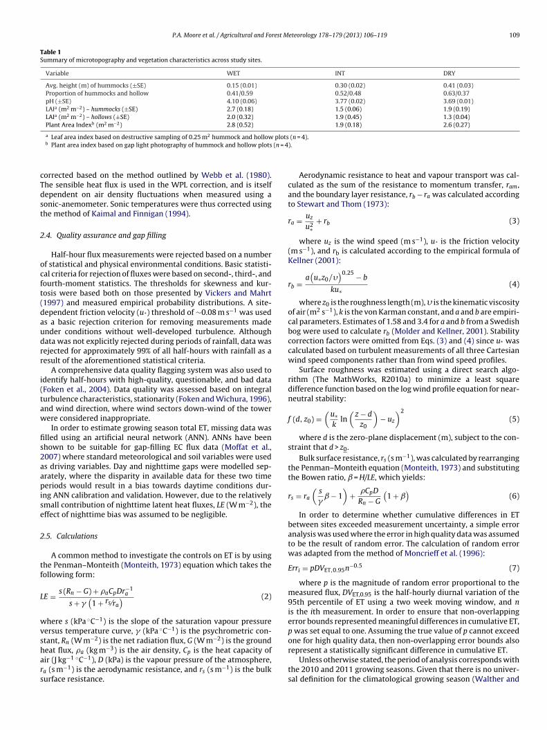
P.A. Moore et al. / Agricultural and Forest Meteorology 178–179 (2013) 106–119 109

Table 1Summary of microtopography and vegetation characteristics across study sites.

Variable WET INT DRY

Avg. height (m) of hummocks (±SE) 0.15 (0.01) 0.30 (0.02) 0.41 (0.03)Proportion of hummocks and hollow 0.41/0.59 0.52/0.48 0.63/0.37pH (±SE) 4.10 (0.06) 3.77 (0.02) 3.69 (0.01)LAIa (m2 m−2) – hummocks (±SE) 2.7 (0.18) 1.5 (0.06) 1.9 (0.19)LAIa (m2 m−2) – hollows (±SE) 2.0 (0.32) 1.9 (0.45) 1.3 (0.04)Plant Area Indexb (m2 m−2) 2.8 (0.52) 1.9 (0.18) 2.6 (0.27)

plots(n = 4

cTdst

2

ocft(daudrr

i(taw

fis2aapise

2

tf

L

wvshars

a Leaf area index based on destructive sampling of 0.25 m2 hummock and hollowb Plant area index based on gap light photography of hummock and hollow plots

orrected based on the method outlined by Webb et al. (1980).he sensible heat flux is used in the WPL correction, and is itselfependent on air density fluctuations when measured using aonic-anemometer. Sonic temperatures were thus corrected usinghe method of Kaimal and Finnigan (1994).

.4. Quality assurance and gap filling

Half-hour flux measurements were rejected based on a numberf statistical and physical environmental conditions. Basic statisti-al criteria for rejection of fluxes were based on second-, third-, andourth-moment statistics. The thresholds for skewness and kur-osis were based both on those presented by Vickers and Mahrt1997) and measured empirical probability distributions. A site-ependent friction velocity (u*) threshold of ∼0.08 m s−1 was useds a basic rejection criterion for removing measurements madender conditions without well-developed turbulence. Althoughata was not explicitly rejected during periods of rainfall, data wasejected for approximately 99% of all half-hours with rainfall as aesult of the aforementioned statistical criteria.

A comprehensive data quality flagging system was also used todentify half-hours with high-quality, questionable, and bad dataFoken et al., 2004). Data quality was assessed based on integralurbulence characteristics, stationarity (Foken and Wichura, 1996),nd wind direction, where wind sectors down-wind of the towerere considered inappropriate.

In order to estimate growing season total ET, missing data waslled using an artificial neural network (ANN). ANNs have beenhown to be suitable for gap-filling EC flux data (Moffat et al.,007) where standard meteorological and soil variables were useds driving variables. Day and nighttime gaps were modelled sep-rately, where the disparity in available data for these two timeeriods would result in a bias towards daytime conditions dur-

ng ANN calibration and validation. However, due to the relativelymall contribution of nighttime latent heat fluxes, LE (W m−2), theffect of nighttime bias was assumed to be negligible.

.5. Calculations

A common method to investigate the controls on ET is by usinghe Penman–Monteith (Monteith, 1973) equation which takes theollowing form:

E = s (Rn − G) + �aCpDr−1a

s + �(

1 + rs ⁄ra

) (2)

here s (kPa ◦C−1) is the slope of the saturation vapour pressureersus temperature curve, � (kPa ◦C−1) is the psychrometric con-tant, Rn (W m−2) is the net radiation flux, G (W m−2) is the ground

eat flux, �a (kg m−3) is the air density, Cp is the heat capacity ofir (J kg−1 ◦C−1), D (kPa) is the vapour pressure of the atmosphere,a (s m−1) is the aerodynamic resistance, and rs (s m−1) is the bulkurface resistance.

(n = 4).).

Aerodynamic resistance to heat and vapour transport was cal-culated as the sum of the resistance to momentum transfer, ram,and the boundary layer resistance, rb − ra was calculated accordingto Stewart and Thom (1973):

ra = uz

u2∗+ rb (3)

where uz is the wind speed (m s−1), u* is the friction velocity(m s−1), and rb is calculated according to the empirical formula ofKellner (2001):

rb =a(

u∗z0/�)0.25 − b

ku∗(4)

where z0 is the roughness length (m), � is the kinematic viscosityof air (m2 s−1), k is the von Karman constant, and a and b are empiri-cal parameters. Estimates of 1.58 and 3.4 for a and b from a Swedishbog were used to calculate rb (Molder and Kellner, 2001). Stabilitycorrection factors were omitted from Eqs. (3) and (4) since u* wascalculated based on turbulent measurements of all three Cartesianwind speed components rather than from wind speed profiles.

Surface roughness was estimated using a direct search algo-rithm (The MathWorks, R2010a) to minimize a least squaredifference function based on the log wind profile equation for near-neutral stability:

f (d, z0) =(

u∗k

ln(

z − d

z0

)− uz

)2

(5)

where d is the zero-plane displacement (m), subject to the con-straint that d > z0.

Bulk surface resistance, rs (s m−1), was calculated by rearrangingthe Penman–Monteith equation (Monteith, 1973) and substitutingthe Bowen ratio, ˇ = H/LE, which yields:

rs = ra

(s

�ˇ − 1

)+ �CpD

Rn − G

(1 + ˇ

)(6)

In order to determine whether cumulative differences in ETbetween sites exceeded measurement uncertainty, a simple erroranalysis was used where the error in high quality data was assumedto be the result of random error. The calculation of random errorwas adapted from the method of Moncrieff et al. (1996):

Erri = pDVET,0.95n−0.5 (7)

where p is the magnitude of random error proportional to themeasured flux, DVET,0.95 is the half-hourly diurnal variation of the95th percentile of ET using a two week moving window, and nis the ith measurement. In order to ensure that non-overlappingerror bounds represented meaningful differences in cumulative ET,p was set equal to one. Assuming the true value of p cannot exceedone for high quality data, then non-overlapping error bounds also

represent a statistically significant difference in cumulative ET.

Unless otherwise stated, the period of analysis corresponds withthe 2010 and 2011 growing seasons. Given that there is no univer-sal definition for the climatological growing season (Walther and

110 P.A. Moore et al. / Agricultural and Forest Meteorology 178–179 (2013) 106–119

120 150 180 210 240 270 300

0.6

0.4

0.2

0

−0.2

WT

D (

m)

120 150 180 210 240 270 300

20

40

60

Rai

nfal

l (m

m)

120 150 180 210 240 270 300

0.6

0.4

0.2

0

−0.2

DOY

WT

D (

m)

120 150 180 210 240 270 300

20

40

60

Rai

nfal

l (m

m)

120 150 180 210 240 270 300

0.2

0.4

0.6

0.8

1.0

θ (

m3 m

−3 )

WET

INT

DRY

120 150 180 210 240 270 300

0.2

0.4

0.6

0.8

1.0

DOY

θ (

m3 m

−3 )

b

c

a

d

2010

2011

F INT (df e hums

Ltc

tSl

3

3

bw(awDCgld

tsag2(i

f

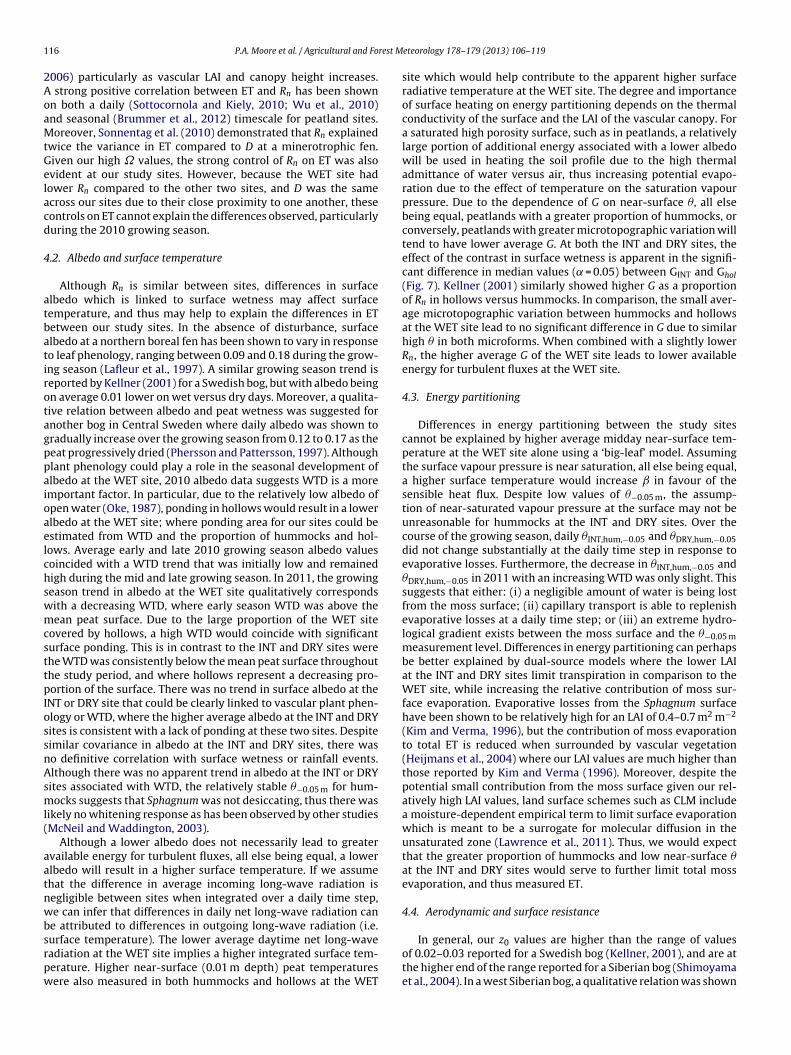
ig. 1. Daily total rainfall (bars) and water table levels (a and c) for the WET (solid),or clarity) at all three sites (b and d) measured at 0.05 m depth in a representativeasons.

inderholm, 2006), the growing season herein corresponds to theime of year when air temperature (Ta) was above 5 ◦C for over fiveonsecutive days (Frich et al., 2002).

Finally, all data processing, quality assurance, and statisticalests were done using MATLAB 7.8 (The MathWorks Inc., 2009).tatistical tests were considered significant when the p-value wasess than 0.01.

. Results

.1. Meteorological and hydrological conditions

The length and timing of the growing season was similar inoth years (Table 2). Over the course of the two study years, 2011as slightly warmer based on a comparison of cumulative GDD

Table 2). GDD for 2010 and 2011 were similar to the historicalverage of 1629 ◦C based on climate normals from the Newberryeather station (1981–2010 US Normals Data – National Climaticata Center – National Oceanic and Atmospheric Administration).onsidering GDD during the period defined by the climatologicalrowing season alone, the difference between years becomes neg-igible. Moreover, during this period, there were no strong seasonalepartures in Ta from the normal in either study year.

Rainfall during the 2010 and 2011 growing season was higherhan normal (430 mm) over the same period (Table 2). The greatereasonal rainfall total in 2010 was the result of both fewer dry daysnd greater average rainfall on wet days (Table 2). Despite a greaterrowing season rainfall total, there was an extended dry period in010 where there was a 22 day period with only 6.4 mm of rainfall

day of year (DOY) 130–151). The maximum period with no rainfalln 2010 and 2011 was 10 and 12 days, respectively.

The difference in the average WTD (Fig. 1) between sites wasairly consistent over 2010 (median: WTDWET − WTDINT = 0.20 m;

ash-dot), and DRY (dot) sites. Volumetric water content (three day average shownmock (grey) and hollow (black) over the 2010 (top) and 2011 (bottom) growing

and WTDWET − WTDDRY = 0.35 m) with the exception of someanomalous values where WTDWET was increasing whileWTDINT and WTDDRY were decreasing (DOY 266–273). Thedifference in average WTD was smaller in 2011 (median:WTDWET − WTDINT = 0.15 m; and WTDWET − WTDDRY = 0.28 m)where the magnitude of the difference between WTDWET andWTDDRY increased as WTDDRY moved into deeper peat late in thegrowing season. Overall, the average WTD was greater in 2011,which corresponds with a lower seasonal rainfall total. In terms ofseasonality, WT was relatively stable in 2010 except early in thegrowing season during the extended dry period (DOY 130–151).Conversely, 2011 was characterized by a shallow WTD early in thegrowing season with progressive drying due to fewer and smallerrainfall events.

The effect of WTD variation was not apparent in the near-surface(0.05 m) � of hummocks at two of the study sites (Fig. 1). Near-surface �INT,hum and �DRY,hum remained relatively stable throughoutthe growing season in both years, varying between 0.10 and0.20 m3 m−3. Both �WET,hum and all �hol had much greater ranges ofvariability in both years, loosely corresponding to periods of largeWTD variability. The magnitude of variability in �hol differs betweensites. During the drying phase of both study years, �hol reached aminimum daily value of 0.21 and 0.22 m3 m−3 at the WET site com-pared to 0.56 and 0.47 m3 m−3 for the INT site, and 0.73 m3 m−3

(2011 data missing) for the DRY site despite a greater WTD at theINT and DRY sites.

3.2. Surface energy exchange

3.2.1. EvapotranspirationDaily ET at the WET site had a maximum of 5.0 and 4.8 mm for

2010 and 2011, with typical (25th–75th percentile) values rangingfrom 1.9 to 3.4 mm d−1 and from 1.6 to 3.1 mm d−1 in each of the

P.A. Moore et al. / Agricultural and Forest Meteorology 178–179 (2013) 106–119 111

Table 2Summary of average climatological and flux variables for the study area.

Variable 2010 2011

Climatological growing season DOY: 136–306 DOY: 130–303GDDa (total/growing season) 1721 ◦C/1567 ◦C 1601 ◦C/1558 ◦CRainfall (total/dry days/avg. depth) 660 mm/96 days/8.2 mm 470 mm/112 days/7.1 mmTotal ET WET: 1.03 (417) WET: 0.93 (378)103 MJ m−2 (and mm) INT: 0.80 (323) INT: 0.84 (340)

DRY: 0.77 (314) DRY: 0.82 (336)Total Rn (±std. dev.b) WET: 1.70 (0.04) WET: 1.82 (0.05)103 MJ m−2 INT: 1.86 (0.04) INT: 1.92 (0.04)

DRY: 1.86 (0.04) DRY: 1.92 (0.05)Total G (±std. dev.b) WET: 0.076 (0.002) WET: 0.065 (0.008)103 MJ m−2 INT: 0.026 (0.002) INT: 0.021 (0.006)

DRY: 0.007 (0.001) DRY: 0.010 (0.005)

tablisht

nt ha

tsnvoweteag(tac

dsmtado

Fe

a Cumulative growing degree days (GDD) were calculated using the method esemperature of 5 ◦C.

b The sum of square errors is calculated by assuming each half-hourly measureme

wo growing seasons, respectively (Fig. 2). In addition to havingmall differences in typical ET values, seasonality was more pro-ounced in 2011 compared to 2010, particularly due to lower ETalues early in the 2011 growing season. Fig. 2 shows that through-ut the 2010 growing season daily ET at both the INT and DRY sitesas often lower compared to the WET site with a median differ-

nce of −0.41 mm d−1 for INT and −0.56 mm d−1 for DRY. In 2011,he differences between sites were not as pronounced, particularlyarly and late in the growing season, with values of −0.13 mm d−1

nd −0.15 mm d−1 for INT and DRY, respectively. Total ET over therowing season was substantially higher at the WET site in 2010Table 2), with total ET corresponding to 0.63, 0.49, and 0.48 ofhe total rainfall over the same period. In 2011, ET accounted for

greater proportion of total rainfall at all sites, where total ETorresponded to 0.80, 0.72, and 0.72 of total rainfall.

When only periods of overlapping, high quality, non-gap-filledata are considered, the same general trends exist (Fig. 3). Whenimple error analysis was applied to the data set [Eq. (7)], we deter-ined that, in 2010, ET at the WET site was significantly greater

han the other two sites, whereas ET at the DRY site was less thant the INT site (Fig. 3). While ET at both WET and DRY sites wasifferent from INT, the magnitude of the difference was on therder of five times greater at the WET site. In 2011, the relatively

120 150 180 210

0

1

2

3

4

5

ET

(m

m d

−1 )

120 150 180 210

120 150 180 210

0

1

2

3

4

5

DOY

ET

(m

m d

−1 )

120 150 180 210

2011

2010

ig. 2. Daily total gap-filled evapotranspiration at all three study sites over the 2010vapotranspiration relative to the WET site.

ed by the Atmospheric Environment Service, Environment Canada, using a base

s no systematic error and a maximum random error equal to the midday flux value.

large differences in mid growing season ET between the WET andother two sites (Fig. 2) resulted in significantly different cumula-tive totals over that period. However, later in the growing season,where daily ET values were similar, the accumulation of randomerror resulted in there being no net significant difference in thecumulative total ET. Because the fundamental atmospheric controlson ET (i.e., incoming solar radiation and D) were the same betweensites, the differences in surface radiative, thermal, and biophysicalproperties were examined to explain the differences in ET betweensites, where significant.

3.2.2. Net radiationDespite the potential for differences in surface radiative prop-

erties between sites, the difference in half-hourly average netradiation at each site was small. In order to investigate thesignificance of potential differences, a simple residual analy-sis was carried out for each unique site combination. Based onthe Kolmogorov–Smirnov test, all three residual Rn-pairs werenon-normally distributed (p � 0.01; D = {0.190, 0.140, 0.215};

n = {15,131, 16,320, 16,273}), where there tended to be a strongclustering of residuals about zero, with relatively infrequent yetlarge residuals (Fig. 4). Due to the non-normality of the residuals,the Wilcoxon signed rank test was used to determine whether the

240 270 300240 270 300

−1

0

1

Dif

f. /w

WE

T (

mm

d−

1 )

240 270 300240 270 300

−1

0

1

Dif

f. /w

WE

T (

mm

d−

1 )

WETINT − WETDRY − WET

and 2011 growing seasons. INT and DRY traces represent the difference in daily

112 P.A. Moore et al. / Agricultural and Forest Meteorology 178–179 (2013) 106–119

0 300 600 900 12000

20

40

60

80

100

120

140

160

No. of half−hours

Cum

ulat

ive

ET

(m

m)

0 300 600 900 1200−5

0

5

10

15

WET

INT

DRY

0 300 600 900 1200 1500 18000

20

40

60

80

100

120

140

160

No. of half−hours0 300 600 900 1200 1500 1800

−5

0

5

10

15

Sig.

Dif

f. (

mm

d−

1 )

20112010

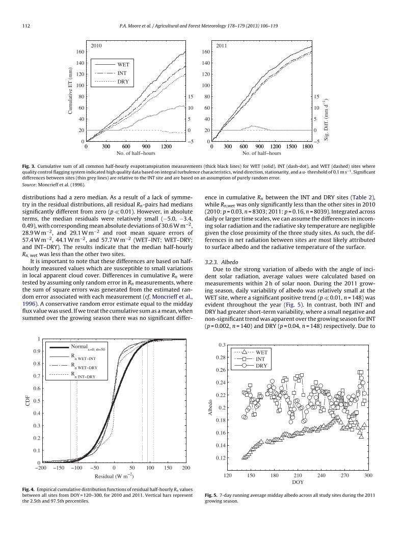
Fig. 3. Cumulative sum of all common half-hourly evapotranspiration measurements (thick black lines) for WET (solid), INT (dash-dot), and WET (dashed) sites whereq nce chd on an

S

dtst025aR

hittd1fls

Fbt

uality control flagging system indicated high quality data based on integral turbuleifferences between sites (thin grey lines) are relative to the INT site and are based

ource: Moncrieff et al. (1996).

istributions had a zero median. As a result of a lack of symme-ry in the residual distributions, all residual Rn-pairs had mediansignificantly different from zero (p � 0.01). However, in absoluteerms, the median residuals were relatively small (−5.0, −3.4,.49), with corresponding mean absolute deviations of 30.6 W m−2,8.9 W m−2, and 29.1 W m−2 and root mean square errors of7.4 W m−2, 44.1 W m−2, and 57.7 W m−2 (WET–INT; WET–DRY;nd INT–DRY). The results indicate that the median half-hourlyn, wet was less than the other two sites.

It is important to note that these differences are based on half-ourly measured values which are susceptible to small variations

n local apparent cloud cover. Differences in cumulative Rn wereested by assuming only random error in Rn measurements, wherehe sum of square errors was generated from the estimated ran-

om error associated with each measurement (cf. Moncrieff et al.,996). A conservative random error estimate equal to the middayux value was used. If we treat the cumulative sum as a mean, whenummed over the growing season there was no significant differ-

−200 −150 −100 −50 0 50 100 150 2000

0.1

0.2

0.3

0.4

0.5

0.6

0.7

0.8

0.9

1

Residual (W m−2)

CD

F

Normal

x=0; σ=50

Rn WET−INT

Rn WET−DRY

Rn INT−DRY

ig. 4. Empirical cumulative distribution functions of residual half-hourly Rn valuesetween all sites from DOY = 120–300, for 2010 and 2011. Vertical bars representhe 2.5th and 97.5th percentiles.

aracteristics, wind direction, stationarity, and a u* threshold of 0.1 m s−1. Significantassumption of purely random error.

ence in cumulative Rn between the INT and DRY sites (Table 2),while Rn,wet was only significantly less than the other sites in 2010(2010: p = 0.03, n = 8303; 2011: p = 0.16, n = 8039). Integrated acrossdaily or larger time scales, we can assume the differences in incom-ing solar radiation and the radiative sky temperature are negligiblegiven the close proximity of the three study sites. As such, the dif-ferences in net radiation between sites are most likely attributedto surface albedo and the radiative temperature of the surface.

3.2.3. AlbedoDue to the strong variation of albedo with the angle of inci-

dent solar radiation, average values were calculated based onmeasurements within 2 h of solar noon. During the 2011 grow-ing season, daily variability of albedo was relatively small at theWET site, where a significant positive trend (p � 0.01, n = 148) was

evident throughout the year (Fig. 5). In contrast, both INT andDRY had greater short-term variability, where a small negative andnon-significant trend was apparent over the growing season for INT(p = 0.002, n = 140) and DRY (p = 0.04, n = 148) respectively. Due to

120 150 180 210 240 270 300

0.12

0.14

0.16

0.18

0.2

0.22

0.24

0.26

0.28

0.3

DOY

Alb

edo

WETINTDRY

Fig. 5. 7-day running average midday albedo across all study sites during the 2011growing season.

P.A. Moore et al. / Agricultural and Forest Meteorology 178–179 (2013) 106–119 113

−100 −80 −60 −40 −20 0−120

−100

−80

−60

−40

−20

0

Lnet,DRY

(W m−2) d−1

Lne

t (W

m−

2 ) d−

1

WET v. DRYINT v. DRY

Lnet,WET

= 1.33*Lnet,DRY

− 7.4

Lnet,INT

= 1.01*Lnet,DRY

+ 0.5

Fig. 6. Correlation of daily average long-wave radiation against the DRY site for2010 and 2011 growing season data combined. The linear relation between sites isrrb

mrHi0fs

3

gsgaaLwc(sg±1abdtMbMdmtrobop

HOL HUM HOL HUM HOL HUM

−50

0

50

100

150

200

Gm

idda

y (W

m−

2 )

WET

bfi jjgg ceh dfiacdeibfacdehacdei acdeh

INT DRY

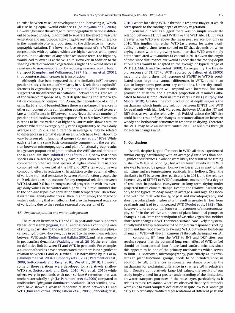
Fig. 7. Boxplots comparing daytime ground heat flux for both 2010 (black) and

epresented by the solid (WET vs. DRY) and dashed (INT vs. DRY) lines. For clarity, theelation between WET and INT has been omitted due to the close correspondenceetween INT and DRY.

id-season equipment problems with the downwelling shortwaveadiometer in 2010, full growing season albedo was not available.owever, average midday albedo at the WET site was 0.21 and 0.15

n the early and late growing season of 2010, compared to 0.13 and.17 in 2011. The change in albedo over the same period was smallor both the INT (2010: 0.23 and 0.21; 2011: 0.21 and 0.21) and DRYites (2010: 0.22 and 0.19; 2011: 0.20 and 0.21).

.2.4. Long-wave radiationAll else being equal, a simple radiation balance approach sug-

ests that a lower average albedo, such as that of the WETite, will be balanced by a higher surface temperature, and thusreater outgoing long-wave radiation. The magnitude of the dailyverage net long-wave radiation (Lnet) was comparatively hight the WET site, such that the slope of the relation betweennet,WET and Lnet,DRY (p � 0.01, slope ±SE = 1.33 ± 0.034, n = 275)as significantly greater than a 1:1 ratio (Fig. 6). The degree of

orrelation of Lnet,DRY with Lnet,WET was only somewhat lowerR2 = 0.841) than with Lnet,INT (R2 = 0.966). In addition to thetrong linear relation between Lnet,INT and Lnet,DRY over bothrowing seasons, the slope of the relation (p = 0.3034, slopeSE = 1.01 ± 0.006, n = 276) was not significantly different from:1. These results lump both day and nighttime measurements,s well as any changes throughout the season. Qualitatively, inoth study years there was no strong seasonal trend in theifference in Lnet between the INT and DRY sites, nor werehere frequent large half-hourly differences (RMSE = 7.5 W m−2,

AD = 4.2 W m−2). The magnitude of half-hourly differencesetween Lnet,WET and Lnet,DRY were greater (RMSE = 35.1 W m−2,AD = 25.5 W m−2), but the difference was largely attributable to

aytime (RMSE = 50.1 W m−2, MAD = 38.7 W m−2) versus nighttimeeasurements (RMSE = 23.3 W m−2, MAD = 18.1 W m−2). Based on

he Stefan–Boltzman law, differences in Lnet between sites areelated to the surface temperature given their close proximity to

ne another. Although the surface radiative temperature integratesoth the canopy and peat surface temperature, in the absencef canopy temperature measurements, differences in peat tem-erature measured at a depth of 0.01 m provide a qualitative

2011 (grey). Standard error estimate of the median is represented by the solid dots,and outliers by the crosses. Letters bellow each boxplot indicate where there aresignificant differences in the median.

indirect comparison. For simplicity, we focus here on the differ-ences in near-surface temperature between the WET and DRY sites.Again, the difference in half-hourly values was separated by day(Kex > 100 W m−2) and nighttime (Kex < 10 W m−2), where Kex is themodelled clear-sky incoming short-wave radiation over the grow-ing season. WET hummock temperatures were higher comparedto the DRY site with a mean daytime and nighttime difference(±STDV) of 3.0 ± 2.7 ◦C and 5.3 ± 2.3 ◦C, respectively in 2010, andsimilarly for 2011: 4.5 ± 2.1 ◦C; and 4.1 ± 3.1 ◦C. In comparison tothe mean difference in hummock temperatures, the differencein near-surface hollow temperatures between the WET and DRYsites tended to be smaller during both the day (2010: 1.9 ± 2.2 ◦C;and 2011: 0.7 ± 2.1 ◦C) and night (2010: 0.0 ± 2.0 ◦C; and 2011:0.7 ± 1.7 ◦C).

3.2.5. Ground heat fluxDifferences in peat thermal properties between sites and micro-

forms associated with � can have a strong influence on ground heatflux (G) where, for example, higher average near-surface � at theWET site should lead to higher thermal admittance and a greaterpartitioning to G. As a result of the relatively small microtopo-graphic variation and WTD, near-surface GWET,hum was consistentlygreater than GINT,hum and GDRY,hum, with values similar to Ghol. As aresult, average midday GWET was higher compared to the other sites(Fig. 7). GINT,hum and GDRY,hum were numerically similar since theywere consistently dry throughout both study years, yet they weresignificantly different as a result of near-surface �DRY,hum being con-sistently lower while having similar temperature profiles. Overall,when the proportion of hummocks and hollows was factored in, agreater proportion of Rn was partitioned to GINT than GDRY. Overall,the energy available (Ra) for turbulent fluxes is the remainder of Rn

which is not consumed by G (Table 2). The resulting cumulative day-time Ra over the growing season was 1.63 × 103 MJ, 1.83 × 103 MJ,and 1.86 × 103 MJ for the WET, INT, and DRY sites over 2010.Similarly, the corresponding values for 2011 were 1.77 × 103 MJ,1.90 × 103 MJ, and 1.92 × 103 MJ. These results indicate that in bothstudy years, there was less available energy for turbulent fluxesat the WET site. Therefore, in order to have higher ET at the WETsite, partitioning to LE must be disproportionally greater than therelative differences in Ra between sites.

3.2.6. Energy partitioningThere was a relatively large range of variability in daily energy

partitioning across all sites in both study years, where the ratio ofH to LE (ˇ) was calculated based on the sum of daytime flux values.

114 P.A. Moore et al. / Agricultural and Forest Meteorology 178–179 (2013) 106–119

120 150 180 210 240 270 300

0.5

1.0

1.5

2.0

β

WETRunning avg.

INTRunning avg.

DRYRunning avg.

120 150 180 210 240 270 300

0.5

1.0

1.5

2.0

DOY

β

WET

INT

DRY

2010

2011

F s. Linea

UdtDicI2dsostroi

3

3

u200dspgsatamrtm

ig. 8. Daily Bowen ratio for all three sites over the 2010 and 2011 growing seasonnd DRY (dashed) sites.

sing a 7-day running average, distinct trends emerge from theata (Fig. 8). In 2010, ˇ was fairly distinct at all three sites wherehe WET site tended to have the lowest average ˇ, whereas theRY site had the highest average ˇ, with the INT site taking on

ntermediate values. However, in 2011, there was a much closerorrespondence between the running average ˇ at the WET andNT sites. While, ˇ ratio values were not available during the early011 growing season at the DRY site due to instrument failure,uring the mid growing season, ˇ tended to be higher at the DRYite, with average values becoming more similar towards the endf the growing season. Independent of the differences betweenites, there was a common seasonal trend in 2010, where ˇ valuesended to decrease towards mid growing season and then remainedelatively stable. A muted version of the same early season trendccurs in 2011, where average mid to late growing season ˇ valuencreased progressively, though only by a small amount.

.3. Controls on evaporation

.3.1. ResistanceUnder near-neutral stability, the linear relation (±SE) between

*/k and uz [Eq. (5)] yielded the following estimates of z0 for010: WETz0 = 0.052 ± 0.003; INTz0 = 0.065 ± 0.027; DRYz0 =.11 ± 0.01 and 2011: WETz0 = 0.062 ± 0.009; INTz0 =.078 ± 0.013; and DRYz0 = 0.079 ± 0.06. In addition to theata on average microtopographical variation, estimates of z0uggest that the WET site was less aerodynamically rough com-ared to the other sites. All else being equal, this would implyreater aerodynamic resistance to evaporative losses at the WETite. However, when the distributions of measured wind speedre considered, the average wind speed value was ∼26% higher athe WET site compared to the other sites in both study years. Asresult of the negative correlation between wind speed and ra,

edian midday ra,WET was often significantly less than ra,INT and

a,DRY (p � 0.01) as a result of small standard error estimates, withhe exception of ra,WET and ra,INT in 2010 (p = 0.08). Nevertheless,

edian daytime values within sites and between years were

s represent the 7-day running average Bowen ratio for WET (solid), INT (dash-dot),

fairly similar (ra,WET – 55.5 s m−1, 54.2 s m−1; ram,INT – 56.5 s m−1,52.2 s m−1; and ram,DRY – 57.5 s m−1, 58.2 s m−1).

Despite the differences in ra being statistically significant, thesmall absolute difference between sites and years would have asmall effect on differences in total ET. The variability in rs betweensites, however, tended to be greater compared to ra. Overall, if weconsider median daytime rs values between sites and years, rs,WETwas 42.3 s m−1 and 44.3 s m−1, rs,INT was 55.2 s m−1 and 42.3 s m−1,and rs,DRY was 87.3 s m−1 and 74.3 s m−1 for 2010 and 2011, respec-tively. Qualitatively, rs at all sites trended downwards during the2010 growing season, while only the WET site varied seasonally in2011, with a slight increase towards the end of the growing season.Using a simple linear regression, all negative trends in 2010 weresignificantly different from zero (p � 0.01). In 2011 only rs,WET had aslope significantly different from zero (p � 0.01), whereas rs,INT andrs,DRY were not (�INT = 0.449 and �DRY = 0.02). A Jarvis-type pheno-menological model for stomatal resistance rst is typically writtenas a function of solar radiation, D, and some metric of water avail-ability. Given an appropriate scaling factor for LAI, rs is related torst and peat surface resistance. Since incoming solar radiation doesnot vary greatly between sites, the relation between rs and D wasinvestigated using equation [Eq. (6)]. Comparing the two growingseasons, the relation between rs and D only changed apprecia-bly at the WET site where bin-averaged rs values shifted higherfor most D classes in 2011 (Fig. 9). In both growing seasons, bin-averaged rs values were often highest at the DRY site, where basedon the standard error estimates, the difference was only significantbetween the WET and DRY sites in 2010. Overall, the differencebetween the WET and INT sites was less distinct, where only rs inlow D classes were significantly different in 2010. The D–rs relationonly tends to increase at low D and remains relatively constantover a range of D classes. The relative insensitivity of rs to D wouldsuggest that the sites are decoupled from atmospheric demand.The Jarvis–McNaughton decoupling coefficient (˝) can be used to

investigate the degree to which ET is linked to D through strongturbulent mixing (low ˝ values) or Ra (high ˝ values). Broadly, allthree sites have high ˝-values in both study years, where median˝WET was 0.83 and 0.79, ˝INT was 0.76 and 0.80, and ˝DRY was 0.71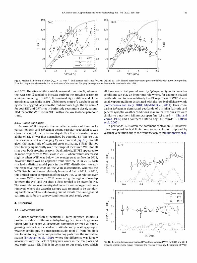

P.A. Moore et al. / Agricultural and Forest Meteorology 178–179 (2013) 106–119 115

0 0.5 1 1.5 2 2.50

30

60

90

120

150

VPD (kPa)

r s (s

m−

1 )

0 0.5 1 1.5 2 2.50

0.2

0.4

0.6

0.8

1

WET

INT

DRY

0 0.5 1 1.5 2 2.50

30

60

90

120

150

VPD (kPa)0 0.5 1 1.5 2 2.5

0

0.2

0.4

0.6

0.8

1

CD

F

20112010

F 2010E ents t

atagbfbt

3

vcatgtsbshstWttbTrip

4

4

ptgwwsal

et al., 2005).In peatlands, Rn is often the dominant control on ET; however,

there are physiological limitations to transpiration imposed byvascular vegetation due to the response of rs to D (Humphreys et al.,

0.6 0.4 0.2 0

0.2

0.4

0.6

0.8

1

ET

/PE

T &

PD

F WT

0.2

0.4

0.6

0.8

1

ET

/PE

T &

PD

F WT

WET

INT

DRY

2011

2010

ig. 9. Median half-hourly daytime (Kdwn > 100 W m−2) bulk surface resistance forrror bars represent the standard error estimate of the median. The grey line repres

nd 0.73. The sites exhibit variable seasonal trends in ˝, where athe WET site ˝ tended to increase early in the growing season tomid-summer high. In 2010, ˝ remained high until the end of therowing season, while in 2011 ˝ followed more of a parabolic trendy decreasing gradually from the mid-summer high. The trend in ˝or both INT and DRY sites in both study years more closely resem-led that of the WET site in 2011, with a shallow seasonal parabolicrend.

.3.2. Water table depthBecause WTD integrates the variable behaviour of hummocks

ersus hollows, and Sphagnum versus vascular vegetation it washosen as a simple metric to investigate the effect of moisture avail-bility on ET. ET was first normalized by potential ET (PET) so thathe seasonal effect of changing Ra was removed (Fig. 10). Overalliven the magnitude of standard error estimates, ET/PET did notend to vary significantly over the range of measured WTD for allites over both growing seasons. Qualitatively, ET/PET appeared toe more responsive to WTD class in 2010, where values decreasedlightly when WTD was below the average peat surface. In 2011,owever, there was no apparent trend with WTD. In 2010, eachite had a distinct modal peak in the WTD distribution towardshe respective high ends on the WTD distributions, whereas the

TD distributions were relatively broad and flat in 2011. In 2010,his limited direct comparison of the ET/PET vs. WTD relation overhe same WTD classes. In 2011, comparing the region of overlapetween the WET and INT sites, ET/PET tended to be lower for INT.he same relation was investigated but with wet canopy conditionsemoved, where the vascular canopy was assumed to be wet dur-ng and for several hours following rainfall events. The same generalatterns exist for dry canopy conditions in both study years.

. Discussion

.1. Evapotranspiration

A direct comparison of peatland ET rates between studies isroblematic due to differences in hydrology (e.g. fen vs. bog), vege-ation type (e.g. sedge vs. Sphagnum-dominated or treed vs. open),rowing season Rn associated with latitude, and prevailing synopticeather conditions. In a mesocosm study, total ET from fen plots

as found to be greater compared to bog plots over the snow-free

eason (Bridgham et al., 1999), where the difference was largelyssociated with the lack of Sphagnum cover in the fen plots andow early-season ET. This is in contrast to our study sites which

(a) and 2011 (b) binned based on vapour pressure deficit with 100 values per bin.he cumulative distribution of D.

all have near-total groundcover by Sphagnum. Synoptic weatherconditions can play an important role where, for example, coastalpeatlands tend to have relatively low ET regardless of WTD due tosmall vapour gradients associated with the low D of offshore winds(Sottocornola and Kiely, 2010; Liljedahl et al., 2011). Thus, com-paring Sphagnum-dominated peatlands of a similar latitude andgeneral synoptic weather conditions, maximum ET at our sites weresimilar to a northern Minnesota open fen (4.8 mm d−1 – Kim andVerma, 1996) and a southern Ontario bog (4–5 mm d−1 – Lafleur

0.6 0.4 0.2 0WTD (m)

Fig. 10. Relation between normalized ET and bin-averaged WTD for 2010 and 2011growing seasons. Grey curves represent the relative frequency distribution of WTD.

1 rest M

2AoaMtGelacd

4

atbatirotagppaioaelchswmcsttpIossnAsml(

aatnwbsrpw

16 P.A. Moore et al. / Agricultural and Fo

006) particularly as vascular LAI and canopy height increases.strong positive correlation between ET and Rn has been shown

n both a daily (Sottocornola and Kiely, 2010; Wu et al., 2010)nd seasonal (Brummer et al., 2012) timescale for peatland sites.oreover, Sonnentag et al. (2010) demonstrated that Rn explained

wice the variance in ET compared to D at a minerotrophic fen.iven our high ˝ values, the strong control of Rn on ET was alsovident at our study sites. However, because the WET site hadower Rn compared to the other two sites, and D was the samecross our sites due to their close proximity to one another, theseontrols on ET cannot explain the differences observed, particularlyuring the 2010 growing season.

.2. Albedo and surface temperature

Although Rn is similar between sites, differences in surfacelbedo which is linked to surface wetness may affect surfaceemperature, and thus may help to explain the differences in ETetween our study sites. In the absence of disturbance, surfacelbedo at a northern boreal fen has been shown to vary in responseo leaf phenology, ranging between 0.09 and 0.18 during the grow-ng season (Lafleur et al., 1997). A similar growing season trend iseported by Kellner (2001) for a Swedish bog, but with albedo beingn average 0.01 lower on wet versus dry days. Moreover, a qualita-ive relation between albedo and peat wetness was suggested fornother bog in Central Sweden where daily albedo was shown toradually increase over the growing season from 0.12 to 0.17 as theeat progressively dried (Phersson and Pattersson, 1997). Althoughlant phenology could play a role in the seasonal development oflbedo at the WET site, 2010 albedo data suggests WTD is a moremportant factor. In particular, due to the relatively low albedo ofpen water (Oke, 1987), ponding in hollows would result in a lowerlbedo at the WET site; where ponding area for our sites could bestimated from WTD and the proportion of hummocks and hol-ows. Average early and late 2010 growing season albedo valuesoincided with a WTD trend that was initially low and remainedigh during the mid and late growing season. In 2011, the growingeason trend in albedo at the WET site qualitatively correspondsith a decreasing WTD, where early season WTD was above theean peat surface. Due to the large proportion of the WET site

overed by hollows, a high WTD would coincide with significanturface ponding. This is in contrast to the INT and DRY sites werehe WTD was consistently below the mean peat surface throughouthe study period, and where hollows represent a decreasing pro-ortion of the surface. There was no trend in surface albedo at the

NT or DRY site that could be clearly linked to vascular plant phen-logy or WTD, where the higher average albedo at the INT and DRYites is consistent with a lack of ponding at these two sites. Despiteimilar covariance in albedo at the INT and DRY sites, there waso definitive correlation with surface wetness or rainfall events.lthough there was no apparent trend in albedo at the INT or DRYites associated with WTD, the relatively stable �−0.05 m for hum-ocks suggests that Sphagnum was not desiccating, thus there was

ikely no whitening response as has been observed by other studiesMcNeil and Waddington, 2003).

Although a lower albedo does not necessarily lead to greatervailable energy for turbulent fluxes, all else being equal, a lowerlbedo will result in a higher surface temperature. If we assumehat the difference in average incoming long-wave radiation isegligible between sites when integrated over a daily time step,e can infer that differences in daily net long-wave radiation can

e attributed to differences in outgoing long-wave radiation (i.e.

urface temperature). The lower average daytime net long-waveadiation at the WET site implies a higher integrated surface tem-erature. Higher near-surface (0.01 m depth) peat temperaturesere also measured in both hummocks and hollows at the WET

eteorology 178–179 (2013) 106–119

site which would help contribute to the apparent higher surfaceradiative temperature at the WET site. The degree and importanceof surface heating on energy partitioning depends on the thermalconductivity of the surface and the LAI of the vascular canopy. Fora saturated high porosity surface, such as in peatlands, a relativelylarge portion of additional energy associated with a lower albedowill be used in heating the soil profile due to the high thermaladmittance of water versus air, thus increasing potential evapo-ration due to the effect of temperature on the saturation vapourpressure. Due to the dependence of G on near-surface �, all elsebeing equal, peatlands with a greater proportion of hummocks, orconversely, peatlands with greater microtopographic variation willtend to have lower average G. At both the INT and DRY sites, theeffect of the contrast in surface wetness is apparent in the signifi-cant difference in median values (˛ = 0.05) between GINT and Ghol(Fig. 7). Kellner (2001) similarly showed higher G as a proportionof Rn in hollows versus hummocks. In comparison, the small aver-age microtopographic variation between hummocks and hollowsat the WET site lead to no significant difference in G due to similarhigh � in both microforms. When combined with a slightly lowerRn, the higher average G of the WET site leads to lower availableenergy for turbulent fluxes at the WET site.

4.3. Energy partitioning

Differences in energy partitioning between the study sitescannot be explained by higher average midday near-surface tem-perature at the WET site alone using a ‘big-leaf’ model. Assumingthe surface vapour pressure is near saturation, all else being equal,a higher surface temperature would increase ˇ in favour of thesensible heat flux. Despite low values of �−0.05 m, the assump-tion of near-saturated vapour pressure at the surface may not beunreasonable for hummocks at the INT and DRY sites. Over thecourse of the growing season, daily �INT,hum,−0.05 and �DRY,hum,−0.05did not change substantially at the daily time step in response toevaporative losses. Furthermore, the decrease in �INT,hum,−0.05 and�DRY,hum,−0.05 in 2011 with an increasing WTD was only slight. Thissuggests that either: (i) a negligible amount of water is being lostfrom the moss surface; (ii) capillary transport is able to replenishevaporative losses at a daily time step; or (iii) an extreme hydro-logical gradient exists between the moss surface and the �−0.05 mmeasurement level. Differences in energy partitioning can perhapsbe better explained by dual-source models where the lower LAIat the INT and DRY sites limit transpiration in comparison to theWET site, while increasing the relative contribution of moss sur-face evaporation. Evaporative losses from the Sphagnum surfacehave been shown to be relatively high for an LAI of 0.4–0.7 m2 m−2

(Kim and Verma, 1996), but the contribution of moss evaporationto total ET is reduced when surrounded by vascular vegetation(Heijmans et al., 2004) where our LAI values are much higher thanthose reported by Kim and Verma (1996). Moreover, despite thepotential small contribution from the moss surface given our rel-atively high LAI values, land surface schemes such as CLM includea moisture-dependent empirical term to limit surface evaporationwhich is meant to be a surrogate for molecular diffusion in theunsaturated zone (Lawrence et al., 2011). Thus, we would expectthat the greater proportion of hummocks and low near-surface �at the INT and DRY sites would serve to further limit total mossevaporation, and thus measured ET.

4.4. Aerodynamic and surface resistance

In general, our z0 values are higher than the range of valuesof 0.02–0.03 reported for a Swedish bog (Kellner, 2001), and are atthe higher end of the range reported for a Siberian bog (Shimoyamaet al., 2004). In a west Siberian bog, a qualitative relation was shown

rest M

taHevipccwsrtt

pfsotuolprpatvetitscccorWatiwo

4

bocbinar(2sWouueW

P.A. Moore et al. / Agricultural and Fo

o exist between vascular development and increasing z0 which,ll else being equal, would enhance ET (Shimoyama et al., 2004).owever, because the average microtopographic variation is differ-nt between our sites, it is difficult to separate the effect of vascularegetation and microtopography on z0. Nevertheless, the differencen the magnitude of z0 is proportional to the difference in microto-ographic variation. The lower surface roughness of the WET siteorresponds with ra values which are higher across wind speedlasses. In the absence of any other resistance term, the higher ra

ould lead to lower ET at the WET site. However, in addition to thehading effect of vascular vegetation, a higher LAI would increaseesistance to moss evaporation by reducing near-surface turbulentransport (Campbell and Williamson, 1997; Heijmans et al., 2001),hus counteracting increases in transpiration.

Although it has been suggested that the similarity in ET betweeneatland sites is the result of similarity in rs–D relations despite dif-erences in vegetation types (Humphreys et al., 2006), our resultsuggest that the difference in peatland ET between sites is the resultf the variable response of rs to D despite having the same vege-ation community composition. Again, the dependence of rs on Dsing Eq. (6) should be noted. Since there are no large differences inther component of the combination equation, rs is forced to corre-ate with difference in ET between sites. Nevertheless, a number ofeatland studies show a strong response of rs to D at low D, whereass tends to be less variable at higher D. Our results show a similarattern where the average rs only varies significantly below a dailyverage D of 0.5 kPa. The difference in average rs may be relatedo differences in stomatal resistances, which have been shown toary between plant functional groups (Korner et al., 1979). Whileach site has the same basic community composition, the correla-ion between microtopography and plant functional group resultsn a greater proportion of graminoids at the WET site and shrubs athe INT and DRY sites. Admiral and Lafleur (2007) show that shrubpecies on a raised bog generally have higher stomatal resistanceompared to other wetland species. A higher stomatal resistanceombined with lower LAI at the INT and DRY sites would have aompound effect in reducing rs. In addition to the potential effectf variable stomatal resistance between plant function groups, thes–D relation does not account for any temporal relation between

TD, LAI, and D. D has a strong seasonal progression with low aver-ge daily values in the winter and high values in mid-summer dueo the non-linear positive correlation with temperature. Therefore,f water availability influences rs, then it is not simply the degree of

ater availability that will affect rs, but also the temporal sequencef variability due to the regular seasonal progression of D.

.5. Evapotranspiration and water table position

The relation between WTD and ET in peatlands was supportedy earlier research (Ingram, 1983), and has been a continuing areaf study, in part, due to the relative complexity of modelling physi-al peat hydrology. However, due in part to the non-linear relationetween WTD and � (Kellner and Halldin, 2002), and heterogeneity

n peat surface dynamics (Waddington et al., 2010), there remainso definitive link between ET and WTD in peatlands. For example,number of studies have demonstrated that there is no significant

elation between ET and WTD when ET is normalized by PET or Rn

Shimoyama et al., 2004; Humphreys et al., 2006; Paramentier et al.,009; Sottocornola and Kiely, 2010; Wu et al., 2010). However,ome of these relations were developed for a relatively shallow

TD (i.e. Sottocornola and Kiely, 2010; Wu et al., 2010) whilethers were in peatlands with near-surface � retention that was

ncharacteristically high (i.e. Paramentier et al., 2009) compared tondisturbed Sphagnum-dominated peatlands. Other studies, how-ver, have shown a weak to moderate relation between ET andTD (Kim and Verma, 1996; Lafleur et al., 2005; Sonnentag et al.,

eteorology 178–179 (2013) 106–119 117

2010), where for a deep WTD, a threshold response may exist whichcorresponds to the rooting depth of woody vegetation.

In general, our results suggest there was no simple univariaterelation between ET/PET and WTD. For the WET site, ET/PET wasgreater when WTD was above the mean peat surface, but only in2010. This implies that either WTD (as a proxy for water avail-ability) is only a short-term control on ET that depends on whendrying occurs within a growing season, or that WTD was simplybetter correlated with another ET control in 2010. Given the lengthof time since disturbance, we would expect that the rooting depthat our sites would be adapted to the average or typical range ofWTD (cf. Mitsch and Grosselink, 2000). Consequently, the thresh-old response of ET/PET to WTD reported by Lafleur et al. (2005)may imply that a threshold response of ET/PET to WTD is pred-icated upon large inter-annual differences in WTD, rather thandue to longer term persistent dry conditions. Under dry condi-tions, vascular vegetation will respond with increased fine-rootproduction at depth, and a greater proportion of resources allo-cated to biomass production in stems versus leaves (Murphy andMoore, 2010). Greater fine root production at depth suggests themechanism which limits any relation between ET/PET and WTDfor peatlands with high LAI. Moreover, the lower LAI at the INT andDRY sites, as well as the relatively high PAI:LAI ratio at the DRY sitecould be the result of past changes in resource allocation betweenwoody and herbaceous structures in response to drying. Thereforethe WTD may have an indirect control on ET at our sites throughlong-term changes in LAI.

5. Conclusions

Overall, despite large differences in WTD, all sites experiencedsimilar energy partitioning with an average ˇ ratio less than one.Significant differences in albedo were likely the result of the timingof shallow WTD (i.e. ponding), but where lower albedo at the WETsite was balanced by greater long-wave losses due in part to highnighttime surface temperatures, particularly in hollows. Given thesimilarity in ET between sites, particularly in 2011, and the relativeinsensitivity of ET/PET to WTD fluctuations, one can infer a degreeof resilience in peatland ecosystems to long-term drying underprojected future climate change. Despite the relative insensitivityof rs to the typical midday range in average D and high ˝ associ-ated with the relatively low z0 of peatland microtopography andshort vascular plants, higher D will result in greater ET loss frompeatlands and lead to an increased WTD (Roulet et al., 1992). This,however, ignores potential long-term responses of microtopogra-phy, shifts in the relative abundance of plant functional groups, orchanges in LAI. From the standpoint of vascular vegetation, neithershort-term changes in WTD nor near-surface � are likely to system-atically limit transpiration due to the long-term response of rootingdepth and fine root growth to average WTD, but where long-termchanges in WTD will affect maximum ET through the impact on LAI.

In comparing ET from the WET to INT and DRY sites, ourresults suggest that the potential long-term effect of WTD on LAIshould be incorporated into future land surface schemes sincethis appears to be one of the primary mechanisms which servesto limit ET. Moreover, microtopography, particularly as it corre-lates to plant functional groups, needs to be included since, inaddition to LAI, differences in stomatal resistance provides themechanism for explaining difference in rs where LAI is relativelyhigh. Despite our relatively large LAI values, the results of ourstudy imply a need for a greater understanding of the limitations

on water transport processes in the moss layer, particularly as itrelates to moss resistance, where we observed that dry hummockswere able to avoid complete desiccation despite low WTD and highdaily ET. Vertically-stratified representations of different peatland

1 rest M

veesm

A

ARAweIUfstaFsa

R

A

A

A

B

B

B

B

B

C

C

C

C

C

D

D

E

18 P.A. Moore et al. / Agricultural and Fo

egetation layers in process ecosystem models (e.g., Sonnentagt al., 2008; Lawrence et al., 2011) can help to elicit whether mossvaporation is limited by vascular canopy properties or moistureupply from the underlying peat, where alternative empirical for-ulations can be used to better understand moss resistance.

cknowledgements

This research was funded by a Discovery Grant and Discoveryccelerator Supplement from the Natural Science and Engineeringesearch council of Canada to JMW and by the U.S. Department ofgriculture, grant no. 0220341 to TGP. Additional financial supportas provided by the U.S. Department of Energy’s Office of Sci-

nce (BER) through the Midwestern Regional Center of the Nationalnstitute for Climatic Change Research at Michigan Technologicalniversity. We would like to thank the U.S. Fish and Wildlife Service

or permitting access to Seney National Wildlife Refuge, and thetaff at SNWR for their kind accommodation. We also thank thewo anonymous reviewers who provided many useful commentsnd valuable suggestions which helped to improve the manuscript.inally, we would like to thank John Hribljan for his invaluableite selection, as well as Jenna Falk and Reyna Peters for their fieldssistance.

eferences

dmiral, S.W., Lafleur, P.M., Roulet, N.T., 2006. Controls on latent heat flux andenergy partitioning at a peat bog in eastern Canada. Agric. For. Meteorol. 140,308–321.

dmiral, S.W., Lafleur, P.M., 2007. Partitioning of latent heat flux at a northernpeatland. Aquat. Bot. 86, 107–116.

lbert, D.A., 1995. Regional landscape ecosystems of Michigan, Minnesota, and Wis-consin: a working classification. U.S. Department of Agriculture, St. Paul, MN,USA (Technical Report NC-178).

aldocchi, D., Valentini, R., Running, S., Oechel, W., Dahlman, R., 1996. Strategies formeasuring and modeling carbon dioxide and water vapour fluxes over terrestrialecosystems. Global Change Biol. 2, 159–168.

aldocchi, D.D., Vogel, C.A., Hall, B., 1997. Seasonal variation of energy and watervapor exchange rates above and below a boreal jack pine forest canopy. J. Geo-phys. Res. 102, 28939–28951.

aldocchi, D.D., Kelliher, F.M., Black, T.A., Jarvis, P., 2000. Climate and vegetationcontrols on boreal zone energy exchange. Global Change Biol. 6 (Suppl. 1),69–83.

ridgham, S.D., Pastor, J., Updegraff, K., Malterer, T.J., Johnson, K., Harth, C., Chen, J.,1999. Ecosystem control over temperature and energy flux in northern peat-lands. Ecol. Appl. 9 (4), 1345–1358.

rummer, C., Black, T.A., Jassal, R.S., Grant, N.J., Spittlehouse, D.L., Chen, B., Nesic, Z.,Amiro, B.D., Arain, M.A., Barr, A.G., Bourque, C.P.-A., Coursolle, C., Dunn, A., Flana-gan, L.B., Humphreys, E.R., Lafleur, P.M., Margolis, H.A., McCaughey, J.H., Wofsy,S.C., 2012. How climate and vegetation type influence evapotranspiration andwater use efficiency in Canadian forest, peatland and grassland ecosystems.Agric. For. Meteorol. 153, 14–30.

ampbell, D.I., Williamson, J.L., 1997. Evaporation from a raised peat bog. J. Hydrol.193 (1–4), 142–160.

asselman, T., 2009. Seney National Wildlife Refuge Comprehensive ConservationPlan. United States Fish and Wildlife Service, United States.

hapin, F.S., McGuire, A.D., Randerson, J., Pielke, R., Baldocchi, D., Hobbie, S.E., Roulet,N., Eugster, W., Kasischke, E., Rastetter, E.B., Zimov, S.A., Running, S.W., 2000.Arctic and boreal ecosystems of western North America as components of theclimate system. Global Change Biol. 6 (Suppl. 1), 211–223.

hivers, M.R., Turetsky, M.R., Waddington, J.M., Harden, J.W., McGuire, A.D., 2009.Effects of experimental water table and temperature manipulations on ecosys-tem CO2 fluxes in an Alaskan Rich Fen. Ecosystems 12, 1329–1342.

omer, N.T., Lafleur, P.M., Roulet, N.T., Letts, M.G., Skarupa, M., Verseghy, D.L., 1999.A test of the Canadian Land Surface Scheme (CLASS) for a variety of wetland

types. Atmos. Environ. 38, 161–179.en Hartog, G., Neumann, H.H., King, K.M., Chipanshi, A.C., 1994. Energy bud-

get measurements using eddy-correlation and Bowen-ratio techniques at theKinosheo lake tower site during the northern wetlands study. J. Geophys. Res.D. Atmos. 99, 1539–1549.

ucoudre, N.I., Laval, K., Perrier, A., 1993. SECHIBA A new set of parameterizationsof the hydrologic exchanges at the land atmosphere interface within the LMD

atmospheric general-circulation model. J. Clim. 6, 248–273.

ugster, W., Rouse, W.R., Pielke, R.A., McFadden, J.P., Baldocchi, D.D., Kittel, T.G.F.,Chapin, F.S., Liston, G.E., Vidale, P.L., Vaganov, E., Chambers, S., 2000. Land-atmosphere energy exchange in Arctic tundra and boreal forest: available dataand feedbacks to climate. Global Change Biol. 6 (Suppl. 1), 84–115.

eteorology 178–179 (2013) 106–119

Foken, T., Wichura, B., 1996. Tools for quality assessment of surface-based fluxmeasurements. Agric. For. Meteorol. 78, 83–105.

Foken, T., Gockede, M., Mauder, M., Mahrt, L., Amiro, B.D., Munger, J.W., 2004. Post-field data quality control. In: Lee, X., Massman, W.J., Law, B. (Eds.), Handbook ofMicrometeorology: A Guide for Surface Flux Measurement and Analysis. Kluwer,Dordrecht, pp. 181–208.

Frich, P., Alexander, L.V., Della-Marta, P., Gleason, B., Haylock, M., Klein Tank, A.M.G.,Peterson, T., 2002. Observed coherent changes in climatic extreme during thesecond half of the twentieth century. Climate Research 19, 193–212.

Frolking, S., Talbot, J., Jones, M.C., Treat, C.C., Kauffman, J.B., Tuittila, E.S., Roulet, N.T.,2011. Peatlands in the Earth’s 21st century climate system. Environ. Rev. 19,371–396.

Gorham, E., 1991. Northern peatlands: role in the carbon-cycle and probableresponses to climatic warming. Ecol. Appl. 1, 182–195.

Heijmans, M.M.P.D., Arp, W.J., Berendse, F., 2001. Effects of elevated CO2 and vas-cular plants on evapotranspiration in bog vegetation. Global Change Biol. 7,817–827.

Heijmans, M.M.P.D., Arp, W.J., Chapin III, F.S., 2004. Controls on moss evapora-tion in a boreal black spruce forest. Global Biogeochem. Cycles 18, GB2004,http://dx.doi.org/10.1029/2003GB002128.

Heinselman, M.L., 1965. String bogs and other patterned organic terrain near Seney,Upper Michigan. Ecology. 46 (1–2), 185–188.

Huemmrich, K.F., Kinoshita, G., Gamon, J.A., Houston, S., Kwon, H., Oechel, W.C.,2010. Tundra carbon balance under varying temperature and moisture regimes.J. Geophys. Res. 115, G000I02.

Humphreys, E.R., Lafleur, P.M., Flanagan, L.B., Hedstrom, N., Syed, K.H., Glenn,A.J., Granger, R., 2006. Summer carbon dioxide and water vapour fluxesacross a range of northern peatlands. J. Geophys. Res. 111, G04011,http://dx.doi.org/10.1029/2005JG000111.

Ingram, H.A.P., 1983. Hydrology. In: Gore, A.J.P. (Ed.), Ecosystems of the world, 4A:mires, swamp, bog, fen and moor. Elsevier Scientific Publishing Company, NewYork, pp. 67–158.

Ise, T., Dunn, A.L., Wofsy, S.C., Moorcroft, P.R., 2008. High sensitivity of peatdecomposition to climate change through water-table feedback. Nat. Geosci.1, 763–766.

Kaimal, J.C., Finnigan, J.J., 1994. Atmospheric boundary layer flows: their structureand measurement. Oxford University Press, New York, pp. 289 pp.

Kellner, E., 2001. Surface energy exchange and hydrology of a poor Sphagnum mire.Uppsala University, Sweden (Ph.D. thesis).

Kellner, E., Halldin, S., 2002. Water budget and surface-layer water storage in aSphagnum bog in central Sweden. Hydrol. Processes 16, 87–103.

Kettridge, N., Baird, A., 2006. A new approach to measuring the aerodynamic resis-tance to evaporation within a northern peatland using a modified Belanni plateatmometer. Hydrol. Processes 20, 4249–4258.

Kim, J., Verma, S.B., 1996. Surface exchange of water vapour between anopen Sphagnum fen and the atmosphere. Boundary-Layer Meteorol. 79,243–264.

Korner, C., Scheel, J.A., Bauer, H., 1979. Maximum leaf diffusive conductance invascular plants. Photosynthetica 13, 45–82.

Kowalski, K.P., Wilcox, D.A., 2003. Differences in sedge fen vegetation upstream anddownstream from a managed impoundment. Am. Midl. Nat. 150 (2), 199–220.

Lafleur, P.M., Roulet, N.T., 1992. A comparison of evaporation rates from two fensof the Hudson Bay Lowland. Aquat. Bot. 44, 59–69.

Lafleur, P.M., McCaughey, J.H., Joiner, D.W., Bartlett, P.A., Jelinski, D.E., 1997. Seasonaltrends in energy, water, and carbon dioxide fluxes at a northern boreal wetland.J. Geophys. Res. 102 (D24), 29009–29020.

Lafleur, P.M., Hember, R.A., Admiral, S.W., Roulet, N.T., 2005. Annual and seasonalvariability in evapotranspiration and water table at a shrub-covered bog insouthern Ontario. Can. Hydrol. Processes 19, 3533–3550.

Lawrence, D.M., Slater, A.G., 2008. Incorporating organic soil into a global climatemodel. Clim. Dyn. 30, 145–160, http://dx.doi.org/10.1007/s00382-007-0278-1.

Lawrence, D.M., Oleson, K.W., Flanner, M.G., Thornton, P.E., Swenson, S.C.,Lawrence, P.J., Zeng, X.B., Yang, Z.L., Levis, S., Sakaguchi, K., Bonan, G.B.,Slater, A.G., 2011. Parameterization improvements and functional and struc-tural advances in version 4 of the Community Land Model. J. Adv. Earth Syst. 3,http://dx.doi.org/10.1029/2011MS000045.

Lee, X., Massman, W.J., Law, B., 2004. Handbook of Micrometeorology: A Guide forSurface Flux Measurement and Analysis. Kluwer, Dordrecht, pp. 181–208.

Letts, M.G., Roulet, N.T., Comer, N.T., Skarupa, M.R., Verseghy, D.L., 2000.Parametrization of peatland hydraulic properties for the Canadian Land SurfaceScheme. Atmos. Ocean 38, 141–160.

Liljedahl, A.K., Hinzman, L.D., Harazono, Y., Zona, D., Tweedie, C.E., Hollister, R.D.,Endstrom, R., Oechel, W.C., 2011. Nonlinear controls on evapotranspiration inarctic coastal wetlands. Biogeosciences 8, 3375–3389.

Lund, M., Christensen, T.R., Mastepanov, M., Lindroth, A., Strom, L., 2009. Effects ofN and P fertilization on the greenhouse gas exchange in two northern peatlandswith contrasting N deposition rates. Biogeosciences 6, 2135–2144.

Massman, W.J., 2000. A simple method for estimating frequency response correc-tions for eddy covariance systems. Agric. For. Meteorol. 104, 185–198.

McNeil, P., Waddington, J.M., 2003. Moisture controls on Sphagnum growth and CO2

exchange on a cutover bog. J. Appl. Ecol. 40, 354–367.

Mitsch, W.J., Grosselink, J.G., 2000. Wetlands, third ed. John Wiley & Sons, New York,

NY.Moffat, A.M., Papale, D., Reichstein, M., Hollinger, D.Y., Richardson, A.D., Barr, A.G.,

Beckstein, C., Braswell, B.H., Chukina, G., Desai, A.R., Falge, E., Gove, J.H., Heimann,M., Hui, D., Jarvis, A.J., Kattge, J., Noormets, A., Stauch, V.J., 2007. Comprehensive

rest M

M

M

MM

M

O

OP

P

P

P

P

P

R

S

S

S

S

S

P.A. Moore et al. / Agricultural and Fo

comparison of gap-filling techniques for eddy covariance net carbon fluxes.Agric. For. Meteorol. 147, 209–232.

older, M., Kellner, E., 2001. Excess resistance of bog surfaces in central Sweden.Agric. For. Meteorol. 112, 23–30.

oncrieff, J.B., Malhi, Y., Leuning, R., 1996. The propagation of errors in long-termmeasurements of land-atmosphere fluxes of carbon and water. Global ChangeBiol. 2, 231–240.

onteith, J.L., 1973. Principles of Environmental Physics. Edward Arnold, London.onteith, J.L., 1981. Evaporation and surface temperature. Q. J. R. Meteorol. Soc.

107, 1–27.urphy, M.T., Moore, T.R., 2010. Linking root production to aboveground plant

characteristics and water table in a temperate bog. Plant and Soil 336 (1–2),219–231.

echel, W.C., Vourlitis, G.L., Hastings, S.J., Ault, R.P., Brant, P., 1998. The effects ofwater table manipulation and elevated temperature on the net CO2 flux com-ponents of Alaskan Coastal Plain tundra to shifts in water table. J. Geophys. Res.115, G00I05.

ke, T.R., 1987. Boundary Layer Climates. Routledge, New York.aavalainen, E., Paivanen, J., 1995. Peatland Forestry: Ecology and Principles.

Springer-Verlag, Berlin, pp. 248 pp.aramentier, F.J.W., van der Molen, M.K., de Jeu, R.A.M., Hendriks, D.M.D., Dol-

man, A.J., 2009. CO2 fluxes and evaporation on a peatland in the Netherlandsappear not affected by water table fluctuations. Agric. For. Meteorol. 149,1201–1208.

hersson, M., Pattersson, O., 1997. Energy and water balances of a bog in centralSweden. Nordic Hydrol. 28, 263–272.

rice, J.S., 1991. Evaporation from a blanket bog in a foggy coastal environment.Boundary-Layer Meteorol. 57 (4), 391–406.

rice, J.S., Maloney, D.A., 1994. Hydrology of a patterned bog-fen complex in south-eastern Labrador, Canada. Nordic Hydrol. 25, 313–330.

riestley, C.H.B., Taylor, R.J., 1972. On the assessment of surface heat flux and evap-oration. Mon. Weather. Rev. 106, 81–92.

oulet, N., Moore, T., Bubier, J., Lafleur, P., 1992. Northern fens: methane flux andclimatic change. Tellus: Series B 44 (2), 100–105.

himoyama, K., Hiyama, T., Fukushima, Y., Inoue, G., 2004. Controls onevapotranspiration in a west Siberian bog. J. Geophys. Res. 109, D08111,http://dx.doi.org/10.1029/2003JD004114.

onnentag, O., Chen, J.M., Roulet, N.T., Ju, W., Govind, A., 2008. Spatiallyexplicit simulation of peatland hydrology and carbon dioxide exchange:influence of mesoscale topography. J. Geophys. Res. 113, G02005,http://dx.doi.org/10.1029/2007JG000605.

onnentag, O., van der Kamp, G., Barr, A.G., Chen, J.M., 2010. On therelationship between water table depth and water vapor and carbon diox-ide fluxes in a minerotrophic fen. Global Change Biol. 16, 1762–1776,http://dx.doi.org/10.1111/j.1365-2486.2009.02032.x.

ottocornola, M., Kiely, G., 2010. Energy fluxes and evaporation mechanisms in anAtlantic blanket bog in southwestern Ireland. Water Resour. Res. 46, W11524,http://dx.doi.org/10.1029/2010WR009078.

tewart, J.B., Thom, A.S., 1973. Energy budgets in pine forest. Q. J. Roy. Meteorol.Soc. 99, 154–170.

eteorology 178–179 (2013) 106–119 119

Strack, M., Waddington, J.M., 2007. Response of peatland carbon dioxide andmethane fluxes to a water table drawdown experiment. Global Biogeochem.Cycles 21, GB1007, http://dx.doi.org/10.1029/2006GB002715.

Tanner, C.B., Thurtell, G.W., 1969. Anemoclinometer Measurements of ReynoldsStress and Heat Transport in the Atmospheric Surface Layer. ECOM 66-G22-F.University of Wisconsin, Madison, WI, USA.

Tarnocai, C., 1984. Peat Resources of Canada. Land Resource Research Institute,Research Branch, Agriculture Canada, Ottawa, Ontario, Canada.

Teklemariam, T.A., Lafleur, P.M., Moore, T.R., Roulet, N.T., Humphreys, E.R., 2010.The direct and indirect effects of inter-annual meteorological variability on

ecosystem exchange at a temperate ombrotrophic bog. Agric. For. Meteorol. 150,1402–1411.

The MathWorks, Inc., 2009. MATLAB, Version 7.8, MathWorks, Natick, Mass.Turetsky, M.R., Kane, E.S., Harden, J.W., Ottmar, R.D., Manies, K.L., Hoy, E., Kasischke,

E.S., 2011. Recent acceleration of biomass burning and carbon losses in Alaskanforests and peatlands. Nat. Geosci. 4 (1), 27–31.

Vasander, H., Kettunen, A., 2006. Carbon in boreal peatlands. In: Wider, R.K., Vitt,D.H. (Eds.), Boreal Peatland Ecosystems. Springer-Verlag, Heidelberg, Germany,pp. 165–194.

Verseghy, D.L., McFarlane, N.A., Lazare, M., 1993. CLASS – a Canadian land surfacescheme for GCMs, II, Vegetation model and coupled runs. Int. J. Climatol. 13,347–370.

Vickers, D., Mahrt, L., 1997. Quality control and flux sampling problems for towerand aircraft data. J. Atmos. Ocean. Technol. 14, 512–526.

Waddington, J.M., Kellner, E., Strack, M., Price, J.S., 2010. Differential peat defor-mation, compressibility, and water storage between peatland microforms:Implications for ecosystem function and development. Water Resour. Res. 46,W07538, http://dx.doi.org/10.1029/2009WR008802.

Walther, A., Linderholm, H.W., 2006. A comparison of growing season indices forthe Greater Baltic Area. Int. J. Biometeorol. 51, 107–118.

Webb, E.K., Pearman, G.I., Leuning, R., 1980. Correction of flux measurements fordensity effects due to heat and water vapour transfer. Q. J. Roy. Meteorol. Soc.106, 85–100.

Weltzin, J.F., Bridgham, S.D., Pastor, J., Chen, J., Harth, C., 2003. Potential effects ofwarming and drying on peatland plant community composition. Global ChangeBiol. 9, 141–151.

Whittington, P.N., Price, J.S., 2006. The effects of water table draw-down (as a sur-rogate for climate change) on the hydrology of a fen peatland, Canada. Hydrol.Process. 20, 3589–3600.

Wilcox, D.A., Sweat, M.J., Carlson, M.L., Kowalski, K.P., 2006. A water-budgetapproach to restoring a sedge fen affected by diking and ditching. J. Hydrol.320, 501–517.

Wilczak, J.M., Oncley, S.P., Stage, S.A., 2001. Sonic anemometer tilt correction algo-rithms. Boundary-Layer Meteorol. 99, 127–150.

Wu, J., Kutzbach, L., Jager, D., Wille, C., Wilmking, M., 2010. Evapotranspiration

dynamics in a boreal peatland and its impact on the water and energy balance.J. Geophys. Res. 115, G04038.

Wu, et al., 2011. Dealing with microtopography of an obrotrophic bog forsimulating ecosystem-level CO2 exchanges. Ecol. Modell. 222, 1038–1047,http://dx.doi.org/10.1016/j.ecolmodel.2010.07.015.