1

Effect of Excitation Amplitude on Disturbance Field of a

Transversely Forced Swirl Flow and Flame

Jacqueline O’Connor

Pennsylvania State University, University Park, Pennsylvania

High amplitude combustion instabilities are a destructive and increasingly pervasive problem

in gas turbine combustors. Although much research has focused on measuring the

characteristics of these instabilities, there are still many remaining questions about the fluid-

mechanic mechanisms that drive the flame oscillations. In particular, a variety of complex

disturbance mechanisms arise during velocity-coupled instabilities excited by transverse

acoustic modes. The resulting disturbance field has two components – the acoustic velocity

fluctuation from both the incident transverse acoustic field and the excited longitudinal field

near the nozzle, and the vortical velocity fluctuations arising from acoustic excitation of

hydrodynamic instabilities in the flow. In this research, we look at the relative contribution

of these two components as the amplitude of transverse excitation increases for a swirling flow

and swirl-stabilized flame in a transverse forcing combustor that mimics the geometry of an

annular combustor. Proper orthogonal decomposition is tested as a methodology for

decomposing the velocity disturbance field and is used to understand the relative contributions

of these two disturbance mechanisms.

I. Introduction

ombusiton instability in annular gas turbine engines is a pressing issue for both aircraft engines and

power generation gas turbines. Driven by the coupling between flame heat release rate fluctuation and

acoustically-excited disturbances in the combustor [1], combustion instability can lead to reduced

operability, increased emissions, and hardware damage [2]. While mitigation strategies for reducing the

impact of combustion instability are available [3, 4], better understanding of these instabilities can help

develop predictive tools for avoiding instability regimes during operation [5, 6].

This study focuses on understanding phenomena present during transverse instabilities in annular

combustor systems, particularly circumferential acoustic modes. These modes, in the 100’s of Hertz range

[7], raise additional complexity as compared to longitudinal acoustic modes, which have been the focus of

study for some time [8-14]. First, circumferential modes can be either standing-wave modes or spinning

modes, and the prediction of this condition is quite difficult as there is often no physical azimuthal boundary

condition that enforces the mode shape [15]. In either of these cases, the flame response may vary from

nozzle to nozzle, as each flame is located at a different portion of the acoustic mode across an acoustic

cycle. This makes prediction of combustion instability in a full-annular configuration difficult as the

response of each nozzle may need to be considered individually.

Next, disturbances near the flame, both pressure and velocity disturbances, can be asymmetric with respect

to the streamwise flame axis [16], as opposed to the symmetric disturbances present during longitudinal

instabilities. This asymmetry adds a layer of complexity to understanding both the disturbance field itself

[17] as well as the response of the flow field and flame [18]. Recent experimental [19] and theoretical [20]

work has shown that the net heat-release rate fluctuation across an acoustic cycle of a time-average

symmetric flame is only a function of the symmetric portion of the velocity disturbance field. This means

C

2

that purely asymmetric disturbances, within the linear regime, do not contribute to the thermoacoustic

feedback cycle for axisymmetric flames. However, flames typically are not axisymmetric in real

combustion systems, particular high-aspect-ratio geometries like annular combustors, and so the response

to asymmetric transverse excitation is a complex function of both the asymmetry of the time-average flame

shape and the velocity disturbance field. The role of both flame and disturbance field symmetry is currently

the focus of on-going work.

Finally, transverse, asymmetric forcing introduces additional possible velocity-coupling mechanisms

between the disturbance field and the flame as compared to the longitudinal mode. Previous work by this

author [21, 22] and others [23, 24] have identified several possible velocity disturbance pathways from the

original transverse acoustic field to the flame heat release rate fluctuations that drive the instability. In

general, the relevant velocity disturbances in these combustion systems can be categorized into two types:

acoustic disturbances and vortical disturbances [22, 25]. Acoustic velocity disturbances propagate at the

speed of sound and influence the flame heat release rate fluctuations both at the base of the flame – via a

base-wave mechanism [26] – and locally along the flame front. In the transversely forced system there are

two sources of acoustic velocity disturbances: the incident transverse acoustic field and the longitudinal

acoustic field that is excited by pressure fluctuations from the transverse acoustic field above the nozzle

exit. This coupling mechanism has been described by several authors in the transverse instability literature

[17, 21, 27, 28] and is the focus of much research in the rocket community, termed “injector coupling” [29].

In the current configuration, the flame is acoustically compact, meaning that the transverse acoustic

wavelength is much longer than any dimension of the flame. When the flame is located at a pressure node,

or velocity anti-node, the net acoustic velocity fluctuation through the flame is roughly zero, leading to little

net flame response from the acoustic disturbance pathway. However, when the flame is located at a pressure

anti-node, or velocity node, the transverse to longitudinal acoustic coupling can drive significant flame

response to acoustic fluctuations [28, 30].

Vortical velocity fluctuations are excited by the acoustic fluctuations and convect at a velocity on the order

of the mean flow. They can take many forms, including shear layer excitation [31], vortex breakdown

bubble excitation [11, 14], and swirl fluctuation [9, 10]. These disturbances excite local disturbances along

the flame front and can lead to significant heat release rate fluctuations. In the current configuration, the

dominant vorticity fluctuation mechanism is through shear layer rollup along the flame. Previous work in

this flow field has shown that the vortex breakdown bubble dynamics are limited as a result of the merging

of the vortex breakdown bubble with the centerbody recirculation zone, and the stagnation boundary

condition on the face of the centerbody [18]. At the acoustic velocity node, pressure anti-node forcing

condition, the shear layer response is predominantly symmetric and vortex rings are shed in both the inner

and outer shear layers; flame response stems from the vortex shedding in the inner shear layer as the flame

is stabilized there. The asymmetric forcing condition, with a pressure node and velocity anti-node, results

in helical vortex shedding in the inner and outer shear layers and asymmetric flame response.

As the amplitude of the combustor acoustics increases, the characteristics of both the velocity disturbances

and the flame heat release rate response can change. Several characterizations of flame response to high-

amplitude acoustic forcing can be found in the literature [32-34]. In particular, non-linearity in both the

flame response as well as the velocity coupling mechanisms have been measured. Limited work in the

current transverse forcing facility has shown that high amplitude excitation of the combustor can lead to

changes in the time-average structure of the flow and flame [18, 35]. For example, time-average flame

3

shape has been shown to change in the presence of high-amplitude transverse forcing, as is shown in Figure

1 from Ref. [35].

Figure 1. Line-of-sight overlays of 500 images of the flame at several forcing amplitudes a) 200 mV,

b) 400 mV, c) 600 mV, d) 800 mV, e) 1000 mV and f) 1100 mV on the function generator (transverse

acoustic fluctuation amplitudes are not available for this condition). Acoustic forcing is in-phase at

1800 Hz, flow velocity of 10 m/s, swirl number of 0.5, and equivalence ratio of 0.9 [35].

The focus of this study is to extend this work to investigate the effect of acoustic forcing amplitude on the

fluctuating characteristics of the velocity disturbance field. In particular, we wish to understand the relative

contribution of the acoustic and vortical velocity components to the overall velocity disturbance field and

what this might mean for flame response. However, it is quite difficult to separate the velocity field into

the acoustic and vortical disturbances from high-speed PIV data. Certain studies have been successful at

decomposing the acoustic and vortical disturbances using Curle’s acoustic analogy and the results agree

reasonably well with acoustic measurements [36]. These studies, however, have very well-defined velocity

boundary conditions along the perimeter of the field of view. In the current study, the field of view small

portion of the combustor interior and the boundary conditions are not well defined. Additionally, the

disparate length scales between the acoustic (on the order of meters) and vortical (on the order of

millimeters) fluctuation length scales makes separation of these disturbances difficult. Further, background

noise in the data may contaminate the acoustic velocity component calculation to the point of being

unphysical.

Previous studies of the current flow configuration have used a simplified wave superposition model to

describe the relative contributions of acoustic and vortical velocity disturbances in the transverse direction

with some success [22]. This two-wave model, however, requires curve-fitting to experimental data to

determine the amplitude of both the acoustic and vortical waves, although the convection speed of the

vortical wave and the phase between the waves was experimentally determined.

In this study, the proper orthogonal decomposition (POD) is used in an attempt to separate the acoustic

velocity fluctuations and the vortical velocity fluctuations [37]. Although these fluctuation modes will not

be automatically separated by the POD, investigation across a range of acoustic forcing conditions has

shown that for non-reacting flows, the transverse acoustic fluctuation mode can sometimes be separated

into its own eigenmode and that as the amplitude of forcing increases, this eigenmode increases in energy.

a

fed

cb

4

The results in this work show that this methodology does not work as well for reacting flows, likely as a

result of “acoustic shielding” and reflections of the acoustic field by the flame [38]. Despite this, we can

learn about the relative contribution of the acoustic and vortical velocity disturbances in the flow field from

this decomposition. Understanding the relative contribution of these disturbances can help support model

validation and further our understanding of disturbance mechanisms during thermoacoustic instability.

The remainder of this paper is organized as follows. First, an overview of the experimental facility provides

details about the combustor, the acoustic forcing configuration, the diagnostics, and the test matrix. Next,

the data analysis methods are briefly explained. Results for both the time-average and time-varying

components of the flow field are provided for both non-reacting and reacting flow. Finally, we draw

conclusions about this work and its application towards better understanding and controlling combustion

instabilities in gas turbines.

II. Experimental overview

A single-nozzle combustor with transverse-forcing capability was used in this series of tests, as shown in

Figure 2. This high-aspect-ratio combustor configuration is used to mimic both the dimensions and acoustic

mode of an annular combustion chamber. The inner dimensions of the combustion chamber are 114.3 cm

x 35.56 cm x 7.62 cm, with the long dimension in the transverse direction. The nozzle is located at the

center of the long dimension and the five 5.08 cm exhaust ports are located 35.56 cm downstream. The

center exhaust port, located directly downstream of the nozzle, is covered with optical-grade quartz glass

in these tests to protect the laser optics downstream. The nozzle has an outer diameter of 3.18 cm and a

centerbody with a diameter of 2.18 cm. The 12-bladed, non-aerodynamic swirler is located 5.08 cm

upstream of the dump plane and has a geometric swirl number of 0.85 [39]. Upstream of the swirler is a

large settling chamber that is used to both reduce incoming turbulence and acoustically isolate the

combustor from the air and fuel lines. A perforated plate is located inside the chamber to break up large-

scale turbulent structures from the air/fuel feed line.

Figure 2. Experimental setup with combustor, acoustic drivers, and settling chamber. Diagnostics

not shown.

In both non-reacting and reacting experiments, air is supplied with a bulk velocity of 10 m/s at the nozzle

exit. In the reacting experiments, natural gas is mixed with the air well upstream of the settling chamber

5

and can be assumed to be fully premixed; the equivalence ratio is 0.9. The exhaust is far downstream of

the exit ports of the combustor, as can be seen in Figure 2.

Acoustic forcing

Acoustic forcing is provided by two sets of three speakers, one set on either end of the combustor. The

speakers are located at the end of extendable tubes, tuned to 100 cm in these experiments. The speaker

tubes attach to the combustor at the end of the long dimension to avoid acoustic streaming in the region of

the nozzle. These two banks of speakers are operated so as to create a standing-wave pattern in the

combustor; both preliminary experimental work and extensive acoustic modeling using Comsol

Multiphysics [17] have indicated that the transverse acoustic mode is planar in the region of the nozzle over

a frequency range of approximately 400-1200 Hz.

Two modes of the standing wave have been investigated in this study. First, when the two banks of speakers

are operated in-phase, this creates a pressure anti-node at the nozzle and will be referred to as “in-phase

forcing.” Next, when the two banks of speakers are operated at a phase of 180°, a pressure node is created

at the nozzle; this will be referred to as “out-of-phase forcing.” Spatial averages of the transverse flow

velocities were calculated in order to determine representative values of the amplitude of acoustic forcing

at each condition. The reference transverse velocity fluctuation, see Equation 1, was obtained from an

average of local values over one outer jet diameter downstream along the centerline of the flow. The Fourier

transform of the integrated velocity was then calculated and the amplitude at the forcing frequency

extracted.

21

( ) ( , 0, ) D

T

D

u t v x r t dxD

(1)

Figure 3. Amplitude of the reference normalized transverse velocity fluctuations at the

forcing frequency as a function of speaker input voltage, at uo=10 m/s, S=0.85.

6

Figure 3 plots the measured spatially-averaged transverse reference velocity fluctuation, uT, at the

forcing frequency for the range of conditions presented in this work. It shows that the transverse disturbance

amplitude at the forcing frequency rises almost linearly with excitation voltage. As expected, the out-of-

phase cases shown in Figure 3 have higher transverse velocity amplitudes than their in-phase counterparts

at the same frequency. The in-phase forcing cases have non-zero transverse amplitudes as a result of

imbalances in the forcing system. For example, speakers on the left and right may not be operating at

exactly the same amplitude and so the velocity node is not located directly along the nozzle centerline.

Diagnostics

Velocity measurements in this study were made using high-speed particle image velocimetry (PIV). The

laser is a Litron Lasers Ltd. LDY303He Nd:YLF laser with a wavelength of 527 nm and a 5 mJ/pulse pulse

energy at the 10 kHz repetition rate used for these experiments. The Photron HighSpeed Star 1.1 camera

has a 640x448 pixel resolution with 20x20 micron pixels on the sensor at a frame rate of 10 kHz. A

LaVision divergent sheet optic, with an f = -20 mm cylindrical lens, was used to create a 1 mm thick sheet.

The sheet entered the experiment from a window at the exit plane of the combustor and reached a width of

approximately 12 cm at the dump plane. This alignment is referred to as the x r alignment. Aluminum

oxide seed particles with a mean diameter of 2 microns were used. Image pairs were taken with a separation

time, dt, of nominally 20 microseconds for the x r alignment.

Velocity field calculations were performed using DaVis 7.2 software from LaVision. The velocity

calculation was done using a three-pass operation: the first pass at an interrogation window size of 64x64

pixels, the second two passes at an interrogation window size of 32x32, each with an overlap of 50%. Each

successive calculation uses the previously calculated velocity field to better refine the velocity vector

calculation; standard image shifting techniques are employed in the calculation. The correlation peak is

found with two, three-point Gaussian fits and average values of the correlation peak ranged from 0.4 to 1

throughout the velocity field. There were three vector rejection criteria used both in the multi-pass

processing steps and the final post-processing step. First, velocity vectors with magnitudes greater than 25

m/s were rejected as unphysical for this specific flow. Second, median filtering was used to filter points

where surrounding velocity vectors had an RMS value greater than three times the local point. This filter

is used to rid the field of spurious vectors that occur due to issues with imaging, particularly near boundaries.

Third, groups of vectors greater than five vectors were removed; this operation removes errors caused by

local issues with the original image, including window spotting, and are aggravated by using overlapping

interrogation windows. Finally, vector interpolation was used to fill the small spaces of rejected vectors.

Overall, an average of 8% of vectors are rejected and replaced with interpolated values.

Test Matrix

Several tests were performed to understand the effect of amplitude on the velocity disturbance field in the

transversely forced swirling flow. Table 1 provides a list of data that are discussed in this study. Most of

the data referred to in this study was taken at non-reacting conditions, although two reacting cases are

shown as a basis of comparison.

7

Table 1. Test matrix for velocity measurements.

Frequency [Hz] Forcing Amplitude range [m/s] Reacting/Non

400 Out-of-phase 1, 2, 4.2, 6 non-reacting

400 In-phase 0.2, 0.5, 0.7 non-reacting

400 Out-of-phase 4.2, 6 reacting

Data Analysis

The main data analysis method used in this study was POD of the velocity field into spatial and temporal

eigenmodes [37]. This is a common decomposition method for fluctuating flow fields that helps to illustrate

the major contributions to the fluctuating disturbance field. The results of this analysis produce a spatial

mode shape and a temporal mode amplitude; here the fast Fourier transform (FFT) of the temporal mode

amplitude is presented in order to analyze the spectral content of each mode’s oscillation.

In this analysis, 500 instantaneous, two-dimensional velocity fields from PIV were used to calculate the

modes, where the data were obtained at 10 kHz. The time-average field was subtracted from the data before

the POD analysis so as to only decompose the fluctuating component. The spatial modes presented here

are the normalized modes, and the temporal component has been calculated from those normalized modes.

As a result, we do not try to extract a physical unit from the amplitude of the temporal component, but

amplitudes can be compared across different sets of data. The temporal amplitudes are presented using the

fast Fourier transform, where the frequency resolution is 20 Hz.

III. Results

Time-average flow field

The time-average flow field is typical of a highly swirling flow field; an annular jet surrounds a large vortex

breakdown region along the centerline. The r-x view of the flow field is provided in Figure 4 for both non-

reacting (left) and reacting (right) flows. In the axial velocity field, the annular jet is shown originating from

the annular gap and it passes around the centrally located wake/vortex breakdown region. The shear layers

shown in the time-average vorticity plot arise from the mixing of the annular jet and the inner recirculation

zone, forming the inner shear layer, and the quiescent flow around the jet, forming the outer shear layer.

The inner shear layer is stronger than the outer, presumably because the velocity gradient between the jet

and the recirculating flow in the vortex breakdown region is greater than that between the jet and the

quiescent fluid outside the jet.

The time-averaged flow fields of the non-reacting and reacting cases differ in several ways. First, the vortex

breakdown bubble changes in size and shape, and is generally wider in the reacting case. Second, the jet

spreading angle is higher in the reacting case, presumably because of the wider vortex breakdown bubble.

Third, the average shear layer locations, as shown by the vorticity plots, also spread as a result of the two

aforementioned effects. The time-average jet velocity is higher in the reacting case, a result of expansion

from the flame; as a result, the time-average shear layer strengths are also greater than in the reacting data.

Note that this flow contains two distinct shear layers, one emanating from the inner edge and one from the

outer edge of the annulus. The flame configuration is nominally that of a “V-shape” stabilized in the inner

shear layer only. Examples of the time-average flame shape are in Figure 1.

8

a) b)

Figure 4. Time-averaged a) axial velocity and b) vorticity fields at Uo=10 m/s, swirl number of 0.85,

non-reacting flow (left) and reacting flow (right), equivalence ratio of 0.9 with natural gas fuel.

Axial velocity is normalized by the bulk velocity, Uo, and vorticity is normalized by the bulk velocity

divided by the annular gap width, Uo/(r2-r1).

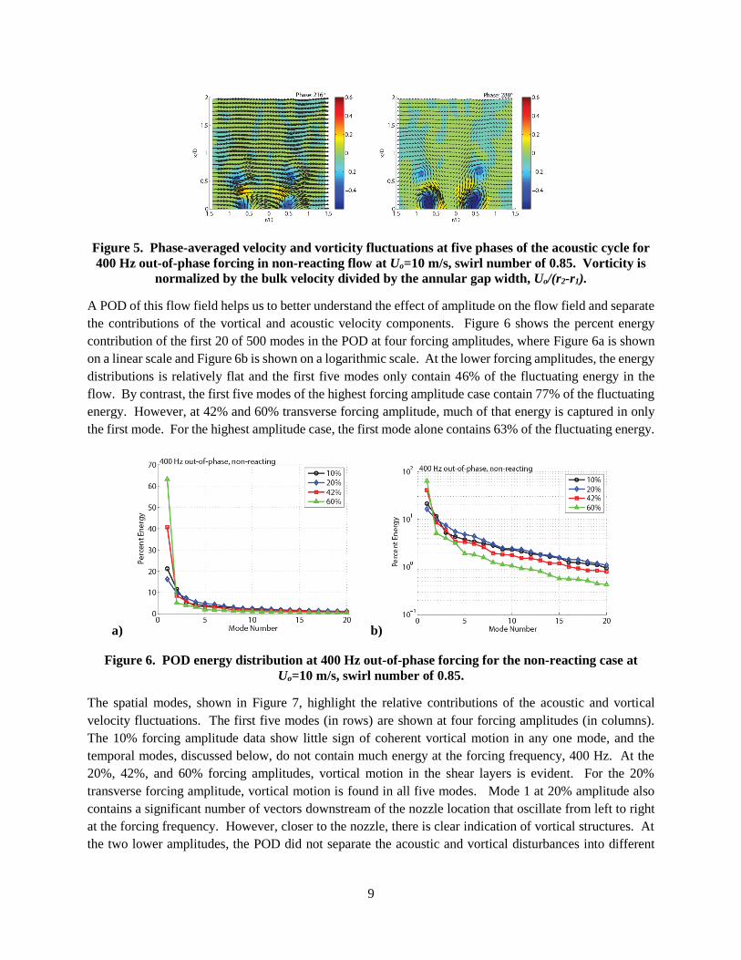
Effect of amplitude at 400 Hz out-of-phase – non-reacting

In the out-of-phase cases, the nozzle is located at an acoustic velocity anti-node and a pressure node,

resulting in an asymmetric velocity disturbance field. This asymmetry in the acoustic field excites an

asymmetric response in the shear layers, as is indicated in the phase-averaged vorticity fluctuation plots in

Figure 5. These data, taken from the uT=4.2 m/s case for clarity, show an asymmetric pattern in the vorticity

fluctuation, as the shear layer sheds in a helix. In a plane of the flow, this vortex rollup looks like alternate

vortices shedding from the dump plane on either side of the nozzle centerline. The asymmetry of the flow

field is visible in the vorticity contours on either side of the centerline, keeping in mind the 180 offset in

vorticity fluctuation magnitude that arises from the differences in sign of vorticity on either side of the

centerline. In the flow field far from the nozzle, where the vortical velocity fluctuations have dissipated,

the velocity fluctuations predominantly stem from the transverse acoustic field. This is quite evident from

the velocity vectors in Figure 5, where the vectors oscillate from pointing almost entirely left (at 0 degrees

phase) to entirely right (near 144 degrees phase). Closer to the dump plane, however, the velocity

fluctuations are a combination of acoustic and vortical velocity.

9

Figure 5. Phase-averaged velocity and vorticity fluctuations at five phases of the acoustic cycle for

400 Hz out-of-phase forcing in non-reacting flow at Uo=10 m/s, swirl number of 0.85. Vorticity is

normalized by the bulk velocity divided by the annular gap width, Uo/(r2-r1).

A POD of this flow field helps us to better understand the effect of amplitude on the flow field and separate

the contributions of the vortical and acoustic velocity components. Figure 6 shows the percent energy

contribution of the first 20 of 500 modes in the POD at four forcing amplitudes, where Figure 6a is shown

on a linear scale and Figure 6b is shown on a logarithmic scale. At the lower forcing amplitudes, the energy

distributions is relatively flat and the first five modes only contain 46% of the fluctuating energy in the

flow. By contrast, the first five modes of the highest forcing amplitude case contain 77% of the fluctuating

energy. However, at 42% and 60% transverse forcing amplitude, much of that energy is captured in only

the first mode. For the highest amplitude case, the first mode alone contains 63% of the fluctuating energy.

a) b)

Figure 6. POD energy distribution at 400 Hz out-of-phase forcing for the non-reacting case at

Uo=10 m/s, swirl number of 0.85.

The spatial modes, shown in Figure 7, highlight the relative contributions of the acoustic and vortical

velocity fluctuations. The first five modes (in rows) are shown at four forcing amplitudes (in columns).

The 10% forcing amplitude data show little sign of coherent vortical motion in any one mode, and the

temporal modes, discussed below, do not contain much energy at the forcing frequency, 400 Hz. At the

20%, 42%, and 60% forcing amplitudes, vortical motion in the shear layers is evident. For the 20%

transverse forcing amplitude, vortical motion is found in all five modes. Mode 1 at 20% amplitude also

contains a significant number of vectors downstream of the nozzle location that oscillate from left to right

at the forcing frequency. However, closer to the nozzle, there is clear indication of vortical structures. At

the two lower amplitudes, the POD did not separate the acoustic and vortical disturbances into different

10

modes, and as a result, this method would not work for quantifying the relative contribution of these

disturbances to the overall disturbance field.

Figure 7. First five spatial POD modes (rows) for 400 Hz out-of-phase forcing at Uo=10 m/s, swirl

number of 0.85 in non-reacting flow at four forcing amplitudes (columns).

At the two higher amplitudes, however, the POD seems to separate the contributions from the acoustic

motions, which are shown in Mode 1, and vortical contributions in Modes 2-5. In Mode 1 of both cases,

the majority of vectors are all pointing in one transverse direction, signaling that these oscillations stem

from the transverse acoustic field as no vortical disturbances in the flow field are that uniformly

unidirectional. When reconstructed with its temporal amplitude, Mode 1 also shows transverse oscillatory

behavior in the far field. Closer to the nozzle, the velocity fluctuations in Mode 1 at both 42% and 60%

forcing amplitude point in (on the left) and out (on the right) of the nozzle’s annular passage. This

longitudinal oscillation is an indication of the transverse to longitudinal acoustic coupling at the nozzle exit

11

that has been described in previous work [21]. Vortical velocity fluctuations at the two highest amplitudes

are found in Modes 2 and higher, although there may be some acoustic energy in those modes as well. The

vortical disturbances are mostly located in the shear layer, which corresponds to the vortical fluctuations

that were present in the phase-averaged images in Figure 5.

The spectra of the first five temporal modes at four forcing amplitudes are in Figure 8, where the spectra

for Mode 1 are shown on both a linear and logarithmic scale for clarity. Most of the spectra have a peak at

400 Hz, the forcing frequency at this condition. Both acoustic and vortical velocity fluctuations can

contribute to this peak because the shear layer instability responds to the acoustics at the forcing frequency.

Additionally, each of the modes has some low-frequency content between 0 and 160 Hz. Similar low-

frequency content was measured, particularly at low forcing amplitudes, in previous studies of the vortex

breakdown bubble in this flow field [18]. These motions are likely due to motion within the vortex

breakdown bubble and will not be considered in detail here as they do not play a significant role in the

flame response to the transverse acoustic field.

12

Figure 8. FFTs of the first five temporal POD modes for 400 Hz out-of-phase forcing at Uo=10 m/s,

swirl number of 0.85 in non-reacting flow. Mode 1 is shown on both a linear (left, top) and

logarithmic (right, top) scale.

The Mode 1 spectra show relatively strong 400 Hz oscillations at all four forcing amplitudes, although the

oscillations at the 10% forcing amplitude are quite small compared to those of the other three forcing

amplitudes. As the forcing amplitude increases, the strength of the 400 Hz peak increases and the low-

frequency content is suppressed. This is further evidence that at the two higher forcing amplitudes the

velocity fluctuations are predominantly acoustic. The low frequency motion remains in the spectra of the

other modes, even at the high forcing amplitudes, but is removed from Mode 1.

Another feature of the high amplitude spectra is the presence of several harmonics at 800 Hz, 1200 Hz, and

1600 Hz. These harmonics could arise from two sources; they could be the result of non-linearity in the

incident acoustic field or non-linear response in the flow field. The harmonics most likely stem from non-

linearity in the incident forcing signal for two reasons. First, the dominant velocity fluctuation in Mode 1

for 42% and 60% forcing is acoustic, not vortical, and so any non-linearities in the shear layer response

would not register. Further, pressure measurements taken inside the nozzle (see Ref. [19] for details of

these measurements) show pressure spectra with a similar shape.

Figure 9. Comparison of the FFTs of the Mode 1 temporal POD mode and the pressure fluctuation

at the same forcing amplitude for 400 Hz out-of-phase forcing at 60% amplitude, Uo=10 m/s, swirl

number of 0.85 in non-reacting flow.

13

Figure 9 shows a comparison of the FFT of the Mode 1 temporal mode at the highest forcing amplitude,

60% of the mean flow velocity, and the pressure amplitude measured at the same condition. Both spectra

have been normalized by the amplitude at the forcing frequency, 400 Hz, so as to compare the relative

strengths of the harmonic signatures between the two signals. It is quite evident that the ratio between the

harmonic strength and the fundamental is almost the same for both the pressure and Mode 1 velocity

fluctuations, indicating that the non-linearity is likely stemming from the input acoustics.

Focusing now on the Modes 2-5 spectra for the three highest forcing amplitudes, it is evident that the

relationship between the 400 Hz signal strength and forcing amplitude is no longer monotonic. For

example, the highest 400 Hz peak for Mode 2 is from the 60% amplitude case, followed by the 20% then

the 42% cases in order of reducing strength. The relative strength of the low-frequency content also varies

in similar ways for Mode 2. Non-monotonic variation in 400 Hz and low-frequency peak strengths is seen

in Modes 3 and 5, and in Mode 4, there is very little 400 Hz content and the low-frequency motion

dominates. It is difficult to correlate the frequency content with any particular portion of the spatial modes

as the overall vortical motion is divided between so many modes, including those higher than Mode 5.

Another feature of these spectra is the absence of significant higher harmonics or any other non-linearity

signatures, such as sum-and-difference frequencies. This indicates that the shear layer response is still

linear, even at these high amplitudes of acoustic forcing. Any non-linearity in the flame response would

stem not from non-linearity in the flow response, but instead non-linearity in the flame dynamics. This is

in contrast to the results from similar flow fields, such as those from Thumuluru and Lieuwen [11]; in that

study, however, the non-linearity in the flow field stemmed from the vortex breakdown bubble, the result

of an absolute instability whose response to acoustics is negligible in the linear regime. As the vortex

breakdown bubble does not play an important dynamical role in this flow field or the response of this flame,

non-linearity in the flow field is not detected as the amplitude increases.

Figure 10. Comparison of Mode 1 (mostly acoustic) and Modes 2-5 (most vortical) spectra at 42%

(left) and 60% (right) forcing amplitudes for 400 Hz out-of-phase forcing, Uo=10 m/s, swirl number

of 0.85 in non-reacting flow.

This analysis shows that at high forcing amplitudes, a POD can help to separate the relative contribution of

acoustic and vortical velocity fluctuations to the overall fluctuating flow field. To compare the strength of

these motions at the two highest forcing amplitudes, the spectra of Mode 1 is compared with the spectra of

Modes 2-500, where the mode energies were superimposed before the Fourier transform was performed.

14

These comparisons are in Figure 10. The comparisons of the spectra for Mode 1 and Modes 2-5 not only

show the relative contribution of the approximate acoustic and vortical components of the velocity

fluctuation, but also the frequency content of each signal. At 42% amplitude, the vortical fluctuations are

greater than the acoustic at 400 Hz, and there is broadband frequency content that stems from both coherent

motion, particularly in the low-frequency range, and turbulence. At 60% forcing condition, the acoustic

and vortical velocity fluctuation amplitudes are almost equal at 400 Hz. These high-amplitude results

mirror the curve-fit results discussed in Ref. [22].

Effect of amplitude at 400 Hz in-phase – non-reacting

The second condition is the in-phase forcing case, where a pressure anti-node along the centerline creates

a symmetric acoustic forcing condition and excites longitudinal fluctuations at the nozzle exit. The

measured transverse amplitude of these modes is low, as described in the Experimental Overview section,

although the speaker voltage amplitude is high. Figure 11 shows the phase-averaged velocity and vorticity

fluctuation fields at several phases of the acoustic cycle for the highest in-phase forcing amplitude; the

structure of the phase-averaged fluctuating flow field is similar at all forcing amplitudes and the highest

amplitude is shown for clarity.

Figure 11. Phase-averaged velocity and vorticity fluctuations at five phases of the acoustic cycle for

400 Hz in-phase forcing in non-reacting flow at Uo=10 m/s, swirl number of 0.85. Vorticity is

normalized by the bulk velocity divided by the annular gap width, Uo/(r2-r1).

At this forcing condition, the axisymmetric acoustic disturbance field excites symmetric shear layer

shedding, which manifests as vortex rings that separate at the dump plane and convect downstream. The

vorticity fluctuation in Figure 11 is symmetric on either side of the centerline and the coherent structures

from the vortex shedding are clearly visible. The velocity fluctuation in the far field, away from the nozzle,

is small in magnitude and the direction is mostly transverse. This velocity fluctuation is predominantly

from the acoustics as the vortical structures have dissipated since then, as evidenced by the near zero

vorticity fluctuation levels. The imbalance in the acoustic field that leads to a non-zero acoustic velocity

15

fluctuation along the centerline is evident in these data. At 72 degrees phase, the velocity fluctuation node

seems to be quite close to the centerline of the nozzle, where it would be located in a perfectly balanced

system. However, the node moves in location; at 0 and 216 degrees, it seems to be to the left of the nozzle,

and at 144 and 200 degrees, it seems to be to the right. Despite this imbalance in the acoustic velocity, the

wavelength of the 400 Hz wave is long such that the pressure anti-node at this location is large enough in

magnitude to drive an axisymmetric pulsing in the nozzle and symmetric vortex rollup in the shear layers.

Figure 12. Energy distribution for 400 Hz in-phase forcing for the non-reacting case at Uo=10 m/s,

swirl number of 0.85.

A POD of this fluctuating flow field at four forcing amplitudes reveals more information about the

fluctuating component of the velocity field. Unlike the out-of-phase forcing cases where a significant

portion of the velocity fluctuation comes from the acoustic component at the velocity anti-node, the energy

distribution for the in-phase forcing cases is more gradual. Also unlike the out-of-phase forcing cases, the

distributions in the in-phase forcing cases become more gradual with higher forcing amplitude without the

large peak in the Mode 1 energy that was present in Figure 6.

The spatial mode distributions for the in-phase forcing cases present a more ambiguous decomposition of

the velocity disturbance field than they did in the out-of-phase forcing case. As noted above, the lack of

significant acoustic velocity fluctuations reduces the overall velocity fluctuation energy in the higher

modes, shown here. Little evidence of transverse velocity fluctuation stands out in any one mode, as in the

out-of-phase forcing case, although vortical velocity fluctuations are evident in several of the modes at all

forcing amplitudes.

16

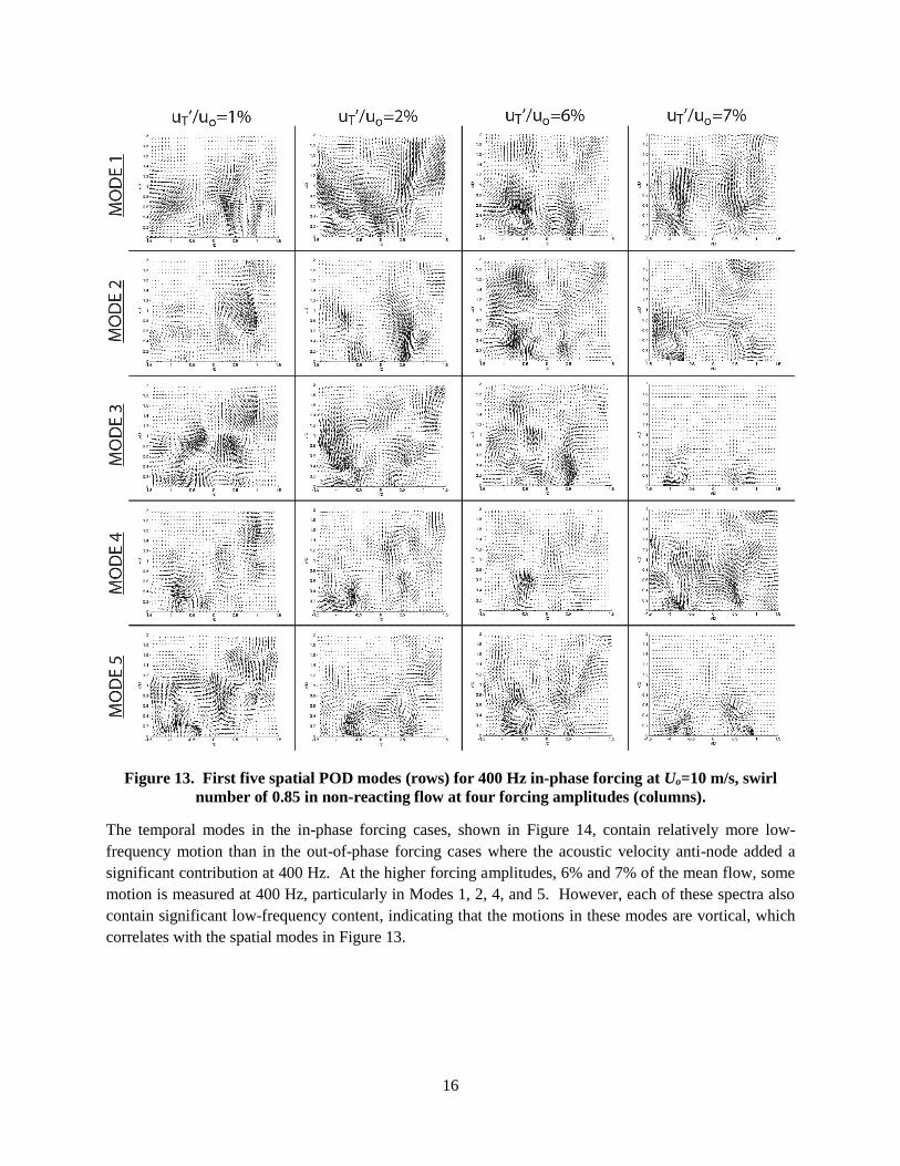
Figure 13. First five spatial POD modes (rows) for 400 Hz in-phase forcing at Uo=10 m/s, swirl

number of 0.85 in non-reacting flow at four forcing amplitudes (columns).

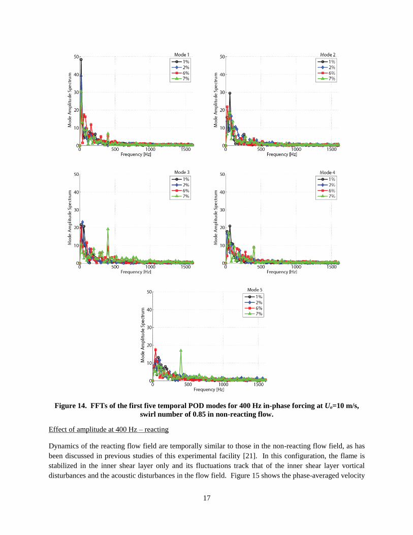
The temporal modes in the in-phase forcing cases, shown in Figure 14, contain relatively more low-

frequency motion than in the out-of-phase forcing cases where the acoustic velocity anti-node added a

significant contribution at 400 Hz. At the higher forcing amplitudes, 6% and 7% of the mean flow, some

motion is measured at 400 Hz, particularly in Modes 1, 2, 4, and 5. However, each of these spectra also

contain significant low-frequency content, indicating that the motions in these modes are vortical, which

correlates with the spatial modes in Figure 13.

17

Figure 14. FFTs of the first five temporal POD modes for 400 Hz in-phase forcing at Uo=10 m/s,

swirl number of 0.85 in non-reacting flow.

Effect of amplitude at 400 Hz – reacting

Dynamics of the reacting flow field are temporally similar to those in the non-reacting flow field, as has

been discussed in previous studies of this experimental facility [21]. In this configuration, the flame is

stabilized in the inner shear layer only and its fluctuations track that of the inner shear layer vortical

disturbances and the acoustic disturbances in the flow field. Figure 15 shows the phase-averaged velocity

18

and vorticity fluctuations for the 400 Hz out-of-phase forcing case in reacting flow. Like the non-reacting

case, vortical fluctuations are visible in the shear layers, and transverse motion is visible in the far field,

particularly at 144 and 288 degrees phase. The vortical fluctuations are stronger and persist farther

downstream in the reacting case than in the non-reacting case, a probable result of the higher mean-shear

in the shear layers that was shown in Figure 4. As a result of the stronger vortical fluctuations far from the

nozzle, the shape of the transverse acoustic forcing field is not as evident as in the non-reacting case in the

phase-averaged images. The asymmetry of the flow field, a result of asymmetric acoustic forcing, is visible

in the vorticity contours on either side of the centerline, keeping in mind the 180 offset in vorticity

fluctuation magnitude that arises from the differences in sign of vorticity on either side of the centerline.

Figure 15. Phase-averaged velocity and vorticity fluctuations at five phases of the acoustic cycle for

400 Hz out-of-phase forcing in reacting flow at uT/Uo=42%, Uo=10 m/s, swirl number of 0.85.

Vorticity is normalized by the bulk velocity divided by the annular gap width, Uo/(r2-r1).

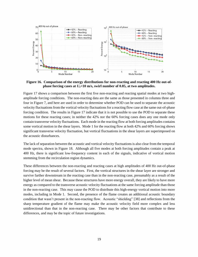
A POD of the reacting flow field at two forcing amplitudes shows the dominant motions in the flow field.

Figure 16 shows a comparison between the energy distribution of the POD in the reacting flow at two

forcing amplitudes and the companion non-reacting cases, both at 42% and 60% transverse forcing. The

plot on the left shows the energy distribution of the first 20 modes on a linear scale, and the plot on the right

shows the energy distribution of the first 20 modes on a logarithmic scale for better visualization of the

decay of mode energy with increasing mode number. The most noticeable difference between the non-

reacting and reacting cases is the contribution of Mode 1 at these two high-amplitude forcing conditions.

In the non-reacting cases, Mode 1 contributes 41% and 63% of the total energy in the 42% and 60% forcing

cases, respectively. For the reacting conditions, however, the Mode 1 energies are much lower: 7% at 42%

forcing amplitude and 15% at 60% forcing. The energy distributions for the reacting cases are also flatter

than those in the non-reacting cases, which is clearer to see on the logarithmic scale than on the linear.

19

Figure 16. Comparison of the energy distributions for non-reacting and reacting 400 Hz out-of-

phase forcing cases at Uo=10 m/s, swirl number of 0.85, at two amplitudes.

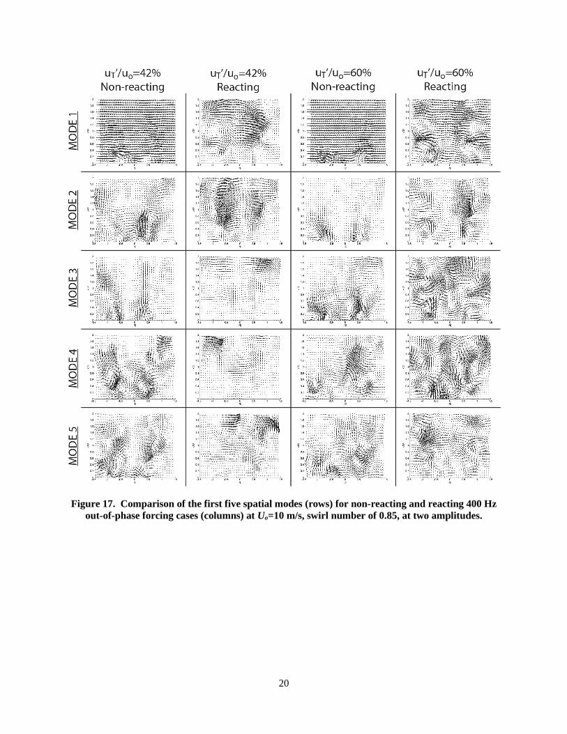
Figure 17 shows a comparison between the first five non-reacting and reacting spatial modes at two high-

amplitude forcing conditions. The non-reacting data are the same as those presented in columns three and

four in Figure 7, and here are used in order to determine whether POD can be used to separate the acoustic

velocity fluctuations from the vortical velocity fluctuations for a reacting flow case at the same out-of-phase

forcing condition. The results in Figure 17 indicate that it is not possible to use the POD to separate these

motions for these reacting cases; in neither the 42% nor the 60% forcing cases does any one mode only

contain transverse velocity fluctuations. Each mode in the reacting flow at both forcing amplitudes contains

some vortical motion in the shear layers. Mode 1 for the reacting flow at both 42% and 60% forcing shows

significant transverse velocity fluctuation, but vortical fluctuations in the shear layers are superimposed on

the acoustic disturbances.

The lack of separation between the acoustic and vortical velocity fluctuations is also clear from the temporal

mode spectra, shown in Figure 18. Although all five modes at both forcing amplitudes contain a peak at

400 Hz, there is significant low-frequency content in each of the signals, indicative of vortical motion

stemming from the recirculation region dynamics.

These differences between the non-reacting and reacting cases at high amplitudes of 400 Hz out-of-phase

forcing may be the result of several factors. First, the vortical structures in the shear layer are stronger and

survive farther downstream in the reacting case than in the non-reacting case, presumably as a result of the

higher level of mean shear. Because these structures have more energy overall, they are likely to have more

energy as compared to the transverse acoustic velocity fluctuations at the same forcing amplitude than those

in the non-reacting case. This may cause the POD to distribute this high-energy vortical motion into more

modes, including in Mode 1. Second, the presence of the flame creates an additional acoustic boundary

condition that wasn’t present in the non-reacting flow. Acoustic “shielding” [38] and reflections from the

sharp temperature gradient of the flame may make the acoustic velocity field more complex and less

unidirectional than that in the non-reacting case. There may be other factors that contribute to these

differences, and may be the topic of future investigations.

20

Figure 17. Comparison of the first five spatial modes (rows) for non-reacting and reacting 400 Hz

out-of-phase forcing cases (columns) at Uo=10 m/s, swirl number of 0.85, at two amplitudes.

21

Figure 18. Spectra of the first five temporal modes for reacting 400 Hz out-of-phase forcing cases

at Uo=10 m/s, swirl number of 0.85, at two amplitudes.

IV. Conclusions

This study investigates the effect of transverse acoustic excitation amplitude on both a non-reacting and

reacting swirling flow by using proper orthogonal decomposition. In particular, this decomposition is used

to understand the relative contributions of vortical and acoustic velocity fluctuations in the flow field that

could lead to flame response. Understanding the relative role of these contributions could be an important

22

step towards more accurate reduced-order modeling and validation of higher-order models with this type

of high-speed, high-fidelity PIV data. The conclusions from this study are as follows.

1. Phase-averaged velocity data across a range of forcing amplitudes and at both in-phase and out-of-

phase forcing conditions show evidence of both vortical and acoustic velocity disturbances in the

fluctuating velocity fields. However, extracting the acoustic fluctuations is difficult in the current

flow field due to the lack of boundary condition information in the field of view and the disparate

length scales between the acoustic and vortical fluctuations.

2. POD analysis is able to largely separate the acoustic and vortical velocity components for non-

reacting, high-amplitude, out-of-phase acoustic forcing cases. The acoustic energy is mostly

contained in Mode 1, while the vortical energy is mostly contained in Modes 2-500. This

conclusion is supported by both the shape of the spatial and temporal parts of Mode 1. The spatial

portion contains almost all vectors pointing in one direction and vectors at the nozzle “breathing”

in and out as a result of the transverse to longitudinal coupling. The spectrum of the temporal

portion contains a large peak at 400 Hz and almost no other spectral content, whereas the spectra

from Modes 2-5 show low-frequency motion resulting from dynamics of the central recirculation

zone in addition to a 400 Hz peak. Comparison of the vortical and acoustic velocity fluctuations at

400 Hz show that they are comparable in amplitude at these conditions.

3. POD analysis is not suitable for separating the acoustic and vortical velocity fluctuations in the in-

phase forcing cases at any forcing amplitude. This is most likely because of the velocity node along

the centerline at this condition. The wavelength of the 400 Hz transverse acoustic wave is much

longer than the transverse dimension of the flow, resulting in almost no transverse acoustic velocity

fluctuations in the field of view. The POD analysis shows vortical disturbances in the shear layers

and frequency content at both 400 Hz, from the shear layer instability responding to the pressure

anti-node at that location, and between 0 and 160 Hz, from the central recirculation zone dynamics.

4. Finally, the POD analysis is not suitable for separating the acoustic and vortical velocity

fluctuations in the out-of-phase forcing, reacting flow case. The first five spatial modes showed

evidence of vortical motion, although many of them also showed evidence of transverse acoustic

motion as well. This may be due to acoustic shielding effects, or to the increased shear strength in

the reacting case, resulting in an increased amplitude of the vortical disturbances. If this second

explanation is the driving factor, we would expect to see a separation of the acoustic mode at higher

forcing amplitudes, as in the non-reacting case. Unfortunately, these amplitudes were not

achievable with the current experimental system.

The results of this work show that POD can be used as a tool to help better understand the relative role of

acoustic and vortical disturbances in acoustically forced flows, particularly at high amplitudes where the

acoustic velocity fluctuations are significant as compared to the vortical velocity fluctuations. Future work

in this area will include the use of the POD analysis for the out-of-phase forcing cases as inputs to modeling

the velocity disturbance field of a transversely forced flame.

V. Acknowledgements

The data for this work was taken at the Ben T. Zinn Combustion Laboratory at the Georgia Institute of

Technology. The author would like to acknowledge Tim Lieuwen, Michael Kolb, and Michael Malanoski

for their assistance and discussions in the initial effort for this work.

23

VI. References

1. Ducruix S, Schuller T, Durox D, Candel S, "Combustion Dynamics and Instabilities: Elementary

Coupling and Driving Mechanisms" Journal of Propulsion and Power 19(5):722-734 (2003)

2. Lieuwen T and Yang V, "Combustion Instabilities in Gas Turbine Engines. Operational

Experience, Fundamental Mechanisms and Modeling. Vol. 210" Progress in Astronautics and

Aeronautics AIAA (2005)

3. Richards G A, Straub D L, Robey E H, "Passive control of combustion dynamics in stationary gas

turbines" Journal of Propulsion and Power 19(5):795-810 (2003)

4. Hermann J and Hoffmann S, "Implementation of Active Control in a Full-Scale Gas-Turbine

Combustor" in Combustion Instabilities in Gas Turbines: Operational Experience, Fundamental

Mechanisms, and Modeling, ed. T. Lieuwen and V. Yang, AIAA, Reston, VA (2005)

5. Dowling A P and Stow S R, "Acoustic Analysis of Gas Turbine Combustors" Journal of Propulsion

and Power 19(5):751-764 (2003)

6. Paschereit C O, Schuermans B, Bellucci V, Flohr P, "Implementation of Instability Prediction in

Design: ALSTOM Approaches" in Combustion Instabilities in Gas Turbine Engines: Operational

Experience, Fundamental Mechanisms, and Modeling, ed. T. Lieuwen and V. Yang, AIAA,

Reston, VA (2005)

7. Sewell J and Sobieski P, "Monitoring of Combustion Instabilities: Calpine's Experience" in

Combustion Instabilities in Gas Turbine Engines, ed. T. Lieuwen and V. Yang, AIAA, Reston, VA

(2005)

8. Venkataraman K K, Preston L H, Simons D W, Lee B J, Lee J G, Santavicca D, "Mechanism of

combustion instability in a lean premixed dump combustor" Journal of Propulsion and Power

15(6):909-918 (1999)

9. Hirsch C, Fanaca D, Reddy P, Polifke W, Sattelmayer T, "Influence of the swirler design on the

flame transfer function of premixed flames" ASME Turbo Expo, Reno, NV (2005)

10. Palies P, Durox D, Schuller T, Candel S, "The combined dynamics of swirler and turbulent

premixed swirling flames" Combustion and Flame 157:1698-1717 (2010)

11. Thumuluru S K and Lieuwen T, "Characterization of acoustically forced swirl flame dynamics"

Proceedings of the Combustion Institute 32(2):2893-2900 (2009)

12. Ghoniem A F, Park S, Wachsman A, Annaswamy A, Wee D, Altay H M, "Mechanism of

combustion dynamics in a backward-facing step stabilized premixed flame" Proceedings of the

Combustion Institute 30(2):1783-1790 (2005)

13. Lacarelle A, Faustmann T, Greenblatt D, Paschereit C O, Lehmann O, Luchtenburg D M, Noack

B R, "Spatiotemporal Characterization of a Conical Swirler Flow Field Under Strong Forcing"

Journal of Engineering for Gas Turbines and Power 131:031504 (2009)

14. Steinberg A M, Boxx I, Stöhr M, Carter C D, Meier W, "Flow-flame interactions causing

acoustically coupled heat release fluctuations in a thermo-acoustically unstable gas turbine model

combustor" Combustion and Flame 157(12):2250-2266 (2010)

15. Cohen J, Hagen G, Banaszuk A, Becz S, Mehta P, "Attenuation Of Combustor Pressure

Oscillations Using Symmetry Breaking" 49th AIAA Aerospace Sciences Meeting including the

New Horizons Forum and Aerospace Exposition, Orlando, Florida (2011)

16. O'Connor J and Lieuwen T, "Influence of Transverse Acoustic Modal Structure on the Forced

Response of a Swirling Nozzle Flow" ASME Turbo Expo, Copenhagen, Denmark (2012)

17. Blimbaum J, Zanchetta M, Akin T, Acharya V, O'Connor J, Noble D, Lieuwen T, "Transverse to

longitudinal acoustic coupling processes in annular combustion chambers" International Journal of

Spray and Combustion Dynamics 4(4):275-298 (2012)

18. O'Connor J and Lieuwen T, "Recirculation zone dynamics of a transversely excited swirl flow and

flame" Physics of Fluids 24(7):075107-075107-30 (2012)

19. O'Connor J and Acharya V, "Development of a Flame Transfer Function Description for

Transvesrely Forced Flames" ASME Turbo Expo, San Antonio, TX (2013)

24

20. Acharya V, Shin D-H, Lieuwen T, "Swirl effects on harmonically excited, premixed flame

kinematics" Combustion and flame 159(3):1139-1150 (2012)

21. O'Connor J and Lieuwen T, "Disturbance Field Characteristics of a Transversely Excited Burner"

Combustion Science and Technology 183(5):427-443 (2011)

22. O'Connor J and Lieuwen T, "Further Characterization of the Disturbance Field in a Transversely

Excited Swirl-Stabilized Flame" Journal of Engineering for Gas Turbines and Power - Transactions

of the ASME 134(1) (2012)

23. Hauser M, Lorenz M, Sattelmayer T, "Influence of Transversal Acoustic Excitation of the Burner

Approach Flow on the Flame Structure" ASME Turbo Expo, Glasgow, Scotland (2010)

24. Worth N A and Dawson J R, "Self-excited circumferential instabilities in a model annular gas

turbine combustor: Global flame dynamics" Proceedings of the Combustion Institute 34(2):3127-

3134 (2013)

25. Chu B-T and Kovásznay L S, "Non-linear interactions in a viscous heat-conducting compressible

gas" Journal of Fluid Mechanics 3(05):494-514 (1958)

26. Preetham, Hemchandra S, Lieuwen T, " Dynamics of Laminar Flames Forced by Harmonic

Velocity Disturbances" Journal of Propulsion Power 24(6):1390-1402 (2008)

27. Staffelbach G, Gicquel L Y M, Boudier G, Poinsot T, "Large Eddy Simulation of Self Excited

Azimuthal Modes in Annular Combustors" Proceedings of the Combustion Institute 32:2909-2916

(2009)

28. Hauser M, Wagner M, Sattelmayer T, "Transformation of Transverse Acoustic Velocity of the

Burner Approach Flow into Flame Dynamics" ASME Turbo Expo, Copenhagen, Denmark (2012)

29. Chehroudi B, Talley D, Rodriguez J I, Leyva I A, "Effects of a Variable-Phase Transverse Acoustic

Field on a Coaxial Injector at Subcritical and Near-Critical Conditions" 47th Aerospace Sciences

Meeting, Orlando, FL (2008)

30. Staffelbach G, Gicquel L Y M, Boudier G, Poinsot T, "Large Eddy Simulation of self excited

azimuthal modes in annular combustors" Proceedings of the Combustion Institute 32(2):2909-2916

(2009)

31. Ghoniem A F, Annaswamy A, Wee D, Yi T, Park S, "Shear flow-driven combustion instability:

Evidence, simulation, and modeling" Proceedings of the Combustion Institute 29(1):53-60 (2002)

32. Bellows B D, Bobba M K, Forte A, Seitzman J M, Lieuwen T, "Flame transfer function saturation

mechanisms in a swirl-stabilized combustor" Proceedings of the Combustion Institute 31(2):3181-

3188 (2007)

33. Schimek S, Moeck J P, Paschereit C O, "An experimental investigation of the nonlinear response

of an atmospheric swirl-stabilized premixed flame" Journal of Engineering for Gas Turbines and

Power 133 (2011)

34. Karimi N, Brear M J, Jin S H, Monty J P, "Linear and non-linear forced response of a conical,

ducted, laminar premixed flame" Combustion and flame 156(11):2201-2212 (2009)

35. O'Connor J, Kolb M, Lieuwen T, "Visualization of Shear Layer Dynamics in a Transversely

Excited, Annular Premixing Nozzle" 49th AIAA Aerospace Sciences Meeting Orlando, FL (2011)

36. Koschatzky V, Moore P, Westerweel J, Scarano F, Boersma B, "High speed PIV applied to

aerodynamic noise investigation" Experiments in fluids 50(4):863-876 (2011)

37. Berkooz G, Holmes P, Lumley J L, "The proper orthogonal decomposition in the analysis of

turbulent flows" Annual review of fluid mechanics 25(1):539-575 (1993)

38. Ghosh A, Diao Q, Young G, Yu K, "Effect of Density Ratio on Shear-Coaxial Injector Flame-

Acoustic Interaction" 42nd AIAA/ASME/SAE/ASEE Joint Propulsion Conference & Exhibit,

Sacramento, CA (2006)

39. Gallaire F, Rott S, Chomaz J M, "Experimental study of a free and forced swirling jet" Physics of

Fluids 16:2907 (2004)