effect of co2 laser cutting process...

1

Effect of CO2 laser cutting process parameters on edge quality and operating cost of AISI316L

H. A. Eltawahni1, M. Hagino

2, K. Y. Benyounis

1, T. Inoue

2 and A. G. Olabi

3

1. Industrial Eng. Dept., Benghazi University, P. O. Box 1308, Benghazi- Libya

[email protected], [email protected].

2. Department of Mechanical Engineering, Daido University, 10-3, Takiharu-cho, Minami-ku, Nagoya, Japan,

Postcode 457-8530, [email protected] and [email protected]

3. School of Mech. & Manu. Eng., Dublin City University, Dublin 9, Ireland, [email protected].

ABSTRACT

Laser cutting is a popular manufacturing process utilized to cut various types of materials

economically. The width of laser cut or kerf, quality of the cut edges and the operating cost are

affected by laser power, cutting speed, assist gas pressure, nozzle diameter and focus point

position as well as the work-piece material. In this paper CO2 laser cutting of stainless steel of

medical grade AISI316L has been investigated. Design of experiment (DOE) was implemented

by applying Box-Behnken design to develop the experiment lay-out. The aim of this work is to

relate the cutting edge quality parameters namely: upper kerf, lower kerf, the ratio between them,

cut section roughness and operating cost to the process parameters mentioned above. Then, an

overall optimization routine was applied to find out the optimal cutting setting that would

enhance the quality or minimize the operating cost. Mathematical models were developed to

determine the relationship between the process parameters and the edge quality features. Also,

process parameters effects on the quality features have been defined. Finally, the optimal laser

cutting conditions have been found at which the highest quality or minimum cost can be

achieved.

KEYWORDS: CO2 laser cutting, AISI316L, optimization.

1- INTRODUCTION

Laser beam cutting (LBC) process has a wide range of applications in different

manufacturing processes in industry due to its advantages of high cut quality and cost

effectiveness through mass-production rate [1]. The material to be cut is locally melted by the

focused laser beam. The melt is then blown away with the aid of assist gas, which flow coaxially

with the laser beam, forming a kerf. In metal cutting procedures, different types of assist gases

mailto:[email protected]





2

are used such as oxygen and nitrogen. The selection of an appropriate gas type or a mixture of

gases with a given mixing percentage is fundamental to minimize the cutting cost by increasing

the cutting speed [1-2]. Changing the assist gas composition and its effect on laser cutting of 3

mm mild steel has been studied by Chen [3]. The gas mixtures used were composed of oxygen,

argon, nitrogen and helium. He reported that using oxygen with high purity along with laser

power of 1500 W is required for high performance laser cutting for this material. Ghany and

Newishy [4] have investigated the effect of pulsed and continuous wave (CW) Nd-YAG laser

cutting of austenitic stainless steel sheets using nitrogen or oxygen as an assist gas. It was shown

that the laser cutting quality depends mainly on the laser power, pulse frequency, cutting speed

and focus position. Compared to oxygen, nitrogen produced a brighter and smoother cut surface

with smaller kerf, although it did not prove to be economical. The effect of varying the process

input parameters on the quality characteristics such as kerf width and its variation along the cut

was the interest of many studies. Chen [5] has investigated CO2 laser cutting of 3 mm-thick mild

steel sheet. It was reported that as the laser power increases and cutting speed decreases the kerf

width increases. He also observed that oxygen or air leads to wider kerf, however, a narrow kerf

could be obtained by using inert gas as an assist gas. The same variation in the kerf width with

cutting speed, laser power, and type of gas and pressure has been found by Ghany and Newishy

in their experiment [4]. Uslan [6] has found that increasing the laser power intensity enhances the

kerf width size and this is more pronounced with reducing cutting speed. It was reported that a

small variation in laser power results in a large variation in the kerf size. He reported that the

influence of cutting speed less than that corresponding to the laser power. Also, he mentioned

that by using defocused laser beam, which in retrain reduces the laser power density, would

increase the kerf width size. Yilbas [7] has mentioned that increasing laser power and energy

coupling factor increase the kerf width size. Also, he reported that any increase in the cutting

speed reduces the kerf width. It was found that the laser power has a highly significant effect on

the kerf size. Yilbas [8] reported that increasing laser beam scanning speed reduces the kerf

width, while the kerf width increases with increasing laser power. It was reported that the main

effects of all the parameters employed have a significant influence on the cut quality. Dilthey et

al. [9] have mentioned that when cutting stainless steel, exact adjustment of focus position and

gas jet is essential in order to obtain dross free cutting. Also, they reported that the corrosion

resistance is at risk when cutting stainless steel with oxygen but the cutting speed is high or vice

3

versa when cutting stainless steel using inert gas. Yilbas and Rashid [10] have monitored the

dross ejection from the kerf, the frequency of the dross ejection correlated with the striation

frequency and out of flatness. It was mentioned that the cutting speed and thickness have a

significant effect on the out of flatness. They indicated that the cut quality can be improved by

varying the combination of pulse frequency and output intensity. Radovanovic and Dasic [11]

have observed that the surface roughness increases along with the sheet thickness, but decreases

with increasing the laser power when cutting mild steel. Neimeyer et al. [12] have indicated that

the average surface roughness may be best at high cutting speed and low assist gas pressure. They

confirmed that the workpiece thickness showed little effect on the cut surface quality. It was

concluded that the profiles of the cut surface of the top and bottom edges yield the same values

for average surface roughness, despite the significant visual difference in the striation pattern.

In order to obtain the desirable high level of cutting edge quality it is important to choose

the optimal combinations of the process parameters as these parameters have an effect on the

output characteristics or quality features namely: upper kerf, lower kerf and cutting edge

roughness etc. In this case, a systematic study based on Design of experiment (DOE) is required

to find out the functional relationship between the output characteristics and the process input

parameters with the minimum number of experiments. Several investigations were performed

using systematic approaches to optimize the LBC process. Dubey and Yadava [13] have applied

Taguchi method and RSM to optimize the LBC process of thin sheet of high silicon-alloy steel,

taking into account multi-performance characteristics. Also, the same authors [14] have applied

Taguchi method to investigate the effect of LBC process parameters on the kerf width, kerf

deviation and kerf taper when cutting nickel-based super-alloy sheets. Their aim was to optimize

the process. Yilbas [15] has reported the effect of cutting parameters on kerf size variations of

thick sheet metals. He proposed a factorial analysis to identify the main effects and interactions

of the parameters. It is found that laser output power and oxygen gas pressure have significant

effect on the percentage of kerf width variation. Eltawahni et al. [16, 17 and 18] have applied

RSM to investigated and optimize the LBC of ultrahigh molecular weight polyethylene, medium

density fibreboard and Polymethyl-methacrylate. They concluded that the higher cutting speed

does not always improve the efficiency of the LBC. Finally they presented the optimal cutting

conditions for both economical and high quality cut. Other researchers have highlighted the

importance of modelling and optimizing the laser cutting process for different materials [19-21].

4

Thus, the aim of this paper is to apply RSM to develop mathematical models to predict the width

of upper kerf, lower kerf, the ratio between the upper and lower kerfs, cut section roughness and

operating cost for CW CO2 laser cutting of AISI316 austenitic stainless steel. The second aim is

to use the developed models to optimize the cutting operation. The laser cutting input parameters

taken into consideration are laser power (A), cutting speed (B), focal point position (C), gas

pressure (D) and nozzle diameter (E).

2. EXPERIMENTAL DESIGN

The experiment was designed based on a three level Box-Behnken design with full

replication [22 and 23]. Laser power (1 - 1.5 kW), cutting speed (1000 - 3000 mm/min), focal

point position (-4 to -2 mm), nitrogen pressure (10 – 15 bar) and nozzle diameter (1, 1.5 and 2

mm) are the process input parameters. Table 1 shows LBC parameters and experimental design

levels used. RSM was applied to the experimental data using statistical software, Design-Expert

V7. Second order polynomials were fitted to the experimental data to obtain the regression

equations. The sequential F-test, lack-of-fit test and other adequacy measures were used to select

the best fit. A step-wise regression method was used to fit the second order polynomial Eq. 1 to

the experimental data and to find the significant model terms [23, 24]. The same statistical

software was used to generate the statistical and response plots as well as the optimization.

jiijiiiiii bbbbY 2 (1)

Table 1: Process variables and experimental design levels used.

Parameter Code Unit -1 0 +1

Laser power A kW 1 1.25 1.5

Cutting speed B mm/min 1000 2000 3000

Focal point position C mm -4 -3 -2

Nitrogen pressure D Bar 10 12.5 15

Nozzle diameter E mm 1 1.5 2

Categorical factor.

5

3. EXPERIMENTAL WORK

3.1 Laser Cutting

Austenitic stainless steel in sheet form of standard grade of AISI316L was used as

workpiece material. The sheet dimensions were 500 x 500 mm with thickness of 2 mm. Trial runs

of laser cutting were performed by varying one of the process factors at-a-time to determine the

range of each factor. Full cut, keeping the kerf width, cutting edge striations and dross to a

minimum; were the criteria of selecting the working ranges. The main experiment was performed

according to the design matrix in a random order to avoid any systematic error. A CW 1.5 kW

CO2 Rofin laser provided by Mechtronic Industries Ltd and a focusing lens with focal length of

127 mm were used to perform the cut. Nitrogen gas was supplied coaxially as an assist gas with

different pressures. Specimens were cut from the plate for each condition. The specimen shape

was designed in order to allow the measurement of the responses in a precise and easy way. The

upper and lower kerf widths were measured using an optical microscope which has an accuracy

of 0.001 and allows measurements in both the x-axis and y-axis directions. The average of five

measurements of both kerf widths was recorded for all runs. The ratio of the upper kerf to the

lower kerf was calculated for each run using the averaged data. The arithmetic average roughness

parameter, Ra, values were measured using a surface roughness tester model TR-200. Five

consistent surface roughness values of each specimen were measured at the centre of the cut

surface and an average was calculated for each specimen. The design matrix and the average

measured responses are shown in Table 2 and 3.

6

Table 2: Design matrix.

Factors

Std Run A,

kW

B,

mm/min

C,

mm

D,

Bar

E,

mm 1 21 1 1000 -3 12.5 1.5

2 33 1.5 1000 -3 12.5 1.5

3 41 1 3000 -3 12.5 1.5

4 45 1.5 3000 -3 12.5 1.5

5 40 1.25 2000 -4 10 1.5

6 23 1.25 2000 -2 10 1.5

7 5 1.25 2000 -4 15 1.5

8 25 1.25 2000 -2 15 1.5

9 2 1.25 1000 -3 12.5 1

10 34 1.25 3000 -3 12.5 1

11 1 1.25 1000 -3 12.5 2

12 19 1.25 3000 -3 12.5 2

13 17 1 2000 -4 12.5 1.5

14 24 1.5 2000 -4 12.5 1.5

15 18 1 2000 -2 12.5 1.5

16 8 1.5 2000 -2 12.5 1.5

17 7 1.25 2000 -3 10 1

18 6 1.25 2000 -3 15 1

19 15 1.25 2000 -3 10 2

20 12 1.25 2000 -3 15 2

21 39 1.25 1000 -4 12.5 1.5

22 30 1.25 3000 -4 12.5 1.5

23 20 1.25 1000 -2 12.5 1.5

24 36 1.25 3000 -2 12.5 1.5

25 3 1 2000 -3 10 1.5

26 46 1.5 2000 -3 10 1.5

27 4 1 2000 -3 15 1.5

28 28 1.5 2000 -3 15 1.5

29 38 1.25 2000 -4 12.5 1

30 29 1.25 2000 -2 12.5 1

31 27 1.25 2000 -4 12.5 2

32 11 1.25 2000 -2 12.5 2

33 13 1 2000 -3 12.5 1

34 16 1.5 2000 -3 12.5 1

35 37 1 2000 -3 12.5 2

36 42 1.5 2000 -3 12.5 2

37 10 1.25 1000 -3 10 1.5

38 9 1.25 3000 -3 10 1.5

39 14 1.25 1000 -3 15 1.5

40 26 1.25 3000 -3 15 1.5

41 43 1.25 2000 -3 12.5 1.5

42 35 1.25 2000 -3 12.5 1.5

43 32 1.25 2000 -3 12.5 1.5

44 22 1.25 2000 -3 12.5 1.5

45 31 1.25 2000 -3 12.5 1.5

46 44 1.25 2000 -3 12.5 1.5

7

Table 3: Average of experimentally measured responses for AISI316L.

No. upper kerf,

mm

Lower kerf,

mm Ratio Ra, m

Operating

cost, €/m

1 0.296 0.203 1.461 0.792 2.8921

2 0.325 0.227 1.435 0.732 2.9056

3 0.222 0.147 1.512 1.648 0.9640

4 0.241 0.216 1.119 0.804 0.9685

5 0.263 0.183 1.435 1.735 1.1890

6 0.221 0.224 0.988 0.394 1.1890

7 0.293 0.218 1.348 2.161 1.7099

8 0.265 0.157 1.688 0.693 1.7099

9 0.300 0.233 1.288 0.967 1.3360

10 0.194 0.145 1.341 0.734 0.4453

11 0.321 0.191 1.685 0.870 5.0868

12 0.223 0.167 1.337 0.814 1.6956

13 0.264 0.184 1.430 1.633 1.4461

14 0.307 0.212 1.450 0.910 1.4528

15 0.196 0.206 0.952 0.665 1.4461

16 0.231 0.245 0.940 0.409 1.4528

17 0.196 0.147 1.333 0.556 0.5522

18 0.264 0.209 1.265 0.610 0.7838

19 0.254 0.171 1.488 0.633 2.0803

20 0.289 0.190 1.521 0.490 3.0065

21 0.321 0.246 1.304 0.733 2.8988

22 0.250 0.182 1.371 1.039 0.9663

23 0.309 0.258 1.199 0.781 2.8988

24 0.180 0.173 1.042 0.578 0.9663

25 0.197 0.162 1.216 1.033 1.1856

26 0.235 0.188 1.246 0.481 1.1923

27 0.251 0.155 1.625 0.835 1.7065

28 0.314 0.192 1.634 0.449 1.7133

29 0.268 0.182 1.470 0.942 0.6680

30 0.242 0.216 1.122 0.620 0.6680

31 0.305 0.200 1.523 0.582 2.5434

32 0.263 0.230 1.145 0.744 2.5434

33 0.237 0.171 1.384 0.755 0.6646

34 0.281 0.186 1.511 0.634 0.6714

35 0.272 0.197 1.377 0.697 2.5400

36 0.303 0.186 1.630 0.522 2.5468

37 0.315 0.180 1.750 1.211 2.3779

38 0.211 0.174 1.213 0.743 0.7926

39 0.350 0.246 1.419 0.883 3.4198

40 0.264 0.159 1.659 0.479 1.1399

41 0.325 0.168 1.935 0.757 1.4494

42 0.312 0.167 1.863 0.613 1.4494

43 0.289 0.161 1.797 0.561 1.4494

44 0.301 0.174 1.735 0.694 1.4494

45 0.302 0.171 1.763 0.601 1.4494

46 0.297 0.193 1.539 0.683 1.4494

8

3.2 Estimating the Operating Cost

Laser cutting operating costs can be estimated as cutting per hour or per unit length. The

laser system used in this work utilized CO2 using a static volume of laser gases of approximately

7.5 litre every 72 hours. For this laser system with 1.5 kW maximum outputs power the operating

costs generally falls into the categories listed in Table 4. The operating cost calculation does not

account for any unscheduled breakdown and maintenance, such as a breakdown in the table

motion controller or PC hard disc replacement [17]. The total approximated operating cost per

hour as a function of process parameters can be estimated by 2.654+1.376xP + 9.60x10-3

xF.

However, the total approximated operating cost per unit length of the cut is given by Eq. 1,

assuming 85% utilization. Eq. 2 was used to calculate the cutting cost per meter for all samples.

Table 4: Operating costs break down when nitrogen is used.

Element of cost Calculations Cutting cost €/hr

Laser electrical power (20.88 kVA)(0.8 pf)(€0.12359/kWhr)

x(P/1.5) 1.376xP

Chiller electrical power (11.52 kVA)(0.8 pf)( € 0.12359/kWhr) 1.139

Motion controller power (4.8 kVA)(0.8 pf)( € 0.12359/kWhr) 0.475

Exhaust system power (0.9 kWhr)( € 0.12359/kWhr) 0.111

Laser gas LASPUR208 {(€1043.93/ bottle)/(1500litre/bottle)}x

7.5 litre/72hr 0.072

Gas bottle rental (€181.37/720hr) 0.252

Chiller additives (€284.80/year)/(8760 hr/year) 0.033

Compressed nitrogen €9.60 x 10-3

/litre x F[litre/hr] 9.60x10-3

xF

Nozzle tip (€7.20/200hr) 0.036

Exhaust system filters (€5/100hr) 0.05

Focus lens (€186/lens)/(1000hr) 0.186

Maintenance labour (with

overhead) (12 hr/2000hrs operation)(€50/hr) 0.30

Total operation cost per hour 2.654+1.376xP +9.60 x10-3

xF

m/1000mm]60min/hr][S[mm/min][(0.85)

F[l/hr] x109.60 [kW] P1.3762.654m]cost[Euro/ Cutting

-3

(1)

S0.051

Fx1060.9 P1.3762.654m]cost[Euro/ cutting

-3

(2)

Where

P: used out put power in kW.

F: flow rate in l/hr.

S: cutting speed in mm/min.

9

The compressed nitrogen will flow in a supersonic manner within the pressure range used

in this work. Consequently, the flow rate in [l/hr] of this fluid through a nozzle can be easily

calculated from Eq. 3 [1].

1492F [l/hr] Rate Flow 2 gpd (3)

Where:

d: Nozzle diameter [mm].

Pg: Nozzle supply pressure [bar].

4. Results and Discussion

4.1 Analysis of Variance

Design expert software V7 was used to analyze the measured responses. The fit summary output

indicates that for all responses, the quadratic models are statistically recommended for further

analysis as they have the maximum predicted and adjusted R2

[23 and 24]. The test for

significance of the regression models, the test for significance on individual model coefficients

and the lack of fit test were performed using the same statistical package for all responses. By

selecting the step-wise regression method, the insignificant model terms can be automatically

eliminated. The resulting ANOVA tables (Tables 5 to 9) for the reduced quadratic models outline

the analysis of variance for each response and illustrate the significant model terms. The same

tables show also the other adequacy measures R2, Adjusted R

2 and Predicted R

2.

The entire adequacy measures are close to 1 which are in reasonable agreement and indicates

adequate models [16, 17 and 24]. The adequate precision compares the range of the predicted

value at the design points to the average prediction error. In all cases the values of adequate

precision ratios are dramatically greater than 4. An adequate precision ratio above 4 indicates that

the model is adequate [23 and 25]. An adequate model means that the reduced model has

successfully passed all the required statistical tests and can be used to predict the responses or to

optimize the process etc.

For the upper kerf model the analysis of variance indicates that the main effect of all the

following factors, quadratic effect of laser power (A2), cutting speed (B

2), focal position (C

2) and

nitrogen pressure (D2) are the most significant model terms associated with this response.

However, the interaction effect between cutting speed and nitrogen pressure (BC) is also

affecting this response. While, for the lower kerf model, the analysis indicates that the main

10

effect of all factors, the quadratic effect of (A2), (B

2), (C

2) and the interaction effect between

(AE), (BD), (BE), (CD) and (DE) are the significant model terms. The analysis demonstrates that

the cutting speed has the main role on the lower kerf width, then the laser power. For the ratio

model, the analysis demonstrates that, the main effect of all the following factors, the quadratic

effect of (A2), (B

2), (C

2), (D

2) and the interaction effect between (BD) and (CD) are the

significant model terms. All the findings for kerf width are in agreement with the results reported

in [4, 7, 8 and 9]. Then, for the roughness model, it is evident from the analysis that the main

effect of the laser power (A), cutting speed (B), focal point position (C), nitrogen pressure (D),

the quadratic effects of cutting speed (B2), focal position (C

2) and nitrogen pressure (D

2) are the

significant terms. However, cutting speed is the factor which has the most significant effect on

the roughness a funding which agrees with [11]. The focal position and laser power also affect

the roughness notably. All the above findings are in agreement with the results found in [11].

Finally, for the operating cost model the results demonstrate that the main effect of laser power

(A), cutting speed (B), nitrogen pressure (D), nozzle diameter (E), the interaction effects of laser

power with nitrogen pressure (AD), laser power with nozzle diameter (AE), nitrogen pressure

with nozzle diameter (DE), the quadratic effect of cutting speed (B2) and nitrogen pressure (D

2)

are the significant model terms related to operating cost. The final mathematical models in terms

of actual factors as determined by design expert software are shown in Eqs 4-18:

Table 5: ANOVA table for upper kerf width reduced quadratic model.

Source Sum of

Squares DF

Mean

Square

F

Value Prob > F

Model 0.0741 11 0.0067 31.060 < 0.0001 Significant

A 0.0057 1 0.0057 26.297 < 0.0001

B 0.0353 1 0.0353 162.761 < 0.0001

C 0.0083 1 0.0083 38.202 < 0.0001

D 0.0100 1 0.0100 46.132 < 0.0001

E 0.0076 2 0.0038 17.493 < 0.0001

BC 0.0008 1 0.0008 3.835 0.0584

A2 0.0050 1 0.0050 23.150 < 0.0001

B2 0.0011 1 0.0011 5.203 0.0289

C2 0.0048 1 0.0048 22.195 < 0.0001

D2 0.0047 1 0.0047 21.465 < 0.0001

Residual 0.0074 34 0.0002

Lack of Fit 0.0066 29 0.0002 1.469 0.3583 Not Sig.

Pure Error 0.0008 5 0.0002

Cor Total 0.0814 45

R2 = 0.910 Pred R

2 = 0.839

Adj R2 = 0.880 Adeq Precision = 20.808

11

Table 6: ANOVA table for lower kerf width reduced quadratic model.

Source Sum of Squares DF Mean Square F Value Prob > F Model 0.0323 17 0.0019 9.711 < 0.0001 Significant

A 0.0032 1 0.0032 16.378 0.0004

B 0.0111 1 0.0111 56.578 < 0.0001

C 0.0006 1 0.0006 3.197 0.0846

D 0.0006 1 0.0006 3.050 0.0917 E 0.0003 2 0.0001 0.726 0.4929

AE 0.0011 2 0.0006 2.872 0.0733 BD 0.0016 1 0.0016 8.322 0.0075

BE 0.0010 2 0.0005 2.683 0.0859

CD 0.0026 1 0.0026 13.046 0.0012 DE 0.0015 2 0.0008 3.926 0.0314

A2 0.0008 1 0.0008 3.951 0.0567

B2 0.0020 1 0.0020 10.486 0.0031

C2 0.0079 1 0.0079 40.47176 < 0.0001

Residual 0.0055 28 0.000195


Pure Error 0.000602 5 0.00012

Cor Total 0.037744 45

R2 = 0.855 Pred R

2 = 0.542


Table 7: ANOVA table for ratio reduced quadratic model.

Source Sum of

Squares DF

Mean

Square

F

Value Prob > F


A 0.0000 1 0.0000 0.000 0.9861

B 0.0560 1 0.0560 3.057 0.0897

C 0.3178 1 0.3178 17.339 0.0002

D 0.1387 1 0.1387 7.568 0.0096

E 0.2862 2 0.1431 7.806 0.0017

BD 0.1507 1 0.1507 8.223 0.0072

CD 0.1547 1 0.1547 8.442 0.0065

A2 0.3558 1 0.3558 19.408 0.0001

B2 0.2954 1 0.2954 16.118 0.0003

C2 0.9395 1 0.9395 51.256 < 0.0001

D2 0.1395 1 0.1395 7.610 0.0094

Residual 0.6049 33 0.0183


Pure Error 0.0910 5 0.018209

Cor Total 2.604571 45

R2 = 0.855 Pred R

2 = 0.511


12

Table 8: ANOVA table for roughness reduced quadratic model.

Source Sum of

Squares DF

Mean

Square

F

Value Prob > F


A 0.2806 1 0.2806 8.4681 0.0060

B 1.2778 1 1.2778 38.5585 < 0.0001

C 0.9195 1 0.9195 27.7462 < 0.0001

D 0.0735 1 0.0735 2.2188 0.1446

B2 1.5248 1 1.5248 46.0097 < 0.0001

C2 0.1089 1 0.1089 3.2856 0.0778

D2 0.2081 1 0.2081 6.2789 0.0166

Residual 1.2593 38 0.0331

Lack of Fit 1.2331 33 0.0374 7.1325 0.0184 Not Sig. at α=0.01

Pure Error 0.0262 5 0.0052

Cor Total 5.4004 45

R2 = 0.767 Pred R

2 = 0.635


Table 9: ANOVA table for operating cost reduced quadratic model.

Source Sum of

Squares DF

Mean

Square

F

Value Prob > F


A 0.000105 1 0.0001 1542.23 < 0.0001

B 4.827796 1 4.8278 70930617.16 < 0.0001

D 0.525086 1 0.5251 7714639.87 < 0.0001

E 7.256601 2 3.6283 53307470.27 < 0.0001

AD 0.000001 1 0.0000 10.97 0.0022

AE 0.000016 2 0.0000 117.16 < 0.0001

DE 0.000095 2 0.0000 698.08 < 0.0001

B2 0.204422 1 0.2044 3003398.42 < 0.0001

D2 0.002628 1 0.0026 38618.03 < 0.0001

Residual 0.000002 33 6.81E-08

Cor Total 12.884209 45

R2 = 0.855 Pred R

2 = 0.511


The mathematical models for nozzle diameter of 1 mm are as follows:

Upper Kerf = -1.27254 + 1.03467 * Laser power - 4.47361E-005 * Cutting speed

-0.13479 * Focal position + 0.10236 * Nitrogen pressure

-1.44167E-005 * Cutting speed * Focal position - 0.38367*Laser power2

-1.13681E-008 * Cutting speed2 - 0.023479 * Focal position2

-3.69444E-003 * Nitrogen pressure2 (4)

13

Lower Kerf = 0.81013 - 0.33202 * Laser power - 2.14646E-006 * Cutting speed

+ 0.30630 * Focal position -1.76667E-003 * Nitrogen pressure

-8.06667E-006 * Cutting speed * Nitrogen pressure

-0.010100 * Focal position * Nitrogen pressure

+0.14481 * Laser power2 + 1.47449E-008 * Cutting speed2

+0.028967 * Focal position2 (5)

Ratio = -12.12985 +8.07832 * Laser power - 2.93788E-004 * Cutting speed


+7.76458E-005 * Cutting speed * Nitrogen pressure

+0.078674 * Focal position * Nitrogen pressure

-3.23038 * Laser power2 -1.83990E-007 * Cutting speed2

-0.32810 * Focal position2 - 0.020228 * Nitrogen pressure2 (6)

Ra = 6.52117 - 0.52975 * Laser power -1.28860E-003 * Cutting speed

+0.39008 * Focal position - 0.60755 * Nitrogen pressure

+3.92802E-007 * Cutting speed2 + 0.10497 * Focal position2

+0.023217 * Nitrogen pressure2 (7)

Ln(Operating cost) = -0.048359 + 0.028837 * Laser power - 1.12461E-003*

Cutting speed + 0.13613 * Nitrogen pressure –

6.91362E-004* Laser power * Nitrogen pressure +

1.43825E-007 * Cutting speed2 - 2.60941E-003 *

Nitrogen pressure2 (8)

The mathematical models for nozzle diameter of 1.5 mm are as follows:

Upper Kerf = -1.23634+ 1.03467 * Laser power - 4.47361E-005 * Cutting speed


-1.44167E-005 * Cutting speed * Focal position - 0.38367 *

` Laser power2-1.13681E-008 * Cutting speed2 - 0.023479 *

Focal position2 -3.69444E-003 * Nitrogen pressure2 (9)

Lower Kerf = 0.86483- 0.28769* Laser power +1.61035E-005* Cutting speed

+ 0.30630 * Focal position -0.013622* Nitrogen pressure





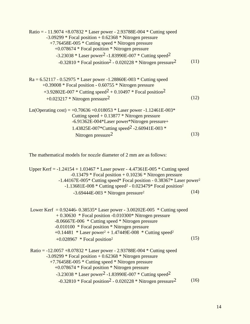
14

Ratio = - 11.9074 +8.07832 * Laser power - 2.93788E-004 * Cutting speed










Ln(Operating cost) = +0.70636 +0.018053 * Laser power -1.12461E-003*

Cutting speed + 0.13877 * Nitrogen pressure

-6.91362E-004*Laser power*Nitrogen pressure+

1.43825E-007*Cutting speed2 -2.60941E-003 *

Nitrogen pressure2 (13)

The mathematical models for nozzle diameter of 2 mm are as follows:

Upper Kerf = -1.24154 + 1.03467 * Laser power - 4.47361E-005 * Cutting speed


-1.44167E-005* Cutting speed* Focal position - 0.38367* Laser power2

-1.13681E-008 * Cutting speed2 - 0.023479* Focal position2


Lower Kerf = 0.92446- 0.38535* Laser power - 3.00202E-005 * Cutting speed

+ 0.30630 * Focal position -0.010300* Nitrogen pressure





Ratio = -12.0057 +8.07832 * Laser power - 2.93788E-004 * Cutting speed






15





Ln(Operating cost) =+1.26155 +0.013946 * Laser power

-1.12461E-003 * Cutting speed

+0.13975 * Nitrogen pressure

-6.91362E-004 * Laser power * Nitrogen pressure

+1.43825E-007 * Cutting speed2


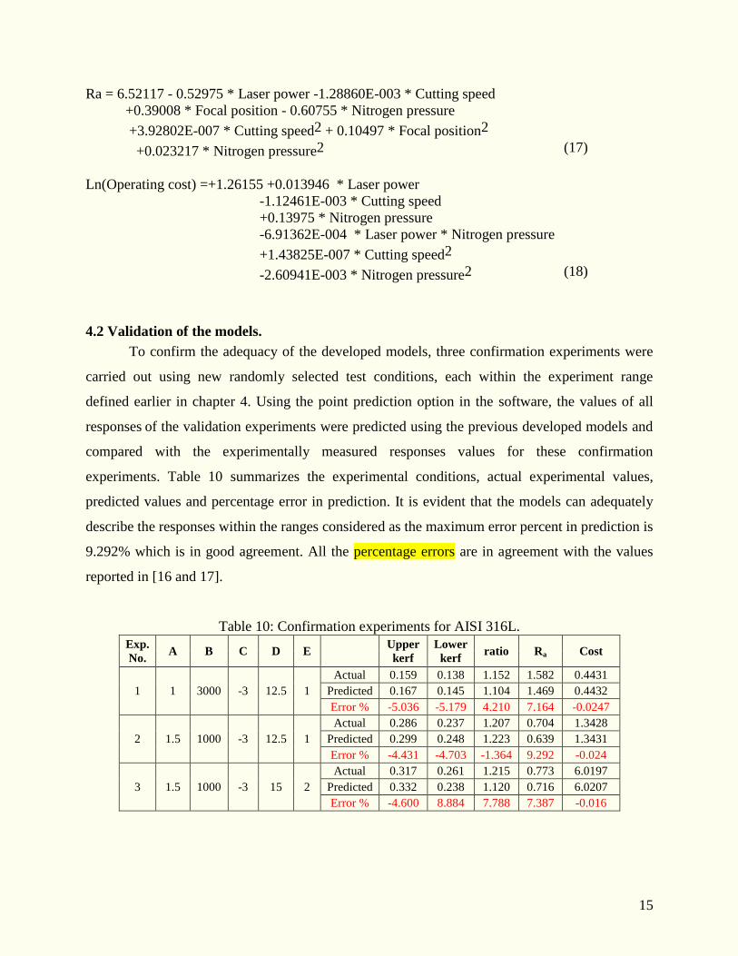
4.2 Validation of the models.

To confirm the adequacy of the developed models, three confirmation experiments were

carried out using new randomly selected test conditions, each within the experiment range

defined earlier in chapter 4. Using the point prediction option in the software, the values of all

responses of the validation experiments were predicted using the previous developed models and

compared with the experimentally measured responses values for these confirmation

experiments. Table 10 summarizes the experimental conditions, actual experimental values,

predicted values and percentage error in prediction. It is evident that the models can adequately

describe the responses within the ranges considered as the maximum error percent in prediction is

9.292% which is in good agreement. All the percentage errors are in agreement with the values

reported in [16 and 17].

Table 10: Confirmation experiments for AISI 316L.

Exp.

No. A B C D E

Upper

kerf

Lower

kerf ratio Ra Cost

1 1 3000 -3 12.5 1

Actual 0.159 0.138 1.152 1.582 0.4431

Predicted 0.167 0.145 1.104 1.469 0.4432

Error % -5.036 -5.179 4.210 7.164 -0.0247

2 1.5 1000 -3 12.5 1

Actual 0.286 0.237 1.207 0.704 1.3428

Predicted 0.299 0.248 1.223 0.639 1.3431

Error % -4.431 -4.703 -1.364 9.292 -0.024

3 1.5 1000 -3 15 2

Actual 0.317 0.261 1.215 0.773 6.0197

Predicted 0.332 0.238 1.120 0.716 6.0207

Error % -4.600 8.884 7.788 7.387 -0.016

16

4.3 Effect of process parameters on the responses

4.3.1 Upper kerf

The perturbation plot for the upper kerf width is shown in Fig. 1. The perturbation plot

helps to compare the effect of all factors at a particular point in the design space. This type of

display does not show the effect of interactions. The lines represent the behaviours of each factor,

while holding the others constant (i.e. centre point by default). In the case of more than one factor

this type of display could be used to find those factors that most affect the response. It is evident

from Fig. 1 that the upper kerf width increases as the laser power and gas pressure increase,

which agrees with [6, 7 and 8], yet above the centre values of both factors the upper kerf becomes

stable. However, the upper kerf width sharply decreases as the cutting speed increases. This is in

a good agreement with [7 and 8]. In the case of the focal point position, it is notable that as the

focal position increases up to the centre point (C = -3 mm) the upper kerf slightly increases, but,

as the focal point increases beyond this point the upper kerf begins to decrease.

Perturbation for AISI 316L

Deviation from Reference Point (Coded Units)

Upper

Kerf

, m

m

-1.000 -0.500 0.000 0.500 1.000

0.180

0.223

0.265

0.308

0.350

A

A

B

B

C

CD

D

Fig. 1: Perturbation plot showing the effect of process parameters on upper kerf width.

Table 11 presents the overall percentage change in the upper kerf width as a result of

changing each factor from its lowest value to its highest value while keeping the other factor at

their centre values. It is evident from Table 11 that the cutting speed is the main factor

influencing the upper kerf width, this result agrees with the results found in [7 and 8]. Fig. 2 is a

17

contour graph demonstrating the effect of both laser power and cutting speed on the upper kerf

width at two nozzle diameters 1 and 1.5 mm. In fact, all the investigated LBC parameters are

found to affect the upper kerf, and this outcome agrees with [4].

Table 11: Percentage change in upper kerf as each factor increases.

Factor Percentage change in upper kerf, %

Laser power Increases by 16.75

Cutting speed Decreases by 30.92

Focal position Decreases by 17.01

Nitrogen pressure Increases by 22.72

Nozzle diameter Increases by 11.56

1000.00 1500.00 2000.00 2500.00 3000.00

1.00

1.13

1.25

1.38

1.50

Upper Kerf, mm

B: cutting speed, mm/min

A: L

ase

r pow

er,

kW

0.190

0.210

0.2300.250

0.270

0.290

0.300

1000.00 1500.00 2000.00 2500.00 3000.00

1.00

1.13

1.25

1.38

1.50

Upper Kerf, mm


A: L

ase

r pow

er,

kW

0.210

0.230

0.2500.2700.290

0.310

0.330

0.300

0.320

(a) (b)

Fig. 2: Contours plot showing the effect of laser power and cutting speed on the upper kerf width

at different nozzle diameters (a) 1 mm and (b) 1.5 mm.

4.3.2 Lower kerf

It is clear from Fig. 3 that the lower kerf width increases as the laser power and the gas

pressure increase. However, this response decreases with the increase in the focal point position

up to the midpoint (i.e. -3 mm) and then starts to increase as the focal point position increases

from -3 mm towards -2 mm. This incident could be related to the interaction between the gas

18

pressure and the focal point position, which will be discussed later. Also, the lower kerf decreases

as the cutting speed increases this is in agreement with findings reported in [8].



Low

er

Kerf

, m

m

-1.000 -0.500 0.000 0.500 1.000

0.140

0.170

0.200

0.230

0.260

A

A

B

B

C

C

D

D

Fig. 3: Perturbation plot showing the effect of process parameters on lower kerf width.

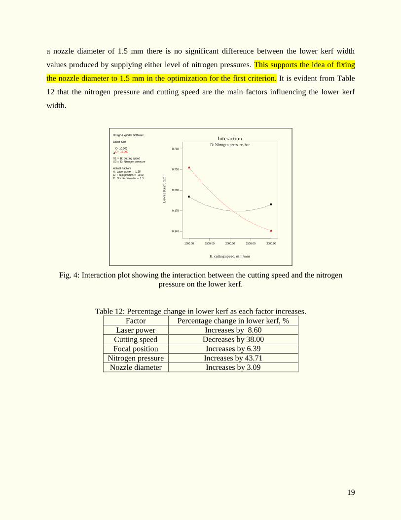
The interaction plots help the researchers to find the best parameter settings that lead to the

smaller possible lower kerf or the desirable response value. Fig. 4 demonstrates the interaction

effect between the cutting speed and nitrogen pressure on the lower kerf width. It is clear that at

low cutting speeds below 2100 mm/min a smaller lower kerf width of 0.170 mm could be

obtained if the lowest nitrogen pressure of 10 bar is used. On the other hand, at higher cutting

speeds above 2100 mm/min the smallest lower kerf width of 0.14 mm could be produced if the

highest nitrogen pressure of 15 bar was supplied. At cutting speeds of about 2100 mm/min both

levels of nitrogen pressure have the same effect on the lower kerf width. Fig. 5 shows the

interaction effect between the focal point position and the nitrogen pressure. It is evident that the

use of a wider laser beam (i.e. focal position of - 4 mm) leads a small lower kerf width of 0.17

only if the lowest gas pressure of 10 bar is applied. On the other hand, using a narrower laser

beam (i.e. focal position of - 2 mm) results in a small lower kerf width only when the highest

nitrogen pressure of 15 bar was applied. However, the nitrogen pressure would have the same

effect on the lower kerf width if a focal point position just above -3 mm was employed. Dilthey

et al. [9] have reported that exact adjustment of focal position and gas jet is essential, which

supports the above findings. It is clear from the interaction graph shown in Fig. 6 that when using

19

a nozzle diameter of 1.5 mm there is no significant difference between the lower kerf width

values produced by supplying either level of nitrogen pressures. This supports the idea of fixing

the nozzle diameter to 1.5 mm in the optimization for the first criterion. It is evident from Table

12 that the nitrogen pressure and cutting speed are the main factors influencing the lower kerf

width.

Design-Expert® Software

Lower Kerf

D- 10.000D+ 15.000

X1 = B: cutting speedX2 = D: Nitrogen pressure

Actual FactorsA: Laser power = 1.25C: Focal position = -3.00E: Nozzle diameter = 1.5

D: Nitrogen pressure, bar

1000.00 1500.00 2000.00 2500.00 3000.00

Interaction


Low

er

Kerf

, m

m

0.140

0.170

0.200

0.230

0.260

Fig. 4: Interaction plot showing the interaction between the cutting speed and the nitrogen

pressure on the lower kerf.

Table 12: Percentage change in lower kerf as each factor increases.

Factor Percentage change in lower kerf, %



Focal position Increases by 6.39



20


Lower Kerf

D- 10.000D+ 15.000

X1 = C: Focal positionX2 = D: Nitrogen pressure

Actual FactorsA: Laser power = 1.25B: cutting speed = 2000.00E: Nozzle diameter = 1.5


-4.00 -3.50 -3.00 -2.50 -2.00

Interaction

C: Focal position, mm

Low

er

Kerf

, m

m

0.140

0.170

0.200

0.230

0.260

Fig. 5: Interaction plot showing the interaction between the focal position and the nitrogen



Lower Kerf

D- 10.000D+ 15.000

X1 = E: Nozzle diameterX2 = D: Nitrogen pressure

Actual FactorsA: Laser power = 1.25B: cutting speed = 2000.00C: Focal position = -3.00


1 1.5 2

Interaction

E: Nozzle diameter

Low

er

Kerf

, m

m

0.120

0.155

0.190

0.225

0.260

Fig. 6: Interaction plot showing the interaction between the nozzle diameter and the nitrogen


21

4.3.3 Ratio

Fig. 7 is an interaction plot showing the influence of cutting speed and nitrogen pressure

on the ratio. It is apparent that by using cutting speeds below 1520 mm/min the ratio would be

less (close to one) if the highest nitrogen pressure of 15 bar was supplied. Above this value of

cutting speed the ratio would be less if the lowest nitrogen pressure of 10 bar was used. The same

trend was noticed as the nozzle diameter changed. From the interaction graph shown in Fig. 8 it

is obvious that by using focal position below -3.48 mm the ratio would be close to one if the

highest nitrogen pressure of 15 bar was used. Above -3.48 the ratio would be close to one as the

lowest nitrogen pressure of 10 bar was used. It is evident from Table 13 that the focal position

and nitrogen pressure are the main factors influencing the ratio. These findings are in fair

agreement with results reported in [10]. The results show that the range of the ratio lays between

0.94 and 1.93 for AISI316L. Therefore, a target ratio of one in this case will be a desirable goal

when searching for the optimal condition to obtain a square cut edge.


Ratio

D- 10.000D+ 15.000

X1 = B: cutting speedX2 = D: Nitrogen pressure

Actual FactorsA: Laser power = 1.25C: Focal position = -3.00E: Nozzle diameter = 1


1000.00 1500.00 2000.00 2500.00 3000.00

Interaction


Ratio

0.800

1.100

1.400

1.700

2.000

Fig. 7: Interaction plot showing the interaction between the cutting speed and the nitrogen

pressure on the ratio.

22

Table 13: Percentage change in ratio as each factor increases.

Factor Percentage change in ratio, %







Ratio

D- 10.000D+ 15.000

X1 = C: Focal positionX2 = D: Nitrogen pressure

Actual FactorsA: Laser power = 1.25B: cutting speed = 2000.00E: Nozzle diameter = 1


-4.00 -3.50 -3.00 -2.50 -2.00

Interaction

C: Focal position, mm

Ratio

0.600

0.950

1.300

1.650

2.000

Fig. 8: Interaction plot showing the interaction between the focal position and the nitrogen

pressure on the ratio.

4.3.4 Surface roughness

Fig. 9 is a perturbation plot showing the effect of all laser cutting parameters on the

roughness of the cut surface. It is evident from the results that the Ra value decreases as the laser

power, focal point position and nitrogen pressure increase; these finding are in agreement with

[11] and disagree with [12]. However, the Ra value starts to rise as the nitrogen pressure increases

above 13.4 bar as can be seen in Fig. 9. Moreover, the roughness decreases slightly as the cutting

speed increases up to 1505 mm/min, which agrees with [12]. Between 1505 – 1740 mm/min the

surface roughness values become stable, and then they remarkably increase as the cutting speed

increases above 1740 mm/min, which disagrees with [12]. The results confirm that the nozzle

diameter has no significant effect on the roughness of the cut surface in contrast to the apparent

23

results in Fig. 9. It is clear from Table 14 that the cutting speed, focal position and laser power

are the main factors influencing the cut surface roughness.

Table 14: Percentage change in roughness as each factor increases.

Factor Percentage change in Ra, %

Laser power Decreases by 33.39

Cutting speed Increases by 73.31


Nitrogen pressure Decreases by 15.52

Nozzle diameter No effect



Ra, um

-1.000 -0.500 0.000 0.500 1.000

0.400

0.750

1.100

1.450

1.800

A

A

B

B

C

C

D

D

Fig. 9: Perturbation plot showing the effect of process parameters on roughness.

4.3.5 Operating cost

The perturbation plot would help to compare the effect of all the factors at a particular

point in the design space. It is evident from Fig.10, that in the case of cutting speed, steep

curvatures indicate that the responses are too sensitive to this factor. Also, Fig. 10a-c

demonstrates the importance of the nozzle diameter with respect to the operating cost, while the

steep slopes in the case of laser power and nitrogen pressure indicate that the operating cost is

24

less sensitive to these factors. In addition, the results indicate that as the laser power, nitrogen

pressure and nozzle diameter increase the operating cost increases too. On the other hand, as the

cutting speed increases the operating cost decreases sharply. These results are intuitive because

more electrical power will be consumed as the laser power increases. Also, more gas will be

consumed as both the nitrogen pressure and the nozzle diameter increase. However, the cost will

decrease as the cutting speed increases due to the fact that the cutting will be performed in less

time, and consequently, less electrical power and nitrogen gas will be consumed. Fig. 10 is a

perturbation plot illustrating the above findings. It is apparent that the nozzle diameter, cutting

speed and nitrogen pressure are the key factors affecting the operating cost. Moreover, these

changes in the operating cost in terms of percentages are presented in Table 15 as each factor

increases from its lowest level to its highest level. It is clear that the focal position has no effect

on the operating cost.

On balance, it is evident from the above results for AISI316L that all the process

parameters considered in this research affect the quality features somehow. Furthermore, in some

cases, these parameter may interact in such a way that it becomes too hard to find the best cutting

conditions which lead to the desired quality features. Therefore, an overall optimization should be

performed for this material which would account for the minimization of the surface roughness,

kerf widths and operating cost etc, or the maximization of the cut edge squareness. It is notable

that the main factors affecting the operating cost are: nozzle diameter, cutting speed and minor

effect of laser power

25



Opera

ting c

ost

, E

uro

/m

-1.000 -0.500 0.000 0.500 1.000

0.4000

1.5750

2.7500

3.9250

5.1000

A A

B

BD

D



Opera

ting c

ost

, E

uro

/m

-1.000 -0.500 0.000 0.500 1.000

0.4000

1.5750

2.7500

3.9250

5.1000

A A

B

BD

D

(a) (b)



Opera

ting c

ost

, E

uro

/m

-1.000 -0.500 0.000 0.500 1.000

0.4000

1.5750

2.7500

3.9250

5.1000

A A

B

B

D

D

(c)

Fig. 10: Perturbation plot illustrating the effect of process factors on operating cost at different

nozzle diameters (a) 1 mm, (b) 1.5 mm and (c) 2 mm.

Table 15: Percentage change in cost as each factor increases.

Factor Percentage change in cost, %



Focal position No effect



26

5. OPTIMIZATION

Laser cutting is a multi-input and multi-output process that needs to be assessed carefully

in order to achieve the most desirable results. Planning the fabrication of parts based on quality of

the final cut surface alone may have important cost implications, which should be evaluated.

Based on the previously presented results and discussion it is clear that there are many factors

and their interactions, which affect the process. Thus, an in-depth optimization is required. To run

any optimization it is important to know the following: the effect of each factor and its interaction

effect with the other factors on the responses, the output of the process (i.e. responses) and finally

the desirable criterion (i.e. the goal). In the numerical optimization for this research two criteria

were used. The difference between these two criteria is that in the first criterion there were no

restrictions on the process input parameters and the output quality features were set to achieve the

highest quality in terms of surface roughness and cut edge perpendicularity (referring to this

criterion as Quality). In the second criterion, the cost of the cutting is the main issue;

consequently, some restrictions have been put on the process input parameters which have an

effect on the operating cost. Also, regarding the second criterion, the operating cost was set to be

a minimum with no restrictions on the other responses (referring to this criterion as Cost). This

multi-responses optimization is solved via the desirability approach explained earlier in chapter 3,

which is built in the Design expert software. Two types of optimization layout are available in

Design expert. The first one, the numerical optimization feature, which finds a point or more in

the factors domain that, would maximize the overall desirability (i.e. objective function). The

second one, the graphical optimization, where the optimal range of each response has to be

brought from the numerical optimization results in order to present them graphically. The

graphical optimization allows visual selection of the optimal cutting conditions according to

certain criterion. Graphical optimization results in plots called overlay plots. These plots are

extremely practical for technical use at the workshop and help the operator to choose the optimal

values of the laser cutting parameters to achieve the desirable response values for each material.

The green/shaded areas on the overlay plots are the regions that meet the proposed criteria.

For this material the two optimization criteria are presented in Table 16. As seen in Table

16, that each factor and response have allocated a specific goal and importance. The nozzle

27

diameter was set at 1.5 mm. This value was chosen because it was found to be the best nozzle

diameter that would lead to kerf widths close to each other, and consequently, a square cut edge.

5.1 Numerical optimization

Table 17 shows the optimal setting of the process parameters and the corresponding

response values for both criteria for 2 mm AISI316L. It is noticeable that to obtain the superior

quality cut with predicted ratio as close as possible to one and Ra 0.405 m. The laser power

has to be 1.49 kW with cutting speed between 1538-1661 mm/min, a focal point position of -2.02

mm, nitrogen pressure of around 11.4 bar and nozzle diameter of 1.5 mm have to be applied.

Alternatively, if the reduction in the cutting cost is essential, it is confirmed that, a laser power of

1.02 kW has to be applied with cutting speed from 1900 to 2968 mm/min, a focal point position

ranged from -3.92 mm to -2.85 mm, nitrogen pressure ranged between 10.4-12.9 bar and a nozzle

diameter of 1 mm have to be used. It is clear that the roughness of cut section produced by using

the setting of the first criterion is on average 65.8% smoother than the one produced by using the

conditions of the second criterion. On the other hand, the cutting operating cost in the second

criterion is on average 71% cheaper than that of the first criterion.

5.2 Graphical optimization

As mentioned earlier the range of each response has been chosen from the numerical

optimization results in Table 17. These ranges were brought into the graphical optimization.

Figures 11 and 12 show green areas which are the regions that comply with the first and second

criteria respectively.

28

Table 16: Criteria for numerical optimization of AISI316L.

Factor or response First criterion (Quality) Second criterion (Cost)

Goal Importance Goal Importance

Laser power Is in range 3 Minimize 5

Cutting speed Is in range 3 Maximize 5

Focal position Is in range 3 Is in range 3

N2 pressure Is in range 3 Minimize 3

Nozzle Diameter Equal to 1.5 3 Minimize 5

Upper Kerf Is in range 3 Is in range 3

Lower Kerf Is in range 3 Is in range 3

Ratio Target to 1 5 Is in range 3

Roughness Minimize 5 Is in range 3

Operating cost Is in range 3 Minimize 5

Table 17: Optimal cutting conditions as obtained by Design-Expert for 2 mm thick AISI316L.

No.

A,

kW

B,

mm/min

C,

mm

D,

bar

E,

mm

Upper

kerf,

mm

Lower

kerf,

mm

Ratio Ra,

mm

Cost,

€/m Desirability

1st c

rite

rion

Qual

ity

1 1.49 1635 -2.02 11.3 1.5 0.26 0.251 1 0.409 1.66 1

2 1.49 1636 -2.01 11.4 1.5 0.26 0.251 1 0.402 1.67 1

3 1.49 1650 -2.01 11.4 1.5 0.26 0.251 1 0.401 1.66 1

4 1.49 1661 -2.02 11.4 1.5 0.258 0.25 1 0.409 1.63 1

5 1.49 1538 -2 11.4 1.5 0.265 0.254 1 0.409 1.78 1

2n

d c

rite

rion

Cost

1 1.02 2575 -3.32 11.7 1 0.198 0.145 1.243 1.195 0.48 0.8311

2 1.22 2968 -3.92 11.4 1 0.208 0.146 1.099 1.685 0.41 0.7927

3 1.03 2106 -3.11 11.1 1 0.21 0.151 1.31 0.919 0.57 0.7754

4 1.02 2831 -3.08 12.9 1 0.19 0.15 1.246 1.303 0.48 0.7721

5 1.04 1900 -2.85 10.4 1 0.198 0.154 1.199 0.878 0.60 0.7625

29

Design-Expert® SoftwareOriginal ScaleOverlay Plot

Upper KerfLower KerfRatioRaOperating cost

X1 = D: Nitrogen pressureX2 = B: cutting speed

Actual FactorsA: Laser power = 1.49C: Focal position = -2.01E: Nozzle diameter = 1.5

11.36 11.37 11.38 11.39 11.39

1624.33

1630.95

1637.56

1644.18

1650.79

Overlay Plot for AISI316L


B:

cutt

ing

sp

eed

, mm

/min

Upper Kerf: 0.260

Ratio: 0.999Ratio: 1.000

Ra: 0.409

Fig. 11: Overlay plot shows the region of optimal cutting condition based on the first

criterion for 2 mm AISI316L.

Design-Expert® SoftwareOriginal ScaleOverlay Plot

Upper KerfLower KerfRatioRaOperating cost

X1 = D: Nitrogen pressureX2 = B: cutting speed

Actual FactorsA: Laser power = 1.02C: Focal position = -3.30E: Nozzle diameter = 1

10.37 11.16 11.95 12.73 13.52

1851.14

2107.17

2363.21

2619.25

2875.28

Overlay Plot for AISI316L


B:

cutt

ing

sp

eed

, mm

/min

Upper Kerf: 0.198

Upper Kerf: 0.208Lower Kerf: 0.145

Lower Kerf: 0.154Ratio: 1.099

Ratio: 1.310

Ra: 0.878

Operating cost: 0.4130

Operating cost: 0.5990

Fig. 12: Overlay plot shows the region of optimal cutting condition based on the second

criterion for 2 mm AISI316L.

30

CONCLUSIONS

The following points can be concluded from this work within the factors limits:

1. The upper kerf width increases as the laser power, nitrogen pressure and nozzle

diameter increase, and it decreases as the cutting speed and focal position

increase. However, the cutting speed is the main factor affecting the upper kerf.

2. The laser power, nitrogen pressure and focal position have a positive effect on the

lower kerf width. While, the cutting speed has a negative effect.

3. The ratio increases as the laser power, nitrogen pressure and nozzle diameter

increase, and it decreases as the cutting speed and focal position increases.

4. The roughness value increases as the cutting speed increases and it decreases as

the other parameters increases. However, the nozzle diameter has no significant

effect on the roughness.

5. The optimal cutting setting for AISI316L are laser power of 1.49 kW, cutting

speed between 1538 and 1661 mm/min, a focal point position of - 2.02 mm,

nitrogen pressure of around 11.4 bar and nozzle diameter of 1.5 mm if the quality

is important. The cut section roughness is on average 65.8% smoother if this

setting was applied.

6. The economical optimal settings are laser power of 1.02 kW, cutting speed from

1900 to 2968 mm/min, a focal point position ranged from -3.92 mm to -2.85 mm,

nitrogen pressure ranged between 10.4 and 12.9 bar and a nozzle diameter of 1

mm.

7. A reduction of about 71% in the cutting operating cost could be achieved, if the

economical setting is considered.

Acknowledgments

The authors wish to thank Mr. Martin Johnson the laser expert in DCU and the School of

Mechanical and Manufacturing Engineering, Dublin City University for the financial

support of this work.

31

REFERENCE

[1] J. Powell, CO2 Laser Cutting, 2nd

Edition, Springer-Verlag Berlin Heidelberg, New

York, (1998).

[2] W. M. Steen, Laser Material processing, Springer, London, 1991.

[3] S. L. Chen, The effects of gas composition on the CO2 laser cutting of mild steel, J.

Material Process Technology, Vol. 73, 1998, pp. 147–159.

[4] K. A. Ghany, M. Newishy, Cutting of 1.2mm thick austenitic stainless steel sheet

using pulsed and CW Nd:YAG laser, J. of Materials Processing Technology, Vol.

168, 2005, pp. 438–447.

[5] S. L. Chen, The effects of high-pressure assistant-gas flow on high-power CO2 laser

cutting, J. Material Processing Technology, Vol. 88, 1999, pp. 57–66.

[6] I. Uslan, CO2 laser cutting: kerf width variation during cutting, Proc. Of IMechE, Vol.

219 part B, J. of Engineering Manufacture, 2005, pp. 572-577.

[7] B. S. Yilbas, Effect of process parameters on the kerf width during the laser cutting

process, Proc Instn Mech Engrs, Vol. 215 part B, J. of Engineering Manufacture,

2001, pp. 1357-1365.

[8] B. S. Yilbas, Laser cutting quality and thermal efficiency analysis, J. of Materials

Processing Technology, Vol. 155-156, 2004, pp. 2106-2115.

[9] U. Dilthey, M. Faerber and J. Weick, Laser cutting of steel-cut quality depending on

cutting parameters, J. of Welding in the World, Vol. 30, No. 9/10, 1992, pp. 275-278.

[10] B. S. Yilbas and M. Rashid, CO2 laser cutting of Incoloy 800 HT alloy and its

quality assessment, J. of Laser in Engineering, Vol. 12, No. 2, 2002, pp. 135-145.

[11] M. Radovanovic and P. Dasic, Research on surface roughness by laser cut, the

Annals of University “Dunarea De Jos” of Galati Fascicle VII, ISSN 1221-4590,

Tribology, 2006, pp. 84-88.

[12] R. Neimeyer, R. N. Smith and D. A. Kaminski, Effects of operating parameters on

surface quality for laser cutting of mild steel, J. of Engineering for Industry, Vol.

115, 1993, pp. 359-362.

[13] A. K. Dubey and V. Yadava, Multi-objective optimization of laser beam cutting

process, Optics and Laser Technology, Vol. 40, No. 3, (2008), pp. 562–570.

32

[14] A. K. Dubey and V. Yadava, Multi-objective optimization of Nd:YAG laser cutting

of nickel-based superalloy sheet using orthogonal array with principal component

analysis, Optics and Laser Engineering, Vol. 46, (2008), pp. 124–132.

[15] B. S. Yilbas, Laser cutting of thick sheet metals: Effects of cutting parameters on

kerf size variations, J. of Materials Processing Technology, Vol. 201, No. 1-3, 26

May (2008), pp. 285-290.

[16] H. A. Eltawahni, A.G. Olabi, K. Y. Benyounis, Effect of process parameters and

optimization of CO2 laser cutting of ultra high-performance polyethylene, Materials

& Design, Volume 31, Issue 8, September 2010, Pages 4029-4038.

[17] H. A. Eltawahni, A.G. Olabi, K. Y. Benyounis, Investigating the CO2 laser cutting

parameters of MDF wood composite material, Journal of optics and Laser

Technology, Volume 43, Issue 3, April 2011, pp. 648-659.

[18] H. A. Eltawahni, A. G. Olabi, K. Y. Benyounis, Assessment and Optimization of

CO2 Laser Cutting Process of PMMA, AIP Conference Proceedings, v 1315, 1553-8,

2011; ISSN: 0094-243X; Conference: International Conference on Advances in

Materials and Processing Technologies (AMPT 2010), 24-27 Oct. 2010, Paris,

France; Publisher: American Institute of Physics, USA.

[19] I. A. Choudhury and S. Shirley, laser cutting of polymeric materials: An

experimental investigation, journal of Optics and Laser Technology, Vol. 42, 2010,

pp. 503-508.

[20] Chen-Hao Li, Ming-Jong Tsai, Ciann-Dong Yang, Study of optimal laser parameters

for cutting QFN packages by Taguchi's matrix method, Optics & Laser Technology,

Volume 39, Issue 4, June 2007, Pages 786-795.

[21] A. Sharma, V. Yadava, Modelling and optimization of cut quality during pulsed

Nd:YAG laser cutting of thin Al-alloy sheet for straight profile, Optics & Laser

Technology, In Press, Corrected Proof, Available online 20 July 2011.

[22] K. Y. Benyounis and A.G. Olabi, Optimization of different welding process using

statistical and numerical approaches- A reference guide, Journal of Advances in

Engineering Software, 39, (2008) 483-496.

[23] A. Ruggiero, L. Tricarico, A.G. Olabi, K. Y. Benyounis, Weld-bead profile and

costs optimization of the CO2 dissimilar laser welding process of low carbon steel

33

and austenitic steel AISI316, Optics & Laser Technology, Volume 43, Issue 1,

February 2011, Pages 82-90.

[24] K. Y. Benyounis, A.G. Olabi and M. S. J. Hashmi, Multi-response optimization of

CO2 laser-welding process of austenitic stainless steel, Optics & Laser Technology,

40 (1) (2008) 76-87.

[25] A. G. Olabi, G. Casalion, K. Y. Benyounis, and M. S. J. Hashmi, Minimization of

the residual stress in the heat affected zone by means of numerical methods, J. of

Materials & Design, Vol. 28, No. 8, 2007, pp. 2295-2302.

effect of co2 laser cutting process...

Documents