effect of boundary conditions on the axial compression … · · 2013-04-10american institute of...

American Institute of Aeronautics and Astronautics

1

Effect of Boundary Conditions on the Axial Compression Buckling of Homogeneous Orthotropic Composite Cylinders

in the Long Column Range

Martin M. Mikulas, Jr.1 National Institute of Aerospace, Hampton, VA 23666

Michael P. Nemeth2 NASA Langley Research Center, Hampton, VA 23681

Leonard Oremont3 Lockheed Martin Corp., Hampton, VA 23681

and

Dawn C. Jegley4 NASA Langley Research Center, Hampton, VA 23681

Buckling loads for long isotropic and laminated cylinders are calculated based on Euler, Flügge and Donnell’s equations. Results from these methods are presented using simple parameters useful for fundamental design work. Buckling loads for two types of simply supported boundary conditions are calculated using finite element methods for comparison to select cases of the closed form solution. Results indicate that relying on Donnell theory can result in an over-prediction of buckling loads by as much as 40% in isotropic materials.

Nomenclature A11, A12, A22, A66, A16, A26 = Membrane stiffnesses of laminated-composite cylinder, lb/in. B11, B12, B22, B66, B16, B26 = Membrane-bending coupling stiffnesses of laminated-composite cylinder, lb

Bij( ) = Differential operators defined in Eqs. (A10)

cx = Nondimensional buckling coefficient defined by Eqs. (2) and (3) C0, C1, C2 = Coefficients defined by Eqs. (A17) D11, D12, D22, D66, D16, D26 = Bending stiffnesses of laminated-composite cylinder, in-lb E = Elastic modulus of isotropic material, psi

E = Effective modulus of quasi-isotropic laminates, psi E1, E2, G12 = Lamina elastic moduli, psi Ex, Ey, Gxy = Effective laminate elastic moduli, psi k = Thinness parameter (see Fig. 2) Kij = Stiffnesses defined by Eqs. (A14) L = Cylinder length, in. (see Fig. 5)

L = Nondimensional buckling parameter defined by Eqs. (1) and (4)

Lij( ) = Differential operators defined in Eqs. (A8)

m = Number of axial half waves in buckle pattern (see Eqs. (A12)) MPC = Multiple Point Constraint

1 Senior Research Fellow, Fellow, AIAA, 100 Exploration Way. 2 Senior Aerospace Engineer, Associate Fellow, AIAA, Structural Mechanics and Concepts Branch, mail stop 190. 3 Senior Aerospace Engineer, Structural Mechanics and Concepts Branch, mail stop 460. 4 Senior Aerospace Engineer, Associate Fellow, AIAA, Structural Mechanics and Concepts Branch, mail stop 190.

https://ntrs.nasa.gov/search.jsp?R=20110009992 2018-07-07T02:43:26+00:00Z


2

Mxx, Myy, Mxy = Bending stress resultants, lb/in. (see Eqs. (A3)) n = Number of circumferential waves in buckle pattern (see Eqs. (A12)) N, Ncr = Applied compressive end running load and value at buckling, respectively, lb/in. Nxx, Nyy, Nxy = Membrane stress resultants, lb/in. (see Eqs. (A3))

Nxx

(0)

, Nyy

(0)

, Nxy

(0) = Prebuckling membrane stress resultants, lb/in. (see Eqs. (A5))

crp, p = Loading parameters (see Eq. (A7))

Pcr = Critical buckling load, lb R, t = Cylinder radius and wall thickness, respectively, in. (see Fig. 5) S1, S2 = Simply supported boundary conditions u(x, y), v(x, y), w(x, y) = Axial, circumferential and radial displacement fields, in. u, v, w = Displacement-field amplitudes (see Eq. (A12)) x, y, z = Cylinder coordinates (see Fig. 5) εxx

o , εyy

o , γxy

o = Membrane strains

κ xx

o, κ yy

o, κ xy

o = Bending strains, 1/in.

σxx, σyy, σxy = Stresses, psi σDonnell, σFlügge = Buckling stress based on the Donnell and Flügge equations, psi σEuler = Buckling stress based on the Euler column buckling formula, psi θ = Fiber orientation angle, degrees ν = Poisson’s ratio of isotropic materials ν12 = Poisson’s ratio of composite lamina νxy, νyx = Effective Poisson’s ratios of composite laminate

I. Introduction ecause of the high cost per pound associated with the launch of lunar and other planetary vehicles, the design of the structural

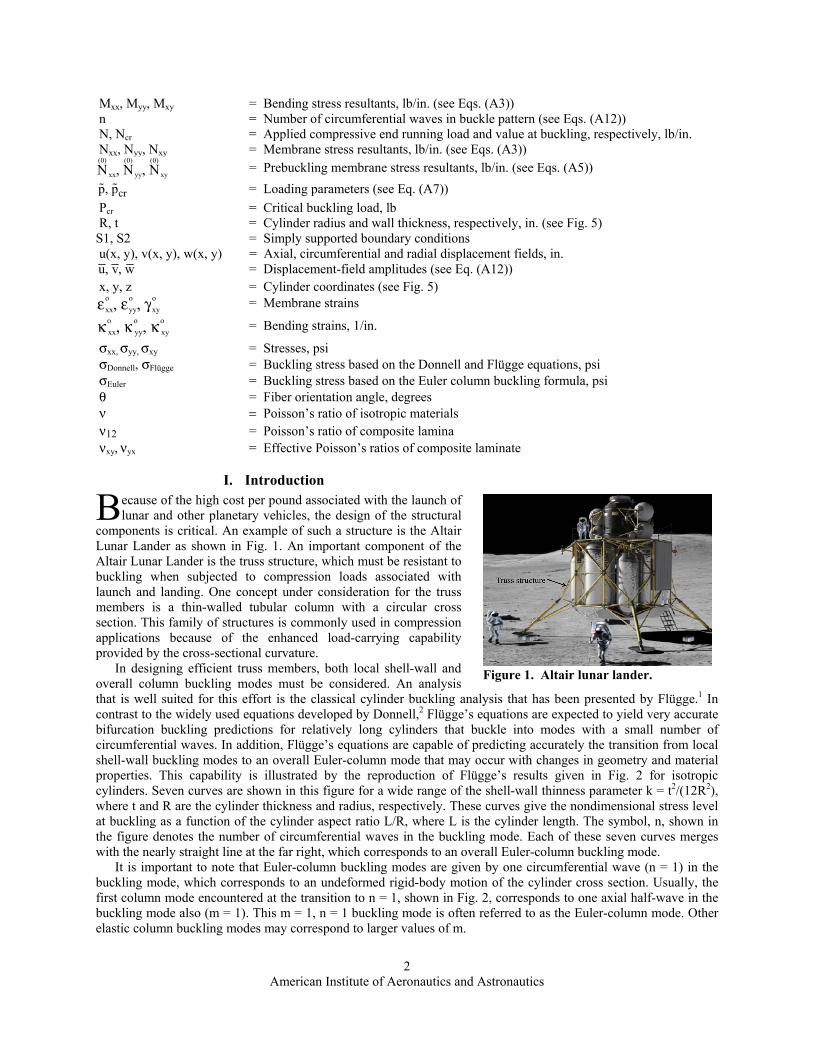
components is critical. An example of such a structure is the Altair Lunar Lander as shown in Fig. 1. An important component of the Altair Lunar Lander is the truss structure, which must be resistant to buckling when subjected to compression loads associated with launch and landing. One concept under consideration for the truss members is a thin-walled tubular column with a circular cross section. This family of structures is commonly used in compression applications because of the enhanced load-carrying capability provided by the cross-sectional curvature.

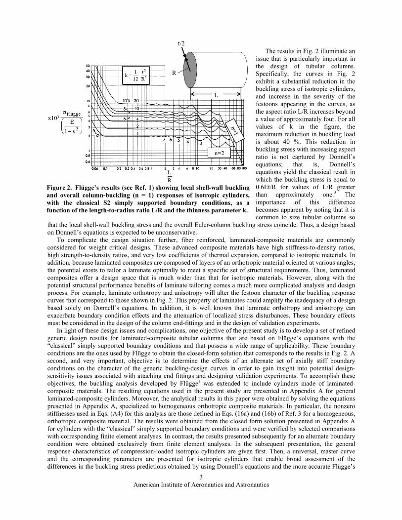
In designing efficient truss members, both local shell-wall and overall column buckling modes must be considered. An analysis that is well suited for this effort is the classical cylinder buckling analysis that has been presented by Flügge.1 In contrast to the widely used equations developed by Donnell,2 Flügge’s equations are expected to yield very accurate bifurcation buckling predictions for relatively long cylinders that buckle into modes with a small number of circumferential waves. In addition, Flügge’s equations are capable of predicting accurately the transition from local shell-wall buckling modes to an overall Euler-column mode that may occur with changes in geometry and material properties. This capability is illustrated by the reproduction of Flügge’s results given in Fig. 2 for isotropic cylinders. Seven curves are shown in this figure for a wide range of the shell-wall thinness parameter k = t2/(12R2), where t and R are the cylinder thickness and radius, respectively. These curves give the nondimensional stress level at buckling as a function of the cylinder aspect ratio L/R, where L is the cylinder length. The symbol, n, shown in the figure denotes the number of circumferential waves in the buckling mode. Each of these seven curves merges with the nearly straight line at the far right, which corresponds to an overall Euler-column buckling mode.

It is important to note that Euler-column buckling modes are given by one circumferential wave (n = 1) in the buckling mode, which corresponds to an undeformed rigid-body motion of the cylinder cross section. Usually, the first column mode encountered at the transition to n = 1, shown in Fig. 2, corresponds to one axial half-wave in the buckling mode also (m = 1). This m = 1, n = 1 buckling mode is often referred to as the Euler-column mode. Other elastic column buckling modes may correspond to larger values of m.

B

Figure 1. Altair lunar lander.


3

The results in Fig. 2 illuminate an issue that is particularly important in the design of tubular columns. Specifically, the curves in Fig. 2 exhibit a substantial reduction in the buckling stress of isotropic cylinders, and increase in the severity of the festoons appearing in the curves, as the aspect ratio L/R increases beyond a value of approximately four. For all values of k in the figure, the maximum reduction in buckling load is about 40 %. This reduction in buckling stress with increasing aspect ratio is not captured by Donnell’s equations; that is, Donnell’s equations yield the classical result in which the buckling stress is equal to 0.6Et/R for values of L/R greater than approximately one.3 The importance of this difference becomes apparent by noting that it is common to size tubular columns so

that the local shell-wall buckling stress and the overall Euler-column buckling stress coincide. Thus, a design based on Donnell’s equations is expected to be unconservative.

To complicate the design situation further, fiber reinforced, laminated-composite materials are commonly considered for weight critical designs. These advanced composite materials have high stiffness-to-density ratios, high strength-to-density ratios, and very low coefficients of thermal expansion, compared to isotropic materials. In addition, because laminated composites are composed of layers of an orthotropic material oriented at various angles, the potential exists to tailor a laminate optimally to meet a specific set of structural requirements. Thus, laminated composites offer a design space that is much wider than that for isotropic materials. However, along with the potential structural performance benefits of laminate tailoring comes a much more complicated analysis and design process. For example, laminate orthotropy and anisotropy will alter the festoon character of the buckling response curves that correspond to those shown in Fig. 2. This property of laminates could amplify the inadequacy of a design based solely on Donnell’s equations. In addition, it is well known that laminate orthotropy and anisotropy can exacerbate boundary condition effects and the attenuation of localized stress disturbances. These boundary effects must be considered in the design of the column end-fittings and in the design of validation experiments.

In light of these design issues and complications, one objective of the present study is to develop a set of refined generic design results for laminated-composite tubular columns that are based on Flügge’s equations with the “classical” simply supported boundary conditions and that possess a wide range of applicability. These boundary conditions are the ones used by Flügge to obtain the closed-form solution that corresponds to the results in Fig. 2. A second, and very important, objective is to determine the effects of an alternate set of axially stiff boundary conditions on the character of the generic buckling-design curves in order to gain insight into potential design-sensitivity issues associated with attaching end fittings and designing validation experiments. To accomplish these objectives, the buckling analysis developed by Flügge1 was extended to include cylinders made of laminated-composite materials. The resulting equations used in the present study are presented in Appendix A for general laminated-composite cylinders. Moreover, the analytical results in this paper were obtained by solving the equations presented in Appendix A, specialized to homogeneous orthotropic composite materials. In particular, the nonzero stiffnesses used in Eqs. (A4) for this analysis are those defined in Eqs. (16a) and (16b) of Ref. 3 for a homogeneous, orthotropic composite material. The results were obtained from the closed form solution presented in Appendix A for cylinders with the “classical” simply supported boundary conditions and were verified by selected comparisons with corresponding finite element analyses. In contrast, the results presented subsequently for an alternate boundary condition were obtained exclusively from finite element analyses. In the subsequent presentation, the general response characteristics of compression-loaded isotropic cylinders are given first. Then, a universal, master curve and the corresponding parameters are presented for isotropic cylinders that enable broad assessment of the differences in the buckling stress predictions obtained by using Donnell’s equations and the more accurate Flügge’s

Figure 2. Flügge’s results (see Ref. 1) showing local shell-wall buckling and overall column-buckling (n = 1) responses of isotropic cylinders, with the classical S2 simply supported boundary conditions, as a function of the length-to-radius ratio L/R and the thinness parameter k.


4

equations. A similar set of universal curves for homogeneous orthotropic cylinders are then presented for a wide range of laminate orthotropy, along with selected validation results obtained from finite element analyses. Results for this particular class of laminated-composites provide a good first approximation in the design of cylinders with more general wall constructions. Then, using the universal curves, finite element results are presented that indicate the effects of enforcing additional axial restraint on the buckling response of selected laminated-composite cylinders.

II. Response Characteristics of Isotropic Cylinders To gain insight into the commonality of the response trends illustrated by the seven curves shown in Fig. 2, an

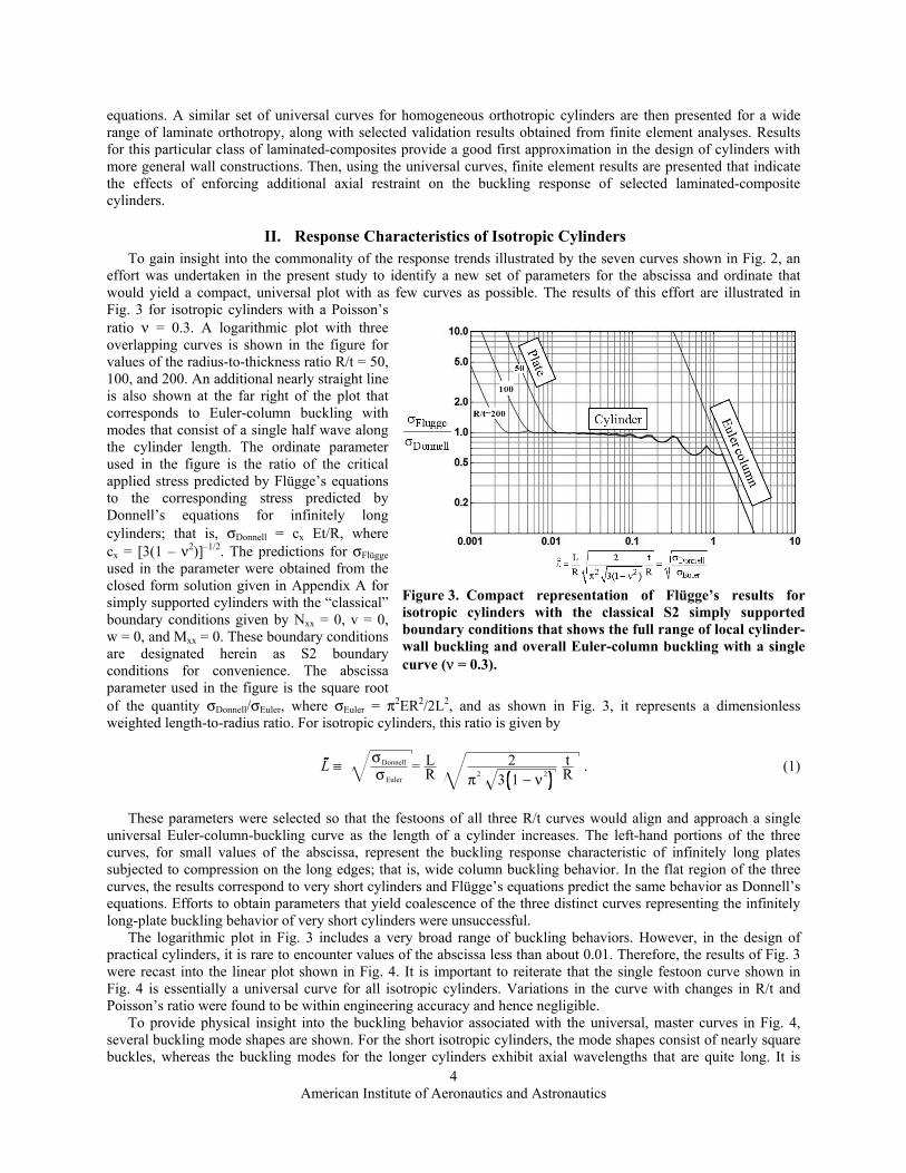
effort was undertaken in the present study to identify a new set of parameters for the abscissa and ordinate that would yield a compact, universal plot with as few curves as possible. The results of this effort are illustrated in Fig. 3 for isotropic cylinders with a Poisson’s ratio ν = 0.3. A logarithmic plot with three overlapping curves is shown in the figure for values of the radius-to-thickness ratio R/t = 50, 100, and 200. An additional nearly straight line is also shown at the far right of the plot that corresponds to Euler-column buckling with modes that consist of a single half wave along the cylinder length. The ordinate parameter used in the figure is the ratio of the critical applied stress predicted by Flügge’s equations to the corresponding stress predicted by Donnell’s equations for infinitely long cylinders; that is, σDonnell = cx Et/R, where cx = [3(1 – ν2)]–1/2. The predictions for σFlügge used in the parameter were obtained from the closed form solution given in Appendix A for simply supported cylinders with the “classical” boundary conditions given by Nxx = 0, v = 0, w = 0, and Mxx = 0. These boundary conditions are designated herein as S2 boundary conditions for convenience. The abscissa parameter used in the figure is the square root of the quantity σDonnell/σEuler, where σEuler = π2ER2/2L2, and as shown in Fig. 3, it represents a dimensionless weighted length-to-radius ratio. For isotropic cylinders, this ratio is given by

L ≡ σDonnell

σEuler

= LR

2π2 3 1 − ν2

tR

. (1)

These parameters were selected so that the festoons of all three R/t curves would align and approach a single universal Euler-column-buckling curve as the length of a cylinder increases. The left-hand portions of the three curves, for small values of the abscissa, represent the buckling response characteristic of infinitely long plates subjected to compression on the long edges; that is, wide column buckling behavior. In the flat region of the three curves, the results correspond to very short cylinders and Flügge’s equations predict the same behavior as Donnell’s equations. Efforts to obtain parameters that yield coalescence of the three distinct curves representing the infinitely long-plate buckling behavior of very short cylinders were unsuccessful.

The logarithmic plot in Fig. 3 includes a very broad range of buckling behaviors. However, in the design of practical cylinders, it is rare to encounter values of the abscissa less than about 0.01. Therefore, the results of Fig. 3 were recast into the linear plot shown in Fig. 4. It is important to reiterate that the single festoon curve shown in Fig. 4 is essentially a universal curve for all isotropic cylinders. Variations in the curve with changes in R/t and Poisson’s ratio were found to be within engineering accuracy and hence negligible.

To provide physical insight into the buckling behavior associated with the universal, master curves in Fig. 4, several buckling mode shapes are shown. For the short isotropic cylinders, the mode shapes consist of nearly square buckles, whereas the buckling modes for the longer cylinders exhibit axial wavelengths that are quite long. It is

Figure 3. Compact representation of Flügge’s results for isotropic cylinders with the classical S2 simply supported boundary conditions that shows the full range of local cylinder-wall buckling and overall Euler-column buckling with a single curve (ν = 0.3).


5

important to note that this class of cylinders exhibits unstable bifurcations and, as a result, the buckling mode is not the deformed shape that the cylinder exhibits when postbuckling equilibrium is first achieved. Moreover, often several bifurcation modes correspond to buckling loads that are nearly equal. For the very long cylinders, the buckling mode is a column-like move with one axial half wave. This mode corresponds to m = 1 and n = 1 in Eqs. (A12).

A common design approach for moderately long cylindrical structures is to size the cylinder such that local wall buckling and Euler-column buckling coincide. This design condition would be represented by the coordinates (1,1) on the chart in Fig. 4 for buckling results based on Donnell’s equations. As can be seen from the chart, Flügge’s equations

predict a buckling stress about 40% lower than that predicted by Donnell’s equations. The chart coordinates that correspond to coincident cylinder local wall and column buckling based on Flügge’s equations are approximately (1.3,0.6).

III. Universal Curves for Orthotropic Cylinders Curves similar to those shown in Fig. 2 for isotropic cylinders

were obtained for laminated-composite cylinders made of a graphite-epoxy material with lamina elastic moduli E1 = 21.4 Msi and E2 = 1.46 Msi, a shear modulus G12 = 0.69 Msi, and a major Poisson’s ratio ν12 = 0.3. Only laminate constructions that are effectively homogeneous and orthotropic were considered because of their basic importance in the design of more complicated wall constructions. Specifically, laminate walls that consist of three families of plies were considered. The three families are 0-degree, 90-degree, and ±θ angle plies where the angle θ is measured from a cylinder generator, as shown in Fig. 5. In addition, it is presumed that a laminate wall contains enough plies to be effectively homogeneous and exhibits no form of anisotropy. Moreover, the principal axes of orthotropy are taken to coincide with the x- and y- cylinder coordinate axes at each point of the cylinder mid-surface. A detailed discussion of these laminate constructions is given in Ref. 3.

After examining the curves obtained for the orthotropic cylinders, an effort was undertaken to identify a set of parameters for the abscissa and ordinate that would also yield a compact, universal plot like that shown in Fig. 4 for isotropic cylinders. Figures 6a and 6b illustrate the results of this effort for orthotropic cylinders with various percentages of 0-degree, 90-degree, and ±45-degree plies. Five curves for local wall buckling are shown in Fig. 6a for cylinders that buckle into asymmetric modes (n ≠ 0). The lowermost black curve corresponds to a quasi-isotropic laminate with 25% 0-degree plies, 50% ±45-degree plies, and 25% 90-degree plies. Similarly, the green curve corresponds to a laminate with 50% 0-degree plies, 40% ±45-degree plies, and 10% 90-degree plies. The red curve corresponds to a laminate with 60% 0-degree plies, 30% ±45-degree plies, and 10% 90-degree plies. The blue curve is for 70% 0-degree plies, 20% ±45-degree plies, and 10% 90-degree plies. Lastly, the gold curve corresponds to a laminate with 90% 0-degree plies and 10% 90-degree plies, and the rightmost blue curve corresponds to Euler-column buckling. Altogether, these laminate constructions represent a very broad range of orthotropy. The buckling behaviors of these laminates are discussed in detail in the text associated with Figs. 25–33 of Ref. 3.

Figure 4. Master curves and buckling mode shapes for isotropic cylinders with the classical S2 simply supported boundary conditions.

Figure 5. Cylinder geometry and ply orientation.


6

a) b) Figure 6. Master curves showing buckling behavior of laminated-composite cylinders with the classical S2 simply supported boundary conditions. a) Curves for asymmetric buckling modes (n ≠ 0). b) Curves for axisymmetric buckling modes (n = 0).

Two additional curves are shown in Fig. 6b in addition to the blue Euler-column-buckling curve, for cylinders

that buckle into axisymmetric modes (n = 0). The solid black curve is for quasi-isotropic laminates with 25% 0-degree plies, 50% ±45-degree plies, and 25% 90-degree plies. The dashed curve shown in Fig. 6b corresponds to 100% ±45-degree plies. The ordinate parameter used in Figs. 6a and 6b is the ratio of the critical applied stress predicted by Flügge’s equations to the corresponding stress predicted by Donnell’s equations for infinitely long cylinders. However, for the orthotropic cylinders σDonnell is that given in Eqs. (43) of Ref. 3. Specifically,

σDonnell = cx E t/R where E is the effective elastic modulus of the corresponding quasi-isotropic laminate and

(2)

. (3)

For the quasi-isotropic laminate made of the graphite-epoxy material used in the present study, E = 8.18 Msi and cx = 0.609. Moreover, this ordinate parameter contains the one given previously for isotropic cylinders as a special case. The predictions for σFlügge used in the ordinate parameter were also obtained from the closed form solution given in Appendix A for simply supported cylinders with the “classical” S2 boundary conditions. The abscissa parameter used in Figs. 6a and 6b is the square root of the quantity σDonnell/σEuler, where σEuler = π2ExR

2/L2 and Ex is the effective axial modulus of the laminate; specifically,

L = L

R2cx

π2EEx

tR

. (4)

This abscissa parameter for orthotropic cylinders also represents a dimensionless weighted length-to-radius ratio and contains the one given by Eq. (1) for isotropic cylinders as a special case.

Most practical laminates for high performance structures correspond to cylinders that buckle into asymmetric modes (n ≠ 0). These high-performance laminates are characterized as having a relatively high axial stiffness with a good balance of circumferential and shearing stiffness. Examples of typical high-performance structural laminates are the laminates that correspond to the lower four curves presented in Fig. 6a. The laminate quantity that appears to govern the degree of buckling-stress reduction obtained by using Flügge’s equations, instead of Donnell’s equations, is the effective laminate shear modulus Gxy. For the five laminates shown in Fig. 6a, the amount of buckling stress


7

decreases with increasing shear modulus, as shown explicitly in Fig. 7. In this figure, the color of each circular symbol corresponds to the minimum point on the festoons of the corresponding colored curve in Fig. 6a. Overall, the quasi-isotropic laminate with 25% 0-degree plies, 50% ±45-degree plies, and 25% 90-degree plies exhibits the

largest buckling-stress reduction. Both laminated cylinders that buckle into an

axisymmetric mode (n = 0), shown in Fig. 6b, have a relatively large percentage of angle plies and, as a result, a relatively high shear modulus. However, these laminates also have relatively low axial stiffness and, as such, are typically not used in high performance structures. It should be noted that the curve for the quasi-isotropic laminate in Fig. 6a (n ≠ 0) is identical to the corresponding curve in Fig. 6b (n = 0). The reason for this duplicity is that more than one wave number minimizes Eq. (A16) at the same buckling-stress value. In the present study, numerous n = 0 cases were run, and as with the n ≠ 0 cases, the isotropic cylinder exhibited the greatest buckling-stress reduction. Another important finding related to Fig. 6b is that the axisymmetric-buckling (n = 0) curves obtained

in the present study for the five orthotropic laminates considered are bounded by the quasi-isotropic and the ±45-degree cases as shown on Fig. 6b. The maximum buckling-stress reduction for the ±45-degree laminate is also shown in Fig. 7.

IV. Validation Results for Orthotropic Cylinders To add credibility to the results

presented in Fig. 6 for orthotropic cylinders, finite element analyses were performed for isotropic cylinders and two laminated-composite cylinders with a wide range of cylinder lengths. More specifically, cylinders with a radius R = 7.8 inches and thickness t = 0.068 inches and with “classical” S2 simply supported boundary conditions were simulated. Each finite element model contained approximately 4,500 shell elements, and a typical finite element model and mesh details are shown in Fig. 8. The modeling details are discussed in Appendix B and the numerical results are presented in Table 1. The finite element results in Table 1 are also shown in Fig. 9 as a function of the cylinder length. The five curves are shown in this figure are fits to five families of symbols. Three of the five symbol-connected curves shown in Fig. 9 correspond to the S2 boundary conditions. In particular, the black symbols correspond to results for the isotropic cylinders and the purple symbols correspond to results for the quasi-isotropic laminated cylinders with 25% 0-degree plies, 50% ±45-degree plies, and 25% 90-degree plies. The red symbols correspond to results for the laminated cylinders with 60% 0-degree plies, 30% ±45-degree plies, and 10% 90-degree plies. The rightmost descending branch of each curve corresponds to Euler-column buckling modes.

Figure 7. Maximum difference between buckling stresses predicted by Flügge’s and Donnell’s equations as a function of effective laminate shear modulus for cylinders with the classical S2 simply supported boundary conditions.

Figure 8. Typical finite element model and mesh details.


8

Table 1 Buckling loads Pcr (lbs) obtained from finite element analyses

Isotropic cylinders

Laminated-composite cylinders Percent 0o plies/Percent +45o plies/Percent 90o plies

25/50/25 60/30/10 60/30/10

Cylinder length, in.

Boundary conditions Boundary conditions

S2 S1 S2 S2 S1

150

140

130

125

123.33

120

115

110

106.75

105

100

95

90

87

83.66

80

77

73

70

67

60

55

50

45

40

35

32.5

30

54,509

62,401

72,123

77,850

79,915

84,281

91,535

99,754

105,700

107,990

106,530

106,030

106,620

107,570

109,240

111,880

114,760

119,780

124,540

130,300

117,040

110,250

106,480

106,560

111,820

124,470

134,680

148,420

54,560

62,463

72,199

77,935

80,003

84,376

91,641

99,875

105,830

109,260

120,000

132,390

146,760

151,310

151,820

152,820

154,060

156,370

156,960

157,510

160,950

162,350

163,740

165,290

166,940

167,860

168,450

169,230

44,616

51,076

59,035

63,724

65,414

68,989

74,927

81,657

86,524

87,825

86,681

86,316

86,847

87,657

89,049

91,242

93,628

97,761

101,680

106,010

95,061

89,620

86,642

86,805

91,199

101,630

110,020

121,300

76,280

85,688

84,104

83,955

84,012

84,297

85,187

86,737

88,087

88,946

91,957

95,894

100,910

100,900

96,953

93,091

90,361

87,389

85,715

84,570

84,323

86,721

91,939

100,890

110,170

110,200

110,310

110,160

76,317

87,051

100,170

107,840

110,390

110,370

110,420

110,240

110,290

110,290

110,280

110,270

110,270

110,370

110,240

110,250

110,260

110,270

110,260

110,250

110,280

110,280

110,280

110,300

110,310

110,350

110,500

110,410


9

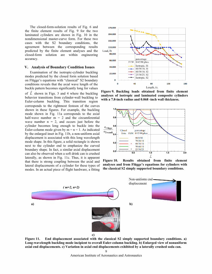
The closed-form-solution results of Fig. 6 and the finite element results of Fig. 9 for the two laminated cylinders are shown in Fig. 10 in the nondimensional master-curve form. For these two cases with the S2 boundary conditions, the agreement between the corresponding results predicted by the finite element analyses and the closed-form solution are within engineering accuracy.

V. Analysis of Boundary Condition Issues Examination of the isotropic-cylinder buckling

modes predicted by the closed form solution based on Flügge’s equations with “classical” S2 boundary conditions reveals that the axial wave length of the buckle pattern becomes significantly long for values

of L shown in Figs. 3 and 4 where the buckling behavior transitions from cylinder-wall buckling to Euler-column buckling. This transition region corresponds to the rightmost festoon of the curves shown in these figures. For example, the buckling mode shown in Fig. 11a corresponds to the axial half-wave number m = 2 and the circumferential wave number n = 2, and occurs just before the cylinder becomes long enough to buckle into the Euler-column mode given by m = n = 1. As indicated by the enlarged inset in Fig. 11b, a non-uniform axial displacement is associated with this long wavelength mode shape. In this figure, a solid rectangle is shown next to the cylinder end to emphasize the curved boundary shape. In fact, a similar axial displacement can also be observed when a soft drink can is crushed laterally, as shown in Fig. 11c. Thus, it is apparent that there is strong coupling between the axial and lateral displacements of a cylinder for these types of modes. In an actual piece of flight hardware, a fitting

Figure 10. Results obtained from finite element analyses and from Flügge’s equations for cylinders with the classical S2 simply supported boundary conditions.

a) b)

c) Figure 11. End displacement associated with the classical S2 simply supported boundary conditions. a) Long-wavelength buckling mode incipient to overall Euler-column buckling. b) Enlarged view of nonuniform axial end displacements. c) Variation in axial end displacements exhibited by a laterally crushed soda can.

Figure 9. Buckling loads obtained from finite element analyses of isotropic and laminated composite cylinders with a 7.8-inch radius and 0.068 -inch wall thickness.


10

may be present that provides a significant amount of axial displacement restraint. Thus, an effort was undertaken in the present study to assess the importance of axial restraint on the buckling response of the isotropic and orthotropic cylinders considered herein.

To assess the effects of axial restraint on the buckling response, additional finite element analyses were conducted on the quasi-isotropic laminate with 25% 0-degree plies, 50% ±45-degree plies, and 25% 90-degree plies and on the laminate with 60% 0-degree plies, 30% ±45-degree plies, and 10% 90-degree plies. These finite element analyses are expected to possess the same level of theoretical fidelity as Flügge’s equations. The boundary conditions used for these analyses are also regarded as simply supported ends but fully restrain the axial displacement. The specific form of the boundary conditions, designated as S1 boundary conditions, is u = 0, v = 0, w = 0, and Mxx = 0. This particular set of boundary conditions requires that all points on the end of the cylinder remain coplanar during buckling.

The finite element results for the S1 boundary conditions are also shown in Fig. 9. In particular, the gold symbols correspond to results for isotropic cylinders and the blue symbols corresponds to results for the laminated cylinders with 60% 0-degree plies, 30% ±45-degree plies, and 10% 90-degree plies. The rightmost descending branch of these two curves also corresponds to Euler-column buckling modes.

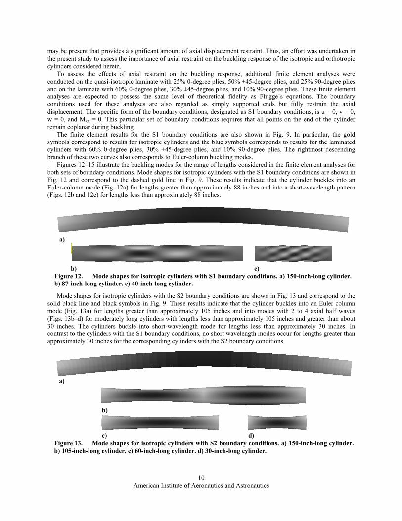
Figures 12–15 illustrate the buckling modes for the range of lengths considered in the finite element analyses for both sets of boundary conditions. Mode shapes for isotropic cylinders with the S1 boundary conditions are shown in Fig. 12 and correspond to the dashed gold line in Fig. 9. These results indicate that the cylinder buckles into an Euler-column mode (Fig. 12a) for lengths greater than approximately 88 inches and into a short-wavelength pattern (Figs. 12b and 12c) for lengths less than approximately 88 inches.

Mode shapes for isotropic cylinders with the S2 boundary conditions are shown in Fig. 13 and correspond to the solid black line and black symbols in Fig. 9. These results indicate that the cylinder buckles into an Euler-column mode (Fig. 13a) for lengths greater than approximately 105 inches and into modes with 2 to 4 axial half waves (Figs. 13b–d) for moderately long cylinders with lengths less than approximately 105 inches and greater than about 30 inches. The cylinders buckle into short-wavelength mode for lengths less than approximately 30 inches. In contrast to the cylinders with the S1 boundary conditions, no short wavelength modes occur for lengths greater than approximately 30 inches for the corresponding cylinders with the S2 boundary conditions.

a)

b) c) Figure 12. Mode shapes for isotropic cylinders with S1 boundary conditions. a) 150-inch-long cylinder. b) 87-inch-long cylinder. c) 40-inch-long cylinder.

a)

b)

c) d) Figure 13. Mode shapes for isotropic cylinders with S2 boundary conditions. a) 150-inch-long cylinder. b) 105-inch-long cylinder. c) 60-inch-long cylinder. d) 30-inch-long cylinder.


11

Buckling modes for the laminated-composite cylinders with 60% 0-degree plies, 30% ±45-degree plies, and 10% 90-degree plies and with the S1 boundary conditions are shown in Fig. 14, and correspond to the blue dashed line shown in Fig. 9. These cylinders buckle into an Euler-column mode (Fig. 14a) for lengths greater than approximately 125 inches and into short-wavelength modes for the smaller lengths (Figs. 14b and 14c).

Buckling modes for the laminated-composite cylinders with 60% 0-degree plies, 30% ±45-degree plies, and 10% 90-degree plies and with the S2 boundary conditions are shown in Fig. 15, and correspond to the purple curve shown in Fig. 9. These cylinder buckles into an Euler-column mode (Fig. 15a) for lengths greater than approximately 145 inches and into modes with 2 to 4 axial half waves (Figs. 15b and 15c) for moderately long cylinders with lengths less than approximately 145 inches and greater than about 40 inches. Cylinders with lengths less than about 40 inches buckle into short-wavelength modes like that shown in Fig. 15d.

To obtain a somewhat generic picture of the boundary condition effects, the results for the “classical” S2 boundary conditions and the axially restrained S1 boundary conditions are shown in master-curve form in Fig. 16 for the isotropic cylinders and in Fig. 17 for the laminated cylinders with walls comprised of 60% 0-degree plies, 30% ±45-degree plies, and 10% 90-degree

a)

b)

c) Figure 14. Mode shapes for laminated cylinders with 60% 0-degree plies, 30% ±45-degree plies, 10% 90-degree plies, and with the S1 boundary conditions. a) 150-inch-long cylinder. b) 120-inch-long cylinder. c) 40-inch-long cylinder.

a)

b)

c) d) Figure 15. Mode shapes for laminated cylinder with 60% 0-degree plies, 30% ±45-degree plies, 10% 90-degree plies, and with the S2 boundary conditions. a) 150-inch-long cylinder. b) 140-inch-long cylinder. c) 87-inch-long cylinder. d) 40-inch-long cylinder.

Figure 16. Effects of boundary conditions on the buckling of isotropic cylinders (ν = 0.3).


12

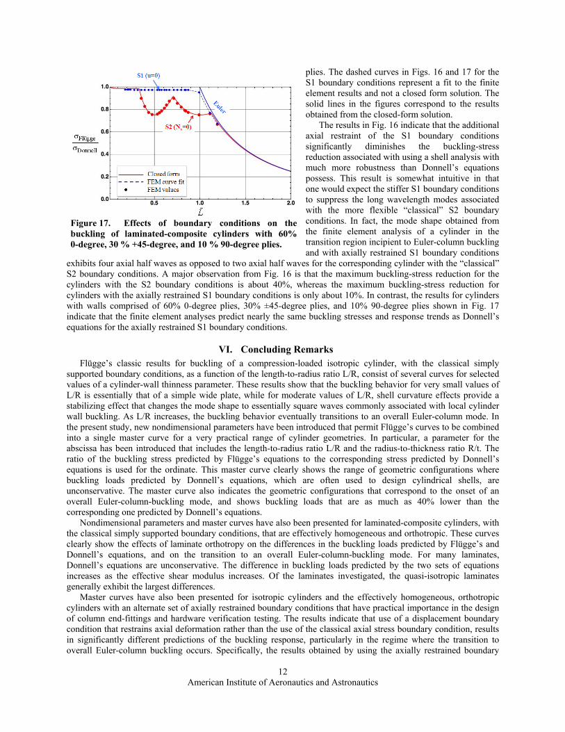
plies. The dashed curves in Figs. 16 and 17 for the S1 boundary conditions represent a fit to the finite element results and not a closed form solution. The solid lines in the figures correspond to the results obtained from the closed-form solution.

The results in Fig. 16 indicate that the additional axial restraint of the S1 boundary conditions significantly diminishes the buckling-stress reduction associated with using a shell analysis with much more robustness than Donnell’s equations possess. This result is somewhat intuitive in that one would expect the stiffer S1 boundary conditions to suppress the long wavelength modes associated with the more flexible “classical” S2 boundary conditions. In fact, the mode shape obtained from the finite element analysis of a cylinder in the transition region incipient to Euler-column buckling and with axially restrained S1 boundary conditions

exhibits four axial half waves as opposed to two axial half waves for the corresponding cylinder with the “classical” S2 boundary conditions. A major observation from Fig. 16 is that the maximum buckling-stress reduction for the cylinders with the S2 boundary conditions is about 40%, whereas the maximum buckling-stress reduction for cylinders with the axially restrained S1 boundary conditions is only about 10%. In contrast, the results for cylinders with walls comprised of 60% 0-degree plies, 30% ±45-degree plies, and 10% 90-degree plies shown in Fig. 17 indicate that the finite element analyses predict nearly the same buckling stresses and response trends as Donnell’s equations for the axially restrained S1 boundary conditions.

VI. Concluding Remarks Flügge’s classic results for buckling of a compression-loaded isotropic cylinder, with the classical simply

supported boundary conditions, as a function of the length-to-radius ratio L/R, consist of several curves for selected values of a cylinder-wall thinness parameter. These results show that the buckling behavior for very small values of L/R is essentially that of a simple wide plate, while for moderate values of L/R, shell curvature effects provide a stabilizing effect that changes the mode shape to essentially square waves commonly associated with local cylinder wall buckling. As L/R increases, the buckling behavior eventually transitions to an overall Euler-column mode. In the present study, new nondimensional parameters have been introduced that permit Flügge’s curves to be combined into a single master curve for a very practical range of cylinder geometries. In particular, a parameter for the abscissa has been introduced that includes the length-to-radius ratio L/R and the radius-to-thickness ratio R/t. The ratio of the buckling stress predicted by Flügge’s equations to the corresponding stress predicted by Donnell’s equations is used for the ordinate. This master curve clearly shows the range of geometric configurations where buckling loads predicted by Donnell’s equations, which are often used to design cylindrical shells, are unconservative. The master curve also indicates the geometric configurations that correspond to the onset of an overall Euler-column-buckling mode, and shows buckling loads that are as much as 40% lower than the corresponding one predicted by Donnell’s equations.

Nondimensional parameters and master curves have also been presented for laminated-composite cylinders, with the classical simply supported boundary conditions, that are effectively homogeneous and orthotropic. These curves clearly show the effects of laminate orthotropy on the differences in the buckling loads predicted by Flügge’s and Donnell’s equations, and on the transition to an overall Euler-column-buckling mode. For many laminates, Donnell’s equations are unconservative. The difference in buckling loads predicted by the two sets of equations increases as the effective shear modulus increases. Of the laminates investigated, the quasi-isotropic laminates generally exhibit the largest differences.

Master curves have also been presented for isotropic cylinders and the effectively homogeneous, orthotropic cylinders with an alternate set of axially restrained boundary conditions that have practical importance in the design of column end-fittings and hardware verification testing. The results indicate that use of a displacement boundary condition that restrains axial deformation rather than the use of the classical axial stress boundary condition, results in significantly different predictions of the buckling response, particularly in the regime where the transition to overall Euler-column buckling occurs. Specifically, the results obtained by using the axially restrained boundary

Figure 17. Effects of boundary conditions on the buckling of laminated-composite cylinders with 60% 0-degree, 30 % +45-degree, and 10 % 90-degree plies.


13

condition predict a much more benign reduction in buckling load with increasing length-to-radius ratio. For an isotropic cylinder, the maximum buckling-stress reduction for the axially restrained boundary condition is only about 10% as compared to the 40% reduction obtained by using the classical axial stress boundary condition. For the laminate-composite cylinders with axially restrained boundaries analyzed in the present study, festoon response curves were not obtained and the buckling loads predicted are nearly the same as the corresponding ones predicted by Donnell’s equations. These results clearly show that considerable care should be taken when selecting boundary conditions for a specific application and laminate configuration.

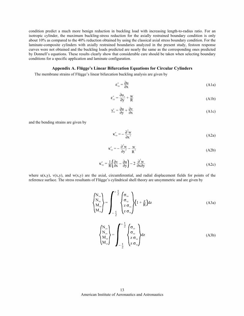
Appendix A. Flügge’s Linear Bifurcation Equations for Circular Cylinders The membrane strains of Flügge’s linear bifurcation buckling analysis are given by

εxx

o = ∂u∂x

(A1a)

εyy

o =∂uy

∂y + wR

(A1b)

γxy

o = ∂u∂y + ∂v

∂x (A1c)

and the bending strains are given by

κ xx

o= − ∂2

w∂x2

(A2a)

κ yy

o= − ∂ 2

w∂y2 − w

R2

(A2b)

κ xy

o= 1

R∂v∂x − ∂u

∂y − 2 ∂2w

∂x∂y (A2c)

where u(x,y), v(x,y), and w(x,y) are the axial, circumferential, and radial displacement fields for points of the reference surface. The stress resultants of Flügge’s cylindrical shell theory are unsymmetric and are given by

Nxx

Nxy

Mxx

Mxy

=

σxx

σxy

z σxx

z σxy

1 + zR

dz

− t2

+ t2

(A3a)

Nyy

Nyx

Myy

Myx

=

σyy

σxy

z σxx

z σxy

dz

− t2

+ t2

(A3b)


14

where σxx, σyy, and σxy are the stresses acting in the shell wall, and t is the wall thickness. The constitutive equations are given by

Nxx

Nyy

Nxy

Nyx

=

A 11 +B11

RA 12 +

B12

RA 16 +

B16

R+

D16

2R2

A 12 A 22 A 26 +D26

2R2

A 16 +B16

RA 26 +

B26

RA 66 +

B66

R+

D66

2R2

A 16 A 26 A 66 +D66

2R2

εxx

o

εyy

o

γxy

o+

B11 +D11

RB12 B16 +

D16

2R

B12 B22 –D22

RB26 –

D26

2R

B16 +D16

RB26 B66 +

D66

2R

B16 B26 –D26

RB66 –

D66

2R

κ xx

o

κ yy

o

κ xy

o

(A4a)

Mxx

Myy

Mxy

Myx

=

B11 +D11

RB12 B16 +

D16

2R

B12 B22 –D22

RB26 –

D26

2R

B16 +D16

RB26 B66 +

D66

2R

B16 B26 –D26

RB66 –

D66

2R

εxx

o

εyy

o

γxy

o+

D11 D12 D16

D12 D22 D26

D16 D26 D66

D16 D26 D66

κ xx

o

κ yy

o

κ xy

o

(A4b)

where the subscripted A, B, and D terms are identical to those given by Jones4 for plates. The equilibrium equations are given by

∂Nxx

∂x +∂Nyx

∂y + Nxx

(0) ∂2u

∂x2 + Nyy

(0) ∂2u

∂y2 − 1R

∂w∂x + 2Nxy

(0) ∂2u

∂x∂y = 0 (A5a)

∂Nxy

∂x +∂Nyy

∂y +1R

∂Mxy

∂x +∂Myy

∂y + Nxx

(0) ∂2v

∂x2

+ Nyy

(0) ∂2v

∂y2 + 1R

∂w∂y + 2Nxy

(0) ∂2v

∂x∂y + 1R

∂w∂x = 0 (A5b)

∂2Mxx

∂x2 +∂2

Myx

∂x∂y +∂2

Mxy

∂x∂y +∂2

Myy

∂y2 –Nyy

R+ Nxx

(0) ∂2w

∂x2

+ Nyy

(0) 1R

∂u∂x − 1

R∂v∂y + ∂2

w∂y2 + 2Nxy

(0) ∂2w

∂x∂y − 1R

∂v∂x = 0 . (A5c)

Similarly, the boundary conditions at x = 0 and x = L are given by

Nxx + N xx

(0) ∂u∂x + Nxy

(0) ∂u∂y = 0 or u = 0 (A6a)

Nxy +

Mxy

R+ Nxx

(0) ∂v∂x + Nxy

(0) ∂v∂y +

wR = 0 or v = 0 (A6b)

∂Mxx

∂x +∂

∂y Mxy + Myx + Nxx

(0) ∂w∂x + Nxy

(0) ∂w∂y −

vR

= 0 or w = 0. (A6c)

Mxx = 0 or ∂w

∂x = 0. (A6d)


15

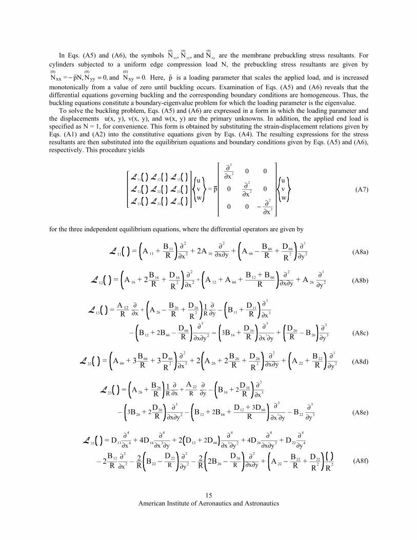
In Eqs. (A5) and (A6), the symbols Nxx

(0)

, Nyy

(0)

, and Nxy

(0)

are the membrane prebuckling stress resultants. For cylinders subjected to a uniform edge compression load N, the prebuckling stress resultants are given by (0) (0)

xx yyN = pN, N 0,− = and (0)

xyN 0.= Here, p is a loading parameter that scales the applied load, and is increased

monotonically from a value of zero until buckling occurs. Examination of Eqs. (A5) and (A6) reveals that the differential equations governing buckling and the corresponding boundary conditions are homogeneous. Thus, the buckling equations constitute a boundary-eigenvalue problem for which the loading parameter is the eigenvalue.

To solve the buckling problem, Eqs. (A5) and (A6) are expressed in a form in which the loading parameter and the displacements u(x, y), v(x, y), and w(x, y) are the primary unknowns. In addition, the applied end load is specified as N = 1, for convenience. This form is obtained by substituting the strain-displacement relations given by Eqs. (A1) and (A2) into the constitutive equations given by Eqs. (A4). The resulting expressions for the stress resultants are then substituted into the equilibrium equations and boundary conditions given by Eqs. (A5) and (A6), respectively. This procedure yields

L 11 L 12 L 13

L 12 L 22 L 23

L 13 L 23 L 33

uvw

= p

∂2

∂x2 0 0

0 ∂2

∂x2 0

0 0 − ∂2

∂x2

uvw

(A7)

for the three independent equilibrium equations, where the differential operators are given by

L 11 = A 11 +

B11

R∂ 2

∂x2 + 2A 16

∂2

∂x∂y + A 66 –B66

R +D66

R2

∂2

∂y2 (A8a)

L 12 = A 16 + 2

B16

R +D16

R2

∂2

∂x2 + A 12 + A 66 +B12 + B66

R∂ 2

∂x∂y + A 26

∂2

∂y2 (A8b)

L 13 =A 12

R∂∂x + A 26 –

B26

R +D26

R2

1R

∂∂y – B11 +

D11

R∂3

∂x3

– B12 + 2B66 –D66

R∂3

∂x∂y2 − 3B16 +D16

R∂3

∂x2

∂y+

D26

R – B26

∂3

∂y3 (A8c)

L 22 = A 66 + 3

B66

R + 3D66

R2

∂ 2

∂x2 + 2 A 26 + 2B26

R +D26

R2

∂ 2

∂x∂y + A 22 +B22

R∂2

∂y2 (A8d)

L 23 = A 26 +B26

R1R

∂∂x +

A 22

R∂∂y – B16 + 2

D16

R∂3

∂x3

– 3B26 + 2D26

R∂3

∂x∂y2 – B12 + 2B66 +D12 + 3D66

R

∂3

∂x2

∂y– B22

∂3

∂y3 (A8e)

L 33 = D11

∂4

∂x4 + 4D16

∂4

∂x3∂y+ 2 D12 + 2D66

∂4

∂x2∂y2 + 4D26

∂4

∂x∂y3 + D22

∂4

∂y4

– 2B12

R∂2

∂x2 – 2R B22 −

D22

R∂2

∂y2 – 2R 2B26 −

D26

R∂2

∂x∂y + A 22 − B22

R +D22

R2

R2

(A8f)


16

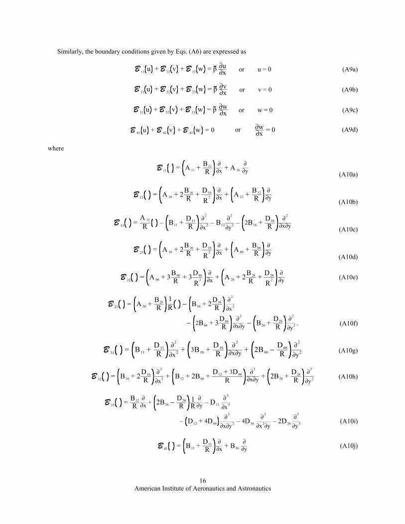
Similarly, the boundary conditions given by Eqs. (A6) are expressed as

B 11 u + B 12 v + B 13 w = p ∂u

∂x or u = 0 (A9a)

B 21 u + B 22 v + B 23 w = p ∂v

∂x or v = 0 (A9b)

B 31 u + B 32 v + B 33 w = p ∂w

∂x or w = 0 (A9c)

B 41 u + B 42 v + B 43 w = 0 or ∂w∂x = 0 (A9d)

where

B 11 = A 11 +

B11

R∂∂x + A 16

∂∂y

(A10a)

B 12 = A 16 + 2

B16

R+

D16

R2

∂∂x + A 12 +

B12

R∂

∂y (A10b)

B 13 =

A 12

R – B11 +D11

R∂2

∂x2 – B12

∂2

∂y2 – 2B16 +D16

R∂2

∂x∂y (A10c)

B 21 = A 16 + 2

B16

R+

D16

R2

∂∂x + A 66 +

B66

R∂

∂y (A10d)

B 22 = A 66 + 3

B66

R + 3D66

R2

∂∂x + A 26 + 2

B26

R +D26

R2

∂∂y (A10e)

B 23 = A 26 +B26

R1R − B16 + 2

D16

R∂2

∂x2

− 2B66 + 3D66

R∂2

∂x∂y − B26 +D26

R∂2

∂y2 . (A10f)

B 31 = B11 +

D11

R∂ 2

∂x2 + 3B16 +D16

R∂ 2

∂x∂y + 2B66 − D66

R∂ 2

∂y2 (A10g)

B 32 = B16 + 2

D16

R∂2

∂x2 + B12 + 2B66 +D12 + 3D66

R∂2

∂x∂y + 2B26 +D26

R∂2

∂y2 (A10h)

B 33 =B12

R∂

∂x + 2B26 − D26

R1R

∂∂y – D11

∂3

∂x3

– D12 + 4D66

∂3

∂x∂y2 – 4D16

∂3

∂x2∂y– 2D26

∂3

∂y3 (A10i)

B 41 = B11 +

D11

R∂

∂x + B16

∂∂y (A10j)


17

B 42 = B16 + 2

D16

R∂

∂x + B12 +D12

R∂

∂y (A10k)

B 43 =

B12

R– D11

∂2

∂x2 – D12

∂2

∂y2 – 2D16

∂2

∂x∂y . (A10l)

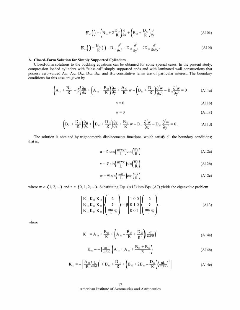
A. Closed-Form Solution for Simply Supported Cylinders Closed-form solutions to the buckling equations can be obtained for some special cases. In the present study,

compression loaded cylinders with "classical" simply supported ends and with laminated wall constructions that possess zero-valued A16, A26, D16, D26, B16, and B26 constitutive terms are of particular interest. The boundary conditions for this case are given by

A 11 +

B11

R − p ∂u∂x + A 12 +

B12

R∂v∂y +

A 12

R w – B11 +D11

R∂2

w∂x2 – B12

∂2w

∂y2 = 0 (A11a)

v = 0 (A11b)

w = 0 (A11c)

B11 +

D11

R∂u∂x + B12 +

D12

R∂v∂y +

B12

R w – D11∂ 2

w∂x2 – D12

∂ 2w

∂y2 = 0. (A11d)

The solution is obtained by trigonometric displacements functions, which satisfy all the boundary conditions; that is,

u = u cos mπx

Lcos

nyR

(A12a)

v = v sin mπx

L sinnyR

(A12b)

w = w sin mπx

L cosnyR

(A12c)

where m ∈ 1, 2, ... and n ∈ 0, 1, 2, ... . Substituting Eqs. (A12) into Eqs. (A7) yields the eigenvalue problem

K11 K12 K13

K12 K22 K23

K13 K23 K33

u

vmπL w

= p

1 0 0

0 1 0

0 0 1

u

vmπL w

. (A13)

where

K11 = A 11 +

B11

R+ A 66 –

B66

R+

D66

R2

nLmπR

2

(A14a)

K12 = – nL

mπR A 12 + A 66 +B12 + B66

R (A14b)

K13 = –

A 12

RL

mπ2

+ B11 +D11

R + B12 + 2B66 –D66

RnL

mπR

2

(A14c)


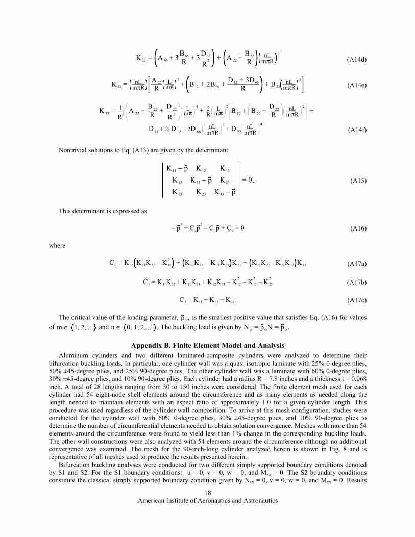
18

K22 = A 66 + 3

B66

R+ 3

D66

R2 + A 22 +

B22

RnL

mπR

2

(A14d)

K23 = nL

mπRA 22

RL

mπ2

+ B12 + 2B66 +D12 + 3D66

R+ B22

nLmπR

2

(A14e)

(A14f)

Nontrivial solutions to Eq. (A13) are given by the determinant

K11 − p K12 K13

K12 K22 − p K23

K13 K23 K33 − p

= 0. (A15)

This determinant is expressed as

− p3

+ C2p2

− C1p + C0 = 0 (A16)

where

C0 = K 33 K 11K 22 – K 12

2+ K12K 13 – K11K 23 K 23 + K 12K 23– K22K 13 K 13 (A17a)

C1 = K11K22 + K11K33 + K22K33 – K12

2– K13

2– K23

2

(A17b)

C2 = K11 + K22 + K33. (A17c)

The critical value of the loading parameter, pcr, is the smallest positive value that satisfies Eq. (A16) for values

of m ∈ 1, 2, ... and n ∈ 0, 1, 2, ... . The buckling load is given by N cr = pcrN = pcr.

Appendix B. Finite Element Model and Analysis Aluminum cylinders and two different laminated-composite cylinders were analyzed to determine their

bifurcation buckling loads. In particular, one cylinder wall was a quasi-isotropic laminate with 25% 0-degree plies, 50% ±45-degree plies, and 25% 90-degree plies. The other cylinder wall was a laminate with 60% 0-degree plies, 30% ±45-degree plies, and 10% 90-degree plies. Each cylinder had a radius R = 7.8 inches and a thickness t = 0.068 inch. A total of 28 lengths ranging from 30 to 150 inches were considered. The finite element mesh used for each cylinder had 54 eight-node shell elements around the circumference and as many elements as needed along the length needed to maintain elements with an aspect ratio of approximately 1.0 for a given cylinder length. This procedure was used regardless of the cylinder wall composition. To arrive at this mesh configuration, studies were conducted for the cylinder wall with 60% 0-degree plies, 30% ±45-degree plies, and 10% 90-degree plies to determine the number of circumferential elements needed to obtain solution convergence. Meshes with more than 54 elements around the circumference were found to yield less than 1% change in the corresponding buckling loads. The other wall constructions were also analyzed with 54 elements around the circumference although no additional convergence was examined. The mesh for the 90-inch-long cylinder analyzed herein is shown in Fig. 8 and is representative of all meshes used to produce the results presented herein.

Bifurcation buckling analyses were conducted for two different simply supported boundary conditions denoted by S1 and S2. For the S1 boundary conditions: u = 0, v = 0, w = 0, and Mxx = 0. The S2 boundary conditions constitute the classical simply supported boundary condition given by Nxx = 0, v = 0, w = 0, and Mxx = 0. Results

K 33 =1 R 2

A 22 −B 22 R

+D 22

R2

Lmπ

4+ 2

RL

mπ2

B 12 + B 22− D 22

RnL

mπR 2

+

D 11 + 2 D 12 + 2D 66nL

mπR

2+ D 22

nLmπR

4


19

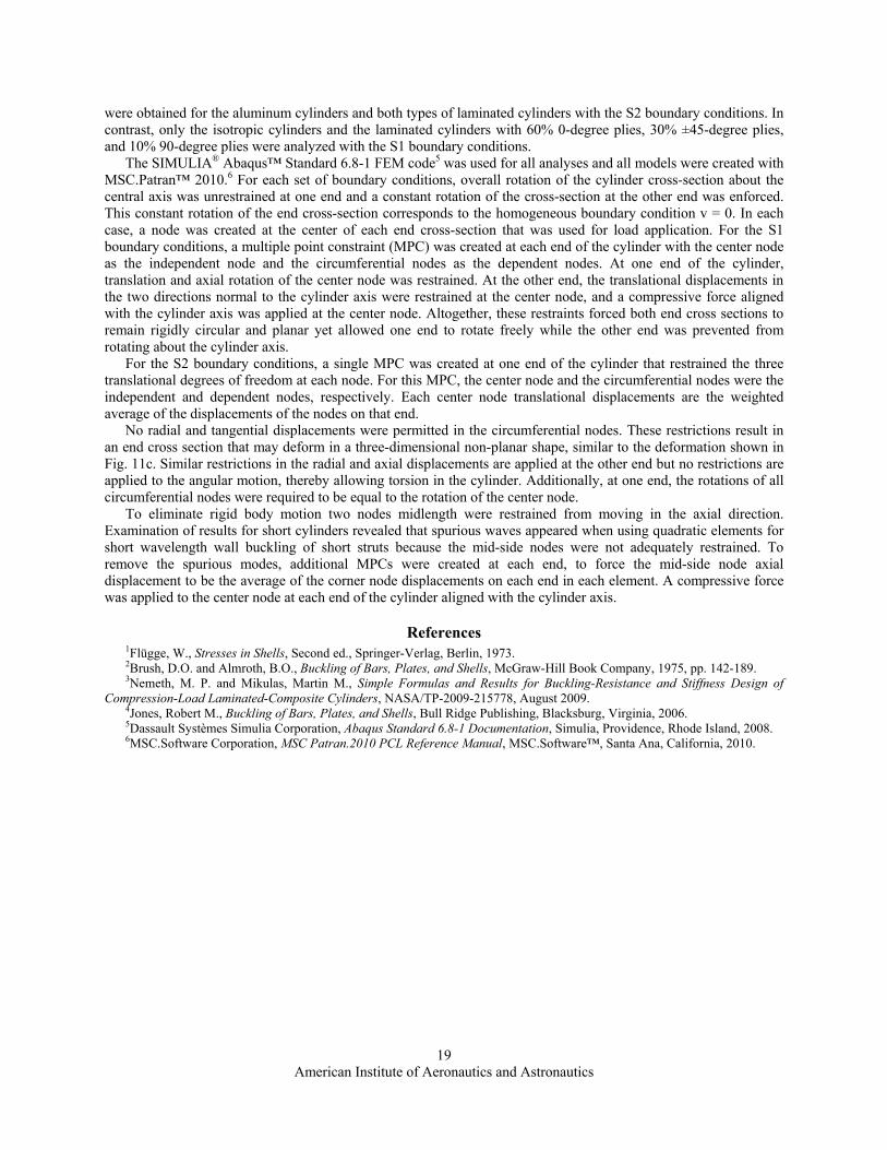
were obtained for the aluminum cylinders and both types of laminated cylinders with the S2 boundary conditions. In contrast, only the isotropic cylinders and the laminated cylinders with 60% 0-degree plies, 30% ±45-degree plies, and 10% 90-degree plies were analyzed with the S1 boundary conditions.

The SIMULIA® Abaqus™ Standard 6.8-1 FEM code5 was used for all analyses and all models were created with MSC.Patran™ 2010.6 For each set of boundary conditions, overall rotation of the cylinder cross-section about the central axis was unrestrained at one end and a constant rotation of the cross-section at the other end was enforced. This constant rotation of the end cross-section corresponds to the homogeneous boundary condition v = 0. In each case, a node was created at the center of each end cross-section that was used for load application. For the S1 boundary conditions, a multiple point constraint (MPC) was created at each end of the cylinder with the center node as the independent node and the circumferential nodes as the dependent nodes. At one end of the cylinder, translation and axial rotation of the center node was restrained. At the other end, the translational displacements in the two directions normal to the cylinder axis were restrained at the center node, and a compressive force aligned with the cylinder axis was applied at the center node. Altogether, these restraints forced both end cross sections to remain rigidly circular and planar yet allowed one end to rotate freely while the other end was prevented from rotating about the cylinder axis.

For the S2 boundary conditions, a single MPC was created at one end of the cylinder that restrained the three translational degrees of freedom at each node. For this MPC, the center node and the circumferential nodes were the independent and dependent nodes, respectively. Each center node translational displacements are the weighted average of the displacements of the nodes on that end.

No radial and tangential displacements were permitted in the circumferential nodes. These restrictions result in an end cross section that may deform in a three-dimensional non-planar shape, similar to the deformation shown in Fig. 11c. Similar restrictions in the radial and axial displacements are applied at the other end but no restrictions are applied to the angular motion, thereby allowing torsion in the cylinder. Additionally, at one end, the rotations of all circumferential nodes were required to be equal to the rotation of the center node.

To eliminate rigid body motion two nodes midlength were restrained from moving in the axial direction. Examination of results for short cylinders revealed that spurious waves appeared when using quadratic elements for short wavelength wall buckling of short struts because the mid-side nodes were not adequately restrained. To remove the spurious modes, additional MPCs were created at each end, to force the mid-side node axial displacement to be the average of the corner node displacements on each end in each element. A compressive force was applied to the center node at each end of the cylinder aligned with the cylinder axis.

References 1Flügge, W., Stresses in Shells, Second ed., Springer-Verlag, Berlin, 1973. 2Brush, D.O. and Almroth, B.O., Buckling of Bars, Plates, and Shells, McGraw-Hill Book Company, 1975, pp. 142-189. 3Nemeth, M. P. and Mikulas, Martin M., Simple Formulas and Results for Buckling-Resistance and Stiffness Design of

Compression-Load Laminated-Composite Cylinders, NASA/TP-2009-215778, August 2009. 4Jones, Robert M., Buckling of Bars, Plates, and Shells, Bull Ridge Publishing, Blacksburg, Virginia, 2006. 5Dassault Systèmes Simulia Corporation, Abaqus Standard 6.8-1 Documentation, Simulia, Providence, Rhode Island, 2008. 6MSC.Software Corporation, MSC Patran.2010 PCL Reference Manual, MSC.Software™, Santa Ana, California, 2010.

effect of boundary conditions on the axial compression … · · 2013-04-10american institute of...

Documents