Efficiently Answering Reachability Queries on Very LargeDirected Graphs

Ruoming Jin† Yang Xiang†† Department of Computer Science

Kent State University, Kent, OH, USA{jin,yxiang,nruan}@cs.kent.edu

Ning Ruan† Haixun Wang‡‡ IBM T.J. Watson Research

Hawthorne, NY, USAhaixun@us.ibm.com

ABSTRACTEfficiently processing queries against very large graphs isan important research topic largely driven by emerging realworld applications, as diverse as XML databases, GIS, webmining, social network analysis, ontologies, and bioinformat-ics. In particular, graph reachability has attracted a lot ofresearch attention as reachability queries are not only com-mon on graph databases, but they also serve as fundamentaloperations for many other graph queries. The main idea be-hind answering reachability queries in graphs is to build in-dices based on reachability labels. Essentially, each vertex inthe graph is assigned with certain labels such that the reach-ability between any two vertices can be determined by theirlabels. Several approaches have been proposed for buildingthese reachability labels; among them are interval labeling(tree cover) and 2-hop labeling. However, due to the largenumber of vertices in many real world graphs (some graphscan easily contain millions of vertices), the computationalcost and (index) size of the labels using existing methodswould prove too expensive to be practical. In this paper,we introduce a novel graph structure, referred to as path-tree, to help labeling very large graphs. The path-tree coveris a spanning subgraph of G in a tree shape. We demon-strate both analytically and empirically the effectiveness ofour new approaches.

Categories and Subject DescriptorsH.2.8 [Database management]: Database Applications—graph indexing and querying

General TermsPerformance

KeywordsGraph indexing, Reachability queries, Transitive closure,Path-tree cover, Maximal directed spanning tree

Permission to make digital or hard copies of all or part of this work forpersonal or classroom use is granted without fee provided that copies arenot made or distributed for profit or commercial advantage and that copiesbear this notice and the full citation on the first page. To copy otherwise, torepublish, to post on servers or to redistribute to lists, requires prior specificpermission and/or a fee.SIGMOD’08, June 9–12, 2008, Vancouver, BC, Canada.Copyright 2008 ACM 978-1-60558-102-6/08/06 ...$5.00.

1. INTRODUCTIONUbiquitous graph data coupled with advances in graph an-

alyzing techniques are pushing the database community topay more attention to graph databases. Efficiently man-aging and answering queries against very large graphs isbecoming an increasingly important research topic drivenby many emerging real world applications: XML databases,GIS, web mining, social network analysis, ontologies, andbioinformatics, to name a few.

Among them, graph reachability queries have attracted alot of research attention. Given two vertices u and v in adirected graph, a reachability query asks if there is a pathfrom u to v. Graph reachability is one of the most commonqueries in a graph database. In many other applicationswhere graphs are used as the basic data structure (e.g., XMLdata management), it is also one of the fundamental opera-tions. Thus, efficient processing of reachability queries is acritical issue in graph databases.

1.1 ApplicationsReachability queries are very important for many XML

databases. Typical XML documents are tree structures.In such cases, the reachability query simply correspondsto ancestor-descendant search (“//”). However, with thewidespread usage of ID and IDREF attributes, which rep-resent relationships unaccounted for by a strict tree struc-ture, it is sometimes more appropriate to represent the XMLdocuments as directed graphs. Queries on such data ofteninvoke a reachability query. For instance, in bibliographicdata which contains a paper citation network, such as inCiteseer, we may ask if author A is influenced by paperB, which can be represented as a simple path expression//B//A. A typical way of processing this query is to obtain(possibly through some index on elements) elements A andB and then test if author A is reachable from paper B inthe XML graph. Clearly, it is crucial to provide efficientsupport for reachability testing due to its importance forcomplex XML queries.

Querying ontologies is becoming increasingly important asmany large domain ontologies are being constructed. One ofthe most well-known ontologies is the gene ontology (GO) 1.GO can be represented as a directed acyclic graph (DAG)in which nodes are concepts (vocabulary terms) and edgesare relationships (is-a or part-of). It provides a controlledvocabulary of terms to describe a gene product, e.g., proteinsor RNA, in any organism. For instance, we may query if acertain protein is related to a certain biological process or

1http://www.geneontology.org

595

has a certain molecular function. In the simple case, thiscan be transformed into a reachability query on two verticesover the GO DAG. As a protein can directly associate withseveral vertices in the DAG, the entire query process mayactually invoke several reachability queries.

Recent advances in system biology have amassed a largeamount of graph data, e.g., various kinds of biological net-works: gene regulatory, protein-protein interaction, signaltransduction, metabolic, etc. Many databases are beingconstructed to maintain these data. Biology and bioinfor-matics are actually becoming a key driving force for graphdatabases. Here again, reachability is one of the fundamen-tal queries frequently used. For instance, we may ask if onegene is (indirectly) regulated by another gene, or if there isa biological pathway between two proteins. Biological net-works may soon reach sizes that require improvements toexisting reachability query techniques.

1.2 Prior WorkIn order to tell whether a vertex u can reach another ver-

tex v in a directed graph G = (V, E), we can use two “ex-treme” approaches. The first approach traverses the graph(by DFS or BFS), which will take O(n + m) time, wheren = |V | (number of vertices) and m = |E| (number ofedges). This is apparently too slow for large graphs. Theother approach precomputes the transitive closure of G, i.e.,it records the reachability between any pair of vertices in ad-vance. While this approach can answer reachability queriesin O(1) time, the computation of transitive closure has com-plexity of O(mn) [14] and the storage cost is O(n2). Bothare unacceptable for large graphs. Existing research hasbeen trying to find good ways to reduce the precomputationtime and storage cost with reasonable answering time.

A key idea which has been explored in existing research isto utilize simpler graph structures, such as chains or trees,in the original graph to compute and compress the transitiveclosure and/or help with reachability answering.

Chain Decomposition Approach. Chains are the firstsimple graph structure which has been studied in both graphtheory and database literature to improve the efficiency ofthe transitive closure computation [14] and to compress thetransitive closure matrix [11]. The basic idea of chain de-composition is as follows: the DAG is partitioned into sev-eral pair-wise disjoint chains (one vertex appears in one andonly one chain). Each vertex in the graph is assigned a chainnumber and its sequence number in the chain. For any ver-tex v and any chain c, we record at most one vertex u suchthat u is the smallest vertex (in terms of u’s sequence num-ber) on chain c that is reachable from v. To tell if any vertexx reaches any vertex y, we only need to check if x reachesany vertex y′ in y’s chain and y′ has a smaller sequencenumber than y.

Currently, Simon’s algorithm [14], which uses chain de-composition to compute the transitive closure, has worstcase complexity O(k· ered), where k is width (the total num-ber of chains) of the chain decomposition and ered is thenumber of edges in the transitive reduction of the DAG G(the transitive reduction of G is the smallest subgraph ofG which has the same transitive closure as G, ered ≤ e).Jagadish et al. [11] applied chain decomposition to reducethe size of a transitive closure matrix. It finds the minimalnumber of chains from G by transforming the problem to

an equivalent network flow problem, which can be solved inO(n3), where n is the number of vertices in DAG G. Sev-eral heuristic algorithms have been proposed to reduce thecomputational cost for chain decomposition.

Even though chain decomposition can help with compress-ing the transitive closure, its compression rate is limited bythe fact that each node can have no more than one immedi-ate successor. In many applications, even though the graphsare rather sparse, each node can have multiple immediatesuccessors, and the chain decomposition can consider onlyat most one of them.

Tree Cover Approach. Instead of using chains, Agrawalet al. use a (spanning) tree to “cover” the graph and com-press the transitive closure matrix. They show that the treecover can beat the best chain decomposition [1]. The pro-posed algorithm finds the best tree cover that can maximallycompress the transitive closure. The cost of such a pro-cedure, however, is equivalent to computing the transitiveclosure.

The idea of tree cover is based on interval labeling. Givena tree, we assign each vertex a pair of numbers (an interval).If vertex u can reach vertex v, then the interval of u containsthe interval of v. The interval can be obtained by performinga postorder traversal of the tree. Each vertex v is associatedwith an interval (i, j), where j is the postorder number ofvertex v and i is the smallest postorder number among itsdescendants (each vertex is a descendant of itself).

Assume we have found a tree cover (a spanning tree) ofthe given DAG G, and vertices of G are indexed by theirinterval label. Then, for any vertex, we only need to re-member those nodes that it can reach, but the reachabilityis not embodied by the interval labels. Thus, the transi-tive closure can be compressed. In other words, if u reachesthe root of a subtree, then we only need to record the rootvertex as the interval of any other vertex in the subtree iscontained by that of the root vertex. To answer whether ucan reach v, we will check if the interval of v is contained byany interval associated with the vertices we have recordedfor u.

Other Variants of Tree Covers (Dual-Labeling, La-bel+SSPI, and GRIPP). Several recent studies try toaddress the deficiency of the tree cover approach by Agrawalet al. Wang et al. [16] develop the Dual-Labeling approachwhich tries to improve the query time and index size for thesparse graph, as the original tree cover would cost O(n) andO(n2), respectively. For a very sparse graph, they claim thenumber of non-tree edges t is much smaller than n (t << n).Their approaches can reduce the index size to O(n+ t2) andachieve constant query answering time. Their major ideais to build a transitive link matrix, which can be thoughtof as the transitive closure for the non-tree edges. Basi-cally, each non-tree edge is represented as a vertex and apair of them is linked if the starting of one edge v can bereached by the end of another edge u through the intervalindex (v is u’s descendant in the tree cover). They developapproaches to utilize this matrix to answer the reachabilityquery with constant time. In addition, the tree generated indual-labeling is different from the optimal tree cover, as herethe goal is to minimize the number of non-tree edges. Thisis essentially equivalent to the transitive reduction computa-tion which has proved to be as costly as the transitive closure

596

computation. Thus, their approach (including the transitivereduction) requires an additional O(nm) construction timeif non-tree edges should be minimized. Clearly, the majorissue of this approach is that it depends heavily on the num-ber of non-tree edges. If t > n or mred ≥ 2n, this approachwill not help with the computation of transitive closure, orcompress the index size.

Label+SSPI [2] and GRIPP [15] aim to minimize the in-dex construction time and index size. They achieve O(m+n)index construction time and O(m + n) index size. How-ever, this is at the sacrifice of the query time, which willcost O(m − n). Both algorithms start by extracting a treecover. Label+SSPI utilizes pre- and post-order labeling fora spanning tree and an additional data structure for storingnon-tree edges. GRIPP builds the cover using a depth-firstsearch traversal, and each vertex which has multiple incom-ing edges will be duplicated accordingly in the tree cover.In some sense, their non-tree edges are recorded as non-treevertex instances in the tree cover. To answer a query, bothof them will deploy an online search over the index to see ifu can reach v. GRIPP has developed a couple of heuristicswhich utilize the interval property to speed up the searchprocess.

2-HOP Labeling. The 2-hop labeling method proposedby Cohen et al. [5] represents a quite different approach. In-tuitively, it tries to identify a subset of vertices Vs in thegraph which best capture the connectivity information ofthe DAG. Then, for each vertex v in the DAG, we record alist of vertices in Vs which can reach v, denoted as Lin(v),and a list of vertices in Vs which v can reach, denoted asLout(v). These two sets record all the necessary informationto infer the reachability of any pair of vertices u and v, i.e., ifu→ v, then Lout(v)∩Lin(v) �= ∅, and vice versa. For a givenlabeling, the index size is I =

Pv∈V |Lin(v)| + |Lout(v)|.

They propose an approximate (greedy) algorithm based onset-covering which can produce a 2-hop cover with size nolarger than the minimum possible 2-hop cover by a loga-rithmic factor. The minimum 2-hop cover is conjectured tobe O(nm1/2). However, their original algorithm will requirecomputing the transitive closure first with an O(n4) timecomplexity to find the good 2-hop cover.

Recently, several approaches have been proposed to reducethe construction time of 2-hop. Schenkel et al. propose theHOPI algorithm, which applies a divide-and-conquer strat-egy to compute 2-hop labeling [13]. They reduce the 2-hop labeling complexity from O(n4) to O(n3), which is stillvery expensive for large graphs. Cheng et al. [3] proposea geometric-based algorithm to produce a 2-hop labeling.Their algorithm does not require the computation of tran-sitive closure, but it does not produce the approximationbound of the labeling size which is produced by Cohen’sapproach.

1m is the number of edges and O(n3) if using Floyd-Warshallalgorithm [6]2k is the width of chain decomposition; Query time can beimproved to O(log k) (assuming binary search) and construc-tion time becomes O(mn+n2 log n), which includes the costof sorting.3Query time can be improved to O(log n) and constructiontime becomes O(mn + n2 log n).4The index size is still a conjecture.5It requires an additional O(nm) construction time if the

Query time Construction time Index sizeTransitive Closure O(1) O(nm)1 O(n2)Opt. Chain Cover2 O(k) O(nm) O(nk)Opt. Tree Cover 3 O(n) O(nm) O(n2)2-Hop4 O(m1/2) O(n4) O(nm1/2)

HOPI4 O(m1/2) O(n3) O(nm1/2)Dual Labeling5 O(1) O(n + m + t3) O(n + t2)Labeling+SSPI O(m − n) O(n + m) O(n + m)GRIPP O(m − n) O(n + m) O(n + m)

Table 1: Complexity comparison

1.3 Our ContributionIn Table 1 we show the indexing and querying complexity

of different reachability approaches. Throughout the abovecomparison and several existing studies [15, 16, 13], we cansee that even though the 2-hop approach is theoretically ap-pealing, it is rather difficult to apply it on very large graphsdue to its computational cost. At the same time, as mostof the large graph is rather sparse, the tree-based approachseems to provide a good starting point to compress transi-tive closure and to answer reachability queries. Most of therecent studies try to improve different aspects of the tree-based approach [1, 16, 2, 15]. Since we can effectively trans-form any directed graph into a DAG by contracting stronglyconnected components into vertices and utilizing the DAGto answer the reachability query, we will only focus on DAGfor the rest of the paper.

Our study is motivated by a list of challenging issues whichtree-based approaches do not adequately address. First ofall, the computational cost of finding a good tree cover canbe expensive. For instance, it costs O(mn) to extract atree cover with Agrawal’s optimal tree cover [1] and Wang’sDual-labeling tree [16]. Second, the tree cover cannot rep-resent some common types of DAGs, for instance, the Gridtype of DAG [13], where each vertex in the graph links to itsright and upper corners. For a k×k grid, the tree cover canmaximally cover half of the edges and the compressed tran-sitive closure is almost as big as the original one. We believethe difficulty here is that the strict tree structures are toolimited to express many different types of DAGs even whenthey are very sparse. From another perspective, most ofthe existing methods which utilize the tree cover are greatlyaffected by how many edges are left uncovered.

Driven by these challenges, in this paper, we propose anovel graph structure, referred to as path-tree, to cover aDAG. It creates a tree structure where each node in thetree represents a path in the original graph. This poten-tially doubles our capability to cover DAGs. Given thatmany real world graphs are very sparse, e.g., the numberof edges is no more than 2 times of the number of vertices,the path-tree provides us a better tool to cover the DAG.In addition, we develop a labeling scheme where each labelhas only 3 elements in the path-tree to answer a reacha-bility query. We show that a good path-tree cover can beconstructed in O(m + n log n) time. Theoretically, we provethat the path-tree cover can always perform the compres-sion of transitive closure better than or equal to the optimaltree cover approaches and chain decomposition approaches.Finally, we note that our approach can be combined withexisting methods to handle non-path-tree edges. We have

number of non-tree edges should be minimized.

597

performed a detailed experimental evaluation on both realand synthetic datasets. Our results show that the path-treecover can significantly reduce the transitive closure size andimprove query answering time.

The rest of the paper is organized as follows. In Section 2,we introduce the path-tree concept and an algorithm to con-struct a path-tree from the DAG. In Section 3, we investigateseveral optimality questions related to path-tree cover. InSection 4, we present the experimental results. We concludein Section 5.

2. PATH-TREE COVER FOR REACHABIL-ITY QUERY

We propose to use a novel graph structure, Path-Tree, tocover a DAG G. The path-tree cover is a spanning subgraphof G in a tree shape. Under a labeling scheme we devise forthe path-tree cover wherein each vertex is labeled with a 3-tuple, we can answer reachability queries in O(1) time. Wealso show that a good path-tree cover can be extracted fromG to help reduce the size of G’s transitive closure.

Below, Section 2.1 defines notations used in this paper.Section 2.2 describes how to partition a DAG into paths.Using this partitioning, we define the path-pair subgraph ofG and reveal a nice structure of this subgraph (Section 2.3).We then discuss how to extract a good path-tree cover fromG (Section 2.4). We present the labeling schema for thepath-tree cover in Section 2.5. Finally, we show how thepath-tree cover can be applied to compress the transitiveclosure of G in Section 2.6.

2.1 NotationsLet G = (V, E) be a directed acyclic graph (DAG), where

V = {1, 2, · · · , n} is the vertex set, and E ⊆ V × V is theedge set. We use (v, w) to denote the edge from vertex v tovertex w, and we use (v0, v1, · · · , vp) to denote a path fromvertex v0 to vertex vp, where (vi, vi+1) is an edge (0 ≤ i ≤p − 1). Because G is acyclic, all vertices in a path must bepairwise distinct. We say vertex v is reachable from vertexu (denoted as u→ v) if there is a path starting from u andending at v.

For a vertex v, we refer to all edges that start from v asoutgoing edges of v, and all edges ending at v as incomingedges of v. The predecessor set of vertex v, denoted as S(v),is the set of all vertices that can reach v, and the successorset of vertex v, denoted as R(v), is the set of all verticesthat v can reach. The successor set of v is also called thetransitive closure of v. The transitive closure of DAG G isthe directed graph where there is a direct edge from eachvertex v to any vertex in its successor set.

In addition, we say Gs = (Vs, Es) is a subgraph of G =(V, E) if Vs ⊆ V and Es ⊆ E∩ (Vs×Vs). We denote Gs as aspanning subgraph of G if it covers all the vertices of G, i.e.,Vs = V . A tree T is a special DAG where each vertex hasonly one incoming edge (except for the root vertex, whichdoes not have any incoming edge). A forest (or branching)is a union of multiple trees. A forest can be converted intoa tree by simply adding a virtual vertex with an edge to theroots of each individual tree. To simplify our discussion, wewill use trees to refer to both trees and forests.

In this paper, we introduce a novel graph structure calledpath-tree cover (or simply path-tree). A path-tree cover forG, denoted as G[T ] = (V, E′, T ), is a spanning subgraph

(a) (b)

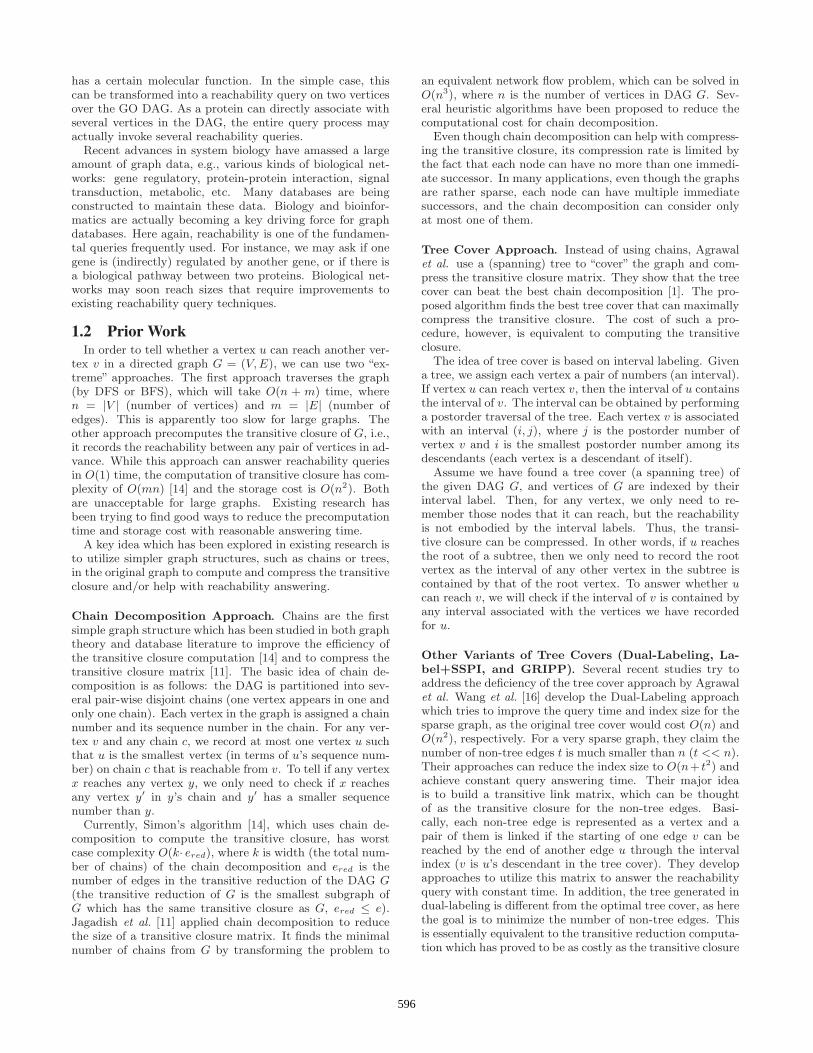
Figure 1: Path-Decomposition for a DAG

of G and has a tree-like shape which is described by treeT = (VT , ET ): Each vertex v of G is uniquely mapped toa single vertex in T , denoted as f(v) ∈ VT , and each edge(u, v) in E′ is uniquely mapped to either a single edge in T ,(f(u), f(v)) ∈ ET , or a single vertex in T .

2.2 Path-Decomposition of DAGLet P1, P2 be two paths of G. We use P1 ∩ P2 to denote

the set of vertices that appear in both paths, and we useP1 ∪ P2 to denote the set of vertices that appear in at leastone of the two paths. We define graph partitions based onthe above terminology.

Definition 1. Let G = (V, E) be a DAG. We say a par-tition P1, · · · , Pk of V is a path-decomposition of G if andonly if P1 ∪ · · · ∪ Pk = V , and Pi ∩ Pj = ∅ for any i �= j.We also refer to k as the width of the decomposition.

As an example, Figure 1(b) represents a partition of graphG in Figure 1(a). The path decomposition contains fourpaths P1 = {1, 3, 6, 13, 14, 15}, P2 = {2, 4, 7, 10, 11}, P3 ={5, 8} and P4 = {9, 12}.

Based on the partition, we can identify each vertex v by apair of IDs: (pid, sid), where pid is the ID of the path vertexv belongs to, and sid is v’s relative order on that path. Forinstance, vertex 3 in G shown in Figure 1(b) is identified by(1, 2). For two vertices u and v in path Pi, we use u � v todenote u precedes v (or u = v) in path Pi:

u � v ⇐⇒ u.sid ≤ v.sid and u, v ∈ Pi

NOTE: A simple path-decomposition algorithm is givenby [14]. It can be described briefly as follows: first, we per-form a topological sort of the DAG. Then, we extract pathsfrom the DAG as follows. We find v, the smallest vertex(in the ascending order of the topological sort) in the graphand add it to the path. We then find v′, such that v′ isthe smallest vertex in the graph such that there is an edgefrom v to v′. In other words, we repeatedly add the smallestnodes to the latest extracted vertex until the path could notbe extended (the vertex added last has no out-going edges).Then, we remove the entire path (including the edges con-necting to it) from the DAG and extract another path. Thedecomposition is complete when the DAG is empty.

2.3 Path Subgraph and Minimal EquivalentEdge Set

Let us consider the relationships between two paths. Weuse Pi → Pj to denote the subgraph of G consisting of i) path

598

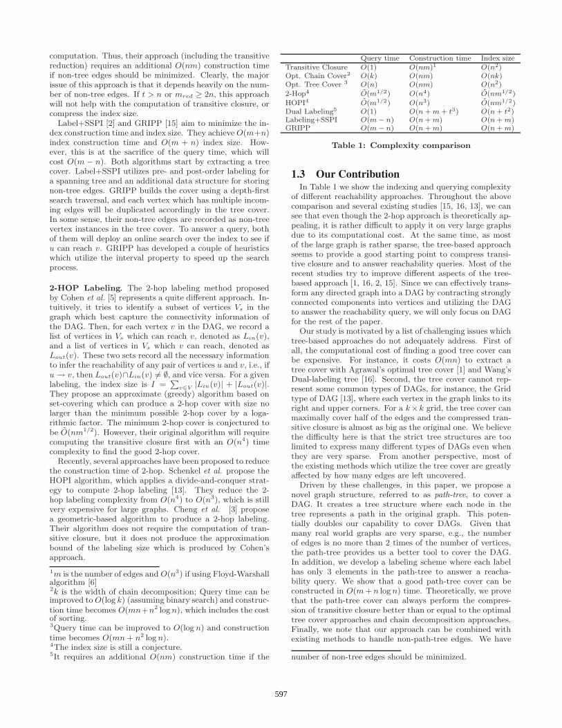
Pi, ii) path Pj , and iii) EPi→Pj , which is the set of edgesfrom vertices on path Pi to vertices on path Pj . For instance,EP1→P2 = {(1, 4), (1, 7), (3, 4), (3, 7), (13, 11)} is the set ofedges from vertices in P1 to vertices in P2. We say subgraphPi → Pj is connected if EPi→Pj is not empty.

Given a vertex u in path Pi, we want to find all verticesin path Pj that are reachable from u (through paths in sub-graph Pi → Pj only). It turns out that we only need toknow one vertex – the smallest (with regard to sequence id)vertex on path Pj reachable from u. We denote its sid asrj(u).

rj(u) = min{v.sid|u→ v and v.pid = j}Clearly, for any vertex v′ ∈ Pj ,

u→ v′ ⇐⇒ v′.sid ≥ rj(u)

Certain edges in EPi→Pj can be removed without changingthe reachability between any two vertices in subgraph Pi →Pj . This is characterized by the following definition.

Definition 2. A set of edges ERPi→Pj

⊆ EPi→Pj is calledthe minimal equivalent edge set of EPi→Pj if removing any

edge from ERPi→Pj

changes the reachability of vertices inPi → Pj .

As shown in Figure 2(a), {(3, 4), (13, 11)} is the minimalequivalent edge set for subgraph P1 → P2. In Figure 2(b),{(7, 6), (10, 13), (11, 14)} is the minimal equivalent edge setof EP2→P1={(4, 6), (7, 6), (7, 14), (10, 13), (10, 14), (11, 14),(11, 15)}. In Figure 2, edges belonging to the minimal equiv-alent edge set for subgraphs Pi → Pj in G are marked inbold.

In the following, we introduce a property of the minimalequivalent edge set that is important to our reachability al-gorithm.

Definition 3. Let (u, v) and (w, z) be two edges in EPi→Pj ,where u, w ∈ Pi and v, z ∈ Pj . We say the two edges arecrossing if u � w (i.e., u.sid ≤ w.sid) and v � z (i.e.,v.sid ≤ z.sid). For instance, (1, 7) and (3, 4) are crossingin EPi→Pj . Given a set of edges, if no two edges in the setare crossing, then we say they are parallel.

Lemma 1. No two edges in any minimal equivalent edgeset of EPi→Pj are crossing, or equivalently, edges in ER

Pi→Pj

are parallel.

Proof Sketch: This can easily be proved by contradiction.Suppose (u, v) and (w, z) are crossing in ER

Pi→Pj. Without

loss of generality, let us assume u � w(u → w) and v �z(v ← z). Thus, we have u→ w → z → v. Therefore (u, v)is simply a short cut of u→ v, and dropping (u, v) will notaffect the reachability for Pi → Pj as it can still be inferredthrough edge (w, z). �

After extra edges in EPi→Pj are removed, the subgraphPi → Pj becomes a simple grid-like planar graph where eachnode has at most 2 outgoing edges and at most 2 incomingedges. This nice structure, as we will show later, allows usto map its vertices to a two-dimensional space and enablesanswering reachability queries in constant time.

Lemma 2. The minimal equivalent edge set of EPi→Pj isunique for subbgraph Pi → Pj.

Figure 2: Path-Relationship of a DAG

Proof Sketch: We can prove this by contradiction. As-suming the lemma is not true, then there are two differ-ent minimal equivalent edge sets of EPi→Pj , which we call

ERPi→Pj

and ER′Pi→Pj

. We sort edges in each set from lowto high, using vertex sid in Pi and vertex sid in Pj as pri-mary and secondary keys, respectively. We compare edgesin these two sets in sorted order. Assume uv ∈ ER

Pi→Pjand

u′v′ ∈ ER′Pi→Pj

are the first pair of different edges such that

u �= u′ or v �= v′. This is a contradiction because it meanseither these two sets have different reachability informationor one of the sets is not a minimal equivalent edge set. �

A simple algorithm that extracts the minimal equivalentedge set of EPi→Pj is sketched in Algorithm 1. We orderall the edges from Pi to Pj (EPi→Pj ) by their end vertexin Pj . Let v′ be the first vertex in Pj which is reachablefrom Pi. Let u′ be the last vertex in Pi can reach v′. Then,we add (u′, v′) into ER

Pi→Pjand remove all the edges in

EPi→Pj which start from a vertex in Pi which proceed u′

(or equivalently, which cross edge (u′, v′)). We repeat thisprocedure until the edge set EPi→Pj becomes empty.

Algorithm 1 MinimalEquivalentEdgeSet(Pi,Pj ,EPi→Pj )

1: ERPi→Pj

= ∅2: while EPi→Pj �= ∅ do3: v′ → min({v|(u, v) ∈ EPi→Pj}) {the first vertex in Pj

that Pi can reach}4: u′ ← max({u|(u, v′) ∈ EPi→Pj})5: ER

Pi→Pj← ER

Pi→Pj∪ {(u′, v′)}

6: EPi→Pj ← EPi→Pj\{(u, v) ∈ EPi→Pj |u � u′} {Re-move all edges which cross (u′, v′)}

7: end while8: return ER

Pi→Pj

2.4 Path-Graph and its Spanning Tree (Path-Tree)

We create a directed path-graph for DAG G as follows.Each vertex i in the path-graph correponds to a path Pi inG. If path Pi connects to Pj in G, we create an edge (i, j)in the path graph. Let T be a directed spanning tree (or aforest) of the path-graph. Let G[T ] be the subgraph of Gthat contains i) all the paths of G, and ii) the minimal edgesets, ER

Pi→Pj, for every i, j if edge (i, j) ∈ T . We will show

599

(a) (b)

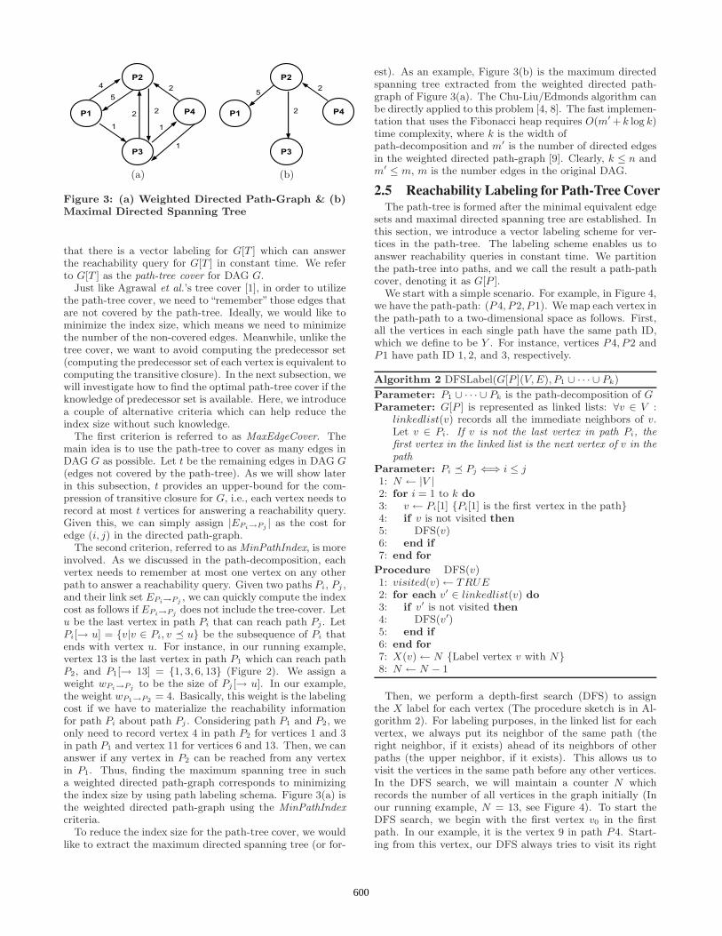
Figure 3: (a) Weighted Directed Path-Graph & (b)Maximal Directed Spanning Tree

that there is a vector labeling for G[T ] which can answerthe reachability query for G[T ] in constant time. We referto G[T ] as the path-tree cover for DAG G.

Just like Agrawal et al.’s tree cover [1], in order to utilizethe path-tree cover, we need to “remember” those edges thatare not covered by the path-tree. Ideally, we would like tominimize the index size, which means we need to minimizethe number of the non-covered edges. Meanwhile, unlike thetree cover, we want to avoid computing the predecessor set(computing the predecessor set of each vertex is equivalent tocomputing the transitive closure). In the next subsection, wewill investigate how to find the optimal path-tree cover if theknowledge of predecessor set is available. Here, we introducea couple of alternative criteria which can help reduce theindex size without such knowledge.

The first criterion is referred to as MaxEdgeCover. Themain idea is to use the path-tree to cover as many edges inDAG G as possible. Let t be the remaining edges in DAG G(edges not covered by the path-tree). As we will show laterin this subsection, t provides an upper-bound for the com-pression of transitive closure for G, i.e., each vertex needs torecord at most t vertices for answering a reachability query.Given this, we can simply assign |EPi→Pj | as the cost foredge (i, j) in the directed path-graph.

The second criterion, referred to as MinPathIndex, is moreinvolved. As we discussed in the path-decomposition, eachvertex needs to remember at most one vertex on any otherpath to answer a reachability query. Given two paths Pi, Pj ,and their link set EPi→Pj , we can quickly compute the indexcost as follows if EPi→Pj does not include the tree-cover. Letu be the last vertex in path Pi that can reach path Pj . LetPi[→ u] = {v|v ∈ Pi, v � u} be the subsequence of Pi thatends with vertex u. For instance, in our running example,vertex 13 is the last vertex in path P1 which can reach pathP2, and P1[→ 13] = {1, 3, 6, 13} (Figure 2). We assign aweight wPi→Pj to be the size of Pj [→ u]. In our example,the weight wP1→P2 = 4. Basically, this weight is the labelingcost if we have to materialize the reachability informationfor path Pi about path Pj . Considering path P1 and P2, weonly need to record vertex 4 in path P2 for vertices 1 and 3in path P1 and vertex 11 for vertices 6 and 13. Then, we cananswer if any vertex in P2 can be reached from any vertexin P1. Thus, finding the maximum spanning tree in sucha weighted directed path-graph corresponds to minimizingthe index size by using path labeling schema. Figure 3(a) isthe weighted directed path-graph using the MinPathIndexcriteria.

To reduce the index size for the path-tree cover, we wouldlike to extract the maximum directed spanning tree (or for-

est). As an example, Figure 3(b) is the maximum directedspanning tree extracted from the weighted directed path-graph of Figure 3(a). The Chu-Liu/Edmonds algorithm canbe directly applied to this problem [4, 8]. The fast implemen-tation that uses the Fibonacci heap requires O(m′ + k log k)time complexity, where k is the width ofpath-decomposition and m′ is the number of directed edgesin the weighted directed path-graph [9]. Clearly, k ≤ n andm′ ≤ m, m is the number edges in the original DAG.

2.5 Reachability Labeling for Path-Tree CoverThe path-tree is formed after the minimal equivalent edge

sets and maximal directed spanning tree are established. Inthis section, we introduce a vector labeling scheme for ver-tices in the path-tree. The labeling scheme enables us toanswer reachability queries in constant time. We partitionthe path-tree into paths, and we call the result a path-pathcover, denoting it as G[P ].

We start with a simple scenario. For example, in Figure 4,we have the path-path: (P4, P2, P1). We map each vertex inthe path-path to a two-dimensional space as follows. First,all the vertices in each single path have the same path ID,which we define to be Y . For instance, vertices P4, P2 andP1 have path ID 1, 2, and 3, respectively.

Algorithm 2 DFSLabel(G[P ](V, E), P1 ∪ · · · ∪ Pk)

Parameter: P1 ∪ · · · ∪ Pk is the path-decomposition of GParameter: G[P ] is represented as linked lists: ∀v ∈ V :

linkedlist(v) records all the immediate neighbors of v.Let v ∈ Pi. If v is not the last vertex in path Pi, thefirst vertex in the linked list is the next vertex of v in thepath

Parameter: Pi � Pj ⇐⇒ i ≤ j1: N ← |V |2: for i = 1 to k do3: v ← Pi[1] {Pi[1] is the first vertex in the path}4: if v is not visited then5: DFS(v)6: end if7: end for

Procedure DFS(v)1: visited(v)← TRUE2: for each v′ ∈ linkedlist(v) do3: if v′ is not visited then4: DFS(v′)5: end if6: end for7: X(v)← N {Label vertex v with N}8: N ← N − 1

Then, we perform a depth-first search (DFS) to assignthe X label for each vertex (The procedure sketch is in Al-gorithm 2). For labeling purposes, in the linked list for eachvertex, we always put its neighbor of the same path (theright neighbor, if it exists) ahead of its neighbors of otherpaths (the upper neighbor, if it exists). This allows us tovisit the vertices in the same path before any other vertices.In the DFS search, we will maintain a counter N whichrecords the number of all vertices in the graph initially (Inour running example, N = 13, see Figure 4). To start theDFS search, we begin with the first vertex v0 in the firstpath. In our example, it is the vertex 9 in path P4. Start-ing from this vertex, our DFS always tries to visit its right

600

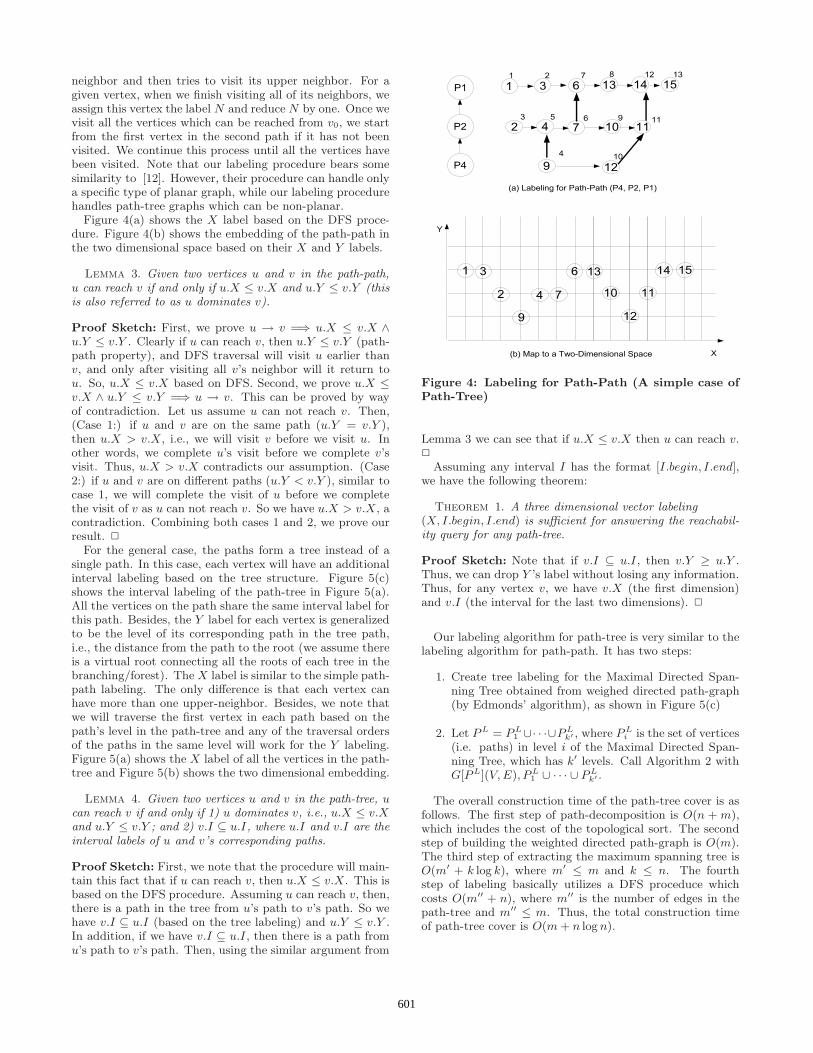
neighbor and then tries to visit its upper neighbor. For agiven vertex, when we finish visiting all of its neighbors, weassign this vertex the label N and reduce N by one. Once wevisit all the vertices which can be reached from v0, we startfrom the first vertex in the second path if it has not beenvisited. We continue this process until all the vertices havebeen visited. Note that our labeling procedure bears somesimilarity to [12]. However, their procedure can handle onlya specific type of planar graph, while our labeling procedurehandles path-tree graphs which can be non-planar.

Figure 4(a) shows the X label based on the DFS proce-dure. Figure 4(b) shows the embedding of the path-path inthe two dimensional space based on their X and Y labels.

Lemma 3. Given two vertices u and v in the path-path,u can reach v if and only if u.X ≤ v.X and u.Y ≤ v.Y (thisis also referred to as u dominates v).

Proof Sketch: First, we prove u → v =⇒ u.X ≤ v.X ∧u.Y ≤ v.Y . Clearly if u can reach v, then u.Y ≤ v.Y (path-path property), and DFS traversal will visit u earlier thanv, and only after visiting all v’s neighbor will it return tou. So, u.X ≤ v.X based on DFS. Second, we prove u.X ≤v.X ∧ u.Y ≤ v.Y =⇒ u → v. This can be proved by wayof contradiction. Let us assume u can not reach v. Then,(Case 1:) if u and v are on the same path (u.Y = v.Y ),then u.X > v.X, i.e., we will visit v before we visit u. Inother words, we complete u’s visit before we complete v’svisit. Thus, u.X > v.X contradicts our assumption. (Case2:) if u and v are on different paths (u.Y < v.Y ), similar tocase 1, we will complete the visit of u before we completethe visit of v as u can not reach v. So we have u.X > v.X, acontradiction. Combining both cases 1 and 2, we prove ourresult. �

For the general case, the paths form a tree instead of asingle path. In this case, each vertex will have an additionalinterval labeling based on the tree structure. Figure 5(c)shows the interval labeling of the path-tree in Figure 5(a).All the vertices on the path share the same interval label forthis path. Besides, the Y label for each vertex is generalizedto be the level of its corresponding path in the tree path,i.e., the distance from the path to the root (we assume thereis a virtual root connecting all the roots of each tree in thebranching/forest). The X label is similar to the simple path-path labeling. The only difference is that each vertex canhave more than one upper-neighbor. Besides, we note thatwe will traverse the first vertex in each path based on thepath’s level in the path-tree and any of the traversal ordersof the paths in the same level will work for the Y labeling.Figure 5(a) shows the X label of all the vertices in the path-tree and Figure 5(b) shows the two dimensional embedding.

Lemma 4. Given two vertices u and v in the path-tree, ucan reach v if and only if 1) u dominates v, i.e., u.X ≤ v.Xand u.Y ≤ v.Y ; and 2) v.I ⊆ u.I, where u.I and v.I are theinterval labels of u and v’s corresponding paths.

Proof Sketch: First, we note that the procedure will main-tain this fact that if u can reach v, then u.X ≤ v.X. This isbased on the DFS procedure. Assuming u can reach v, then,there is a path in the tree from u’s path to v’s path. So wehave v.I ⊆ u.I (based on the tree labeling) and u.Y ≤ v.Y .In addition, if we have v.I ⊆ u.I , then there is a path fromu’s path to v’s path. Then, using the similar argument from

Figure 4: Labeling for Path-Path (A simple case ofPath-Tree)

Lemma 3 we can see that if u.X ≤ v.X then u can reach v.�

Assuming any interval I has the format [I.begin, I.end],we have the following theorem:

Theorem 1. A three dimensional vector labeling(X, I.begin, I.end) is sufficient for answering the reachabil-ity query for any path-tree.

Proof Sketch: Note that if v.I ⊆ u.I , then v.Y ≥ u.Y .Thus, we can drop Y ’s label without losing any information.Thus, for any vertex v, we have v.X (the first dimension)and v.I (the interval for the last two dimensions). �

Our labeling algorithm for path-tree is very similar to thelabeling algorithm for path-path. It has two steps:

1. Create tree labeling for the Maximal Directed Span-ning Tree obtained from weighed directed path-graph(by Edmonds’ algorithm), as shown in Figure 5(c)

2. Let P L = P L1 ∪· · ·∪P L

k′ , where P Li is the set of vertices

(i.e. paths) in level i of the Maximal Directed Span-ning Tree, which has k′ levels. Call Algorithm 2 withG[P L](V, E), P L

1 ∪ · · · ∪ P Lk′ .

The overall construction time of the path-tree cover is asfollows. The first step of path-decomposition is O(n + m),which includes the cost of the topological sort. The secondstep of building the weighted directed path-graph is O(m).The third step of extracting the maximum spanning tree isO(m′ + k log k), where m′ ≤ m and k ≤ n. The fourthstep of labeling basically utilizes a DFS proceduce whichcosts O(m′′ + n), where m′′ is the number of edges in thepath-tree and m′′ ≤ m. Thus, the total construction timeof path-tree cover is O(m + n log n).

601

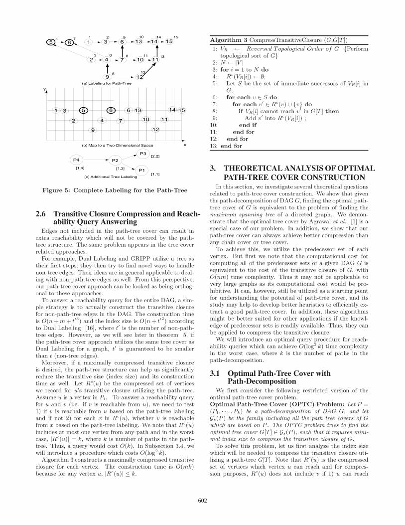
Figure 5: Complete Labeling for the Path-Tree

2.6 Transitive Closure Compression and Reach-ability Query Answering

Edges not included in the path-tree cover can result inextra reachability which will not be covered by the path-tree structure. The same problem appears in the tree coverrelated approaches.

For example, Dual Labeling and GRIPP utilize a tree astheir first steps; they then try to find novel ways to handlenon-tree edges. Their ideas are in general applicable to deal-ing with non-path-tree edges as well. From this perspective,our path-tree cover approach can be looked as being orthog-onal to these approaches.

To answer a reachability query for the entire DAG, a sim-ple strategy is to actually construct the transitive closurefor non-path-tree edges in the DAG. The construction timeis O(n + m + t′3) and the index size is O(n + t′2) accordingto Dual Labeling [16], where t′ is the number of non-path-tree edges. However, as we will see later in theorem 5, ifthe path-tree cover approach utilizes the same tree cover asDual Labeling for a graph, t′ is guaranteed to be smallerthan t (non-tree edges).

Moreover, if a maximally compressed transitive closureis desired, the path-tree structure can help us significantlyreduce the transitive size (index size) and its constructiontime as well. Let Rc(u) be the compressed set of verticeswe record for u’s transitive closure utilizing the path-tree.Assume u is a vertex in Pi. To answer a reachability queryfor u and v (i.e. if v is reachable from u), we need to test1) if v is reachable from u based on the path-tree labelingand if not 2) for each x in Rc(u), whether v is reachablefrom x based on the path-tree labeling. We note that Rc(u)includes at most one vertex from any path and in the worstcase, |Rc(u)| = k, where k is number of paths in the path-tree. Thus, a query would cost O(k). In Subsection 3.4, wewill introduce a procedure which costs O(log2 k).

Algorithm 3 constructs a maximally compressed transitiveclosure for each vertex. The construction time is O(mk)because for any vertex u, |Rc(u)| ≤ k.

Algorithm 3 CompressTransitiveClosure (G,G[T ])

1: VR ← Reversed Topological Order of G {Performtopological sort of G}

2: N ← |V |3: for i = 1 to N do4: Rc(VR[i])← ∅;5: Let S be the set of immediate successors of VR[i] in

G;6: for each v ∈ S do7: for each v′ ∈ Rc(v) ∪ {v} do8: if VR[i] cannot reach v′ in G[T ] then9: Add v′ into Rc(VR[i]) ;

10: end if11: end for12: end for13: end for

3. THEORETICAL ANALYSIS OF OPTIMALPATH-TREE COVER CONSTRUCTION

In this section, we investigate several theoretical questionsrelated to path-tree cover construction. We show that giventhe path-decomposition of DAG G, finding the optimal path-tree cover of G is equivalent to the problem of finding themaximum spanning tree of a directed graph. We demon-strate that the optimal tree cover by Agrawal et al. [1] is aspecial case of our problem. In addition, we show that ourpath-tree cover can always achieve better compression thanany chain cover or tree cover.

To achieve this, we utilize the predecessor set of eachvertex. But first we note that the computational cost forcomputing all of the predecessor sets of a given DAG G isequivalent to the cost of the transitive closure of G, withO(nm) time complexity. Thus it may not be applicable tovery large graphs as its computational cost would be pro-hibitive. It can, however, still be utilized as a starting pointfor understanding the potential of path-tree cover, and itsstudy may help to develop better heuristics to efficiently ex-tract a good path-tree cover. In addition, these algorithmsmight be better suited for other applications if the knowl-edge of predecessor sets is readily available. Thus, they canbe applied to compress the transitive closure.

We will introduce an optimal query procedure for reach-ability queries which can achieve O(log2 k) time complexityin the worst case, where k is the number of paths in thepath-decomposition.

3.1 Optimal Path-Tree Cover withPath-Decomposition

We first consider the following restricted version of theoptimal path-tree cover problem.Optimal Path-Tree Cover (OPTC) Problem: Let P =(P1, · · · , Pk) be a path-decomposition of DAG G, and letGs(P ) be the family including all the path tree covers of Gwhich are based on P . The OPTC problem tries to find theoptimal tree cover G[T ] ∈ Gs(P ), such that it requires mini-mal index size to compress the transitive closure of G.

To solve this problem, let us first analyze the index sizewhich will be needed to compress the transitive closure uti-lizing a path-tree G[T ]. Note that Rc(u) is the compressedset of vertices which vertex u can reach and for compres-sion purposes, Rc(u) does not include v if 1) u can reach

602

v through the path-tree G[T ] and 2) there is an vertexx ∈ Rc(u), such that x can reach v through the path-treeG[T ]. Given this, we can define the compressed index sizeas

Index cost =X

u∈V (G)

|Rc(u)|

(We omit the labeling cost for each vertex as it is the samefor any path-tree.) To optimize the index size, we utilize thefollowing equivalence.

Lemma 5. For any vertex v, let Tpre(v) be the immedi-ate predecessor of v on the path-tree G[T ]. Then, we have

Index cost =X

v∈V (G)

|S(v)\([

x∈Tpre(v)

(S(x) ∪ {x}))|

where S(v) includes all the vertices which can reach vertexv in DAG G.

Proof Sketch: For vertex v, if v ∈ Rc(u), thenu ∈ S(v)\(S

x∈Tpre(v)(S(x) ∪ {x})). This can be proved by

contradiction. Assume u �∈ S(v)\(Sx∈Tpre(v)(S(x) ∪ {x})).

Then there must exist a vertex w such that u can reach w inDAG G and w can reach v in the path tree. Then v shouldbe replaced by w in Rc(u), a contradiction.

For vertex u, if u ∈ S(v)\(Sx∈Tpre(v)(S(x) ∪ {x})), then

v ∈ Rc(u). This can also be proved by contradiction. As-sume v �∈ Rc(u). Then because u ∈ S(v)\(S

x∈Tpre(v)(S(x)∪{x})) we conclude u cannot reach v no matter what othervertices are in Rc(u), a contradiction. Thus, for each vertex

v ∈ Rc(u)⇐⇒ u ∈ S(v)\([

x∈Tpre(v)

(S(x) ∪ {x}))

�

Given this, we can solve the OPTC problem by utiliz-ing the predecessor sets to assign weights to the edges ofthe weighted directed path-graph in Subsection 2.4. Thus,the path-tree which corresponds to the maximum spanningtree of the weighted directed path-graph optimizes the in-dex size for the transitive closure. Consider two paths Pi, Pj

and the minimal equivalent edge set ERPi,Pj

. For each edge

(u, v) ∈ ERPi,Pj

, let v′ be the vertex which is the immediatepredecessor of v in path Pj . Then, we define the predecessorset of v with respect to u as

Su(v) = (S(u) ∪ {u})\(S(v′) ∪ {v′})If v is the first vertex in the path Pj , then we define S(v′) =∅. Given this, we define the weight from path Pi to path Pj

as

wPi→Pj =X

(u,v)∈ERPi→Pj

|Su(v)|

We refer to such criteria as OptIndex.

Theorem 2. The path-tree cover corresponding to the max-imum spanning tree from the weighted directed path-graphdefined by OptIndex achieves the minimal index size for thecompressed transitive closure among all the path-trees in Gs(P ).

Proof Sketch: We decompose Index cost utilizing the path-decomposition P = P1 ∪ · · · ∪ · · ·Pk as follows:

Index cost =X

1≤i≤k

X

v∈Pi

|S(v)\([

x∈Tpre(v)

(S(x) ∪ {x}))|

Note that S(v) ⊇ (S

x∈Tpre(v)(S(x)∪{x})). Then, minimiz-

ing the Index cost is equivalent to maximizingX

1≤i≤k

X

v∈Pi

|[

x∈Tpre(v)

(S(x) ∪ {x})|

We can further rewrite it as (vl being the vertex with largestsid in the path Pi)

X

1≤i≤k

(X

v∈Pi\{vl}|S(v) ∪ {v}|+

X

(u,v)∈ERPj→Pi

|Su(v)|)

where Pj is the parent path in the path-tree of path Pi.Since the first half of the sum is the same for the given pathdecomposition, we essentially need to maximize

X

1≤i≤k

X

(u,v)∈ERPi→Pj

|Su(v)| =X

1≤i≤k

wPi→Pj

�

Recall that in Agrawal’s optimal tree cover algorithm [1],to build the tree, for each vertex v in DAG G, essentiallythey choose its immediate predecessor u with the maximalnumber of predecessors as its parent vertex, i.e.,

|S(u)| ≥ |S(x)|, ∀x ∈ in(v), u ∈ in(v)

Given this, we can easily see that if the path decompositiontreats each vertex in G as an individual path, then we havethe optimal tree cover algorithm from Agrawal et al. [1].

Theorem 3. The optimal tree cover algorithm [1] is aspecial case of path-tree construction when each vertex corre-sponds to an individual path and the weighted directed path-graph utilizes the OptIndex criteria.

Proof Sketch: Note that for any vertices u and v such that(u, v) ∈ E(G), then the weight on the edge (u, v) in theweighted directed path-graph (each path is a single vertex)is wu,v = |S(u) ∪ {u}|. �

3.2 Optimal Path-DecompositionTheorem 2 shows the optimal path-tree cover for the given

path-decomposition. A follow-up question is then how tochoose the path-decomposition which can achieve overall op-timality. This problem, however, remains open at this point(undecided between P and NP ). Instead, we ask the fol-lowing question.Optimal Path-Decomposition (OPD) Problem: As-suming we utilize only the path-decomposition to compressthe transitive closure (in other words, no cross-path edges),the OPD problem is to find the optimal path-decompositionwhich can maximally compress the transitive closure.

There are clearly cases where the optimal path-decompositiondoes not lead to the perfect path-tree that alone can an-swer all the reachability queries. This nevertheless providesa good heuristic to choose a good path-decomposition inthe case where the predecessor sets are available. Note thatthe OPD problem is different from the chain decompositionproblem in [11], where the goal is to find the minimal widthof the chain decomposition.

We map this problem to the minimal-cost flow problem [10].We transform the given DAG G into a network GN (referredto as the flow-network for G) as follows. First, each vertexv in G is split into two vertices sv and ev, and we insert asingle edge connecting sv to ev. We assign the cost of such

603

an edge F (sv, ev) to be 0. Then, for an edge (u, v) in G,we map it to (eu, sv) in GN . The cost of such an edge isF (eu, sv) = −|S(u)∪{u}|, where S(u) is the predecessor setof u. Finally, we add a virtual source vertex and a virtualsink vertex. The virtual source vertex is connected to anyvertex sv in GN with cost 0. Similarly, each vertex ev is con-nected to the sink vertex with cost being zero. The capacityof each edge in GN is one (C(x, y) = 1). Thus, each edgecan take maximally one unit of flow, and correspondinglyeach vertex can belong to one and only one path.

Let c(x, y) be the amount (0 or 1) of flow over edge (x, y)in GN . The cost of the flow over the edge is c(x, y)·F (x, y),where c(x, y) ≤ C(x, y). We would like to find a set of flowswhich go through all the vertex-edges (sv, ev) and whoseoverall cost is minimal. We can solve it using an algorithmfor the minimum-cost flow problem for the case where theamount of flow being sent from the source to the sink isgiven. Let i-flow be the solution for the minimum-cost flowproblem when the total amount of flow from the source tothe sink is fixed at i units. We can then vary the amountof flow from 1 to n units and choose the largest one i-flowwhich achieves the minimum cost. It is apparent that i-flowgoes through all the vertex-edges (sv, ev).

Theorem 4. Let GN be the flow-network for DAG G.Let Fk be the minimal cost of the amount of k-flow from thesource to the sink, 1 ≤ k ≤ n. Let i-flow from the source tothe sink minimize all the n-flow, Fi ≤ Fk, 1 ≤ k ≤ n. Thei-flow corresponds to the best index size if we utilize only thepath-decomposition to compress the transitive closure.

Proof Sketch: First, we can prove that for any given i-flow, where i is an integer, the flow with minimal-cost willpass each edge either with 1 or 0 (similar to the Integer Flowproperty [6]). Basically, the flow can be treated as a binaryflow. In other words, any flow going from the source to thesink will not split into branches (note that each edge hasonly capacity one). Thus, applying Theorem 2, we can seethat the total cost of the flow (multiplied by negative one)corresponds to the savings for the Index cost

X

1≤i≤k

(X

v∈Pi\{vl}|S(v) ∪ {v}|) =

X

(u,v)∈GN

c(u, v)× F (u, v)

where vl is the vertex with largest sid in path Pi. Then,let i-flow be the one which achieves minimal cost (the mostnegative cost) from the source to the sink. Thus, when weinvoke the algorithm which solves the minimal-cost maximalflow, we will achieve the minimal cost with i-flow. It isapparent that the i-flow goes through all the vertex-edges(sv, ev) because i is largest. Thus, we identify the flow andfind our path-decomposition. �

Note that there are several algorithms which can solvethe minimal-cost maximal-flow problem with different timecomplexities. Interested readers can refer to [10] for moredetails. Our methods can utilize any of these algorithms.

3.3 Superiority of Path-Tree Cover ApproachIn the following, we consider how to build a path-tree

which utilizes the existing chain decomposition or tree cover(if they are already computed) to achieve better compressionresults. Note that both chain decomposition and tree coverapproaches are generally as expensive as the computation oftransitive closure.

A major difference between chain decomposition and path-decomposition is that each path Pi in the path-decompositionis a subgraph of G. However, a chain may not be a subgraphof G. It is a subgraph of the transitive closure. Therefore,several methods developed by Jagadish actually require theknowledge of transitive closure [11]. We can easily applyany chain decomposition into our path-tree framework asfollows. For any chain Ci = (v1, · · · , vk), if (vi, vi+1) is notan edge in G, then we add (vi, vi+1) into the edge set E(G).The resulting graph G′ has the same transitive closure asG. Now, the chain decomposition of G becomes a pathdecomposition of G′ and we can then apply the path-treeconstruction based on this decomposition.

The path-tree built upon a chain decomposition C willachieve better compression than C itself (since at least onecross-path edge can be utilized to compress the transitiveclosure; see the formula in Theorem 2) if there is any edgeconnecting two chains in C in DAG G. Note that if thereare no edges connecting two chains in G, then both path-treeand chain decomposition completely represent G and thusmaximally compress G.

For any tree cover, we can also transform it into a path-decomposition. We extract the first path by taking theshortest path from the tree cover root to any of its leaves.After we remove this path, the tree will then break intoseveral subtrees. We perform the same extraction for eachsubtree until each subtree is empty. Thus, we can have thepath-decomposition based on the tree cover. In addition, wenote that there is at most one edge linking two paths.

Given this, we can prove the following theorem.

Theorem 5. For any tree cover, the path-tree cover whichuses the path-decomposition from the tree cover and is builtby OptIndex has an index size lower than or equal to theindex size of the corresponding tree cover.

Proof Sketch: This follows Theorem 2. Further, there is apath-tree cover which can represent the same shape as theoriginal tree cover, i.e., if there is an edge in the originaltree cover linking path Pi to Pj , there is a path-tree thatcan preserve its path-path relationship by adding this edgeand possibly more edges from path Pi to Pj in DAG G tothe path-tree. �

3.4 Very Fast Query ProcessingHere we describe an efficient query processing procedure

algorithm with O(log2 k) query time, where k is the num-ber of paths in the path-decomposition. We first build aninterval tree based on the intervals of each vertex in R(u) asfollows (this is slightly different from [7]): Let xmid be themedian of the end points of the intervals. Let u.I.begin andu.I.end be the starting point and ending point of the inter-val u.I , respectively. We define the interval tree recursively.The root node v of the tree stores xmid, such that

Ileft = {u|u.I.end < xmid}Imid = {u|xmid ∈ u.I}Iright = {u|u.I.begin > xmid}

Then, the left subtree of v is an interval tree for the setof Ileft and the right subtree of v is an interval tree forthe set of Iright. We store Imid only once and order it byu.X (the X label of the vertices in Imid). This is the keydifference between our interval tree and the standard one

604

from [7]. In addition, when Imid = ∅, the interval tree isa leaf. Following [7], we can easily construct in O(k log k)time an interval tree using O(k) storage and depth O(log k).

Algorithm 4 Query(r,v)

1: if r is not a leaf then2: Perform BinarySearch to find a vertex w on r.Imid

whose w.X is the closest one such that w.X ≤ v.X3: else4: return FALSE;5: end if6: if v.I ⊆ w.I then7: return TRUE;8: end if9: if v.I.end < r.xmid then

10: Query(r.left,v);11: else12: if v.I.begin > r.xmid then13: Query(r.right,v);14: end if15: end if

The query procedure using this interval tree is shown inAlgorithm 4 when u does not reach v through the path-tree. The complexity of the algorithm is O(log2 k). Thecorrectness of the Algorithm 4 can be proved as follows.

Lemma 6. For the case where u cannot reach v using onlythe path-tree, then Algorithm 4 correctly answer the reacha-bility query.

Proof Sketch: The key property is that for any two ver-tices w and w′ in Imid, either w.I ⊆ w′.I or w′.I ⊆ w.I .This is because the intervals are extracted from the treestructure, and it is easy to see that:

w.I ∩ w′.I �= ∅ ⇒ (w.I ⊆ w′.I) ∨ (w′.I ⊆ w.I)

Thus, we can order the intervals based on the inclusion rela-tionship. Further, if w.I ⊆ w′.I , then we have w.X < w′.X(Otherwise, we can drop w.I if w.X > w′.X). Followingthis, we can see that for any w from Line 2 if w.I does notinclude v.I , then no other vertex in Imid can include v.Iwith w.X ≤ v.X. �

4. EXPERIMENTSIn this section, we empirically evaluate our path-tree cover

approach on both real and synthetic datasets. We are par-ticularly interested in the following two questions:

1. What is the compression rate of the path-tree coverapproach, compared to that of the optimal tree coverapproach?

2. What are the construction time and query time forthe path-tree approach, compared to those of existingapproaches?

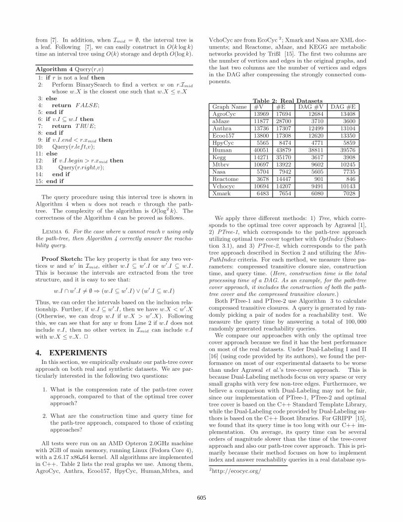
All tests were run on an AMD Opteron 2.0GHz machinewith 2GB of main memory, running Linux (Fedora Core 4),with a 2.6.17 x86 64 kernel. All algorithms are implementedin C++. Table 2 lists the real graphs we use. Among them,AgroCyc, Anthra, Ecoo157, HpyCyc, Human,Mtbra, and

VchoCyc are from EcoCyc 2; Xmark and Nasa are XML doc-uments; and Reactome, aMaze, and KEGG are metabolicnetworks provided by Trißl [15]. The first two columns arethe number of vertices and edges in the original graphs, andthe last two columns are the number of vertices and edgesin the DAG after compressing the strongly connected com-ponents.

Table 2: Real DatasetsGraph Name #V #E DAG #V DAG #EAgroCyc 13969 17694 12684 13408aMaze 11877 28700 3710 3600Anthra 13736 17307 12499 13104Ecoo157 13800 17308 12620 13350HpyCyc 5565 8474 4771 5859Human 40051 43879 38811 39576Kegg 14271 35170 3617 3908Mtbrv 10697 13922 9602 10245Nasa 5704 7942 5605 7735Reactome 3678 14447 901 846Vchocyc 10694 14207 9491 10143Xmark 6483 7654 6080 7028

We apply three different methods: 1) Tree, which corre-sponds to the optimal tree cover approach by Agrawal [1],2) PTree-1, which corresponds to the path-tree approachutilizing optimal tree cover together with OptIndex (Subsec-tion 3.1), and 3) PTree-2, which corresponds to the pathtree approach described in Section 2 and utilizing the Min-PathIndex criteria. For each method, we measure three pa-rameters: compressed transitive closure size, constructiontime, and query time. (Here, construction time is the totalprocessing time of a DAG. As an example, for the path-treecover approach, it includes the construction of both the path-tree cover and the compressed transitive closure.)

Both PTree-1 and PTree-2 use Algorithm 3 to calculatecompressed transitive closures. A query is generated by ran-domly picking a pair of nodes for a reachability test. Wemeasure the query time by answering a total of 100, 000randomly generated reachability queries.

We compare our approaches with only the optimal treecover approach because we find it has the best performanceon most of the real datasets. Under Dual-Labeling I and II[16] (using code provided by its authors), we found the per-formance on most of our experimental datasets to be worsethan under Agrawal et al.’s tree-cover approach. This isbecause Dual-Labeling methods focus on very sparse or verysmall graphs with very few non-tree edges. Furthermore, webelieve a comparison with Dual-Labeling may not be fair,since our implementation of PTree-1, PTree-2 and optimaltree cover is based on the C++ Standard Template Library,while the Dual-Labeling code provided by Dual-Labeling au-thors is based on the C++ Boost libraries. For GRIPP [15],we found that its query time is too long with our C++ im-plementation. On average, its query time can be severalorders of magnitude slower than the time of the tree-coverapproach and also our path-tree cover approach. This is pri-marily because their method focuses on how to implementindex and answer reachability queries in a real database sys-

2http://ecocyc.org/

605

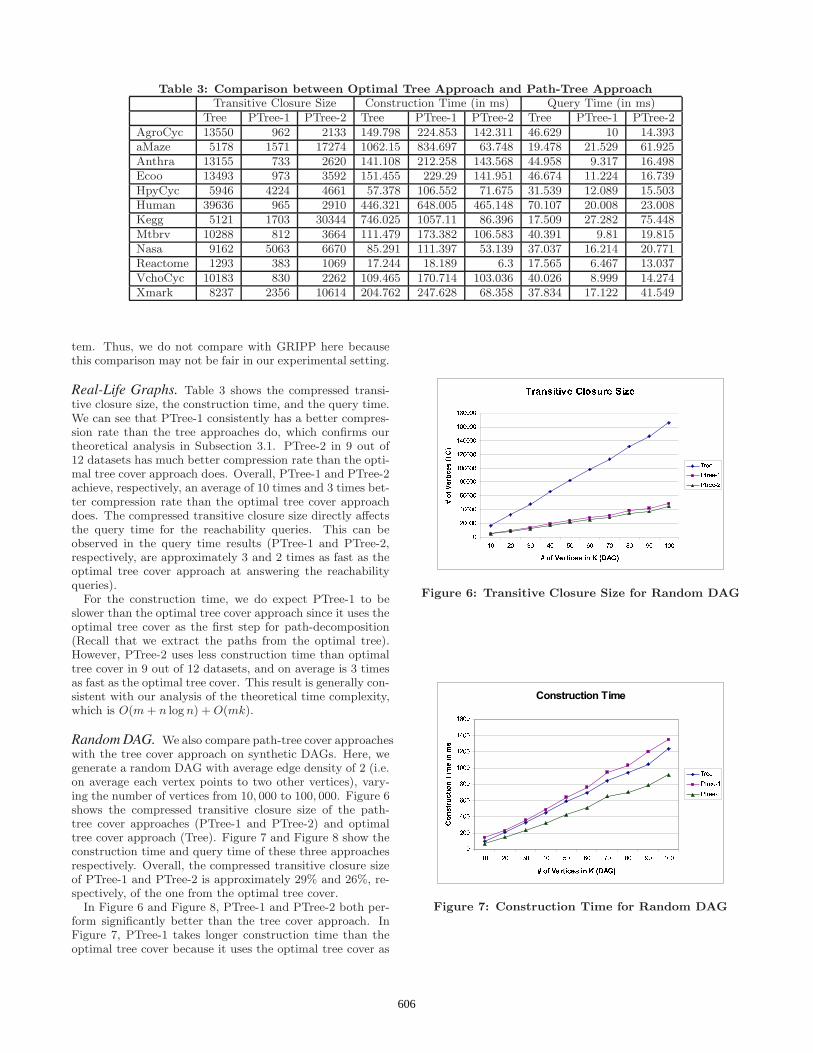
Table 3: Comparison between Optimal Tree Approach and Path-Tree ApproachTransitive Closure Size Construction Time (in ms) Query Time (in ms)

Tree PTree-1 PTree-2 Tree PTree-1 PTree-2 Tree PTree-1 PTree-2AgroCyc 13550 962 2133 149.798 224.853 142.311 46.629 10 14.393aMaze 5178 1571 17274 1062.15 834.697 63.748 19.478 21.529 61.925Anthra 13155 733 2620 141.108 212.258 143.568 44.958 9.317 16.498Ecoo 13493 973 3592 151.455 229.29 141.951 46.674 11.224 16.739HpyCyc 5946 4224 4661 57.378 106.552 71.675 31.539 12.089 15.503Human 39636 965 2910 446.321 648.005 465.148 70.107 20.008 23.008Kegg 5121 1703 30344 746.025 1057.11 86.396 17.509 27.282 75.448Mtbrv 10288 812 3664 111.479 173.382 106.583 40.391 9.81 19.815Nasa 9162 5063 6670 85.291 111.397 53.139 37.037 16.214 20.771Reactome 1293 383 1069 17.244 18.189 6.3 17.565 6.467 13.037VchoCyc 10183 830 2262 109.465 170.714 103.036 40.026 8.999 14.274Xmark 8237 2356 10614 204.762 247.628 68.358 37.834 17.122 41.549

tem. Thus, we do not compare with GRIPP here becausethis comparison may not be fair in our experimental setting.

Real-Life Graphs. Table 3 shows the compressed transi-tive closure size, the construction time, and the query time.We can see that PTree-1 consistently has a better compres-sion rate than the tree approaches do, which confirms ourtheoretical analysis in Subsection 3.1. PTree-2 in 9 out of12 datasets has much better compression rate than the opti-mal tree cover approach does. Overall, PTree-1 and PTree-2achieve, respectively, an average of 10 times and 3 times bet-ter compression rate than the optimal tree cover approachdoes. The compressed transitive closure size directly affectsthe query time for the reachability queries. This can beobserved in the query time results (PTree-1 and PTree-2,respectively, are approximately 3 and 2 times as fast as theoptimal tree cover approach at answering the reachabilityqueries).

For the construction time, we do expect PTree-1 to beslower than the optimal tree cover approach since it uses theoptimal tree cover as the first step for path-decomposition(Recall that we extract the paths from the optimal tree).However, PTree-2 uses less construction time than optimaltree cover in 9 out of 12 datasets, and on average is 3 timesas fast as the optimal tree cover. This result is generally con-sistent with our analysis of the theoretical time complexity,which is O(m + n log n) + O(mk).

Random DAG. We also compare path-tree cover approacheswith the tree cover approach on synthetic DAGs. Here, wegenerate a random DAG with average edge density of 2 (i.e.on average each vertex points to two other vertices), vary-ing the number of vertices from 10, 000 to 100, 000. Figure 6shows the compressed transitive closure size of the path-tree cover approaches (PTree-1 and PTree-2) and optimaltree cover approach (Tree). Figure 7 and Figure 8 show theconstruction time and query time of these three approachesrespectively. Overall, the compressed transitive closure sizeof PTree-1 and PTree-2 is approximately 29% and 26%, re-spectively, of the one from the optimal tree cover.

In Figure 6 and Figure 8, PTree-1 and PTree-2 both per-form significantly better than the tree cover approach. InFigure 7, PTree-1 takes longer construction time than theoptimal tree cover because it uses the optimal tree cover as

Figure 6: Transitive Closure Size for Random DAG

Figure 7: Construction Time for Random DAG

606

Figure 8: Query Time for Random DAG

the first step for path-decomposition. PTree-2 takes shorterconstruction time than the optimal tree cover as indicatedby our theoretical analysis.

In the random DAG tests, PTree-2 has slightly smallertransitive closure size and shorter query time than PTree-1 does, whereas in the real dataset tests, PTree-1 has thesmaller size and query time. We conjecture this is becausemany real datasets have tree-like structures while randomDAGs do not. Therefore, tree cover and PTree-1 fit verywell for these real datasets but less well for random DAGs.It also suggests that the MinPathIndex criteria may be wellsuited for DAGs that lack a tree-like structure.

5. CONCLUSIONIn this paper, we introduce a novel path-tree structure

to assist with the compression of transitive closure and an-swering reachability queries. Our path-tree generalizes thetraditional tree cover approach and can produce a bettercompression rate for the transitive closure. We believe ourapproach opens up new possibilities for handling reachabilityqueries on large graphs. Path-tree also has the potential tointegrate with other existing methods, such as Dual-labelingand GRIPP, to further improve the efficiency of reachabilityquery processing. In the future, we will develop disk-basedpath-tree approaches for reachability queries.

6. ACKNOWLEDGMENTSThe authors would like to thank Silke Trißl for provid-

ing the GRIPP code and datasets, Jeffrey Xu Yu for pro-viding implementations of various reachability algorithms,Victor Lee, David Fuhry and Chibuike Muoh for suggestingmanuscript revisions, and the anonymous reviewers for theirvery helpful comments.

7. REPEATABILITY ASSESSMENT RESULTA previous version of the code and results were validated

for repeatability by the repeatability committee; the resultsin these conference proceedings reflect a later (improved)version, and this version has been archived.

Code and data used in the paper are available athttp://www.sigmod.org/codearchive/sigmod2008/

8. REFERENCES[1] R. Agrawal, A. Borgida, and H. V. Jagadish. Efficient

management of transitive relationships in large dataand knowledge bases. In SIGMOD, pages 253–262,1989.

[2] Li Chen, Amarnath Gupta, and M. Erdem Kurul.Stack-based algorithms for pattern matching on dags.In VLDB ’05: Proceedings of the 31st internationalconference on Very large data bases, pages 493–504,2005.

[3] Jiefeng Cheng, Jeffrey Xu Yu, Xuemin Lin, HaixunWang, and Philip S. Yu. Fast computation ofreachability labeling for large graphs. In EDBT, pages961–979, 2006.

[4] Y. J. Chu and T. H. Liu. On the shortest arborescenceof a directed graph. Science Sinica, 14:1396–1400,1965.

[5] Edith Cohen, Eran Halperin, Haim Kaplan, and UriZwick. Reachability and distance queries via 2-hoplabels. In Proceedings of the 13th annual ACM-SIAMSymposium on Discrete algorithms, pages 937–946,2002.

[6] Thomas H. Cormen, Charles E. Leiserson, andRonald L. Rivest. Introduction to Algorithms. McGrawHill, 1990.

[7] Mark de Berg, M. van Krefeld, M. Overmars, andO. Schwarzkopf. Computational Geometry: Algorithmsand Applications. Springer-Verlag, second edition,2000.

[8] J. Edmonds. Optimum branchings. J. Research of theNational Bureau of Standards, 71B:233–240, 1967.

[9] H N Gabow, Z Galil, T Spencer, and R E Tarjan.Efficient algorithms for finding minimum spanningtrees in undirected and directed graphs.Combinatorica, 6(2):109–122, 1986.

[10] A. V. Goldberg, E. Tardos, and R. E. Tarjan. NetworkFlow Algorithms, pages 101–164. Springer Verlag,1990.

[11] H. V. Jagadish. A compression technique tomaterialize transitive closure. ACM Trans. DatabaseSyst., 15(4):558–598, 1990.

[12] T. Kameda. On the vector representation of thereachability in planar directed graphs. InformationProcessing Letters, 3(3), January 1975.

[13] R. Schenkel, A. Theobald, and G. Weikum. HOPI: Anefficient connection index for complex XML documentcollections. In EDBT, 2004.

[14] K. Simon. An improved algorithm for transitiveclosure on acyclic digraphs. Theor. Comput. Sci.,58(1-3):325–346, 1988.

[15] Silke Trißl and Ulf Leser. Fast and practical indexingand querying of very large graphs. In SIGMOD ’07:Proceedings of the 2007 ACM SIGMOD internationalconference on Management of data, pages 845–856,2007.

[16] Haixun Wang, Hao He, Jun Yang, Philip S. Yu, andJeffrey Xu Yu. Dual labeling: Answering graphreachability queries in constant time. In ICDE ’06:Proceedings of the 22nd International Conference onData Engineering (ICDE’06), page 75, 2006.

607