efficient denial constraint discovery with hydra - …¬cient denial constraint discovery with...
TRANSCRIPT
Efficient Denial Constraint Discovery with Hydra
Tobias BleifußHasso-Plattner-Institut
Prof.-Dr.-Helmert-Str. 2–314482 Potsdam, Germany
Sebastian KruseHasso-Plattner-Institut
Prof.-Dr.-Helmert-Str. 2–314482 Potsdam, Germany
Felix NaumannHasso-Plattner-Institut
Prof.-Dr.-Helmert-Str. 2–314482 Potsdam, Germany
ABSTRACT
Denial constraints (DCs) are a generalization of many otherintegrity constraints (ICs) widely used in databases, suchas key constraints, functional dependencies, or order depen-dencies. Therefore, they can serve as a unified reasoningframework for all of these ICs and express business rules thatcannot be expressed by the more restrictive IC types. Theprocess of formulating DCs by hand is difficult, because itrequires not only domain expertise but also database knowl-edge, and due to DCs’ inherent complexity, this process istedious and error-prone. Hence, an automatic DC discoveryis highly desirable: we search for all valid denial constraintsin a given database instance. However, due to the largesearch space, the problem of DC discovery is computation-ally expensive.
We propose a new algorithm Hydra, which overcomesthe quadratic runtime complexity in the number of tuples ofstate-of-the-art DC discovery methods. The new algorithm’sexperimentally determined runtime grows only linearly inthe number of tuples. This results in a speedup by ordersof magnitude, especially for datasets with a large numberof tuples. Hydra can deliver results in a matter of secondsthat to date took hours to compute.
PVLDB Reference Format:
Tobias Bleifuß, Sebastian Kruse, and Felix Naumann. EfficientDenial Constraint Discovery with Hydra. PVLDB, 11(3): xxxx-323, 2017.DOI: 10.14778/3157794.3157800
1. KILLING N BIRDS WITH ONE STONEThe research area of data profiling [1] has borne several
efficient algorithms to discover structural properties of data-sets. In particular, the discovery of functional dependencies(FDs) [13] and unique column combinations (UCCs) [8] haveattracted great attention. Lately, also order dependencies(ODs) [15] have been in focus. Each of these integrity con-straints (ICs) serves different applications, such as schemanormalization (FDs), key discovery (UCCs), and query op-timization (ODs).
Permission to make digital or hard copies of all or part of this work forpersonal or classroom use is granted without fee provided that copies arenot made or distributed for profit or commercial advantage and that copiesbear this notice and the full citation on the first page. To copy otherwise, torepublish, to post on servers or to redistribute to lists, requires prior specificpermission and/or a fee. Articles from this volume were invited to presenttheir results at The 44th International Conference on Very Large Data Bases,August 2018, Rio de Janeiro, Brazil.Proceedings of the VLDB Endowment, Vol. 11, No. 3Copyright 2017 VLDB Endowment 2150-8097/17/11.DOI: 10.14778/3157794.3157800
However, this state of the art suffers from two major prob-lems. First, each type of IC is of strongly limited expressive-ness. The types of rules one can observe in actual datasetsare much greater, though, as we demonstrate later in thissection. This imbalance is accounted for by proposing newIC types every now and then. Second, the different ICsare logically isolated. That is, to reason on the interactionamong ICs, e.g., for data cleaning, one has to explicitly pro-vide interaction rules. Not only is this unwieldy — it alsodoes not scale well with the number of considered IC types,but DCs can bridge that gap [4, 7].Then, why are there so many different ICs rather than
a single, general IC capable of avoiding such problems? Amajor reason is plain efficiency. For that matter, discover-ing FDs, UCCs, or ODs alone is already computationallyexpensive and the respective discovery algorithms employhighly specific data structures and pruning rules to operateefficiently. That being said, being able to efficiently discovermore general ICs could solve aforementioned problems andwould thus be very valuable.To this end, we propose Hydra, an efficient algorithm to
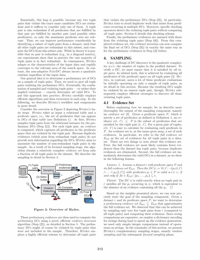
discover all valid denial constraints (DCs) in a given rela-tional dataset. But let us first define DCs and show thattheir expressiveness goes beyond UCCs, FDs, and ODs. Infew words, a DC defines a set of predicates on n tuples. Arelational instance satisfies that DC if for any n distinct tu-ples of that instance at least one predicate is violated. Inthe following, we set n = 2 and refer to the two involvedtuples as t and t′. As we show by examples below, DCs overtwo tuples are sufficient to express all of the aforementionedintegrity constraints. For reasons of rapidly increasing com-putational complexity for n > 2, as well as questionablegains, related work applies the same restriction [3].
Definition 1 (Denial constraint). Let r be a rela-tional instance with schema R(A1, . . . , An). A denial con-straint ψ is a statement of the form
∀t, t′ : ¬(
t1[A1]φ1 u
1[B1] ∧ · · · ∧ tk[Ak]φk uk[Bk]
)
with ti, ui ∈ {t, t′}, Ai, Bi ∈ {A1, . . . , An} and φi ∈ {=, 6=, <,≤, >,≥}. The different clauses in the conjunctionare referred to as predicates. The instance r satisfies ψif and only if ψ is satisfied for any two distinct tuples tand t′ ∈ r. A DC is trivial if it is valid for any possibleinstance. Furthermore, a DC ψ is (set-)minimal, if no DCwhose predicates are a subset of ψ’s predicates is valid on r.
Let us demonstrate the expressiveness of DCs with the ex-ample dataset from Table 1 in combination with some valid
311
311-
ψ1 : ∀t, t′ : ¬
(
t[Name] = t′[Name] ∧ t[Hired] = t′[Hired])
ψ2 : ∀t, t′ : ¬
(
t[Department] = t′[Department] ∧ t[D-Code] 6= t′[D-Code])
ψ3 : ∀t, t′ : ¬
(
t[ID] ≤ t′[ID] ∧ t[Hired] > t′[Hired])
ψ4 : ∀t, t′ : ¬
(
t[D-Code] = t′[D-Code] ∧ t[Hired] < t′[Hired] ∧ t[Salary] > t′[Salary])
Figure 1: A number of example DCs that hold in our example dataset (Table 1).
Table 1: Example dataset with staff data.
ID Name Department D-Code Hired Salary
t1 103 J. Miller Sales SAL 2008 3,200t2 197 J. Miller Accounting ACT 2012 3,500t3 338 P. Smith Sales SAL 2012 2,900t4 631 S. Blake Accounting ACT 2016 3,200t5 664 P. Dean Sales SAL 2016 2,700
DCs shown in Figure 1. Amongst others, Name and Hiredform a key candidate, i.e., a UCC. This fact is captured bythe DC ψ1. Further, we observe that Department determinesD-Code, that is, the FD Department → D-Code holds. ThisFD is equivalent to the DC ψ2. As a third IC, we note thatthe staff IDs reflect when an employee has been hired. Thus,we have the OD ID→≤ Hired, which can be expressed as ψ3.In addition, a closer look reveals a further, more intricateconstraint: For any two employees from the same depart-ment, the newer employee should not earn more than theolder. While neither UCCs, nor FDs, nor ODs can expressthis constraint, the DC ψ4 naturally captures it. This showsthe superiority of DCs over the specific IC types.
Problem statement. Nevertheless, automatically discov-ering all DCs in a dataset is a highly challenging task: givena relational instance r and a predicate space P , we wantto find all non-trivial, set-minimal DCs valid on r that canbe expressed using only predicates in P . At first, the num-ber of candidate DCs grows extremely fast with the numberof attributes — in fact, super-exponential! Furthermore,comparing all tuple pairs to verify DCs can be prohibitive:Although, this is only of quadratic complexity w.r.t. thenumber of tuples, there are usually orders of magnitudesmore tuples than attributes in a dataset. Our algorithmHydra mitigates these scalability traps. In fact, we makethe following major contributions:
1. We propose to first approximate the DCs for a datasetand then correct any incorrect results (Section 3). Thisavoids the comparison of all tuple pairs. In particular,we prove this idea to be sound and complete (Sec-tion 6.1).
2. We devise a technique to quickly approximate the DCsin a dataset while looking only at a small fraction of alltuple pairs. This comprises the careful choice of tuplesto compare (Section 4) and the efficient conversion ofcomparison results to approximated DCs (Section 5).
3. We explain a proceeding to efficiently determine allviolations of a dataset w.r.t. the approximated DCs.Combined with the above mentioned conversion algo-rithm, we quickly turn the set of approximate DCs tothe set of actual DCs (Section 6).
4. Finally, we exhaustively evaluate the efficiency of Hy-dra (Section 7).
In addition, we discuss related work in Section 2 and sum-marize as well as conclude in Section 8.
2. RELATED WORKAlthough the research area of data profiling has produced
various dependency discovery algorithms [1], the discoveryof denial constraints (DCs) has not received much attentionso far. Therefore, this section looks at related dependencydiscovery algorithms in a broader sense.
DC discovery. The first and only other DC discovery al-gorithm is FastDC [3], which is also our evaluation baseline.It discovers DCs in two major phases: At first, all tuples ina given dataset are compared pairwise to form the evidenceset. Then, by searching a minimal cover for this evidenceset, FastDC constructs DCs that are not violated by anyfound evidence. This strategy is much slower than that ofHydra for two reasons. First, the comparison of all tuplepairs is very expensive. Second, Hydra proposes a novel,more efficient algorithm to derive DCs from the evidenceset. Besides their basic approach, the authors of FastDCprovide two modifications of their algorithm. A-FastDC isable to detect approximate DCs, which may be partially vio-lated, and C-FastDC allows for constants in the predicatesof the DCs. We note that the modifications for C-FastDCare compatible with Hydra. Furthermore, Hydra couldbe in principle adapted to discover approximate DCs. Weoutline the necessary changes in Section 8.
UCC/FD/OD discovery. As explained in Section 1,DCs subsume various other integrity constraints, in partic-ular UCCs, FDs, and ODs. Hence, Hydra is a valid substi-tute for any of their discovery algorithms. Nonetheless, wecan identify commonalities of Hydra and those specificallytailored algorithms. Generally speaking, Hydra belongs tothe class of algorithms that are based on pairwise tuple com-parisons, which comprises, e.g., Gordian for UCC discov-ery [14], and Fdep for FD discovery [6], but no known ODdiscovery algorithm. In particular, the idea to approximateICs by repeatedly sampling tuple pairs has been successfullyapplied for FDs [2, 13]. However, sampling for DCs is morecomplex, because DCs involve inequality predicates. Also,there is no equivalent for the completion strategy for FDsvia stripped partitions [9]. Hence, a completely new com-pletion strategy is required. Another recent incentive for ef-ficiency improvements are holistic profiling algorithms thatdiscover multiple IC types in a single run, thereby savingoverhead [5]. This property applies to Hydra, too.
3. OVERVIEW OF HYDRAMany IC discovery algorithms compare all tuple pairs in a
dataset to collect every possible violation of their respectiveIC type. From those violations, the actual ICs can then beinferred [3, 6, 14]. However, those algorithms scale poorlywith the number of tuples — all tuple pairs incur quadraticcomplexity. Hydra is specifically designed to not compareall tuple pairs and, hence, to avoid this quadratic trap whendiscovering all DCs.
312
Essentially, this leap is possible, because any two tuplepairs that violate the exact same candidate DCs are redun-dant and it suffices to consider only one of them. A tuplepair is also redundant if all predicates that are fulfilled bythat pair are fulfilled by another pair (and possibly otherpredicates), so only the maximum predicate sets are rele-vant. Thus, we can improve performance considerably byidentifying a subset of tuple pairs from a dataset, such thatall other tuple pairs are redundant to this subset, and com-pute the DCs from this subset only. While in theory it is pos-sible that no pair is redundant (e.g., in a diagonal matrix),our experiments show that in practice the vast majority oftuple pairs is in fact redundant. In consequence, Hydraadapts to the characteristics of the input data and rapidlyconverges to the relevant area of the search space. In con-trast, the non-adaptive FastDC always incurs a quadraticruntime regardless of the input data.
Our general idea is to determine a preliminary set of DCson a sample of tuple pairs. Then, we need to spot all tuplepairs violating the preliminary DCs. Eventually, the combi-nation of sampled and violating tuple pairs — or rather theirimplied violations — exactly determine all valid DCs. Toput this approach into practice, Hydra carefully employsefficient algorithms and data structures in each step. In thefollowing, we describe Hydra’s workflow and componentsin more detail.
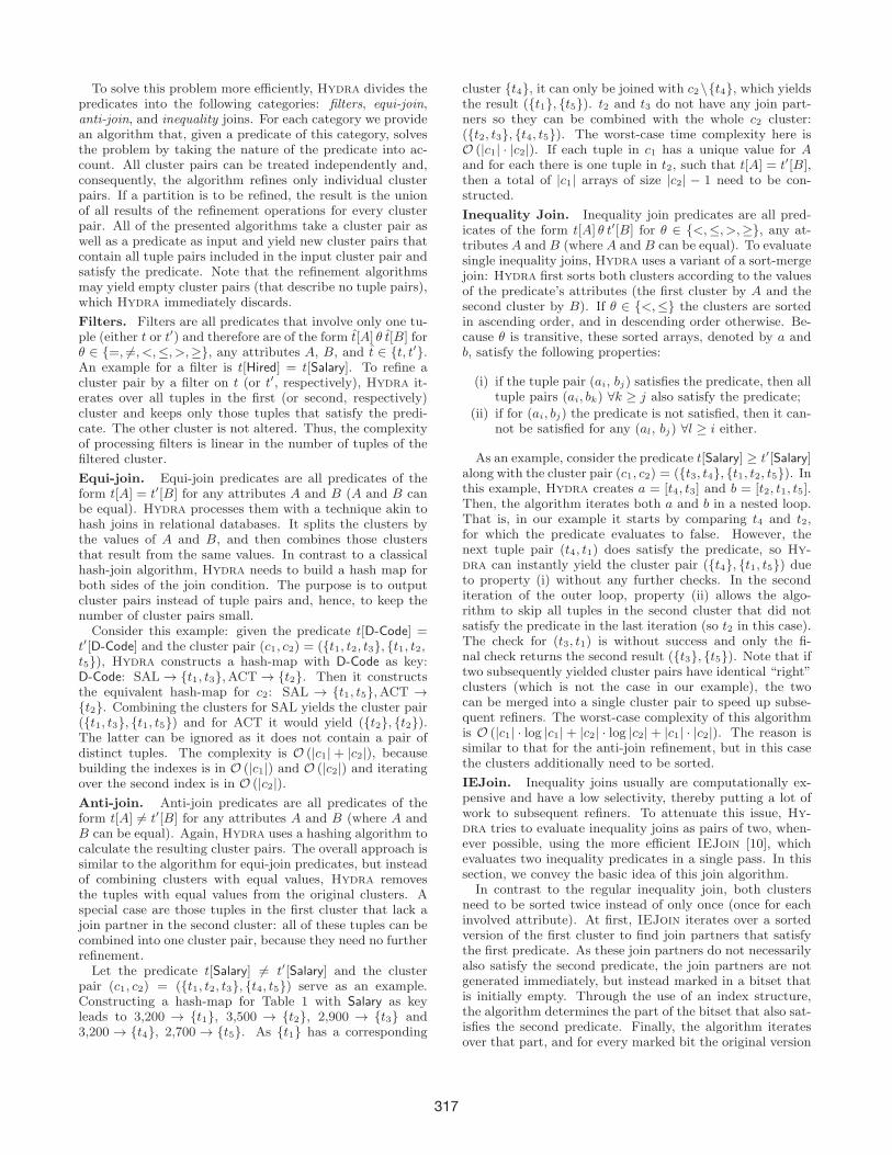
Consider the overview in Figure 2 depicting Hydra’s ba-sic steps. Hydra takes as input a relational table and apredicate space, i.e., the set of predicates that can appearin DCs of that table (see Definition 1). At first, Hydrasamples tuple pairs from the relational instance for the pre-liminary DCs (Step (1)). For each tuple pair, an evidenceis computed, which captures all predicates in the predicatespace that are violated by the tuple pair. Because duplicateevidences (which arise from redundant tuple pairs) do notprovide new information regarding the DCs, Hydra aims tomaximize the number of non-redundant tuple pairs in thesample. As a result of its focused sampling stage, the algo-rithm obtains a relatively complete evidence set from onlya fraction of all tuple pairs in the dataset. We describe thesampling in detail in Section 4.
Sampling Evidence Inversion
Dataset
Violation Detection
(1) Tuple pairs
(2) Preliminary evidences
(3) Preliminary DCs(3) Selec-
tivities
(3) Tuples
∀t,t’: …∀t,t’: …∀t,t’: …
∀t,t’: …
∀t,t’: …
∀t,t’: …
∀t,t’: …
(4) Complete
evidences (5) Final
DCs
Figure 2: Overview of Hydra.
These preliminary evidences are then used to compute thepreliminary DCs using a novel, efficient evidence inversionalgorithm (Step (2)), as detailed in Section 5. The prelim-inary DCs might of course be violated by tuple pairs thatwere not included in the sample. Therefore, Hydra em-ploys a highly efficient scheme to determine all tuple pairs
that violate the preliminary DCs (Step (3)). In particular,Hydra tries to avoid duplicate work that arises from predi-cates recurring in multiple DCs. Moreover, specific checkingoperators detect the violating tuple pairs without comparingall tuple pairs. Section 6 details this checking scheme.Finally, the preliminary evidences are unioned with those
from the violating tuple pairs (Step (4)). From this com-pleted evidence set, the evidence inversion can now computethe final set of DCs (Step (5)) in exactly the same way asfor the preliminary evidences in Step (2) before.
4. SAMPLINGA key challenge of DC discovery is the quadratic complex-
ity w.r.t. the number of tuples in the profiled dataset: Toverify a DC, we must ensure that it is satisfied by all tu-ple pairs. In related work, this is achieved by evaluating allpredicates of the predicate space on all tuple pairs [3]. Hy-dra, in contrast, saves a lot of these predicate evaluationsby initially operating on only a sample of tuple pairs, aswe detail in this section. Because the resulting DCs mightbe violated by an unseen tuple pair, though, Hydra sub-sequently employs efficient strategies to discover all thoseviolating tuple pairs.
4.1 Evidence SetBefore explaining how we sample, let us describe more
thoroughly the output of the sampling component, namelyan evidence set [3]. Given a predicate space P , which ismerely a set of predicates as defined in Definition 1, an ev-idence e(t, t′) ⊆ P is the subset of predicates that aresatisfied by the tuple pair (t, t′). For a given pair of tuples,e(t, t′) is easy to calculate by evaluating each predicate inP . An evidence set is, as the name gives away, a set of suchevidences. In particular, we refer to the full evidence setEfull as the set of evidences for all tuple pairs in a data-set. There are two things to note about this evidence set.First, the full evidence set most likely contains fewer evi-dences than the dataset has tuple pairs, because duplicateevidences are eliminated. Second, the full evidence set im-mediately determines the valid DCs in a dataset, as we showin the following lemma.
Lemma 1. Assume a dataset r with predicate space P andits full evidence set Efull. Then the DC ψ := ∀t, t′ : ¬
(
p1(t, t′)
∧ · · · ∧ pn(t, t′))
with predicates pi ∈ P is valid w.r.t. r, ifand only if 6 ∃e ∈ Efull : {p1, . . . , pn} ⊆ e.
Proof. The DC ψ is valid exactly when no tuple pair inr satisfies all the pi occurring in ψ, which is equivalent tothe absence of an evidence containing all the pi.
Based on the insights presented above, we can now pre-cisely state the goal of the sampling component: Given adataset r and its predicate space P , we want to determinea preliminary evidence set Epre ⊆ Efull that approximatesthe full evidence set. We observed that this can be achievedby sampling only very few tuple pairs from r (compared toall tuple pairs) and computing their evidences. Since stringcomparisons are expensive, we employ a dictionary encodingfor strings during load to speed up the evidence generation:we need only simple integer comparisons instead of opera-tions on strings. In the remainder of this section, we presentHydra’s complementary sampling stages, namely randomsampling and the subsequent focused sampling phase.
313

4.2 Random SamplingHydra starts by populating the preliminary evidence set
with evidences from randomly sampled tuple pairs. How-ever, the main purpose of this sampling stage is to estimatethe selectivity of predicates, i.e., the number of tuple pairsthat satisfy the predicate. That is, given a random pair oftuples, how likely is it to satisfy a certain predicate fromthe predicate space? Hydra’s violation detection can em-ploy the selectivities to optimize its efficiency (see Section 6).While a focused sample is biased and, thus, not well-suitedto determine selectivities, we can directly extrapolate theselectivities from a random sample.
To obtain the random sample, Hydra chooses for everytuple in the dataset k other random tuples and calculatesthe k associated evidences. Our experiments show that avalue of k = 20 is sufficient for a good selectivity estima-tion (Section 7.5.1). Consequently, the sampling effort islinear in the number of tuples — we retrieve k · |r| instead of|r| · (|r| − 1) pairs. Recall that usually an evidence set doesnot contain duplicate evidences. In case that two or morerandomly sampled tuples yield the same evidence, Hydraalso maintains a counter for that evidence to properly em-ploy them for selectivity estimation.
4.3 Focused SamplingThe random sample might not yet be sufficient to obtain
a good approximation of the full evidence set. Hence, wecomplement it with a focused sampling that tries to sam-ple tuple pairs that yield unseen evidences. Similar focusedsampling strategies have been devised in the context of FDdiscovery [2, 13]. However, those are not sufficient here, be-cause — speaking in DC vocabulary — their evidences con-sider only predicates of the form t[A] = t′[A] for some at-tribute A. In contrast, DC discovery has to consider othertypes of predicates, such as inequalities and comparisonsacross attributes.
Therefore, we devise a new focused sampling algorithminspired by FD discovery. Its core idea is to maintain a setof sampling foci, each of which is associated with a predi-cate from the predicate space. Each sampling focus furtherspecifies a sampling strategy that samples only tuple pairssatisfying that predicate. Now, we repeatedly sample ac-cording to whatever sampling focus we currently believe tohave the highest chance of yielding an unseen evidence. Atsome point, that belief falls below a certain threshold forall sampling foci. At that point, we terminate the samplingphase. In few words, the key points of this algorithm are to(i) ensure that all predicates are considered by the sampleand (ii) making the sampling sensitive to the yield of thedifferent sampling foci. We now explain how to technicallyrealize this sampling.
Sampling strategies. Hydra defines four sampling strate-gies: Within enforces predicates of the form t[A] = t′[A];Other enforces predicates of the form t[A] 6= t′[A]; andBack and Forth enforce predicates of the form t[A] > t′[A]and t[A] < t′[A], respectively. Note that Within, Back,and Forth are implicit strategies for the predicates with ≤and ≥.To efficiently sample according to these four strategies,
Hydra initially clusters tuples individually according to eachattribute. That is, for each attribute we obtain a set of clus-ters, each of which is a set of references to tuples that sharethe same value in the respective attribute. If the operators
< and > are defined on the considered attribute, the clustersare further ordered according to the values they represent.For instance, the attribute Salary from Table 1 defines theordered clustering ({t5}, {t3}, {t1, t4}, {t2}).Given an attribute A with its clustering, we can now eas-
ily apply any sampling strategy: For each tuple index ti, wepick a random partner tuple index tj (if any) from the same(Within) or different clusters (Other, Back, Forth), re-trieve the actual tuples for each (ti, tj), and calculate the ev-idences. For instance, if we want to apply the Back strategyto the attribute Salary and currently have ti = t4, then theclustering tells us that we have to sample tj from the pre-ceding clusters {t5} or {t3}. Assume, we sample t3, we thenneed to calculate the evidence e(t4, t3). The reader mighthave noticed that we do not define sampling strategies forpredicates that compare two distinct attributes A and B.While technically this would need only a mapping of theclusters of A to their position in the ordered cluster of B,we omit it, simply because the sampling works sufficientlywell with the four presented strategies.� � � � � � � � � �� � � � � � � � �� ���� ������
� � � � � � � � � � � � � � � � � � � � �� � � � � � �� ! " #$ % & ' () * ( % & #$ % & ' (+ , % & , -. � / � � � � � � � � � � 0� � � � � � � � � / � � � � � � � � �1 2 3 � � � 3 � � � 45 � � � �6 7 8 9: ; � � � �$ % & ' (� � � � � �) * ( % &� � � � � �+ , % & , - � � � � � � � � � � �5 � 3 � � �� � � � � � � � � � � <� =� >� ?� @A B C D D 0A B E D D 0F B A D D 0F B G D D 0H IJ I��
Figure 3: Overview of the focused sampling.
Sampling efficiency. Having explained sampling strate-gies, we can precisely describe a sampling focus as a pair ofan attribute and a sampling strategy. As described above,Hydra’s focused sampling phase repeatedly applies the mostpromising sampling focus. We define this sampling efficiencyof a sampling focus as the number of previously unseen evi-dences it has contributed (the growth in size of the distinctevidence set), divided by the total number of evidence cal-culations (as a measure of effort) during its last application.To obtain an initial efficiency, we apply all sampling focionce in the beginning, and then insert them into a prior-ity queue that orders the sampling foci descending by theirsampling efficiency.Now, we just poll a sampling focus from that priority
queue (for example Salary Within in Figure 3), apply it(calculate for example e(t4, t1)), and obtain as a byprod-uct a new efficiency value. If that value is below a certainthreshold (0.005), we discard the sampling focus — other-wise we put it back into the priority queue. Note that thisthreshold can influence only Hydra’s runtime, but never itsresult quality. Additionally, the algorithm is quite robust forthe choice of this parameter, as shown in Section 7.5.1.
5. EVIDENCE INVERSIONAn evidence set determines a set of valid DCs, as shown
in Lemma 1. However, actually computing those DCs is achallenging problem, because even the output size can be
314

exponential in the number of attributes n. This is the case,because the set of DCs generalizes the set of minimal keys,and this set can be of size
(
nn/2
)
[8]. What is more, Hy-
dra needs to perform such evidence inversion at two points(cf. Figure 2): First, it needs to invert the preliminary evi-dence set and, eventually, the full evidence set. It is there-fore crucial to perform the inversion with a high efficiency.
Intuitively, Hydra achieves that goal as follows: Initially,we assume the most basic DCs, which contain only a singlepredicate, to be true. Then, we iterate over the evidenceset. For each evidence, we update all the DCs by addingpredicates, such that the evidence no longer violates theDC. Once all evidences have been processed, the set of DCsis valid and complete.
Algorithm 1 shows this proceeding in more detail. At first,it initializes the basic candidate DCs (Line 1) and representsthem as the sets of their predicates. For instance for Table 1,we have the candidate DC ∀t, t′ : ¬(t[Name] = t′[Name]) andrepresent it as {p} (where p(t, t′) :≡ t[Name] = t′[Name]).The function handleEvidence now iteratively updates the
tentative candidate DCs, so that they conform to the evi-dence set (Line 3). The function begins by detecting allcandidate DCs ψ− ∈ Ψ− that are violated by the cur-rent evidence e (Line 6). This is the case when e satis-fies all predicates of ψ−. Our above example candidateDC would be violated by, e.g., the evidence e(t1, t2), be-cause t1 and t2 agree in the attribute Name. However, vio-lated candidate DCs in Ψ− can be reconciled with e by sim-ply adding a predicate that is not satisfied by e (Lines 9–11). For instance, our example candidate DC can be ex-tended to ∀t, t′ : ¬(t[Name] = t′[Name] ∧ t[Department] =t′[Department]). Note that there are multiple ways to rec-oncile the candidate DCs so that Ψ might eventually grow.However, the reconciliation might yield redundant DC can-didates, which is the case when there is a valid, more generalDC. For that matter, our reconciled candidate DC might besubsumed by ∀t, t′ : ¬(t[Department] = t′[Department]) (as-suming that we have not yet processed an evidence violatingit). Thus, our algorithm actively checks and removes suchredundant DC candidates (Line 10). Let us show that thisalgorithm is sound and complete.
Theorem 1. Given a predicate space P and evidence setE, Algorithm 1 determines a sound, complete, and minimalset of DCs w.r.t. E.
Proof. (Sound) Suppose a DC ψ in the output is notcorrect, i.e., an evidence e ∈ E fulfills all of its predicates(ψ ⊆ e). handleEvidence exchanges only DCs in Ψ with su-perset DCs, i.e., valid DCs can only grow due to an evidence,never shrink. Thus, for ψ to be part of the result, a subsetof ψ must be present in Ψ at all times. However, each callfor handleEvidence ensures that no DC invalidated by thecurrent evidence e remains in Ψ by removing all subsets ofe from Ψ and only adding proper supersets of e. As ψ ⊆ e,the call for handleEvidence for e = e removes all subsets ofψ and therefore ψ cannot be part of the output.(Complete) Throughout each iteration of the loop in Line 2
the following property holds: If a DC ψ is a valid, non-trivialDC, Ψ always contains a DC whose predicates are a subsetof ψ. This property obviously holds at the initialization ofΨ in Line 1. If, at some point, the last subset of ψ is re-moved in Line 7, then a new subset of ψ would be added inLine 11, as at least one superset must not be contradictory
Algorithm 1: Evidence inversion
Data: evidence set E, predicate space PResult: the set of minimal, non-trivial DCs Ψ
1 Ψ← {{p} | p ∈ P}2 for e ∈ E do3 handleEvidence (e,Ψ, P )
4 return Ψ
5 Function handleEvidence(e,Ψ, P)6 Ψ− ← {ψ− ∈ Ψ | ψ− ⊆ e}
7 Ψ← Ψ \Ψ−
8 for ψ− ∈ Ψ− do9 for p ∈ (P \ e) do
10 if 6 ∃ψ ∈ Ψ: ψ ⊆ (ψ− ∪ {p}) then11 Ψ← Ψ ∪ {ψ− ∪ {p}}
to e, otherwise ψ would not be valid. This property imme-diately leads to completeness in the sense that all valid DCscan be derived from the output.(Minimal) Suppose the DC ψ1 is valid and minimal, but
the result contains ψ2, i.e., the predicate set of ψ1 is a subsetof ψ2’s predicate set and therefore ψ2 is not minimal. Thecheck in Line 10 ensures that Ψ contains no subsets of newDCs before adding them to the result. The completenessloop invariant guarantees that Ψ always contains a subsetof ψ1, so whenever ψ2 should be added to the result, thissubset check prevents it.
6. EVIDENCE SET COMPLETIONThe output of the previous step – the preliminary DCs –
can contain DCs that are not valid on the entire relationalinstance, because the evidence that violates them was notincluded in the preliminary evidence set. Additionally, asthe inversion step outputs a minimal set of DCs, some DCsthat are actually correct can be missing in the output. Thiscan happen, because a more general, but in fact invalid DCis present in the output and thus the missing DCs are notconsidered minimal. In this section, we describe how to ar-rive at all minimal DCs given the preliminary evidence setand DCs. At first, we characterize which evidences the pre-liminary evidence set lacks to entail the complete and correctset of DCs (Section 6.1). Then, we show how to efficientlycollect exactly those missing evidences (Sections 6.2–6.4).Applying once more the evidence inversion from Section 5 tothe preliminary and newly collected evidences finally givesus the correct and complete set of DCs for the entire dataset.
6.1 The Delta Evidence SetA delta evidence set E∆ is a set of evidences that entails
the correct and complete DCs of a dataset when combinedwith the preliminary evidence set. That is, the delta evi-dence set is precisely the set of evidences that are missingfrom the preliminary set to make the result correct. Recallthat the preliminary evidence set itself entails a set of pre-liminary DCs. Interestingly, the evidences for all tuple pairsthat violate any of the preliminary DCs form such a deltaevidence set.
Theorem 2. Assume a preliminary evidence set Epre andits associated DCs Ψpre. Further assume an evidence set E∆
315

that contains the evidences for all tuple pairs that violateΨpre. Then an evidence inversion of Epre ∪ E∆ leads to thecomplete and minimal set of denial constraints.
Proof. The evidence inversion’s result is unambiguouslydetermined by the maximal evidences emax, which are not asubset of a further evidence in the same evidence set. Thisis because any DC that is precluded by some e′ ⊆ emax
is also precluded by emax. Now, let Efull denote the fullevidence set and assume that some maximal evidence emax ={p1, . . . , pn} is contained in Efull but not in Epre. In otherwords, Efull precludes the DC ψ = ∀t, t′ : ¬(p1 ∧ · · · ∧ pn),while Epre does not. Hence, there must be some DC ψpre ∈Ψpre that comprises only predicates from emax. Because thetuple pair yielding emax violates ψpre, emax is in E∆. So,we can conclude that all maximal evidences from Efull areeither included in Epre or E∆. Therefore, Efull and Epre∪E∆
entail the same DC set.
Example 1. Let us assume that our sampling did notcompare t1 and t2. Therefore, we did not find any evidencesthat contradict the DC ∀t, t′ : ¬t[Name] = t′[Name] and theDC is thus contained in our preliminary DC set Ψpre. Whenwe check this DC, we discover that the tuple pairs (t1, t2)and (t2, t1) violate that DC and we can add two new ele-ments e(t1, t2) and e(t2, t1) to our evidence set. As shownin the proof above, the evidence set is complete if we repeatthis process for every DC in Ψpre.
To employ Theorem 2 for DC discovery, we need to discoverE∆ and, hence, all tuple pairs that violate any of the pre-liminary DCs in Ψpre. A naıve approach to discover all vio-lating tuple pairs for some DC ψpre ∈ Ψpre (i) inspects eachtuple pair; (ii) determines, whether the tuple pair violatesψpre; and, if so, (iii) saves this tuple pair for the calculationof E∆. However, this approach has a runtime complexityof O(|Ψpre| · |r|
2), where |r| is the number of tuples in thedataset, and is clearly too inefficient.
Hydra tackles this challenging task to efficiently discoverE∆ on two levels. At first, it provides an efficient schemeto discover the violating tuple pairs for a single DC, by em-ploying specific data structures (Section 6.2) and dedicatedevaluation algorithms for the various predicate types (Sec-tion 6.3). Second, Hydra optimizes the checking of multipleDCs at once. This is possible, because DCs often share somepredicates, which might then need to be checked only once(Section 6.4).
6.2 Checking a single DCAssume a DC ψ = ∀t, t′ : ¬(p1 ∧ · · · ∧ pn) whose violating
tuple pairs we would like to determine. Intuitively, we canattain this as follows: We initially assume that all tuple pairsTP :=
{
(t, t′) ∈ r2 | t 6= t′}
violate ψ. Then, we iterate thepredicates in ψ in some order and for each predicate pi, weretain only those tuple pairs that satisfy pi using a refinerfunction refpi(TP) :=
{
(t, t′) ∈ TP | (t, t′) satisfies pi}
. Fi-nally, we obtain all tuple pairs (refp1 ◦ · · · ◦ refpn)(TP) thatsatisfy all predicates in ψ — these are exactly the violatingtuple pairs. We now explain how to efficiently implementthis proceeding.
Data Structures. Obviously, representing sets of tuplepairs by explicitly materializing them all is neither memoryefficient nor allows for efficient processing. Instead, Hydrauses three data structures to represent sets of tuple pairs: A
cluster is an unordered set of tuple indices. A cluster pairis an ordered pair (c1, c2) of two clusters c1 and c2. It repre-sents all tuple pairs (t, t′), such that t ∈ c1 and t′ ∈ c2 andt 6= t′. As an example, the cluster pair ({t1, t2}, {t2, t3})represents the tuple pairs (t1, t2), (t1, t3), (t2, t3). A parti-tion is a set of cluster pairs, which represents all tuple pairscontained in any of those cluster pairs.The partition representation has the advantage that many
partitions can be represented using much less memory thanwould be required by the enumeration of every tuple pair.For instance, all possible (ordered) tuple pairs in a datasetwith |r| tuples, can be represented as one partition with onlyone cluster pair, where each cluster contains all tuples. Wecall this partition that represents the cross-product of alltuples the full partition of r. This representation requiresonly 2n integers – so only linear space, as opposed to ton2−n tuple pairs for a materialization of the cross product.
Operations. Besides being a compact representation, par-titions can be employed to efficiently implement the refine-ment operation defined above. We extend the definitionabove to a new operator called partition refiner, that takesas input a set of cluster pairs and yields a set of cluster pairsthat represents all tuples pairs of the input cluster pair thatalso satisfy a predicate pi. Again, the repeated applicationfor all predicates of a DC, starting with the full partition,yields the set of all tuple pairs violating this DC. Thus, itis of major importance for Hydra to efficiently execute therefinement. The actually employed refinement strategies aredetermined by the type of the processed predicate and aredescribed in detail in Section 6.3.
Pipelining. Although partitions are a compact represen-tation of tuple pairs, they still can consume a considerableamount of memory — in particular, when there are verymany very small cluster pairs. Hydra attenuates this factby pipelining: Instead of applying the partition refiner foreach predicate one after another, Hydra rather operates onthe granularity of cluster pairs. That is, as soon as a parti-tion refiner yields a refined cluster pair, this cluster pair isdirectly fed into the partition refiner of the next predicate.As an example, consider the full partition for Table 1, whichwe want to refine with the predicate t[Name] = t′[Name].The refined partition would contain four cluster pairs, onefor each name. However, as soon as the partition refiner hasdetermined one of the cluster pairs, e.g.,
(
{t1, t2}, {t1, t2})
for J. Miller, this cluster pair can immediately be refinedfurther with other predicates (if any exist). Note that thisoptimization technique is independent of the actual refine-ment strategy.
6.3 Refinement strategiesHaving explained the utility of partition refinement to dis-
cover the violating tuple pairs for a given DC, let us now dis-cuss the actual refinement strategies. In brief, a refinementstrategy takes as input a predicate and a partition and out-puts a refined partition that contains only tuple pairs thatsatisfy the given predicate. A naıve solution to this problemcould be an algorithm that iterates over all tuple pairs in thepartition and adds each of them to the resulting partitionif the tuple pair satisfies the predicate. While this solutionwould work correctly, it certainly is not efficient. As a mat-ter of fact, this strategy would compare all tuple pairs – thisis exactly what Hydra attempts to avoid!
316
To solve this problem more efficiently, Hydra divides thepredicates into the following categories: filters, equi-join,anti-join, and inequality joins. For each category we providean algorithm that, given a predicate of this category, solvesthe problem by taking the nature of the predicate into ac-count. All cluster pairs can be treated independently and,consequently, the algorithm refines only individual clusterpairs. If a partition is to be refined, the result is the unionof all results of the refinement operations for every clusterpair. All of the presented algorithms take a cluster pair aswell as a predicate as input and yield new cluster pairs thatcontain all tuple pairs included in the input cluster pair andsatisfy the predicate. Note that the refinement algorithmsmay yield empty cluster pairs (that describe no tuple pairs),which Hydra immediately discards.
Filters. Filters are all predicates that involve only one tu-ple (either t or t′) and therefore are of the form t[A] θ t[B] forθ ∈ {=, 6=, <,≤, >,≥}, any attributes A, B, and t ∈ {t, t′}.An example for a filter is t[Hired] = t[Salary]. To refine acluster pair by a filter on t (or t′, respectively), Hydra it-erates over all tuples in the first (or second, respectively)cluster and keeps only those tuples that satisfy the predi-cate. The other cluster is not altered. Thus, the complexityof processing filters is linear in the number of tuples of thefiltered cluster.
Equi-join. Equi-join predicates are all predicates of theform t[A] = t′[B] for any attributes A and B (A and B canbe equal). Hydra processes them with a technique akin tohash joins in relational databases. It splits the clusters bythe values of A and B, and then combines those clustersthat result from the same values. In contrast to a classicalhash-join algorithm, Hydra needs to build a hash map forboth sides of the join condition. The purpose is to outputcluster pairs instead of tuple pairs and, hence, to keep thenumber of cluster pairs small.
Consider this example: given the predicate t[D-Code] =t′[D-Code] and the cluster pair (c1, c2) = ({t1, t2, t3}, {t1, t2,t5}), Hydra constructs a hash-map with D-Code as key:D-Code: SAL→ {t1, t3},ACT→ {t2}. Then it constructsthe equivalent hash-map for c2: SAL → {t1, t5},ACT →{t2}. Combining the clusters for SAL yields the cluster pair({t1, t3}, {t1, t5}) and for ACT it would yield ({t2}, {t2}).The latter can be ignored as it does not contain a pair ofdistinct tuples. The complexity is O (|c1|+ |c2|), becausebuilding the indexes is in O (|c1|) and O (|c2|) and iteratingover the second index is in O (|c2|).
Anti-join. Anti-join predicates are all predicates of theform t[A] 6= t′[B] for any attributes A and B (where A andB can be equal). Again, Hydra uses a hashing algorithm tocalculate the resulting cluster pairs. The overall approach issimilar to the algorithm for equi-join predicates, but insteadof combining clusters with equal values, Hydra removesthe tuples with equal values from the original clusters. Aspecial case are those tuples in the first cluster that lack ajoin partner in the second cluster: all of these tuples can becombined into one cluster pair, because they need no furtherrefinement.Let the predicate t[Salary] 6= t′[Salary] and the cluster
pair (c1, c2) = ({t1, t2, t3}, {t4, t5}) serve as an example.Constructing a hash-map for Table 1 with Salary as keyleads to 3,200 → {t1}, 3,500 → {t2}, 2,900 → {t3} and3,200→ {t4}, 2,700→ {t5}. As {t1} has a corresponding
cluster {t4}, it can only be joined with c2\{t4}, which yieldsthe result ({t1}, {t5}). t2 and t3 do not have any join part-ners so they can be combined with the whole c2 cluster:({t2, t3}, {t4, t5}). The worst-case time complexity here isO (|c1| · |c2|). If each tuple in c1 has a unique value for Aand for each there is one tuple in t2, such that t[A] = t′[B],then a total of |c1| arrays of size |c2| − 1 need to be con-structed.
Inequality Join. Inequality join predicates are all pred-icates of the form t[A] θ t′[B] for θ ∈ {<,≤, >,≥}, any at-tributes A and B (where A and B can be equal). To evaluatesingle inequality joins, Hydra uses a variant of a sort-mergejoin: Hydra first sorts both clusters according to the valuesof the predicate’s attributes (the first cluster by A and thesecond cluster by B). If θ ∈ {<,≤} the clusters are sortedin ascending order, and in descending order otherwise. Be-cause θ is transitive, these sorted arrays, denoted by a andb, satisfy the following properties:
(i) if the tuple pair (ai, bj) satisfies the predicate, then alltuple pairs (ai, bk) ∀k ≥ j also satisfy the predicate;
(ii) if for (ai, bj) the predicate is not satisfied, then it can-not be satisfied for any (al, bj) ∀l ≥ i either.
As an example, consider the predicate t[Salary] ≥ t′[Salary]along with the cluster pair (c1, c2) = ({t3, t4}, {t1, t2, t5}). Inthis example, Hydra creates a = [t4, t3] and b = [t2, t1, t5].Then, the algorithm iterates both a and b in a nested loop.That is, in our example it starts by comparing t4 and t2,for which the predicate evaluates to false. However, thenext tuple pair (t4, t1) does satisfy the predicate, so Hy-dra can instantly yield the cluster pair ({t4}, {t1, t5}) dueto property (i) without any further checks. In the seconditeration of the outer loop, property (ii) allows the algo-rithm to skip all tuples in the second cluster that did notsatisfy the predicate in the last iteration (so t2 in this case).The check for (t3, t1) is without success and only the fi-nal check returns the second result ({t3}, {t5}). Note that iftwo subsequently yielded cluster pairs have identical “right”clusters (which is not the case in our example), the twocan be merged into a single cluster pair to speed up subse-quent refiners. The worst-case complexity of this algorithmis O (|c1| · log |c1|+ |c2| · log |c2|+ |c1| · |c2|). The reason issimilar to that for the anti-join refinement, but in this casethe clusters additionally need to be sorted.
IEJoin. Inequality joins usually are computationally ex-pensive and have a low selectivity, thereby putting a lot ofwork to subsequent refiners. To attenuate this issue, Hy-dra tries to evaluate inequality joins as pairs of two, when-ever possible, using the more efficient IEJoin [10], whichevaluates two inequality predicates in a single pass. In thissection, we convey the basic idea of this join algorithm.In contrast to the regular inequality join, both clusters
need to be sorted twice instead of only once (once for eachinvolved attribute). At first, IEJoin iterates over a sortedversion of the first cluster to find join partners that satisfythe first predicate. As these join partners do not necessarilyalso satisfy the second predicate, the join partners are notgenerated immediately, but instead marked in a bitset thatis initially empty. Through the use of an index structure,the algorithm determines the part of the bitset that also sat-isfies the second predicate. Finally, the algorithm iteratesover that part, and for every marked bit the original version
317

would yield individual tuple pairs that satisfy both predi-cates, but we show next how to obtain cluster pairs instead.With similar arguments as for the previous algorithm, theset bits in the bitset are valid for the next iterations as well.
As also shown in [10], the algorithm has a worst-case com-plexity of O (|c1| · log |c1|+ |c2| · log |c2|+ |c1| · |c2|). How-ever, because the original IEJoin yields tuples rather thancluster pairs, a few optimizations are possible. When iter-ating over the bitset (inner loop) to find join partners, themodified algorithm collects all eligible tuples into one clus-ter instead of yielding them all separately. Additionally, theresulting cluster pair of the previous iteration in the outerloop is saved and not yielded directly. If the next tuple hasthe same join partners as the previous ones, then the currenttuple is added to the last cluster. Only if they do not matchor if the algorithm finishes, the last result is returned. Bothoptimizations reduce the number of cluster pairs.
6.4 Checking many DCsThe fact that Hydra has to check many DCs at once al-
lows further optimizations. First, to reduce the number ofDCs that need to be checked, we use implication testing andremove redundant DCs from Ψpre. Additionally, many par-tition refinement operations can be combined by organizingthe predicates of the DCs in a tree. Finally, the numberof partition refinements can be further optimized by chang-ing the shape of that tree through modifying the order ofpredicates in the DCs.
Redundant DCs. Usually, Ψpre contains redundant DCsin the sense that all tuple pairs that violate them also vi-olate another DC, because they are implied by that otherDC. So checking these implied DCs does not augment theevidence set and thereby incurs computational overhead: re-moving them from Ψpre reduces the number of DCs thatneed to be checked, and, hence, the number of necessaryrefinement operations. For this purpose, Hydra artificiallyextends all DCs ψ ∈ Ψpre to ψ∗ by adding implied predi-cates that must be satisfied by any tuple pair that satisfies allpredicates of ψ. For example, the DC ψ = ∀t, t′ : ¬
(
t[Id] <
t′[Id]∧ t[Hired] > t′[Hired])
can be extended by the predicatet[Id] ≤ t′[Id]. Note that ψ and ψ∗ are logically equivalent de-spite their different notations, because any evidence e thatviolates a DC ψ also violates ψ∗. We can further concludethat any DC ψ′ ∈ Ψpre, if it comprises exclusively predi-cates from ψ∗, logically implies ψ∗, i.e., ψ. For instance,ψ3 in Figure 1 satisfies this condition, although it is not asubset of ψ itself. As a result, to complete the evidenceset, it is sufficient to check only ψ′, which allows Hydrato skip ψ. To calculate ψ∗, Hydra uses a set of soundimplication rules that are repeatedly applied until no newpredicates are found: general implications (i), transitivity(ii), anti-symmetry (iii), and other rules (iv) and (v).
i) t[A] < t′[B] ⇒ t[A] ≤ t′[B], t[A] 6= t′[B]ii) t[A] < t′[B] ∧ t′[B] < t[C] ⇒ t[A] < t[C]iii) t[A] ≤ t′[B] ∧ t′[B] ≤ t[A] ⇒ t[A] = t′[B]iv) t[A] 6= t′[B] ∧ t[A] ≤ t′[B] ⇒ t[A] < t′[B]v) t[A] 6= t′[B] ∧ t′[B] = t′[C] ⇒ t[A] 6= t′[C]
Hydra reduces the number of DCs to be checked evenfurther by considering symmetry: for each DC ψ it calcu-lates a symmetric DC ψsym by swapping t and t′. Any tuplepair that violates ψ violates ψsym with inverse roles of t andt′. Consider ∀t, t′ : ¬
(
t[Id] > t′[Id] ∧ t[Hired] < t′[Hired])
as
an example for the symmetric DC of ψ above. If ψsym isredundant according to the rules above, Hydra removes ψfrom Ψpre in favor of the DC that makes it redundant, so inour example ψ3. Instead of checking symmetrical DCs, Hy-dra calculates both e(t, t′) and e(t′, t) for every discoveredviolating tuple pair and adds them to E∆. As Hydra needsto access both tuples t and t′ for the calculation of e(t, t′)anyway, the calculation for inverse roles is very cheap, butcan save a high number of refinement operations.
Tree-based checking. Many DCs in the preliminary DCset have predicates in common with some other DCs. Ifthey were each checked sequentially, many calculations forthese predicates would be repeated. Instead, Hydra per-forms the DC checking in a depth-first tree traversal andcombines DCs that share a common prefix, for an examplesee Figure 4. In the tree there is one path from root to leaffor every DC and each of the path’s edges represents onepredicate in the DC. The construction starts in the rootnode and the set of DCs is split by their first predicate (theorder of predicates is assumed random for now), so for ex-ample t[Hired] = t′[Hired] and t[Name] = t′[Name]. For eachof the resulting DC sets one edge labeled by their sharedpredicate and a node that represents the DC set is added.Then, for each of the newly constructed nodes, the remain-ing set of DCs is split by the second predicate and so on. Inour example only the first child (t[Hired] = t′[Hired]) needsto be further split, as the second node already representsthe contained DC.
∀t, t′ : ¬(t[Name] = t′[Name])t[Name] = t ′[Name]
∀t, t′ : ¬(t[Hired] = t′[Hired]∧t[D-Code] = t′[D-Code])
t[D-Code] = t ′[D-Code]
∀t, t′ : ¬(t[Hired] = t′[Hired]∧t[Salary] < t′[Salary])
t[Salary] < t
′ [Salary]
t[Hired] = t
′ [Hired]
Figure 4: Example tree for a set of three DCs.Changing the order of predicates for one of the DCsthat contain the predicate t[Hired] = t′[Hired] wouldresult in larger tree, but depending on the selectiv-ity estimates it may still pay off, if the intermediateresults are smaller.
Once the tree is constructed, Hydra uses it to find vi-olations of each DC: cluster pairs traverse the tree in adepth-first manner, starting with the full partition in theroot node. Whenever a cluster pair traverses an edge therefiner for the predicate of this edge is applied to the clusterpair. As soon as the refiner yields a new cluster pair, a newcluster pair is added to the child node. Deeper nodes have ahigher priority and therefore this cluster pair is now furtherrefined before the evaluation of the first refiner is continued.Once a cluster pair hits a leaf, all of its tuple pairs satisfyall predicates in a DC and, hence, are violating tuple pairsthat can contribute to E∆.
Order of evaluation. Until now the order of predicateswas assumed to be random for the tree construction, but infact the order of evaluation has a high performance impact.There are two aims that need to be considered: (i) the in-termediate results should be as small as possible, becausethe fewer tuple pairs a cluster pair contains, the cheaper aresubsequent refinement operations and the less memory is
318

used; (ii) the evaluation tree should be as small as possible,so we can save on repeated refinement operations.
Aim (i) can be achieved by sorting the predicates by theirselectivity, so the refiners filter out more tuple pairs early.Although the true value of the predicate selectivity remainsunknown, we obtain a good estimation in the random sam-pling phase. To obtain these selectivity estimations, Hydracounts the occurrences of any predicate as well as any pairof inequality predicates in the sample evidence set. In con-trast to that, a heuristic to attain a small tree of refinementoperations (Aim (ii)) is to split on frequent predicates in the(approximate) DC set first. However, this strategy couldlead to large intermediate results, because it can pick pred-icates with a low selectivity too early. Instead, to combineboth aims, Hydra maximizes the quotient of frequency andselectivity. Thus, Hydra prefers refinement operations witha high frequency and a low selectivity.
For IEJoin, inequality joins need to be combined into dis-joint pairs of two. So for every DC that contains at leastthree inequality predicates, Hydra needs to decide which ofthem should be combined into one partition refiner. Herehowever, the same considerations as for the predicate selec-tion in general apply: Hydra maximizes the total frequencydivided by the total selectivity of these combined partitionrefiners. The sample can also be used to estimate the se-lectivity of those pairs (counting the tuple pairs for whichboth predicates are true). These pairs of inequality joins arethen treated like the other refiners and also sorted by theircombined priority weight.
Final result. At the end of the whole depth-first traver-sal, we obtain the complete delta evidence set. Hydra couldcontinue the previous evidence inversion if it saved the origi-nal Ψpre (including all redundant DCs) and the index struc-ture for the subset checking. For memory efficiency and dueto the fact that experiments show that evidence inversionis rather cheap compared to Hydra’s other phases, Hydradoes a new evidence inversion for the complete evidence set,which yields the complete set of minimal DCs (see Theo-rem 2).
7. EVALUATIONIn this section, we compare Hydra with the only other
published DC discovery algorithm FastDC [3]. In particu-lar, (i) we demonstrate the improved efficiency of our algo-rithm; (ii) we investigate its scalability over growing datasetsizes; (iii) we explore its memory consumption; and (iv) weprovide a number of in-depth experiments that allow a bet-ter understanding of the interaction of Hydra’s differentphases thereby justifying our design decisions.
7.1 Setup and DatasetsFor our experiments, we implemented both Hydra and
FastDC in Java and integrated them into Metanome [11],a data profiling framework. For FastDC no prior imple-mentation was publicly available, but the observations withour best-effort implementation generally agree with those ofChu et al. [3]. All experiments were run on a Dell Pow-erEdge R620 with two Intel Xeon E5-2650 CPUs (2.00GHz,Octa-Core) and 128GB of DDR3 RAM running CentOS re-lease 6.8 and OpenJDK 64-Bit Server JVM 1.8.0 101. Fur-thermore, all measurements of Hydra were repeated at leastthree times to accommodate the randomness of the samples
and the mean values are reported. Hydra conducts a ran-dom sampling with 20 random samples per tuple as moresamples do not seem to improve the selectivity estimationsany further (Section 7.5.1). The focused sampling continuesuntil the efficiency drops below a threshold of 0.005.The authors of FastDC evaluated their algorithm against
three datasets [3]: Tax, Hospital, and Stock. We reuse thesedatasets to ensure that our implementation is comparable interms of performance to the original implementation. Taxis a generated dataset with personal data, such as salary, zipcode, and city; Hospital features information about hospitalprovider, type, etc.; and Stock contains historical data forthe S&P 500 stocks. Table 2 provides more details on thedatasets. Furthermore, our repeatability page1 provides ourimplementations and pointers to the datasets.
Table 2: The three datasets used for evaluation.
Name #attr. #tuples #pred. Type
Hospital 15 114,919 34 real-worldStock 7 122,496 82 real-worldTax 15 1,000,000 50 synthetic
Predicate spaces. To allow for a fair comparison of Hy-dra and FastDC, both algorithms consistently apply thepredicate space restrictions from [3]: textual attributes arecompared only for (in)equality, while for numeric attributesall six operators are allowed (=, 6=, <,≤, >,≥). Further-more, the predicates that involve two different attributes arerestricted: For Hospital and Stock, two distinct attributes Aand B, need to have at least 20% common values to allowthe predicates t[A] θ t[B] and t[A] θ t′[B] for θ ∈ {=, 6=}. IfA and B are numeric attributes and their arithmetic meansare in the same order of magnitude, we furthermore addt[A] θ t′[B] for θ ∈ {<,≤, >,≥}. For Hospital this leads to 34predicates, while for Stock there are 82 predicates. For Tax,the predicate space P contains only predicates that com-pare the same attribute for different tuples, which leads to50 predicates. In [3], the authors already showed that theserestrictions are quite reasonable, because they prune unin-teresting DCs and at the same time speed up discovery. Ofcourse, we can also run Hydra on a predicate space withoutrestrictions: although the discovery takes up to three timeslonger on these datasets, we mainly gain uninteresting newresults, such as ∀t, t′ : ¬(t.zipCode = t′.HospitalOwner).
7.2 Tuple ScalabilityThis experiment evaluates the tuple scalability by measur-
ing the runtime for the same dataset but different numbersof tuples. The aim is to receive an impression of the growthbehavior and, hence, to facilitate an estimation on how thealgorithm behaves on larger datasets. We vary the numberof tuples by gradually considering more tuples starting fromthe beginning of the dataset. Figure 5 shows the scalingbehavior of both FastDC and Hydra. For all three data-sets we see that Hydra’s runtime scales almost linearly inthe number of tuples. For Tax, an inflection point occurs ataround 400,000 tuples, but the overall scaling behavior stillseems linear. The increased gradient might be attributedto low-level caching effects. On contrast, for Hospital and
1https://hpi.de/naumann/projects/repeatability/data-profiling/dc.html
319
0
25
50
75
100
0300006000090000
120000
Number of tuples
Tim
e[m
in]
HOSPITAL
10
20
Tim
e[s]
0
250
500
750
0250005000075000
100000
125000
Number of tuples
STOCK
20
40
60
80
0
200
400
600
0
250000
500000
750000
1000000
Number of tuples
TAX
0500
100015002000
Hydra FastDC
Figure 5: Comparison of Hydra’s and FastDC’s scal-ability with an increasing number of tuples. Theupper plots show the runtimes for both in minutes,while the lower plots give a more detailed view forHydra’s runtime in seconds.
Tax, the quadratic complexity of FastDC is evident. Thequadratic runtime complexity of FastDC does not showfor the Stock dataset, because here FastDC’s runtime isdominated by its second phase (the minimal cover search,comparable to our evidence inversion). This phase is highlysensitive to the number of predicates and Stock combines abig predicate space with a relatively small number of tuples.
Hydra’s almost linear scaling is a clear improvement overthe quadratic complexity of FastDC, which becomes in-creasingly evident for larger datasets, because the speedupof Hydra in comparison to FastDC grows linear in thenumber of tuples. Due to this quadratic scaling, FastDC’sruntime hits the time limit of 15 hours before it can pro-cess the complete Tax dataset, which Hydra processes inabout 40 minutes. The estimated runtime of FastDC forthis dataset is more than a week and even a parallel versionof FastDC takes 16 hours using all 16 cores of the CPU,which results in an estimated speedup factor of about 360times for Hydra over a single-threaded version of FastDC.Hydra finishes the two smaller datasets Hospital and Stockat a maximum of 2 minutes, while FastDC takes about 90minutes for Hospital and more than 14 hours for Stock. Toconclude, we can say that Hydra not only scales better,but also shows a much better runtime behavior in absolutenumbers. Due to these results, we focus only on Hydra inthe following.
7.3 Predicate ScalabilityThe maximum size of the predicate space grows exponen-
tially in the number of attributes. Because the number ofattributes widely differs between different datasets, we in-vestigate how well Hydra scales to large predicate spaces.For this scaling experiment, we ran Hydra only on the first20,000 tuples of Hospital, Stock and Tax to reduce the in-fluence exerted by the number of tuples. In order to varythe number of predicates, we considered different attributesubsets of the datasets. In detail, we started with only one
0
5
10
15
20
25
0 20 40 60 80
Number of predicates
Tim
e[s]
Hospital Stock Tax
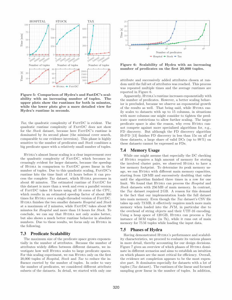
Figure 6: Scalability of Hydra with an increasingnumber of predicates on the first 20,000 tuples.
attribute and successively added attributes chosen at ran-dom until the full set of attributes was reached. This processwas repeated multiple times and the average runtimes arereported in Figure 6.Apparently, Hydra’s runtime increases exponentially with
the number of predicates. However, a better scaling behav-ior is precluded, because we observe an exponential growthof the results as well. That being said, while Hydra eas-ily scales to datasets with up to 15 columns, in situationswith more columns one might consider to tighten the pred-icate space restrictions to allow further scaling. The largerpredicate space is also the reason, why even Hydra can-not compete against more specialized algorithms for, e.g.,FD discovery. But although the FD discovery algorithmHyFD [13] finishes FD discovery in less than 15s on all ofthese datasets, a large share of valid DCs (up to 99%) onthese datasets cannot be expressed as FDs.
7.4 Memory UsageWhile one might assume that especially the DC checking
of Hydra requires a high amount of memory for storingthe involved cluster pairs, we observed Hydra to have alow memory footprint. To determine its peak memory us-age, we ran Hydra with different main memory capacities,starting from 128MB and successively doubling that valueuntil the algorithm finished three times in a row for onelimit. We found that Hydra can process the Hospital andStock datasets with 256MB of main memory. In contrast,the Tax dataset required 2GB. A reason for this demandis the fact that our implementation loads the full datasetinto main memory. Even though the Tax dataset’s CSV filetakes up only 73MB, it effectively requires much more mainmemory when loaded into the JVM, in particular due tothe overhead of string objects and their UTF-16 encoding.Using a heap space of 120GB, Hydra can process a Taxinstance of 50M tuples (in 7h), while it runs out of mainmemory for 75M tuples while loading the input data.
7.5 Phases of HydraHaving demonstrated Hydra’s performance and scalabil-
ity characteristics, we proceed to evaluate its various phasesin more detail, thereby accounting for our design decisions.Figure 7 gives an overview of which phases of Hydra domi-nate in different scenarios and aims to establish an intuitionon which phases are the most critical for efficiency. Overall,the evidence set completion appears to be the most expen-sive part. It dominates especially for datasets with a lot oftuples (Tax dataset). The runtimes of the linear and focusedsampling grow linear in the number of tuples. In addition,
320

0
5
10
15
20
25
250005000075000
100000
Number of tuples
Tim
e[s]
HOSPITAL
0
20
40
60
250005000075000
100000
Number of tuples
STOCK
0
500
1000
1500
2000
0
250000
500000
750000
1000000
Number of tuples
TAX
Random Sampling
Focused Sampling
Evidence Inversion
Minimization
Evidence Set Completion
Final Inversion
Figure 7: Runtime distribution for the differentphases of Hydra while scaling the number of tuples.
0
500
1000
0 50 100
150
Time [s]
Eviden
cesetsize
HOSPITAL
2000
4000
6000
0 50 100
150
Time [s]
STOCK
3000
6000
9000
0 50 100
150
Time [s]
TAX
Random Focused
Figure 8: Effectiveness of focused sampling. Theblack horizontal line marks the size of the completeevidence set. The random sampling serves here asa baseline.
the experiments on the Stock dataset with its 82 predicatesgive a notable impression of the influence of a high numberof predicates: in such circumstances the evidence inversionand the minimization take a much longer time than for data-sets with fewer predicates.
7.5.1 Sampling
In the following, the focused sampling’s effectiveness isevaluated w.r.t. its recall on Efull over time, as well as howthe specific sampling configurations influence the total run-time of Hydra. Note that although random and focusedsampling serve different purposes in Hydra, the randomsampling still can serve as a baseline to show how muchfaster Hydra’s focused sampling completes the evidence set.
Figure 8 evaluates the effectiveness of the focused sam-pling method described in Section 4. At different pointsin time, the size of the evidence set was measured up to atime limit of 150 seconds. The focused sampling methodachieves a much higher recall on the evidence set than therandom sampling methods in a short amount of time. Thisfact shows that our focused sampling is working well anddelivers a diversity of tuple pairs.
Figure 9 gives insight on the influence of Hydra’s twosampling parameters on Hydra’s total runtime: the numberof samples per tuple k in the random sampling and the effi-ciency threshold in the focused sampling phase. The overallresult of these experiments is thatHydra is relatively robustfor the choice of both parameters. Hydra performs a ran-dom sampling to estimate predicate selectivity. Figure 9a)shows the impact of different numbers of samples per tu-ple k for this phase: the runtime of the random sampling
0
10
20
30
10 20 30 40
Linear factor
Tim
e[s]
HOSPITAL
0
25
50
75
100
10 20 30 40
Linear factor
STOCK
0
1000
2000
10 20 30 40
Linear factor
TAXa)
0
10
20
30
1e-05
0.005 0.2
Threshold
Tim
e[s]
0
25
50
75
1e-05
0.005 0.2
Threshold
0
1000
2000
1e-05
0.005 0.2
Threshold
b)
Random Sampling
Focused Sampling
Evidence Inversion
Minimization
Evidence Set Completion
Final Inversion
Figure 9: Influence of a) the samples per tuple k inthe random sampling and of b) the focused sam-pling’s efficiency threshold on Hydra’s total run-time.
grows obviously linear with k, but due to better selectiv-ity estimations, the algorithm can save time in the evidencecompletion phase. The influence of this parameter choice issmall and 20 samples per tuple seem to work well for bothreal-world datasets and show only slight disadvantages forthe synthetic Tax dataset.In Figure 9b) we can observe the influence of the efficiency
threshold of the focused sampling with interesting results. Asmaller efficiency threshold causes more sampling iterationsand therefore of course a longer sampling phase. This in-crease does not come as a surprise, and on the Hospital andStock datasets the additional sampling pays off by reducingthe time spent on the evidence completion. For both data-sets the threshold 0.005 works best, and the performancedecreases in both directions (although only slowly). Unex-pectedly, for the Tax dataset a smaller threshold and, hence,more sampling, does not lower the time needed for the resultcompletion. One might think that this phenomenon occursbecause the tree of DCs that needs to be checked grows withan increasing sample. However, we could not measure a sub-stantial growth of the tree size. This suggests that due tothe more extensive sampling more complex predicate com-binations arise that need to be checked in the evidence setcompletion. Nevertheless, this observation is actually lessof a problem, because Hydra’s default threshold of 0.005for the sampling saves in this case on both, the time forthe sampling as well as the result completion. As the re-sult for the Tax dataset seems to constitute an exceptionand as it is also a generated dataset, the best threshold of0.005 observed on the other datasets was chosen for Hydra.Overall, Hydra is not very sensitive to the parameters andhence has proven its robustness.
7.5.2 Evidence Inversion
This experiment evaluates the gains of Hydra’s evidenceinversion in comparison to FastDC’s minimal cover search,which serves the same purpose. The underlying set cover
321

0.01
1.00
10 20 30
Number of predicates
Tim
e[s]
HOSPITAL
0.01
1.00
100.00
0 20 40 60 80
Number of predicates
STOCK
0.01
1.00
100.00
0 10 20 30 40 50
Number of predicates
TAX
FastDC FastDC-T Hydra
Figure 10: Scalability of different evidence inversionmethods with an increasing number of predicatescompared on the full evidence set (log-scale).
Table 3: Effect of different refiner weights on theruntime of the result completion.
Order criterion Hospital Stock Tax
Selectivity only 7.5s 422.8s > 2hFrequency / selectivity 6.1s 36.5s 38mFrequency only 81.6s > 2h > 2h
problem is NP-complete, so it is not surprising that Fig-ure 10 shows an exponential runtime behavior for both meth-ods with an increasing number of predicates (mind that they-axis for this graph is in log scale). However, as it is anNP-complete problem we should pay special attention anddesign the algorithm with great care as even a constant fac-tor speedup can have serious performance impacts. Thegeneral testing procedure is similar to that for the predicatescaling experiment with a time limit of 60 minutes. It isinteresting that FastDC’s cover inversion is faster if one ofits optimizations (the transitivity pruning rule) is disabled(FastDC-T ) and we therefore disabled it in general scalingexperiments. Nevertheless, Hydra’s evidence inversion isfaster by orders of magnitude in all scenarios. The observedspeedup is consistent with experiments in [12] for the do-main of functional dependency discovery: Fdep [6], whosecover inversion inspired that of Hydra, scales better withthe number of columns than FastFD [16], which in turninspired FastDC.
7.5.3 Evidence Set Completion
Hydra considers both the selectivity and the frequencyof partition refiners (predicates or pairs of predicates) to de-termine their order of evaluation in the evidence completionphase. Table 3 shows that it is indeed important to take theselectivity of the refiners into account as well as their fre-quency in the DC set. If only the selectivity is considered oronly the frequency, then the DC checking on the Tax datasetdoes not finish within a time limit of two hours. However, ifwe optimize the ratio of both, the checking finishes in about40 minutes. Additionally, we can see that the selectivity isa more important criterion than the frequency. If only thefrequency is taken into account the resulting runtimes areworse for every dataset compared to if only the selectivityis considered.
Finally, Figure 11 stresses the importance of minimizingthe set of DCs prior to checking them. The minimizationintroduces a small extra cost, but the total runtime can
be up to four times smaller than without the minimization(NOMIN ). The effect is bigger for datasets with a largernumber of predicates and therefore also a larger number ofDCs. The minimization not only reduces the number of DCsto be checked, but, as it also prefers smaller representations,the number of necessary refinement operations decrease aswell. In the same figure the effect of the pipelining (de-scribed in Section 6.2) on the runtime is shown by compar-ing Hydra to a version with disabled pipelining (NOPIPE).Although the pipelining’s effect on the runtime is negligible,it serves its purpose very well: it reduces the required mem-ory significantly. Without pipelining, Hospital can still beprocessed with 256MB of RAM, but for Stock the requiredmemory doubles (512MB) and Tax even requires four timesthe original amount (16GB instead of 2GB).
0.0
2.5
5.0
7.5
Hydr
a
NOPIPE
NOMIN
Tim
e[s]
HOSPITAL
0
100
200
300
400
Hydr
a
NOPIPE
NOMIN
STOCK
0
1000
2000
3000
4000
5000
Hydr
a
NOPIPE
NOMIN
TAX
Evidence Set Completion Minimization
Figure 11: Evaluation of variants for the result com-pletion comparing original Hydra with a version ofdisabled pipelining (NOPIPE) and no prior mini-mization (NOMIN ).
8. CONCLUSIONSWe presented the novel denial constraint discovery algo-
rithm Hydra. Hydra first approximates the set of validdenial constraints through intelligent sampling, and then ef-ficiently checks and corrects invalid results to finally obtaina complete and correct result, thereby avoiding to compareall tuple pairs in the given dataset. The algorithm’s ex-perimentally determined runtime grows only linearly in thenumber of tuples, and thus overcomes the quadratic runtimecomplexity of state-of-the-art DC discovery methods. Thisresults in a speedup by orders of magnitude, especially fordatasets with a large number of tuples. In fact, Hydra candeliver results in a matter of seconds that to date took hoursto compute.While Hydra discovers exact DCs, real-world data might
contain errors, so that an approximate version is a next step.An adapted version needs to count the number of times itsaw each evidence, ensuring not to count twice any evidenceoriginating from the same tuple pair. Due to the approx-imation, more evidences are necessary to preclude a DC.An adjusted efficiency definition in the focused samplingphase takes this into account and results in more sampling.Hydra’s cover inversion technique needs major changes toincorporate the observed frequency of evidences, while theevidence set completion requires almost no changes.
Acknowledgements. We thank the X. Chu, I. F. Ilyas,and P. Papotti for their help in starting this project. Thisresearch was partly funded by the German Research Society(grant no. FOR 1306).
322

9. REFERENCES[1] Z. Abedjan, L. Golab, and F. Naumann. Profiling
relational data: a survey. VLDB Journal,24(4):557–581, 2015.
[2] T. Bleifuß, S. Bulow, J. Frohnhofen, J. Risch,G. Wiese, S. Kruse, T. Papenbrock, and F. Naumann.Approximate Discovery of Functional Dependenciesfor Large Datasets. In Proceedings of the InternationalConference on Information and KnowledgeManagement (CIKM), pages 1803–1812, 2016.
[3] X. Chu, I. F. Ilyas, and P. Papotti. Discovering DenialConstraints. PVLDB, 6(13):1498–1509, 2013.
[4] X. Chu, I. F. Ilyas, and P. Papotti. Holistic DataCleaning: Putting Violations Into Context. InProceedings of the International Conference on DataEngineering (ICDE), pages 458–469, 2013.
[5] J. Ehrlich, M. Roick, L. Schulze, J. Zwiener,T. Papenbrock, and F. Naumann. Holistic dataprofiling: Simultaneous discovery of various metadata.In Proceedings of the International Conference onExtending Database Technology (EDBT), pages305–316, 2016.
[6] P. A. Flach and I. Savnik. Database dependencydiscovery: a machine learning approach. AICommunications, 12(3):139–160, 1999.
[7] F. Geerts, G. Mecca, P. Papotti, and D. Santoro. TheLLUNATIC data-cleaning framework. PVLDB,6(9):625–636, 2013.
[8] A. Heise, J.-A. Quiane-Ruiz, Z. Abedjan, A. Jentzsch,and F. Naumann. Scalable discovery of unique columncombinations. PVLDB, 7(4):301–312, 2013.
[9] Y. Huhtala, J. Karkkainen, P. Porkka, andH. Toivonen. TANE: An Efficient Algorithm forDiscovering Functional and Approximate
Dependencies. The Computer Journal, 42(2):100–111,1999.
[10] Z. Khayyat, W. Lucia, M. Singh, M. Ouzzani,P. Papotti, J.-A. Quiane-Ruiz, N. Tang, andP. Kalnis. Lightning Fast and Space EfficientInequality Joins. PVLDB, 8(13):2074–2085, 2016.
[11] T. Papenbrock, T. Bergmann, M. Finke, J. Zwiener,and F. Naumann. Data Profiling with Metanome.PVLDB, 8(12):1860–1863, 2015.
[12] T. Papenbrock, J. Ehrlich, J. Marten, T. Neubert,J.-P. Rudolph, M. Schonberg, J. Zwiener, andF. Naumann. Functional dependency discovery: Anexperimental evaluation of seven algorithms. PVLDB,8(10):1082–1093, 2015.
[13] T. Papenbrock and F. Naumann. A hybrid approachto functional dependency discovery. In Proceedings ofthe International Conference on Management of Data(SIGMOD), pages 821–833, 2016.
[14] Y. Sismanis, P. Brown, P. J. Haas, and B. Reinwald.Gordian: Efficient and scalable discovery of compositekeys. In Proceedings of the International Conferenceon Very Large Databases (VLDB), pages 691–702,2006.
[15] J. Szlichta, P. Godfrey, L. Golab, M. Kargar, andD. Srivastava. Effective and complete discovery oforder dependencies via set-based axiomatization.PVLDB, 10(7):721 – 732, 2017.
[16] C. Wyss, C. Giannella, and E. Robertson. FastFDs: Aheuristic-driven, depth-first algorithm for miningfunctional dependencies from relation instancesextended abstract. In Proceedings of the InternationalConference of Data Warehousing and KnowledgeDiscovery (DaWaK), pages 101–110, 2001.
323