eecs349 neural nets - computer science division ... pardo, northwestern university, machine learning...

Bryan Pardo, Northwestern University, Machine Learning EECS 349 Fall 2007

Machine Learning

Neural Networks


Biological Analogy

THE PERCEPTRON



Perceptrons

•  The “first wave” in neural networks •  Big in the 1960’s •  Marvin Minsky and Seymour Papert

– Perceptrons (1969)


A single perceptron

⎪⎩

⎪⎨⎧

>= ∑

=

else 0

0 if 10

n

iii xwσ

w1

w3

w2

w4

w5

x1

x2

x3

x4

x5

x0

w0

Inpu

ts Bias (x0 =1,always)


Logical Operators

⎪⎩

⎪⎨⎧

>= ∑

=

else 0

0 if 10

n

iii xwσ

-0.8 x0

0.5 x1

0.5 x2

AND

⎪⎩

⎪⎨⎧

>= ∑

=

else 0

0 if 10

n

iii xwσ

-0.3 x0

0.5 x1

0.5 x2

OR

⎪⎩

⎪⎨⎧

>= ∑

=

else 0

0 if 10

n

iii xwσ

1.0 x0

-1.0 x1

NOT


What weights make XOR?

•  No combination of weights works •  Linear combinations don’t allow this. •  No problem! Just combine perceptrons!

⎪⎩

⎪⎨⎧

>= ∑

=

else 0

0 if 10

n

iii xwσ

? x0

? x1

? x2


XOR

⎪⎩

⎪⎨⎧

>= ∑

=

else 0

0 if 10

n

iii xwσ

0 x0

0.6 x1

0.6 x2 ⎪⎩

⎪⎨⎧

>= ∑

=

else 0

0 if 10

n

iii xwσ

0 x0 ⎪⎩

⎪⎨⎧

>= ∑

=

else 0

0 if 10

n

iii xwσ

1 x0

XOR 1

1

-0.6

-0.6


The good news (so far)

•  We can make AND, OR and NOT •  Combining those let us make arbitrary

Boolean functions •  So…we’re good, right? •  Let’s talk about learning weights…


Learning Weights

•  Perceptron Training Rule •  Gradient Descent •  (other approaches: Genetic Algorithms)

⎪⎩

⎪⎨⎧

>= ∑

=

else 0

0 if 10

n

iii xwσ

? x0

? x1

? x2


Perceptron Training Rule

•  Weights modified for each example •  Update Rule:

The image cannot be displayed. Your computer may not have enough memory to open the image, or the image may have been corrupted. Restart your computer, and then open the file again. If the red x still appears, you may have to delete the image and then insert it again.


where

learning rate

target value

perceptron output

input value


Perceptron Training Rule

•  Converges to the correct classification IF – Cases are linearly separable – Learning rate is slow enough – Proved by Minsky and Papert in 1969

Killed widespread interest in perceptrons till the 80’s

WHY?


What’s wrong with perceptrons?

•  You can always plug multiple perceptrons together to calculate any function.

•  BUT…who decides what the weights are? – Assignment of error to parental inputs

becomes a problem…. – This is because of the threshold….

• Who contributed the error?


Problem: Assignment of error

⎪⎩

⎪⎨⎧

>= ∑

=

else 0

0 if 10

n

iii xwσ

? x0

? x1

? x2

Perceptron Threshold Step function

•  Hard to tell from the output who contributed what

•  Stymies multi-layer weight learning

LINEAR UNITS & DELTA RULE



Solution: Differentiable Function

∑=

=n

iii xw

0

σ

? x0

? x1

? x2

Simple linear function

•  Varying any input a little creates a perceptible change in the output

•  This lets us propagate error to prior nodes


Measuring error for linear units

•  Output Function

•  Error Measure:



data

target value

linear unit output


Gradient Decsent Rule •  To figure out how to change each weight to best

reduce error we take the derivative w.r.t that weight

•  …and then do some math-i-fication



The “delta” rule for weight updates ….YADA YADA YADA (this is in the book)

•  …and this gives our weight update rule

∑∈

−−≡∂

∂

Dddidd

i

xotwE ))(( ,


Learning Rate

Input on example


Delta rule vs. Perceptron rule

•  Perceptron Rule & Threshold Units – Learner converges on an answer ONLY IF

data is linearly separable – Can’t assign proper error to parent nodes

•  Delta Rule & Linear Units – Minimizes error even if examples are not

linearly separable – Linear units only make linear decision surfaces

(can’t make XOR even with many units)

THE MULTILAYER PERCEPTRON



A compromise function •  Perceptron

•  Linear

•  Sigmoid (Logistic)

⎪⎩

⎪⎨⎧

>= ∑

=

else 0

0 if 10

n

iii xwoutput

∑=

==n

iii xwnetoutput

0

output =σ (net) = 11+ e−net


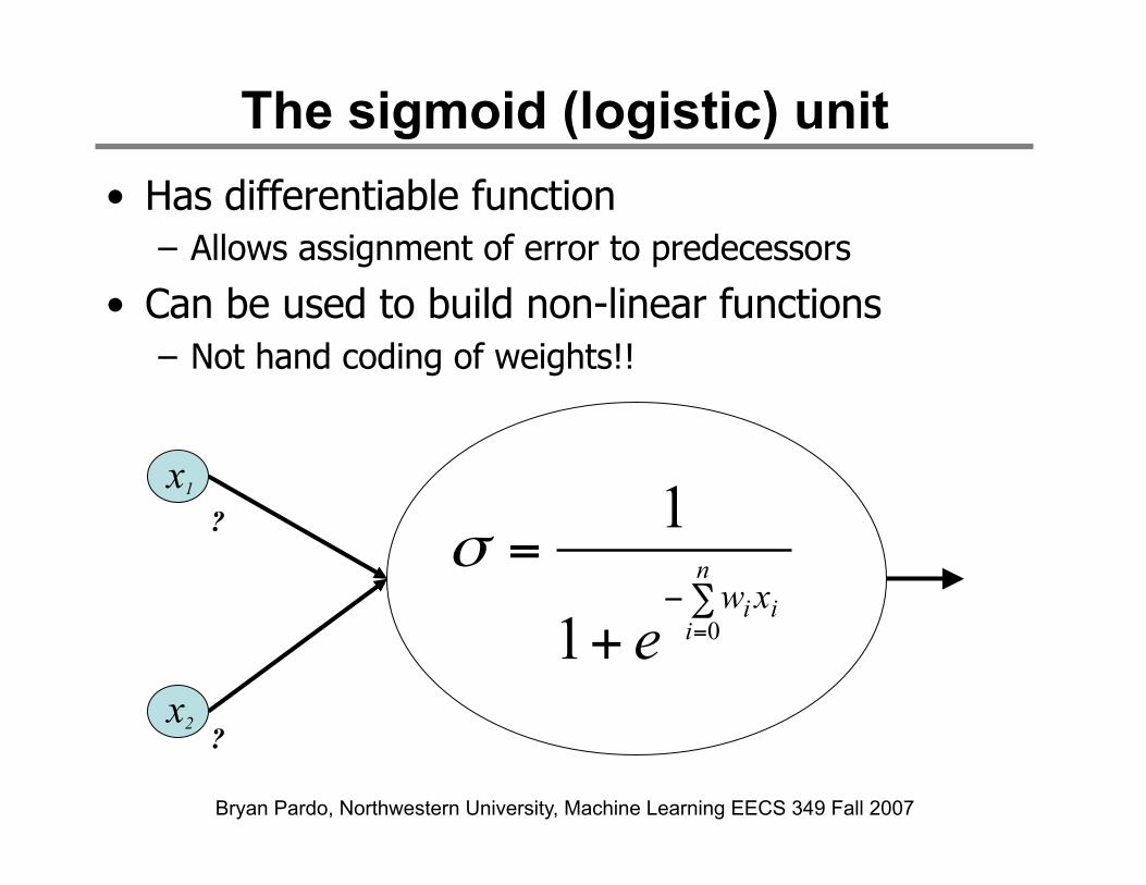
The sigmoid (logistic) unit •  Has differentiable function

–  Allows assignment of error to predecessors

•  Can be used to build non-linear functions –  Not hand coding of weights!!

? x1

? x2

∑−=+

= n

iii xw

e 01

1

σ


Differentiability is key!

•  Sigmoid is easy to differentiate

•  …so we basically make an elaborated version of the delta rule to handle learning weights

))(1()()(

yyyy

σσσ

−⋅=∂

∂


The Backpropagation Algorithm

jikjiji

ji

koutputsk

hkhhh

h

kkkkk

k

u

xδwww

δwooδδ

otooδδk

u ox

t,x

η+←

−←

−−←

∑∈

ight network weeach Update.4

)1( error term its calculate h,unit hidden each For .3

))(1( error term its calculate ,unit output each For 2.

network in the unit every for output thecompute andnetwork the to instanceInput 1.

example, ninginput traieach For


Logistic function

Coefficients

Output

Prediction

.5

.8

.4

0.6

“Probability of beingAlive”

∑−=+

= n

iii xw

e 01

1

σ

Inputs

Independent variables

Age 34

Gender

Stage 4

2 ∑


A very simple MLP

Inputs

Weights

Output

Independent variables

Dependent variable

Prediction

Age 34

Gender

Stage 4

.6

.5

.8

.2

.1

.3 .7

.2

Weights HiddenLayer

“Probability of beingAlive”

0.6 .4

.2 2

∑

∑ ∑

Output is a real number. Not categorical

How do you decide?

•  How to encode the data?

•  How many hidden nodes?

•  How many hidden layers? (just one, or MAYBE 2 for MLPs)

•  How big should each layer be?

•  How to encode/interpret the output?


Who is most similar?


•  Letters encoded as 10 by 10 pixel grids •  What if they are input to a single

perceptron unit? •  Would a multilayer perceptron do better? •  What pitfalls would you envision?

One possibility


INPUT LAYER HIDDEN LAYER OUTPUT LAYER

One input per pixel

One hidden node per potential shifted letter image

One output node per letter

a e i o

y u

Each node is connected to EVERY node in the prior layer (it is just too many lines to draw)

Rote memorization

•  Is the previous architecture different from rote memorization of cases?

•  Will it generalize?

•  What is the relationship between the size of the hidden layer and generalization?


Another possibility


INPUT LAYER HIDDEN LAYER OUTPUT LAYER

One input per pixel

small number of nodes: 1 per important feature

One output node per letter

a e i o

y u

Each node is connected to EVERY node in the prior layer (it is just too many lines to draw)

Interpreting the output

•  Treat it as a confidence/probability?

•  Force it to 0 or 1 to be a decision?

•  Quantize to a range of values?

•  How about different output architectures?



Multi-Layer Perceptrons are

•  Models that resemble nonlinear regression

•  Also useful to model nonlinearly separable spaces

•  Can learn arbitrary Boolean functions

•  Use gradient descent and are thus susceptible to being stuck in local minima

•  Opaque (internal representations are not interpretable)

HEBBIAN LEARNING



Donald Hebb

•  A cognitive psychologist active mid 20th century

•  Influential book: The Organization of Behavior (1949)

•  Hebb’s postulate "Let us assume that the persistence or repetition of a reverberatory activity (or "trace") tends to induce lasting cellular changes that add to its stability.… When an axon of cell A is near enough to excite a cell B and repeatedly or persistently takes part in firing it, some growth process or metabolic change takes place in one or both cells such that A's efficiency, as one of the cells firing B, is increased.


Pithy version of Hebb’s postulate

Cells that fire together, wire together.

HOPFIELD NETWORKS



Hopfield nets are

•  “Hebbian” in their learning approach •  Fast to train •  Slower to use •  Weights are symmetric •  All nodes are input & output nodes •  Use binary (1, -1) inputs and output •  Used as

Associative memory (image cleanup) Classifier

Using a Hopfield Net 10 by 10 Training patterns


Query pattern (to clean or classify) Output pattern

Fully connected 100 node network

(too complex to draw)


Training a Hopfield Net •  Assign connection weights as follows

wij =xc, i xc, j if i ≠ j

c=1

C

∑0 if i = j

⎧

⎨⎪

⎩⎪

c index number for C many class exemplarsi, j index numbers for nodeswi, j connection weight from node i to node jxc, i ∈{+1,−1} element i of the exemplar for class c


UPDATED (again. 3rd time’s the charm) Using a Hopfield Net

Force output to match an unknown input pattern

Iterate the following function until convergence

Note: this means you have to pick an order for updating nodes. People often update all the nodes in random order

si (0) = xi ∀i

si (t +1) =1 if 0 ≤ wijsj (t)

j=1

N

∑

−1 else

$

%&

'&

Here, si (t) is the state of node i at time tand xi is the value of the input pattern at node i


Using a Hopfield Net Once it has converged… FOR INPUT CLEANUP: You’re done. Look at the final state of the network. FOR CLASSIFICATION: Compare the final state of the network to each of your input examples. Classify it as the one it matches best.

Input Training Examples

Image from:R. Lippman, An Introduction to Computing with Neural Nets, IEEE ASSP Magazine, April 1987

Why isn’t 5 in the set of examples?

Output of network over 8 iterations

Image from:R. Lippman, An Introduction to Computing with Neural Nets, IEEE ASSP Magazine, April 1987

Input pattern After 3 iterations

After 7 iterations

First iteration

Characterizing “Energy”

Image from: http://en.wikipedia.org/wiki/Hopfield_network#mediaviewer/File:Energy_landscape.png

•  As is updated, the state of the system converges on an “attractor”, where

•  Convergence is measured with this “Energy” function: si (t +1) = si (t)

si (t)

E(t) = − 12

wiji, j∑ si (t)s j (t)

Note: people often add a “bias” term to this function. I’m assuming we’ve added an extra “always on” node to make our “bias”

Limits of Hopfield Networks

•  Input patterns become confused if they overlap

•  The number of patterns it can store is about 0.15 times the number of nodes

•  Retrieval can be slow, if there are a lot of nodes (it can take thousands of updates to converge)


RESTRICTED BOLTZMAN MACHINE (RBM)


About RBNs

•  Related to Hopfield nets

•  Used extensively in Deep Belief Networks

•  You can’t understand DBNs without understanding these


Standard RBM Architecture

2 layers (hidden & input) of Boolean nodes Nodes only connected to the other layer


xixi xi xi xi

Hidden Units

Input Units

Weight Matrix



xixi xi xi xi

Hidden Units

Input Units

Weight Matrix

•  Setting the hidden nodes to a vector of

values updates the visible nodes…and vice versa



xixi xi xi xi

•  Setting the hidden nodes to a vector of

values updates the visible nodes…and vice versa

Contrastive Divergence Training


1.  Pick a training example. 2.  Set the input nodes to the values given by the example. 3.  See what activations this gives the hidden nodes. 4.  Set the hidden nodes at the values from step 3. 5.  Set the input node values, given the hidden nodes 6.  Compare the input node values from step 5 to the the

input node values from step 2 7.  Update the connection weights to decrease the

difference found in step 6. 8.  If that difference falls below some epsilon, quit.

Otherwise, go to step 1.

DEEP BELIEF NETWORK (DBN)


What is a Deep Belief Network?

•  A stack of RBNS

•  Trained bottom to top with Contrastive Divergence

•  Trained AGAIN with supervised training (similar to backprop in MLPs)


xi

W1

W2

W3

W4

x

h1

h2

h3

RBN

What is a Deep Belief Network?

•  A stack of RBNS

•  Trained bottom to top with Contrastive Divergence

•  Trained AGAIN with supervised training (similar to backprop in MLPs)


xi

W1

W2

W3

W4

x

h1

h2

h3RBN

Why are DBNs important?

•  They are state-of-the-art systems for doing certain recognition tasks – Handwritten digits – Phonemes

•  They are very “hot” right now

•  They have a good marketing campaign “Deep learning” vs “shallow learning”


How does “deep” help?

•  It may be possible to much more naturally encode problems like the parity problem with deep representations than with shallow ones


Why not use standard MLP training?

•  Fading signal from backprop

•  The more complex the network, the more likely there are local minima

•  Memorization issues

•  Training set size and time to learn


Benefits

•  Seems to allow really deep networks (e.g. 10 layers)

•  Creating networks that work better than anything else out there for some problems (e.g. digit recognition, phoneme recognition)

•  Lets us again fantasize about how we’ll soon have robot butlers with positronic brains.


The promise of many layers

•  Each layer learns an abstraction of its input representation (we hope)

•  As we go up the layers, representations become increasingly abstract

•  The hope is that the intermediate abstractions facilitate learning functions that require non-local connections in the input space (recognizing rotated & translated digits in images, for example)


BIG BIG data

•  DBNs are often used in the context of millions of training steps and millions of training examples


RECURRENT NETS


Read up on your own

•  Things like multi-layer perceptrons are feed-forward

•  Boltzman machines and Hopfield networks are bidirectional

•  These have one-way links, but there are loops

•  You’ll have to read up on your own


SPIKE TRAIN NETS


Read up on your own

•  These are attempts to actually model neuron firing patterns

•  There is no good learning rule •  There is no time to talk about these


CONVOLUTIONAL NETS


Read up on your own

•  Another type of deep network •  References to this work in the course

readings


eecs349 neural nets - computer science division ... pardo, northwestern university, machine learning...

Documents