EEB Climate Module

Day 3: 2/16/11

Lecture Outline

• Part I: Paleoclimate & Reanalysis Data

– Proxies

– Reanalysis Models

• Part II: Regional Climate Models

– Downscaling

– Organizations & Projects

PALEOCLIMATE & REANALYSISPart I

Earth

• The formation of our solar system is thought to have been triggered by shockwaves (a big bang?) from +1 nearby supernovae (4-6 billion yrs BP).

• The primordial atmosphere of Earth had been removed through collision of large solar objects &/or swept away by intense solar winds from a young Sun (a G2V star).

• The 2nd atmosphere of Earth was gasses trapped in the molten surface of the young Earth released through out-gassing.– Due to the distance from the sun & composition of the 2nd

atmosphere, the temperature of H2O could remain at it’s triple point.• Liquid H2O formed vast oceans, & the atmosphere was composed

mainly of nitrogen.

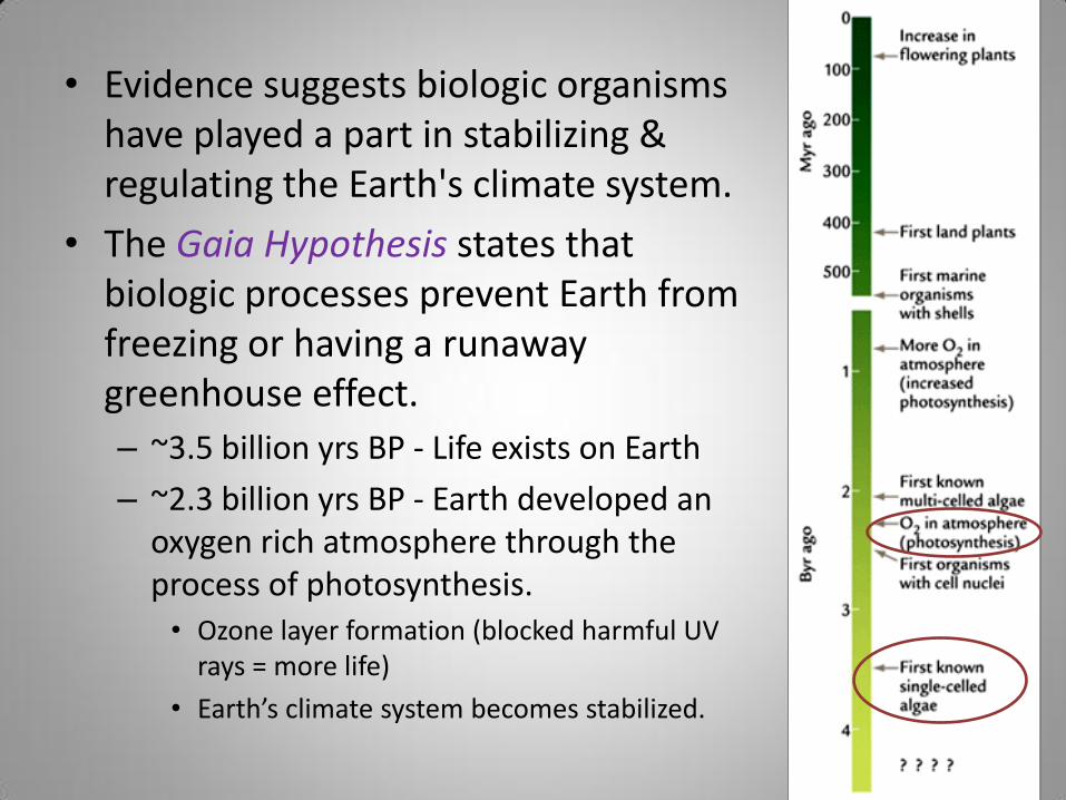
• Evidence suggests biologic organisms have played a part in stabilizing & regulating the Earth's climate system.

• The Gaia Hypothesis states that biologic processes prevent Earth from freezing or having a runaway greenhouse effect.

– ~3.5 billion yrs BP - Life exists on Earth

– ~2.3 billion yrs BP - Earth developed an oxygen rich atmosphere through the process of photosynthesis.• Ozone layer formation (blocked harmful UV

rays = more life)

• Earth’s climate system becomes stabilized.

Natural Climate Forcing

• Natural Climate Forcing (3 main methods):

– Variations in solar outputs

• Atmospheric composition changes

• Sun spots

– Changes in Earth’s orbit

• Milankovitch Cycles

– Plate tectonics

• Movement of land masses

• Volcanic activity changes

Proxies

• Proxy data - gathered from natural recorders of climate variability. – Tree rings, ice cores, fossil pollen, ocean sediments, coral, &

historical data (ship & local data, unconventional written records).

– Extends understanding of past climate beyond the ~140 yr instrumental record.

– Allows for study of natural climate variability & anthropogenically-induced climate change.

• Paleoclimatology - the study of past climate prior to instrumental record. – Instrumental records of climate are limited to the last ~100

yrs.• Not enough data to assess long-term trends & forcings.

Source: TAR, WG1

Types of Proxy Data

• Paleoclimate researchers conduct studies on:– Boreholes:

• Ice cores

• Sediment from oceans & lakes– Varves

• Pollen records

– Coral cores

– Tree rings

– Other – snail shells, fossilized excrement, pack rat middens, etc.

• Most proxies use methods of isotope dating.

Proxy TypeSampling Interval (min.)

Temporal Scope

(order: yr) Temp.

Precip.or waterbalance

Chemical comp.(air or water)

Biomass or

vegetation

Volcanic eruptions

Sea Level

Solar Activity

Historical Records

day/hr ~103 Yes Yes Yes Yes Yes Yes Yes

Tree Rings yr/season ~104 Yes Yes NO Yes Yes NO Yes

Lake Sediments

yr to 20 yr ~104~106 Yes Yes NO Yes Yes NO NO

Corals yr ~104 Yes Yes Yes NO NO Yes NO

Ice Cores yr ~5 X 105 Yes Yes Yes Yes Yes NO Yes

Pollen 20 yr ~105 Yes Yes NO Yes NO NO NO

Speleothems 100yr ~5 X 105 Yes Yes Yes NO NO NO NO

Loess 100yr ~106 NO Yes NO Yes NO NO NO

Geomorphic features

100 yr ~106 Yes Yes NO NO Yes Yes NO

Marine sediments

500 yr ~107 Yes Yes Yes Yes Yes Yes NO

Organizations

• NOAA’s World Data Center for Paleoclimatology– http://www.ncdc.noaa.gov/paleo/paleo.html

• Neotoma Paleoecology Database - multiproxy database that includes fossil data for the past 5 million years.– www.neotomadb.org

– Created by PSU• 0-5 million yrs BP.

• Paleoclimate Model Intercomparison Project Phase 2 (PMIP2)– http://pmip2.lsce.ipsl.fr/

– Created by LSCE• 0- 21,000 yrs BP.

Isotope Dating• Isotopes - atoms that contain the same # of protons

(=atomic #) but a different # of neutrons (atomic mass is different).– Created through cosmic ray/particle interaction.

• Creation reliant on solar/cosmic activity.

– Some isotopes are radioactive/unstable.

• Radioactive decay – process where emission of radiation or a particle occurs in the nucleus, alters the total number of nucleons (protons & neutrons) in the nucleus.– Parent (unstable isotope) Daughter (decay product isotope).– Radioactive decay begins after formation.

• Based on decay rate & the isotope ratio, date of isotope (layer in which the isotope is buried) can be determined.

– 4 types of radioactive decay.– If isotope ratio is very small, age of layer is very old.– Radioactive decay is the “clock in a rock.”

Examples

• Ex. U-238 decays to Pb-206; U-235 decays to Pb-207.– This is was used to construct the age of the Earth to be

approx 4.5ish billion yrs old.• Isochron dating – decay products can be stable &/or unstable.

– Pb-207 & Pb-206 additionally decay to Pb-2004.

• Ex. Carbon-14 is created in atmosphere from atmospheric Nitrogen interaction with solar particles. – C-14 undergoes ‘beta-decay’, loss of electron & gain of

proton, & becomes N-14.

– If ratio of C-14 to normal carbon is low = object is old

N14

1. Cosmic Ray/Particle

2. Atom (??)

3. Neutron (maybe)

3. Proton (maybe)

C14

4. Added neutron (neutron capture) dislodges a proton

5. Proton5. Unstable C-14 (6 protons, 8 neutrons)

6. Tree takes in C-14 & C-12 (C-14/C-12 = 1ish)

7. Tree dies, sedimentary layer contains tree remains.• C-14 decays at a fixed

rate in sediment = N-14 + electron.

• Sediment core is taken.• C-14/C-12 =

0.000000001

Stable Isotopes

• Isotopes of an element often exist naturally & are relatively stable.– The ratio of nuclides found in geologic strata can be

used to reconstruct past climate & atmospheric composition.

• Oxygen has 3 main isotopes: O-16 (99.76%), O-17 (0.03%), & O-18 (0.19%).– The ratio of O-18 to O-16 in ice & deep sea cores is

temperature dependent.• High ratio in aquatic plankton = cold period

• High ratio in land biota = warm period

Boreholes

• Boreholes are cores drilled into the Earth crust. • Can be used to obtain ice, pollen, sediment, etc.

cores.• Borehole data can also be used to examine

surface temperatures.– The geothermal gradient is used to examine changes

in past surface temperatures.• As heat is transferred downward there are indications of

warming or cooling of strata.

• PBS NOVA Antartic Ice Core clip (start at 16:00, end at 27:00)

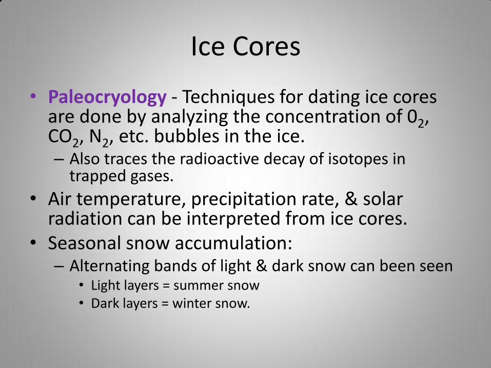
Ice Cores

• Paleocryology - Techniques for dating ice cores are done by analyzing the concentration of 02, CO2, N2, etc. bubbles in the ice.– Also traces the radioactive decay of isotopes in

trapped gases.

• Air temperature, precipitation rate, & solar radiation can be interpreted from ice cores.

• Seasonal snow accumulation:– Alternating bands of light & dark snow can been seen

• Light layers = summer snow• Dark layers = winter snow.

Lake Sediment

• Paleolimnology - the study of past conditions of inland fresh water bodies.

• Measurements from lake & bog sediment core are used to indicate past water temp, physical properties, biology, & chemistry.

– Lake ecosystems respond to climate change in many ways.

– Data from sediments can be used to reconstruct climate.

Pollen Sediment

• Paleopalynology

– Palynology – the study of palynomorphs, like pollen, spore, etc.

• Pollen grains which are washed or blown into lakes can accumulate in sediments & provide a record of past vegetation.

– Different types of pollen in lake sediments reflect the vegetation that was present around the lake.

• Climate conditions are inferred from vegetation.

Corals

• Coral core data consists of isotope & trace metal analyses from corals located around the globe. – Corals serve as proxies of upper ocean environment, such

as SST & salinity.– Coral structure is examined through: Growth rates, annual

skeletal banding, the longevity of individual colonies.• Growth rings

• Coral skeletons are suitable for high-res radioactive dating.

• Geochemical climate proxies can be applied to coral aragonite.– Produce ~ monthly resolution records back into the late

Quaternary.

Tree Rings

• Dendroclimatology - study of the annual growth tree rings & the assembling of continuous chronologies of climate conditions.

• Offers a high res (seasonal or annual) form of paleoclimate reconstruction for most of the Holocene.

• Trees interact directly with the microenvironment of the leaf & root surfaces. – Growth may be affected by many aspects of the

microclimate: sunshine, precipitation, temperature, wind speed, & humidity .• Climate extremes & hazards (fire & drought) can also be inferred.

– Non-climatic factors also affect tree rings.• Competition, defoliators, & soil nutrient characteristics.

Institute of Plant and Animal Ecology

Summer temperature anomalies for the past 7,000 yrs from tree rings.

Climate Reanalysis Models

• Important for monitoring past climate variability & trends. – Provides a comprehensive spatial & temporal depiction of

the state of the climate system– Improves seasonal prediction & validation activities. – Fills in ‘gaps’ where obs have been sparse in time/space.

• A reanalysis dataset typically extends over several decades or longer.

• Usually global coverage as well as 4-dimensional (x,y,z,t) coverage.– Resolution varies by model.

• Resolution usually finer than GCMs.

Running a Reanalysis Model

• Models are based on well-established physical relationships.

• Obs are assimilated ("input") into the climate model throughout the entire reanalysis period in order to reduce the affects of modeling changes on climate statistics. – Reduces the effects of model bias.– Obs are from many sources:

• Ships, satellites, ground stations, radiosondes, & radar.

– In areas of less obs, less confidence in model output.

• NOAA’s ESRL PSD url: http://www.esrl.noaa.gov/psd/data/gridded/reanalysis/

• Reanalysis Intercomparison and Observations (RIO) url: http://reanalyses.org/

• 20th Century Reanalysis Project Clip (Sep. 2010)

REGIONAL CLIMATE MODELPart I

The Resolution Problem

• For adaptation purposes, there is a clear need for finer resolution AOGCM output.– Most AOGCMs (from AR4) have resolutions of ~2o

x ~2o.

– For finer AOGCM resolution, computational power, biases, & parameterization problems must be addressed.

• Regional Climate Models (RCMs) are created to examine an area of interest at much finer-scales.

Types of RCM

• Stretched-Grid Global Climate Model (SGCM)

– Provides the global/continuous coverage of a GCM, but with variable-resolution gridding.

• SGCMs contract the global grid to focus on 1 area of interest.

– Multiple runs can be done with any GCM.

– Stretched Grid Model Intercomparision Project (SGMIP):

• http://essic.umd.edu/~foxrab/sgmip.html

Cont…

• Downscaled Climate Model

– Downscaling – methods of refining resolution.

• Using low resolution data to acquire high resolution data.

– 2 main downscaling techniques:

• Statistical

• Dynamical– Limited Area Models (LAM)

Statistical Downscaling

• Based on the numerical physical relationships among weather/climate variables.– Relationships between obs & large scale GCM variables.

• Topology is needed.

• Stationarity assumption - Assumes relationships do not change.

• The affect of adjacent cells is not included.

• Resolution of SD RCMs are as fine as the point physical relationships allow.– Generally doesn’t need a lot of computational power.

• Ed Mauer’s SD RCM for the US:– http://www.engr.scu.edu/~emaurer/data.shtml

• Monthly, 1/8 degree resolution.

GCM grid cell output

Point on surface of Earth:-Topography & features-Equations to represent phys. processes

SD RCM grid cell output

Dynamical Downscaling• High resolution LAM nested w/i an AOGCM.

– Parameterization may be the same in both models.– Parameterization may be region-specific or geographically

‘tuned’.• CORDEX project

• Initial conditions & boundary conditions are from AOGCM.– Boundary condition weighting is done for RCM cells– DD RCM & AOGCM are not run at same time steps.

• Time steps must match grid spacing– Ex. 10 km resolution = ~30 sec; 250 km resolution = 20 minute

• Resolution & size of LAM will determine computational power needed (supercomputer is needed).

• Multi-Model Ensembles of DD RCMs:– PRUDENCE & ENSEMBLES (Europe)– NARCCAP (US)

GCM – continuous, global data

LAM

Caveat of RCMs

• NO studies clearly demonstrate that RCMs produce superior estimation of impacts or better adaptation measure than GCMs.– RCMs use boundary conditions from GCMs (which

have bias).• RCMs also have biases.

– Are the biases doubled?

– Some RCM are site-specific, & should not apply to other regions (WCRP CORDEX project)

• GCMs are being run at high resolutions for AR5 & for time-slice experiments.– Multiple versions of a model are also being run.

Time-Slice Experiments

• In timeslice experiments, the atmospheric component of an AOGCM is run without the full coupled ocean component of the model. – Boundary conditions for sea surface & ice for the historical run

are based on obs data.– Boundary conditions for the projected run are derived by

perturbing observed sea-surface temperature & ice data by an amount based on the results of the full AOGCM.

• It's called a 'timeslice' experiment because it only simulates certain slices of time.– ~30 years

• Computational requirements of the simulation are much lower = model can be run at a higher resolution.

The North American Regional Climate Change Assessment Program (NARCCAP)

• NARCCAP -international program to produce high-res simulations in order to investigate uncertainties in regional scale climate projections for use in impacts research.

• 6 RCMs (with 4 AOGCMs) are run for the US & most of Canada.– Use the SRES A2 for the 21st century (2041-2070).

• Simulations were also produced for the current (historical) period using NCEP Reanalysis II data for the period 1979-2004.

Phase I Phase II

NCEP GFDL CGCM3 HADCM3 CCSM

CRCM X X X

ECPC X X X

HRM3 X X X

MM51 X X X

RCM3 X X X

WRFP X X X

Model Projection

CRCM Polar Stereographic

ECPC Polar Stereographic

HRM3 Rotated Pole

MM5I Lambert Conformal

RCM3 Transverse Mercator

WRFP Lambert Conformal

•All the RCMs are run at a spatial resolution of 50 km.•Also includes 2 timeslice experiments at 50 km resolution using the GFDL atmospheric model (AM2.1) & the NCAR CCSM atmospheric model (CAM3).

End Lecture Portion

Begin Exercise