EE513Audio Signals and Systems

Statistical Pattern Classification

Kevin D. DonohueElectrical and Computer Engineering

University of Kentucky

Interpretation of Auditory Scenes Human perception and cognition greatly exceeds any

computer-based system for abstracting sounds into objects and creating meaningful auditory scenes. This perception of objects (not just detecting acoustic energy) allows for interpretation of situations leading to an appropriate response or further analyses. Sensory organs (ears) separate acoustic energy into frequency bands

and convert band energy into neural firings The auditory cortex receives the neural responses and abstracts an

auditory scene.

Auditory Scene Perception derives a useful representation of reality from

sensory input. Auditory Stream refers to a perceptual unit associated with

a single happening (A.S. Bregman, 1990) .

Acoustic to Neural

Conversion

Organize into Auditory Streams

Representation of Reality

Computer Interpretation In order for a computer algorithm to interpret a scene

Acoustic signals must be converted to numbers using meaningful models. Sets of numbers (or patterns) are mapped into events (perceptions). Events are analyzed with other events in relation to the goal of the

algorithm and mapped into a situation (cognition or deriving meaning). Situation is mapped into an action/response.

Numbers extracted from the acoustic signal for the purpose of classification (determination of event) are referred to as features. Time -based features are extracted from signal transforms such as:

Envelope Correlations

Frequency-based features are extracted from signal transforms such as: Spectrum (Cepstrum) Power Spectral Density

Feature Selection Example Consider a problem of discriminating between the spoken

words yes and no based on 2 features:1. The estimate of first formant frequency g1 (resonance of the

spectral envelope)

2. The ratio in dB of the amplitude of the second formant frequency over the third formant frequency g2.

A fictitious experiment was performed and these 2 features were computed for 25 recordings of people saying these words. The feature were plotted for each class to develop an algorithm to classify these samples correctly.

Feature Plot Define a feature

vector.

Plot G, given a yes was spoken, with green o’s, and given a no was spoken, be wiht red x’s.

2

1

gg

G

440 460 480 500 520 540 560 580 600-10

-5

0

5

10

15

20

First Formant Frequency ( g1 )

dB

of R

atio

Fo

rma

nt 3

ove

r 4

( g

2 )

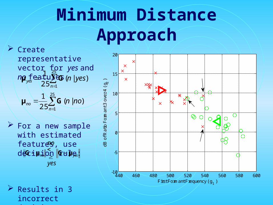
Minimum Distance Approach Create representative

vector for yes and no features

For a new sample with estimated features, use decision rule:

Results in 3 incorrect decisions.

25

1

)|(25

1

nyes yesnGμ

25

1

)|(25

1

nno nonGμ

yesno

yes

no

μGμG

440 460 480 500 520 540 560 580 600-10

-5

0

5

10

15

20

First Formant Frequency ( g1 )

dB

of R

atio

Fo

rma

nt 3

ove

r 4

( g

2 )

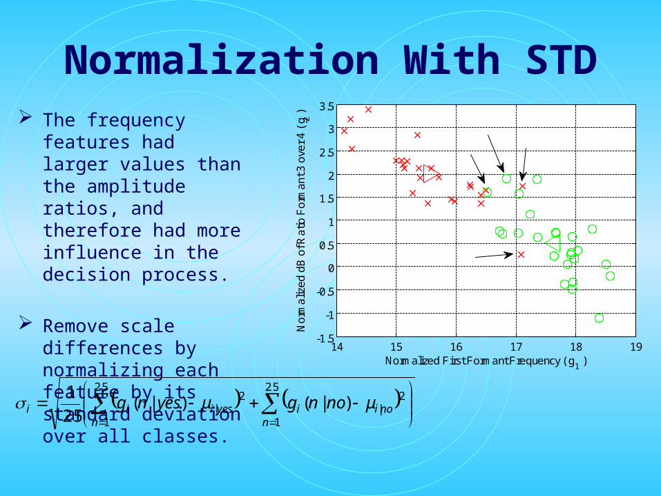
Normalization With STD The frequency features

had larger values than the amplitude ratios, and therefore had more influence in the decision process.

Remove scale differences by normalizing each feature by its standard deviation over all classes.

Now 4 errors result (why would it change?)

25

1

25

1

2|

2| )|()|(

25

1

n nnoiiyesiii μnongμyesng

14 15 16 17 18 19-1.5

-1

-0.5

0

0.5

1

1.5

2

2.5

3

3.5

Normalized First Formant Frequency ( g1 )

No

rma

lize

d d

B o

f Ra

tio F

orm

an

t 3 o

ver

4 (

g 2 )

Minimum Distance Classifier Consider feature vector x with the potential to be classified as

belonging to K exclusive classes. Classification decision will be based on the distance of the

feature vector to one of the template vectors representing each of the K classes.

The decision rule is for a given observation x and set of template vectors zk for each class, decide on class k such that:

)()(minarg kT

kk

k

D zxzx

Minimum Distance Classifier If some features need to be weighted more than others in the decision

process, as well as exploiting correlation between the features, the distance for each feature can be weighted to result in the weighted minimum distance classifier:

where W is a square matrix of weights with dimension equal to length of x. If W is a diagonal matrix, it simply scales each of the features in the decision process. Off diagonal terms scale the correlation between features. If W is the inverse of the covariance matrix of the features in x, and zk is the mean feature vector for each class, then the above distances are referred to as the Mahanalobis distance.

)()(minarg kT

kk

k

D zxWzx

1

1E

1 E

K

k

Tkkk k

Kk zxzxWxz

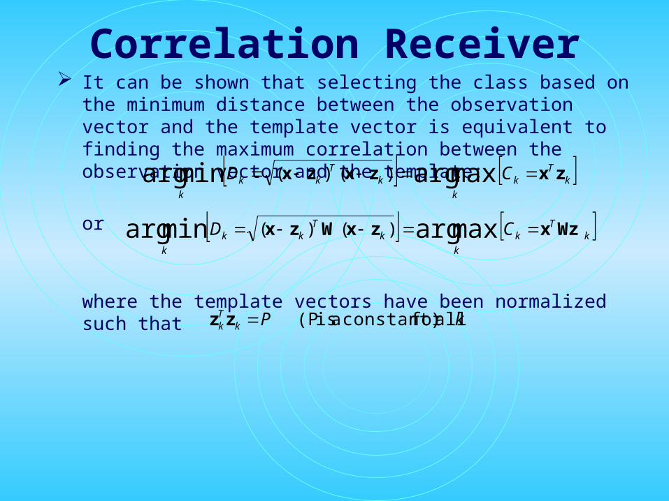
Correlation Receiver It can be shown that selecting the class based on the minimum distance

between the observation vector and the template vector is equivalent to finding the maximum correlation between the observation vector and the template:

or

where the template vectors have been normalized such that

kT

k

k

kT

kk

k

CD zxzxzx maxargminarg )()(

kPkTk allfor constant) a is (P zz

kT

k

k

kT

kk

k

CD WzxzxWzx maxargminarg )()(

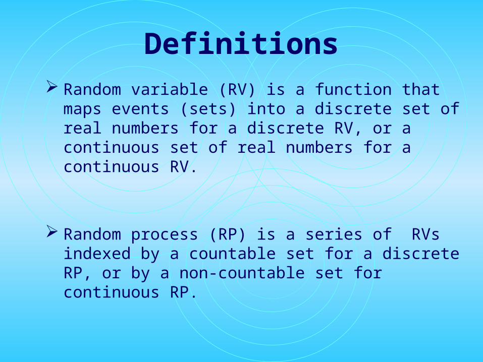
Definitions Random variable (RV) is a function that maps events (sets)

into a discrete set of real numbers for a discrete RV, or a continuous set of real numbers for a continuous RV.

Random process (RP) is a series of RVs indexed by a countable set for a discrete RP, or by a non-countable set for continuous RP.

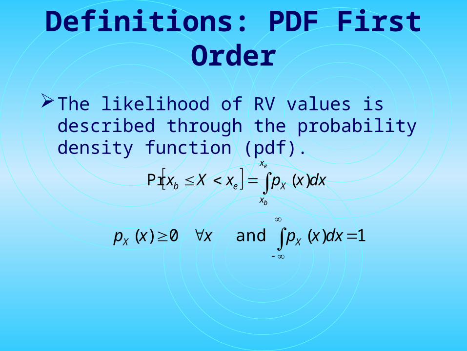
Definitions: PDF First Order

The likelihood of RV values is described through the probability density function (pdf).

e

b

x

x

Xeb dxxpxXx )(Pr

1)( and 0)(

dxxpxxp XX

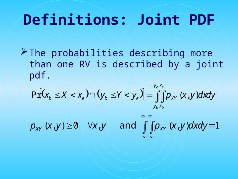
Definitions: Joint PDF

The probabilities describing more than one RV is described by a joint pdf.

e

b

e

b

y

y

x

x

XYebeb dydxyxpyYyxXx ),(Pr

1),( and , 0),(

dxdyyxpyxyxp XYXY

Definitions: Conditional PDF

The probabilities describing a RV given that the another event has already occurred is described by a conditional pdf.

Closely related to this is Bayes’ rule:

)(

),()|(| yp

yxpyxp

Y

XYYX

)(

)()|()|(

)()|(),()()|(

||

||

xp

ypyxpxyp

xpxypyxpypyxp

X

YYXXY

XXYXYYYX

Examples: Gaussian PDF A first order Gaussian RV pdf (scalar x) with mean µ and

standard deviation is given by:

A higher order joint Gaussian pdf (column vector x) with mean vector m and covariance matrix is given by:

2

2

2 2

)(exp

2

1)(

x

xpX

T

Tn

T

n

xxx

p

))((E

E

,,

)()(2

1exp

2

1)(

21

12/12/X

mxmx

xm

x

mxmxx

Example Uncorrelated

Prove that for an Nth order sequence of uncorrelated Gaussian zero-mean RVs the joint PDF can be written as:

Note that for Gaussian RVs uncorrelated implies statistical independence.Assume variances are equal for all elements. What would the autocorrelation of this sequence look like?How would the above analysis change if RVs were not zero mean?

N

i i

i

i

X

xp

12

2

2 2

)(exp

2

1)(

x

Class PDFsWhen features are modeled as RVs, their pdfs can be used to derive distance measures for the classifier, and an optimal decision rule that minimizes classification error can be designed.

Consider K classes individually denoted by k. Feature values associated with each class can be described by:

a posteriori probability (likelihood the class after observation/data)

a priori probability (likelihood the class before observation/data)

Likelihood function (likelihood observation/data given a class)

)( xkkp

)( kp xx

)( kkp

Class PDFsThe likelihood function can be estimated through empirical studies. Consider 3 speakers whose 3rd formant frequency is distributed by:

Classifier probabilities can be obtained from Bayes’ rule

)(

)()()(

xp

pxpxp

x

kkkxkk

-8 -6 -4 -2 0 2 40

0.2

0.4

0.6

0.8

1

Feature Value

1 (-3,.9)

2 (0, 1.2)

3 (2, .5)

Decision Thresholds

)( 1xpx

)( 2xpx

)( 3xpx

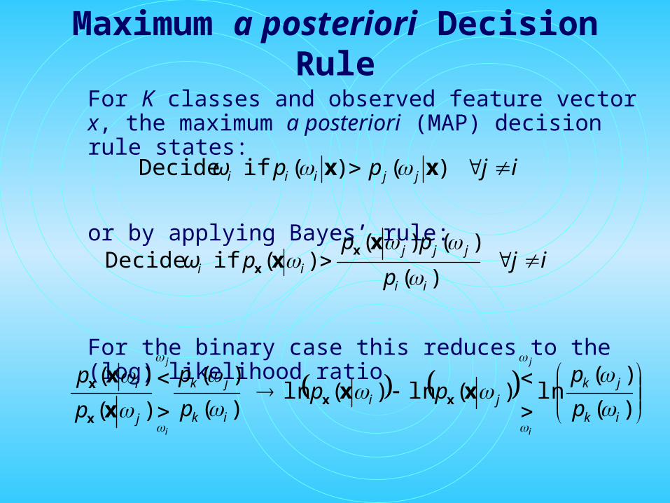
Maximum a posteriori Decision Rule

For K classes and observed feature vector x, the maximum a posteriori (MAP) decision rule states:

or by applying Bayes’ rule:

For the binary case this reduces to the (log) likelihood ratio

ijppω jjiii )()( if Decide xx

ijp

pppω

ii

jjj

ii )(

)()()( if Decide

x

xx

x

)(

)(ln)(ln)(ln

)(

)(

)(

)(

ik

jkji

ik

jk

j

i

p

ppp

p

p

p

p

i

j

i

j

xxx

xxx

x

x

ExampleConsider a 2 class problem with Gaussian distributed feature vectors

Derive the log likelihood ratio and describe how the classifier uses distance information to discriminate between the classes.

See related link: http://en.wikipedia.org/wiki/Linear_discriminant_analysis

2222

1111

2211

21

))((E

))((E

E E

,,

T

T

TNxxx

mxmx

mxmx

xmxm

x

HomeworkConsider a 2 features for use in a binary classification problem. The features are Gaussian distributed are form feature vectorx = [x1, x2]T. Derive the log likelihood ratio and corresponding classifier for the 3 different cases listed below:•1) 2)

3) 4)

Comment how each classifier computes “distance” and uses it in the classification process.

2.00

08.0 ,

2.10

06.0

1,1 ]1,1[

5.0)()(

21

21

21

TT

kk pp

mm

5.02.0

2.05.0

1,1 ]1,1[

5.0)()(

21

21

21

TT

kk pp

mm

5.00

05.0 ,

1.00

01.0

0,0

5.0)()(

21

21

21

T

kk pp

mm

2.00

08.0 ,

2.10

06.0

1,1 ]1,1[

8.0)( 2.0)(

21

21

21

TT

kk pp

mm

-8 -6 -4 -2 0 2 4 60

0.1

0.2

0.3

0.4

0.5

decision statistic

DecisionThresholds

Classification Error

Classification error is the decision statistics percentage that occurs on the wrong side of the threshold, scaled by the percentage of times such an event occurs (i.e. the prior probability).

1T

)( 1p

)( 2p

)( 3p

2T

2

2

1

1

)()()()()()()( 3332222111

T

T

T

T

e dppdpdppdppp

Homework

For the previous example, write an expression for probability of a correct classification by changing the integrals and limits (i.e. do not simply write pc=1-pe)

Approximating a Bayes Classifier

If density functions are not known: Determine template vectors that minimize distances to

feature vectors in each class for training data (vector quantization).

Assume form of density function and estimate parameters (directly or iteratively) from the data (parametric or expectation maximization).

Learn posterior probabilities directly from training data and interpolate on test data (neural networks or support vector machines).

Helpful related link : https://sites.google.com/a/kingofat.com/wiki/data-mining/classification