ee102 exercises - stanford universityweb.stanford.edu/~boyd/ee102/102exercises.pdfee102 exercises 1....
TRANSCRIPT

EE102 Prof. S. Boyd
EE102 exercises
1. Optimizing gains in a two-stage amplifier. Consider the two-stage amplifier described onpage 2-12 of the lecture notes. In this problem you will determine optimal values for the twoamplifier gains a1 and a2. The constraints and specifications are:
• The amplifier gains can be varied from 5 (14dB) to 20 (26dB).
• Each of the noises is a voltage with a magnitude no more than 100µV, i.e., |n1| ≤ 10−4,|n2| ≤ 10−4.
• The input signal voltage ranges between ±100mV.
• The gain from the input signal to the output signal must be 100, i.e., if the noises werezero we would have y = 100u.
• The maximum allowed voltage magnitude is 1V at the output of the first amplifier, and10V at the output of the second amplifier. (Effects of the noise voltages can be ignoredin this calculation.)
Find choices for a1 and a2 that satisfy the specifications while minimizing the largest possibleeffect of the noise voltages at the output. Explain what you are doing, and what yourreasonning is.
2. Small signals. In lecture 1 we mentioned several methods for determining the size of a signal.Intuition suggests that even though they are not the same, the measures shouldn’t be toodifferent. After all, a small signal is a small signal, right? In this problem we explore thisissue.
Consider a family of signals described by
u(t) =
1/√
d, 0 ≤ t ≤ d0, d < t < 1
for 0 ≤ t < 1, and periodic with period 1 (i.e., the signal repeats every second). Theparameter d, which satisfies 0 < d < 1, is called the duty cycle of the periodic pulse signal.
Sketch the signal for a few values of d. What is its peak, RMS, and average-absolute value?As the duty-cycle d approaches 0, is the signal getting smaller or larger?
3. A sawtooth signal u has the form u(t) = at/T for 0 ≤ t < T , and is T -periodic (i.e., repeatsevery T seconds). The constant a is called the amplitude of the signal, and the constant T(which is positive) is called the period of the signal. You can assume that a > 0.
(a) Find the peak value of a sawtooth signal.
(b) Find the RMS (root-mean-square) value of a sawtooth signal.
(c) Find the AA (average-absolute) value of a sawtooth signal.
(d) In the space below, sketch the derivative of a sawtooth signal. Be sure to label all axes,slopes, magnitudes of any impulses, etc.
1

4. Sample and hold system. A sample and hold (S/H) system, with sample time h, is describedby y(t) = u(hbt/hc), where bac denotes the largest integer that is less than or equal to a.
Sketch an input and corresponding output signal for a S/H, to illustrate that you understandwhat it does.
Is a S/H system linear?
5. CRT deflection circuit. In a CRT (cathode ray tube) the horizontal and vertical deflection ofthe light spot are proportional to the currents in the horizontal and vertical deflection coils,respectively. In a simple raster scan, the spot scans across one row, left to right at a uniformspeed, then rapidly moves down the next row (which is called horizontal retrace). After thebottom row is scanned, the spot rapidly moves from the bottom right corner of the screen tothe top left (which is called vertical retrace) and starts scanning the next image or frame.
A good electrical model of a deflection coil is an inductance in series with a resistance.
Describe and sketch the current and voltage waveforms for a deflection coil. You can use the(not so good in practice) assumption that the horizontal and vertical retraces take neglibletime.
6. A voltage source drives a load consisting of a resistance and a capacitance in parallel, asshown below.
v 1MΩ10pF
i
The voltage signal is a rectangular pulse:
v(t) =
5, 0 ≤ t ≤ 100, t < 0 or t > 10,
where v is given in V and t is given in µsec.
Sketch the current signal i. Label the axes and all critical values on your plot, giving physicalunits (e.g., mA, µsec, . . . ). If there are impulses in the current, you must give the magnitudeof each impulse. We want to know the exact signal i, not its general form.
7. Some convolution systems. Consider a convolution system,
y(t) =∫ +∞
−∞u(t − τ)h(τ) dτ,
where h is a function called the kernel or impulse response of the system.
(a) Suppose the input is a unit impulse function, i.e., u = δ. What is the output y? (Thisexplains the terminology above.)
(b) Suppose h = δ. What does the system do?
2
(c) Suppose h is a unit step function. What does the system do?
(d) Suppose h = δ′. What does the system do?
(e) Suppose h(t) = δ(t − 1). What does the system do?
(f) Suppose h is a rectangular pulse signal that is one between 0 and 1. What does thesystem do?
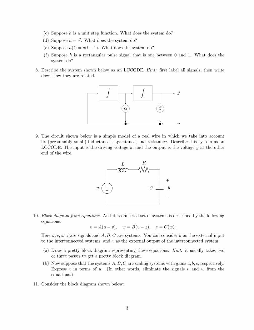
8. Describe the system shown below as an LCCODE. Hint: first label all signals, then writedown how they are related.
∫ ∫y
u
α β
9. The circuit shown below is a simple model of a real wire in which we take into accountits (presumably small) inductance, capacitance, and resistance. Describe this system as anLCCODE. The input is the driving voltage u, and the output is the voltage y at the otherend of the wire.
u y
L
C
R
10. Block diagram from equations. An interconnected set of systems is described by the followingequations:
v = A(u − v), w = B(v − z), z = C(w).
Here u, v, w, z are signals and A, B, C are systems. You can consider u as the external inputto the interconnected systems, and z as the external output of the interconnected system.
(a) Draw a pretty block diagram representing these equations. Hint: it usually takes twoor three passes to get a pretty block diagram.
(b) Now suppose that the systems A, B, C are scaling systems with gains a, b, c, respectively.Express z in terms of u. (In other words, eliminate the signals v and w from theequations.)
11. Consider the block diagram shown below:
3

u y
a
b
c
The triangle shaped blocks represent scaling systems with gains a, b, and c.
Find a simple mathematical expression for the output y in terms of the input u and theconstants a, b, and c. Your answer should be only in terms of the input u and the scalefactors a, b, and c.
12. Commuting systems. We say that two systems A and B commute if the composition orcascade connection of A and B is the same in either order, i.e., A(B(u)) = B(A(u)) for anysignal u. For example, a linear system commutes with any scaling system (that’s what itmeans for a linear system to be homogenous).
Which pairs of the following systems commute?
• a scaling system with gain 3
• an inverter, i.e., a scaling system with gain −1
• a delay system with delay 2sec
• a S/H operating at 1 sample/sec: y(t) = u(btc)• an integrator
• a 1-bit limiter
• a 1-second averaging system: y(t) =∫ tt−1 u(τ) dτ
• a square-law system, for which y(t) = u(t)2
(Every system commutes with itself. That leaves 28 other pairs of systems for you to thinkabout . . . )
You might want to organize your answer in a table. You do not have to justify your answers.
13. Find the Laplace transform of the following functions.
(a) f(t) = (1 + t − t2)e−3t.
(b) f(t) =
0 0 ≤ t < 11 1 ≤ t < 2
−1 2 ≤ t
(c) f(t) = 1 − e−t/T where T > 0.
4

14. Laplace transform monotonicity properties. Let f and g be two real-valued functions (orsignals) defined on t|t ≥ 0. Let F and G denote the Laplace transforms of f and g,respectively. We will assume that f and g are bounded, so the Laplace transforms are definedat least for all s with <s > 0.
(a) Suppose that f(t) ≥ g(t) for all t ≥ 0. Is it true that F (s) ≥ G(s) for all real, positives? If true, explain why. If false, provide a counterexample.
(b) Is the converse true? That is, if F (s) ≥ G(s) for all real positive s, is it true thatf(t) ≥ g(t) for t ≥ 0? If true, explain why. If false, provide a counterexample.
15. Laplace transform of reversed signal. So, you thought we covered all the Laplace transformrules in lecture 3? Suppose f is a signal that only lasts T seconds, i.e., f(t) = 0 for t > T .Define the signal g by ‘reversing’ f , i.e., g(t) = f(T − t) for 0 ≤ t ≤ T , and g(t) = 0 for t > T .Express G, the Laplace transform of g, in terms of F , the Laplace tranform of f .
16. Convolution and the Laplace transform.
(a) Evaluate h(t) = e−t ∗ e−2t using direct itegration. (These signals are not defined fort < 0.)
(b) Find H, the Laplace transform of h, using the expression for h you found in part (a).
(c) Verify that H is the product of the Laplace transforms of e−t and e−2t.
17. The “raised cosine pulse” is a signal used in applications such as radar and communications.It is defined by
f(t) =
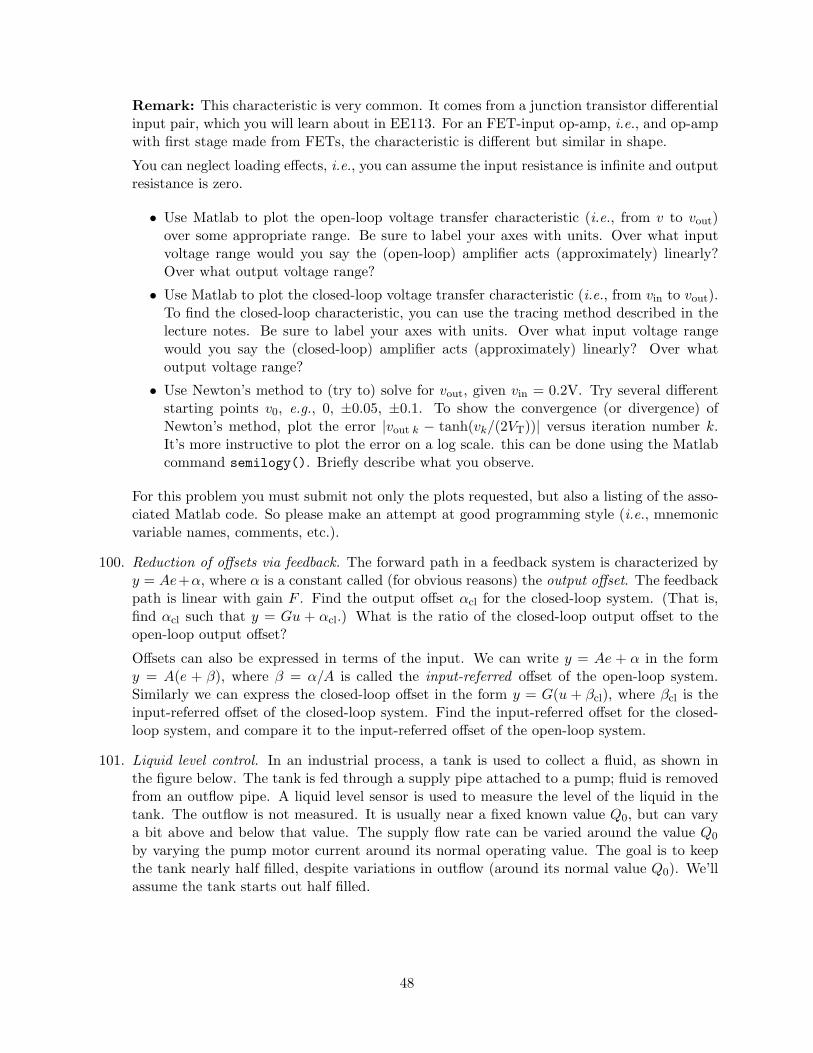
1 − cos t 0 ≤ t ≤ 2π0 t > 2π
and plotted below.
00
0.5
1
1.5
2
2.5
tπ 2π 3π 4π
f(t
)
Find F , the Laplace transform of f .
18. Consider the system shown below.
∫∫∫u y
5

(a) Express the relation between u and y as an LCCODE. Hint: if the signal z is the outputof an integrator, then its input is the signal z′.
(b) Assuming that y(0) = y′(0) = y′′(0) = 0, derive an expression for Y (the Laplacetransform of y) in terms of U (the Laplace transform of u).
19. Solve the following LCCODEs using Laplace transforms. Verify that the solution you findsatisfies the initial conditions and the differential equation.
(a) dv/dt = −2v + 3, v(0) = −1.(b) d2i/dt2 + 9i = 0, i(0) = 1, di/dt(0) = 0.
20. Four signals a, b, c, and d are related by the differential equations
a′ + a = b, b′ + b = c, c′ + c = d,
where a(0) = b(0) = c(0) = 0. Express A(s), the Laplace transform of a, in terms of D(s),the Laplace transform of d.
21. The Laplace transform of a signal q is given by
Q(s) =3 − 5e−s
s + 1.
Find q (i.e., describe it explicitly).
22. A signal z satisfies z′′′ + z′′ + z′ + z = 0, and z(0) = z′(0) = 0, z′′(0) = 1. Find z.
23. In the system shown below, k is a gain.
∫∫k
y
(a) For what values of k is this system stable?(b) For what values of k is this system stable and critically damped?(c) For what values of k do (nonzero) solutions y change sign infinitely often? (We do not
require stability here.)
24. Unity feedback around amplifier. The system shown below consists of an amplifier of gain a,connected in what is sometimes called a unity feedback configuration. (We’ll study feedbackin more detail later in the course.)
u ya
6

(a) Solve for y(t) in terms of u(t). Your answer should come out in the form y(t) = bu(t)for some scalar b, which is called the closed-loop gain of the feedback configuration. Youcan assume that a 6= 1.
(b) What is the closed-loop gain b, when a = 0.9? When a is positive and near but smallerthan one, the system is sometimes described as regenerative. (Can you explain why thisname is used?) This configuration is sometimes used to get more gain from a device oramplifier than you would otherwise have.
(c) The feedback configuration is often used when a is large and negative, say, a ≈ −104.In this case the system is referred to as a following amplifier. (Can you guess why?)What is b is this case? How much does b vary as a varies over the 100-fold range froma = −103 to a = −105? The answer shows one of the reasons this configuration is used.
25. Convolution and Laplace transforms. Let u denote a unit rectangular pulse signal that startsat t = 0 and lasts until t = 1.
(a) Find the signal v = u ∗ u by evaluating the convolution integral directly. Sketch u andv = u ∗ u. Hint: v is sometimes called a triangular pulse signal.
(b) Find U and V , the Laplace transforms of u and v, respectively, by directly evaluating theLaplace transform defining integrals using the expressions for u and v found in part a.Hint: the indefinite integral of te−st is − (
t/s + 1/s2)e−st.
(c) Find V from U using the convolution formula for Laplace transforms and verify you getthe same result.
26. Thermal runaway. A conductor with resistance R carries a fixed positive current i, and hencedissipates a power P = i2R. This causes the conductor to heat up (hopefully not too much)above the ambient temperature.
Let T (t) denote the temperature of the conductor above the ambient temperature at time t.T satisfies the equation
aT ′ = −bT + P
where a > 0 is the thermal capacity of the conductor (in J/C), b > 0 is the thermalconductivity (in W/C), and P is the power (in W) dissipated in the conductor.
The resistance R of the conductor changes with temperature according to
R = R0(1 + cT )
where the constant c (which has units 1/C) is called the resistance temperature coefficient(or just ‘tempco’) of the conductor, and R0 > 0 is the resistance of the conductor at ambienttemperature. Depending on the material of the conductor, the tempco c can be positive ornegative; for example, for metal wires the tempco is positive. (The formula above is validonly over a range where 1 + cT > 0.)
(a) Consider a metal wire, for which c > 0. If the current i is smaller than a critical valueicrit, the temperature T converges to a steady-state value as t → ∞. If the current iis larger than this critical value of current, then the temperature T converges to ∞ ast → ∞. (In practice, the temperature increases until the conductor is destroyed, e.g.,melted.) This phenomenon is called thermal runaway.Find the critical value icrit, above which thermal runaway occurs. Express the answerin terms of the other constants in the problem (a, b, R0, c).
7

(b) Suppose the wire is initially at ambient temperature, i.e., T (0) = 0, and the constantshave the values
a = 1J/C, b = 0.5W/C, i = 10A, R0 = 1Ω, c = 0.01/C
Find T (t) for t ≥ 0
27. A voltage v(t) is applied to a DC motor. A simple electrical model of the motor is aninductance L in series with a resistance R, so the motor current i(t) satisfies
Ldi/dt + Ri = v.
The motor shaft angle is denoted θ(t), and the shaft angular velocity ω(t) (so we have ω =dθ/dt). The motor current puts a torque on the shaft equal to ki(t), where k is the motorconstant. The shaft rotational inertia is J and the damping coefficient is b. Newton’s equationis then:
Jdω/dt = ki − bω.
Assuming that i(0) = 0, θ(0) = 0, and ω(0) = 0, express Θ (the Laplace transform of θ) interms of V (the Laplace transform of v).
The numbers L, R, k, J, b are all positive constants.
28. What does the following circuit do? Assume v1(0) = 0 and v2(0) = 1.
Hint: Show that d2v1(t)/dt2 + ω2v1(t) = 0, where ω = 1/(10kΩ · 0.01µF).
v1(t) v2(t)
.01µF .01µF10kΩ
10kΩ
10kΩ10kΩ
29. An RCRC circuit. Consider the circuit shown below. For t < 0, vin(t) = 1V and the circuitwas in static conditions. For t ≥ 0, vin(t) = 0V.
vin(t) vout(t)
1Ω 1Ω
1F 0.5F
8

(a) Find vout at t = 0, immediately after vin has switched to 0V.
(b) Finddvout
dtat t = 0, immediately after vin has switched to 0V.
(c) Find vout at t = 1.
30. The waveform shown below is the current in a series RLC circuit. The value of the resistoris 100Ω.
-1
-0.8
-0.6
-0.4
-0.2
0
0.2
0.4
0.6
0.8
1
0 2 4 6 8 10 12 14 16
t (sec)
i(t)
(A)
(a) Estimate L and C.
(b) About how long will it be before 99% of the initial stored energy in the circuit hasdissipated?
31. Adding inductance to improve decay rate of a cable. A long cable, driven by a voltage sourceat one end and with a high impedance load at the other, is modeled as a resistance Rcable,inductance Lcable, and capacitance Ccable, as shown below.
vin vout
Rcable
Ccable
Lcable
9

As a measure of how fast the cable can react to the driving voltage, we use the decay rate ofthe system, when the voltage source vin switches to 0V and stays at 0V. Recall that the decayrate is defined as D = −max<λ1,<λ2, where λ1 and λ2 are the roots of the characteristicpolynomial of the system (with vin = 0). Thus, the system has positive decay rate, and alarger decay rate means that vout converges to zero faster.
An engineer suggests that adding an extra inductance Lextra in series with the driving voltage,as shown below, might increase the decay rate of the cable.
vin vout
Rcable
Ccable
LcableLextra
A second engineer responds: “Adding inductance is crazy! It’s precisely the inductance thatslows the cable, by fighting changes in current. Adding inductance will make the cable systemslower, i.e., decrease the decay rate.”
For the rest of this problem you can use the specific values
Rcable = 2000Ω, Lcable = 100µH, Ccable = 0.01µF.
Finally, the problem: find the value of Lextra that yields the maximum possible decay ratefor the cable. (Of course you must have Lextra ≥ 0.)
If your choice is Lextra = 0, you are agreeing with the second engineer quoted above.
Explain the reasoning behind your choice of Lextra. We want a specific number for Lextra, nota formula involving other problem parameters.
32. The RLRC circuit. In the series RLC circuit, current flow causes power to be dissipated inthe resistor as heat. In the parallel RLC circuit, voltage causes power to be dissipated. Inthe RLRC circuit shown below, power is dissipated by both mechanisms.
Rp
Rs
CvC
iL
L
(a) Find an LCCODE of the form
av′′c + bv′c + cvc = 0
that describes this circuit.
10

(b) Find an expression for the rate of change of the total stored energy, i.e.,
d
dt
(LiL(t)2
2+
CvC(t)2
2
),
in terms of iL(t) and vC(t). Give one sentence interpreting your result.
33. Transition from overdamped to critically damped to underdamped. Consider three series RLCcircuits with the same inductance and capacitance, L = 1H, C = 1F, and the same initialconditions: 1V across the capacitor and zero current in the circuit. The resistors in the threecircuits differ slightly: in the first circuit we have R = 1.99Ω; in the second circuit we haveR = 2Ω, and in the third circuit we have R = 2.01Ω.
1H 1F
R
v(t)
You know from lecture 4 that the formulas for the solution v(t) (the voltage across thecapacitor) of these three circuits are quite different: In the first case, v(t) is an exponentiallydecaying sinusoid; in the second, it is the sum of an exponential and a term involving t timesan exponential; in the last case, v(t) is a sum of two decaying exponentials.
One student says:
The voltage response is quite different in these three cases: in the first case thevoltage crosses the value zero infinitely often; in the second and third cases, just onceor maybe twice. So the solutions of these three circuits are indeed very different,even though the three resistor values are so close. The reason is that the valueR = 2Ω is a “critical value” for this circuit, as seen in the formulas for lecture 4.It’s not surprising that the solution of a circuit changes drastically as the resistancevaries near a “critical value”.
A second student then responds:
Something is fishy here. I don’t see how such a miniscule change in the resistorvalue can have such a great effect on the voltage across the capacitor. It justdoesn’t make physical sense to me. In fact, now that I think about it, exact criticaldamping can never be achieved in practice since it requires knowing the inductance,capacitance, and resistance with infinite precision, which is impossible.
(a) Who is right? Briefly discuss.
(b) Check your claims by plotting the three voltage waveforms using Matlab. (You mightneed to go back and change your answer to (a)!)
34. In the circuit shown below, vout(0) = 0 and vin(t) = 1 − e−2t for t ≥ 0.
11

vin(t) vout(t)1F
1Ω
Find the output voltage, vout(t), for t ≥ 0.
35. The vertical dynamics of a vehicle suspension system, when the vehicle is driving on levelground, are given by
(mv + ml)d′′(t) + bd′(t) + kd(t) = 0.
Here
• t is time (in seconds)
• d(t) is the vertical displacement of the vehicle, with respect to its neutral position (inmeters)
• mv = 103kg is the vehicle mass
• ml ≥ 0 (also given in kg) is the mass of the vehicle load (passengers, cargo, etc.)
• b = 2.2 · 104N/m/s is the suspension damping
• k = 105N/m is the suspension stiffness
The initial conditions are d(0) = 0.1m, d′(0) = 0m/s.
What is the smallest load mass ml for which d is oscillatory? (By oscillatory, we mean thatd(t) passes through zero infinitely many times.)
36. Stopping a DC motor.
motor
shaft
v
i
A DC motor is characterized by v = kω + Ri + Li′ where
• v is the voltage at its electrical terminals
• i is the current flowing into its electrical terminals
• ω is the rotational velocity of its shaft (in rad/sec)
• R is the resistance of the motor winding
• L is the inductance of the motor winding
12

• k is a constant called the motor constant
The resulting torque on the shaft is given by τ = ki.
A common mechanical model for the shaft and its load is a mechanical resistance b and arotational inertia J . Newton’s law, which states that Jω′ is equal to the total applied torqueon the shaft, is then Jω′ = −bω + τ .
To simplify your calculations, we’ll assume the constants are
R = 1, L = 1, k = 1, J = 1, b = 1
(with, of course, the appropriate physical units).
For t < 0, the motor is used for some purpose (which doesn’t concern us), so we have some(nonzero) initial current i(0) and initial rotational velocity ω(0).
Our job is to stop the motor for t ≥ 0, i.e., cause ω(t) to converge to zero as t → ∞. Thisis done by connecting its terminals to a resistance Rext ≥ 0 (the subscript ‘ext’ stands for‘external’), which results in v = −Rexti.
What value of Rext results in the motor velocity ω converging to zero fastest?
One engineer argues that the best thing to do is to set Rext = 0, i.e., just short circuit themotor. His argument is very simple: “applying a voltage to the motor is what makes it go,so to make it stop, set the voltage to zero by shorting the motor.”
Do you agree? (I.e., is the best value Rext = 0?)
37. For each of the following rational functions, find the poles and zeros (giving multiplicities ofeach), the real factored form, the partial fraction expansion, and inverse Laplace transform.(In some cases, the expression may already be in one of these forms.)
(a)1
s + 1+
1s + 2
+1
s + 3
(b)s2 + 1s3 − s
(c)(s − 2)(s − 3)(s − 4)
s4 − 1
38. Response of an RC circuit to a voltage ramp. In the simple RC circuit shown below, thesource voltage is given by
vin(t) =
0 t < 0t t ≥ 0
(which is called a 1V/sec voltage ramp). The capacitor is uncharged at t = 0.
Find vout(t) for t ≥ 0.
vin(t) vout(t)1F
1Ω
13

39. In the circuit below, vin(t) = 1− e−2t for t ≥ 0, and the capacitor is uncharged at t = 0. Findvout(t) for t ≥ 0.
vin vout1Ω
1F
40. In the circuit below, the current i is a unit ramp at t = 0, i.e., i(t) = t for t ≥ 0. The inductorcurrent and capacitor voltage are both zero at t = 0.
Find v(t) for t ≥ 0.
i 0.5F 2H v
41. Four functions f1, f2, f3, and f4, are shown below. Their Laplace transforms are F1, F2, F3,and F4, respectively. You can assume F1, . . . , F4 are rational functions, with no more thanthree poles (counting multiplicities).
Please note carefully the vertical scales — they are not the same!
14

0 2 4 6−3
−2
−1
0
1
2
0 2 4 6−4
−3
−2
−1
0
1
2
0 2 4 6−4
−3
−2
−1
0
1
2
0 2 4 6−15
−10
−5
0
f 1(t
)
f 2(t
)
f 3(t
)
f 4(t
)
tt
tt
Estimate the poles of F1, . . . , F4, using the smallest number needed to give a reasonablematch. If you can get a reasonable match with one pole, then give just one pole; if two polessuffice then give just two. Give three poles only if three poles are required to match the givenfi.
• We want specific numbers, not just qualitative answers such as ‘one positive real, onecomplex pair’ or σ + jω (without specifying σ or ω). Make clear indications on the plotshow you got the numbers.
• Give complex poles separately, as in ‘1 + j, 1 − j’; we will not automatically supplyconjugates of complex numbers.
• Give multiple poles by repeating them in your answers, e.g., ‘−3, −1, −1’ (meaning, onepole at s = −3, and another pole of multiplicity two at s = −1).
42. In the circuit below, the capacitors are uncharged at t = 0, the voltages vin and vout arereferenced to ground, and the op-amp is ideal.
vin(t)vout(t)
1Ω
2Ω
1F
1F
15

Find the DC gain, poles, and zeros of the transfer function from vin to vout. If the polesand/or zeros ar repeated, be sure to give the multiplicity.
43. In the circuit below, the capacitors are uncharged at t = 0, the voltages vin and vout arereferenced to ground, and the op-amp is ideal.
vin(t)vout(t)
R1
R2
C1
C2
(a) Find the poles and zeros of the transfer function from vin to vout. If the poles and/orzeros are repeated, be sure to give the multiplicity.
(b) Now let R2 = 1Ω. Find numerical values for R1, C1, and C2, so that the impulse responsefrom vin to vout is 2e−2t − 3e−3t. (There might be several solutions; we just want one.)
44. Pharmacokinetics. When a drug is administered to a patient, its concentration first rapidlyincreases, and then decays over a much longer period. The period of rapid increase is calledthe uptake phase, and the period of slower decay is called the absorption or decay phase.
The figures below shows a typical plot of concentration x(t) versus time, with t measured inhours after the drug is administered. (The concentration might be measured in milligrams/cm3,but it doesn’t matter to us.) The first plot shows the concentration x(t) over a time range0 ≤ t ≤ 20, which shows the decay phase well. The second plot shows the same concentrationx(t) over the shorter range 0 ≤ t ≤ 1, which shows the uptake phase well.
16

0 2 4 6 8 10 12 14 16 18 200
0.2
0.4
0.6
0.8
0 1 20
0.2
0.4
0.6
0.8
t
t
x(t
)x(t
)
A common (approximate) model is that the concentration x satisfies a second order au-tonomous LCCODE:
x′′ + bx′ + cx = 0.
Estimate the coefficients b and c that (approximately) describe the x(t) shown in the twoplots above.
You must explain how arrive at your estimates.
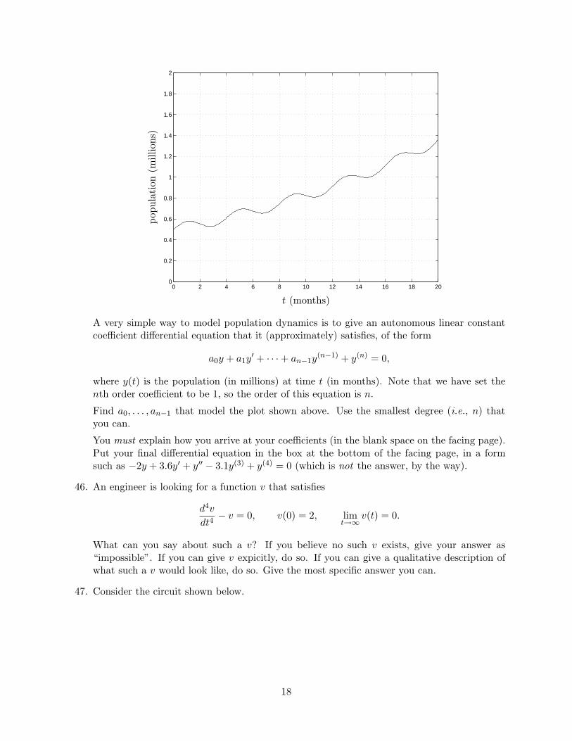
45. Modeling population dynamics. The plot below shows the population (in millions) of somespecies over a period of 20 months. (The population is so large that we consider it to be areal number, ignoring the fact that it must be an integer.) As you can see, it is characterizedby periodic oscillations above and below a steady growth.
17
0 2 4 6 8 10 12 14 16 18 200
0.2
0.4
0.6
0.8
1
1.2
1.4
1.6
1.8
2
t (months)
popu
lati
on(m
illio
ns)
A very simple way to model population dynamics is to give an autonomous linear constantcoefficient differential equation that it (approximately) satisfies, of the form
a0y + a1y′ + · · · + an−1y
(n−1) + y(n) = 0,
where y(t) is the population (in millions) at time t (in months). Note that we have set thenth order coefficient to be 1, so the order of this equation is n.
Find a0, . . . , an−1 that model the plot shown above. Use the smallest degree (i.e., n) thatyou can.
You must explain how you arrive at your coefficients (in the blank space on the facing page).Put your final differential equation in the box at the bottom of the facing page, in a formsuch as −2y + 3.6y′ + y′′ − 3.1y(3) + y(4) = 0 (which is not the answer, by the way).
46. An engineer is looking for a function v that satisfies
d4v
dt4− v = 0, v(0) = 2, lim
t→∞ v(t) = 0.
What can you say about such a v? If you believe no such v exists, give your answer as“impossible”. If you can give v expicitly, do so. If you can give a qualitative description ofwhat such a v would look like, do so. Give the most specific answer you can.
47. Consider the circuit shown below.
18

2 + 4 cos t
1H
1Ω1F vout
(a) Suppose that the circuit is in periodic steady-state. Find vout(t).
(b) Suppose that the inductor current and capacitor voltage at t = 0 are both zero. Findvout(t). Does vout(t) converge to the periodic steady-state solution you found in part(a), as t → ∞? What are the poles of the Laplace transform of vout?
48. How critical is critical damping? We consider the second order LCCODE ay′′ + by′ + cy = 0,with a, b, c > 0. We assume that a and c are fixed, and consider the effect of the parameter bon the asymptotic decay rate of the system, defined as D = −max<λ1,<λ2, where λi areroots of the characteristic polynomial. (Thus, D is positive; large D corresponds to a fastdecay rate.) You know that the choice of b given by b = bcrit = 2
√ac gives the maximum
value of D, which is Dcrit =√
c/a.
Find the range of b for which the decay rate is at least 90% of the maximum possible decayrate, Dcrit. If you can express your answer as a percentage above and below bcrit, do so.
49. Suppose that f satisfies d3f/dt3 = f , f(0) = 1, df/dt(0) = d2f/dt2(0) = 0. Find f(t).
50. Positive real zeros and sign changes in f . Suppose that F (z) = 0 for some real, positive z.You may assume that z is such that the defining integral for the Laplace transform converges.Show that f must change sign, i.e., assume both negative and positive values at various times.Another way to say this is, f cannot be nonnegative for all t ≥ 0 or nonpositive for all t ≥ 0.
51. Defibrillators. (This problem is from EE101, and is here because the next problem continuesit.) A defibrillator is used to deliver a strong shock across the chest of a person in cardiacarrest or fibrillation. The shock contracts all the heart muscle, whereupon the normal beatingcan (hopefully) start again. The first defibrillators used the simple circuit shown below.
vs
Rth = 10kΩ
Rchest = 500ΩC = 20µF
S D
With the switch in the standby mode, indicated as ‘S’, the 20µF capacitor is charged up bya power supply represented by a Thevenin voltage vs and Thevenin resistance Rth = 10kΩ.When the switch is thrown to ‘D’ (for ‘defibrillate’), the capacitor discharges across the
19

patient’s chest, which we represent (pretty roughly) as a resistance of 500Ω. (The connectionsare made by two ‘paddles’ pushed against the sides of the chest.)
On most defibrillators you can select the ‘dose,’ i.e., total energy of the shock, which is usuallybetween 100J and 400J.
(a) Find vs so that the dose is 100J. You can assume the capacitor is fully charged whenthe switch is thrown to ‘D’. We’ll use this value of vs in parts 1b, 1c, and 1d.
(b) How long after the switch is thrown to ‘D’ does it take for the defibrillator to deliver90% of its total dose, i.e., 90J?
(c) What is the maximum power pmax dissipated in the patient’s chest during defibrillation?
(d) Our model of the chest as a resistance of 500Ω is pretty crude. In fact the resistancevaries considerably, depending on, e.g., skin thickness. Suppose that the chest resistanceis 1000Ω instead of 500Ω. What is the total energy E dissipated in the patient duringdefibrillation?
52. An improved defibrillator. One problem with the defibrillator described in problem 1 is thatthe maximum power pmax (which you found in part 1c) is large enough to sometimes causetissue damage. An electrical engineer suggested the modified defibrillator circuit shown below.The inductor is meant to ‘smooth out’ the current through the chest during defibrillation,and yield a lower value of pmax for a given dose.
vs
Rth = 10kΩ
Rchest = 500Ω
L
C = 20µF
S D
(a) Find the value of L that yields critical damping. We’ll use this value of L in parts 2band 2c.
(b) Find vs so that the dose is 100J. You can assume the capacitor is fully charged whenthe switch is thrown to ‘D’.
(c) Suppose vs is equal to the value found in part 2b. What is the maximum power pmax
dissipated in the patient’s chest during defibrillation?
53. Consider the circuit shown below. You can assume the capacitor voltage and the inductorcurrent are zero at t = 0.
20

1H0.25F
1Ωvin(t)
vout(t)
Two plots are shown below. The top plot shows the unit step response from vin to vout,i.e., vout(t) with vin(t) = 1. Note that it exhibits some ringing, i.e., oscillation, and settles(converges) in about 5sec or so.
The bottom plot shows the desired output voltage, which is vdes(t) = 1 − e−3t. Note that itexhibits no oscillation and settles quite a bit faster than the step response, i.e., in about 1sec.
0 1 2 3 4 5 6 7 8 9 100
0.5
1
1.5
2
0 1 2 3 4 5 6 7 8 9 100
0.5
1
1.5
2
t
t
v out(
t)v d
es(t
)
Unit step response
Desired output response
Finally, the problem: can you find an appropriate vin(t) such that we have vout = vdes?
If there is no such vin, give your answer as “impossible”. Otherwise, give vin that yieldsvout = vdes.
54. In the circuit shown below, vout(0) = 0 and vin(t) = 1 − e−2t for t ≥ 0. Find the Laplacetransform Vin(s) of vin(t). Find the output voltage, vout(t), for t ≥ 0. (Not just its Laplacetransform.)
21

vin(t) vout(t)1F
1Ω
55. Reducing the rise-time of a signal. In a certain digital system a voltage signal should ideallyswitch from 0V to 5V infinitely fast, i.e., with zero rise-time. But due to the finite bandwidthof the electronics that generates the signal, it has the form
vin(t) = 5(1 − e−t/T
)for t ≥ 0
where T = 1µsec. Thus, the signal has a rise-time around a few µsec.
An engineer claims that the circuit shown below can be used to reduce the rise-time of thesignal, provided the component values R and C are chosen correctly. Specifically, the engineerclaims that by choosing R and C correctly, we can have
vout(t) = a(1 − e−10t/T
)for t ≥ 0
where a is some nonzero constant. Thus, the rise-time of vout is a factor of 10 smaller thanthe rise-time of vin, i.e., a few hundred nsec.
vin(t) vout(t)R
C
1kΩ
Here is the problem: determine whether the engineer’s claim is true or false. If the claim istrue, find specific, numerical values of R and C that validate the claim. If the claim is false,briefly explain why the engineer’s idea will not work.
(You can assume the circuit starts in the relaxed state, i.e., no charge on the capacitor. Andno, you cannot use negative R or C.)
56. The top plot below shows the step response of a system described by a transfer function.Below that is a plot of an input u(t) that we apply to this system. Sketch the response(output) y(t).
22

0 0.5 1 1.5 2 2.5 3 3.5 4 4.5 5-0.5
0
0.5
1
1.5
0 0.5 1 1.5 2 2.5 3 3.5 4 4.5 5-0.5
0
0.5
1
1.5
s(t)
u(t
)
t (nsec)
t (nsec)
57. Find the unit step response, from input current to shaft angle, of the DC motor describedin lecture 8. What is the asymptotic angular velocity, i.e., what does the angular velocityapproach as t increases? Can you give a physical interpretation of your result?
58. In the circuit shown below you may assume the op-amp is ideal, and the voltage across eachof the capacitors is zero at t = 0.
vin(t)
2Ω
1Ω
1F
1F
vout(t)
(a) Find the transfer function H from vin to vout. Try to express H in simple form.
(b) Find the poles, zeros and DC gain of H.
(c) Suppose that vin(t) = 1 for t ≥ 0. Find vout(t).
23

59. In the circuit below, vin(t) = 2 sin(5t) for t ≥ 0, R1 = R2 = 1Ω, C = 1F , and the capacitoris initially uncharged at t = 0. Find vout(t) for t ≥ 0.
vin
R1
R2 C vout
60. A cascade system with repeaters. This problem concerns the block diagram shown below.The system consists of four cascaded subsystems: two identical channels, denoted C, and twoidentical repeaters, denoted R. The input signal u first propagates through a channel, thena repeater, then another channel, and finally a repeater.
C R C Ru v w y z
Each channel C is described by a differential equation relating its input and output. If a isthe input signal and b is the output signal of C, i.e., b = Ca, we have
b′ + b = a.
You can assume that the initial condition of each of the channels is zero, i.e., v(0) = y(0) = 0.
The repeaters are described as follows. If a is the input signal to a repeater R and b is theoutput signal (i.e., b = Ra), we have
b(t) =
1 if a(t) ≥ 0.50 if a(t) < 0.5
for all t ≥ 0. In other words, the repeater puts out 1 when the input signal is at least thethreshold value 0.5, and puts out 0 when the input signal is less than the threshold.
Finally, the problem. The input signal u is a unit step at t = 0, i.e., u(t) = 1 for t ≥ 0. Findthe output signal z.
61. Pole location mix and match. The plots shown at the end of this problem show five differentsignals (i.e., functions of time), labeled a, b, c, d, and e.
We are interested in the poles of the Laplace transform of each signal. For each signal, identifythe poles from the eight choices given below, which are labeled I, . . . , VIII. For example,give your answer for b as II, if you believe that B(s) has two poles, at s = −2 + 0.3j ands = −2 − 0.3j.
Here are the choices for poles (which include multiplicities):
24

I: −0.2 + j, −0.2 − j
II: −2 + 0.3j, −2 − 0.3j
III: −4, −0.01
IV: 0, −0.2 + j, −0.2 − j
V: 0.4, −12
VI: −0.05 + j, −0.05 − j, 0.015 + j, 0.015 − j
VII: −0.05, 0.015 + j, 0.015 − j
VIII: 0, 0, −1
Each of these choices of poles corresponds to at most one of the given signals, though, ofcourse, some of the above choices correspond to none of the signals. Please note that thescales of the plots matter!
25

0 1 2 30
0.5
1
1.5
2
2.5
3
3.5
0 1 2 3 40
0.1
0.2
0.3
0.4
0.5
0 10 20 30 40−0.5
0
0.5
1
1.5
0 5 10 150.2
0.4
0.6
0.8
1
1.2
0 100 200 300−1.5
−1
−0.5
0
0.5
1
1.5
a(t
)
b(t)
c(t)
d(t
)
e(t)
t
tt
tt
62. Oscillation frequencies of a coupled mass-spring system.
This problem concerns the mechanical system shown below. A mass m1 is connected via aspring with stiffness k1 to a rigid wall (shown as the dark bar at left) and also, via a springwith stiffness k2, to a second mass m2. The displacements of the masses (with respect to theequilibrium positions) are denoted d1(t) and d2(t), respectively.
26

k1 k2
d1(t) d2(t)
m1 m2
This two mass system is governed by Newton’s equations of motion, which are
m1d′′1 = −k1d1 + k2(d2 − d1), m2d
′′2 = −k2(d2 − d1).
For simplicity, we’ll use the specific numbers
m1 = m2 = 1kg, k1 = k2 = 1N/m,
(and, of course, we measure t in seconds and the displacements in meters).
The general form of d2 (and, for that matter, d1) is given by
d2(t) = A1 cos(ω1t + φ1) + A2 cos(ω2t + φ2),
where the constants A1, A2, φ1, φ2 are determined by the initial conditions. Find the twofrequencies ω1 and ω2. You can give your answer in an analytical form, or in numerical form(to three significant figures).
63. The system shown below is described by a transfer function G. The poles of G are at s = −1and s = −4; G has only one zero, at s = −2. The DC gain of G is 1.
u(t) y(t)G(s)
(a) Find the impulse response g(t) of this system.
(b) Suppose that u(t) = e−2t for t ≥ 0. Find y(t).
64. The signals f and g are plotted below. Plot f ∗ g.
27

0 0.5 1 1.5 2 2.5 3 3.5 4 4.5 5-1.5
-1
-0.5
0
0.5
1
0 0.5 1 1.5 2 2.5 3 3.5 4 4.5 5-1.5
-1
-0.5
0
0.5
1
t
t
f(t
)g(t
)
65. The circuit below is a simple one-pole lowpass filter.
vin(t)
vout(t)
10kΩ
R
C
Find (positive) R and C such that:
• The (magnitude of the) DC gain is +12dB.
• The magnitude of the transfer function at the frequency 1kHz is 3dB less than themagnitude of the DC gain.
You can assume the op-amp is ideal. Give numerical values for R and C. An acurracy of 10%will suffice.
66. A feedback system with two disturbances. The system below shows a feedback system, withinput u, output y, and two disturbance signals, d1 and d2 (that are also input signals). The
28
two systems A and B are scalar gains, with gains α and β, respectively. (In this context αis called the forward gain and β is called the feedback gain.) Note that on the left we have adifference junction; on the right and bottom we have summing junctions.
A
B
u y
d1
d2
(a) Express y in terms of u, d1, and d2. You can assume that αβ 6= −1.
(b) Now consider the (typical) values α = 105, β = 10−2. Which of the two disturbances hasa greater effect on the output y, assuming the disturbances have the same size? Youranswer must be one of:
• d1 (i.e., d1 has a greater effect on y than d2)• d2 (i.e., d2 has a greater effect on y than d1)• the same (i.e., d1 and d2 have the same effect on y)• can’t determine (i.e., we can’t determine which disturbance has the greater effect
on y, from the data given)
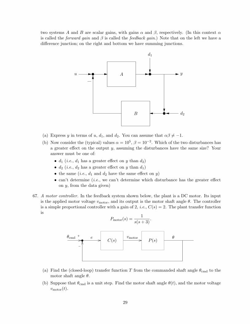
67. A motor controller. In the feedback system shown below, the plant is a DC motor. Its inputis the applied motor voltage vmotor, and its output is the motor shaft angle θ. The controlleris a simple proportional controller with a gain of 2, i.e., C(s) = 2. The plant transfer functionis
Pmotor(s) =1
s(s + 3).
vmotorθcmd θeP (s)C(s)
(a) Find the (closed-loop) transfer function T from the commanded shaft angle θcmd to themotor shaft angle θ.
(b) Suppose that θcmd is a unit step. Find the motor shaft angle θ(t), and the motor voltagevmotor(t).
29

68. A simple two-way crossover circuit. A typical high-fidelity speaker has separate drivers forlow and high frequencies. (The driver is the physical device that vibrates to create the soundyou hear. The old terms for the low and high frequency drivers are woofer and tweeter,respectively.)
The circuit shown below, called a speaker crossover network, is used to divide the audio signalcoming from the amplifier into a low frequency part for the low frequency driver (LFD) and ahigh frequency part for the high frequency driver (HFD). Since the audio spectrum is dividedinto two parts, this is called a two-way system (three-way are also common).
The amplifier is modeled as a voltage source (which is a very good model), and the low andhigh frequency drivers are modeled as 8Ω resistances (which is not a good model of realdrivers, but we will use it for this problem).
vamp(t)
8Ω 8Ω
C L
speaker
HFD LFD
Zspeaker
The crossover network is designed so that the transfer function from the amplifier to eachdriver has magnitude −3dB at a frequency ωc called the crossover frequency of the speaker.
(a) Choose C and L so that the crossover frequency is 2kHz. Do this carefully as you willneed your answers in part b.
(b) Using the values for L and C found in 8a and 8b, find Zspeaker(s), the impedance of thetwo-way speaker seen by the amplifier (as indicated in the schematic).
69. Stability analysis of a PI controller. Suppose that PI control,
C(s) = kp +ki
s,
is used with the plant
P (s) =1
s2 + 2s + 2,
in the standard feedback control configuration:
r yPC
30

Find the conditions on kp and ki for which the closed-loop transfer function T from r to y isstable. You can assume that kp > 0 and ki > 0.
Express your conditions in the simplest form possible.
70. Local versus global feedback: dynamic analysis. We consider two amplifiers, each with atransfer function H(s) = 100/(1 + s). We are going to use these amplifiers, together withfeedback, to design a system with DC gain 40dB. (Roughly speaking, then, we have 40dB of‘extra’ gain.)
Global feedback. In this arrangement we connect the two amplifiers in cascade, and then usefeedback around the cascade connection, as shown below.
u yglobH(s)H(s)
fglob
Local feedback. In this arrangement we use feedback around each amplifier, and then put thetwo closed-loop systems in cascade, as shown below. (To simplify things, we’ll assume thetwo feedack gains are the same.)
u ylocH(s)H(s)
flocfloc
In both arrangements, the feedback consists of a positive gain (independent of s).
(a) Find the value of fglob that makes the closed-loop DC gain from u to yglob, in the globalfeedback arrangement, equal to 40dB.
(b) Find the value of floc that makes the closed-loop DC gain from u to yloc, in the localfeedback arrangement, equal to 40dB.We’ll define the settling time of a system as the time it takes for the unit step responseto settle to within about 10% of its final (asymptotic) value. If the system is unstable,we’ll say the settling time is ∞.
(c) Using the value for fglob found in part 3a, find the settling time Tglob of the globalfeedback system.
(d) Using the value for floc found in part 3b, find the settling time Tloc of the local feedbacksystem.
31

(e) Give a one sentence intuitive explanation of the results of 3c and 3d.
(f) You can estimate the settling times, provided you explain how you obtain the estimate.An accuracy of ±30% is fine.
71. Step response of cascaded systems. A system described by a transfer function has the stepresponse shown below.
s(t)
t
2
1
t = 1 t = 8
Now suppose that two such systems (i.e., each with the step response shown above) areconnected in cascade. At the bottom of this page sketch the step response of the resultingcascade connection. Make sure that all critical parts of your plot are clearly labeled. Be sureto make clear which portions of your plot are curved or straight.
72. The unit step response s(t) of a system described by a transfer function H, which has threepoles, is shown in the two plots below. The two plots have different ranges; the second plotallows you to see details for small t.
0 0.1 0.2 0.3 0.4 0.5 0.6 0.7 0.8 0.9 10
0.5
1
1.5
0 0.005 0.01 0.015 0.02 0.025 0.03 0.035 0.04 0.045 0.050
0.05
0.1
0.15
0.2
t
t
s(t)
s(t)
(a) Estimate the poles. An accuracy of ±20% is acceptable.
32
(b) At high frequencies |H(jω)| becomes small. From the data given, can you determinethe rate at which it decreases for large frequency (e.g., 12 db/octave)? Either give therate (in dB/octave) or state “cannot determine” if the data given is not sufficient todetermine the high-frequency rolloff rate.
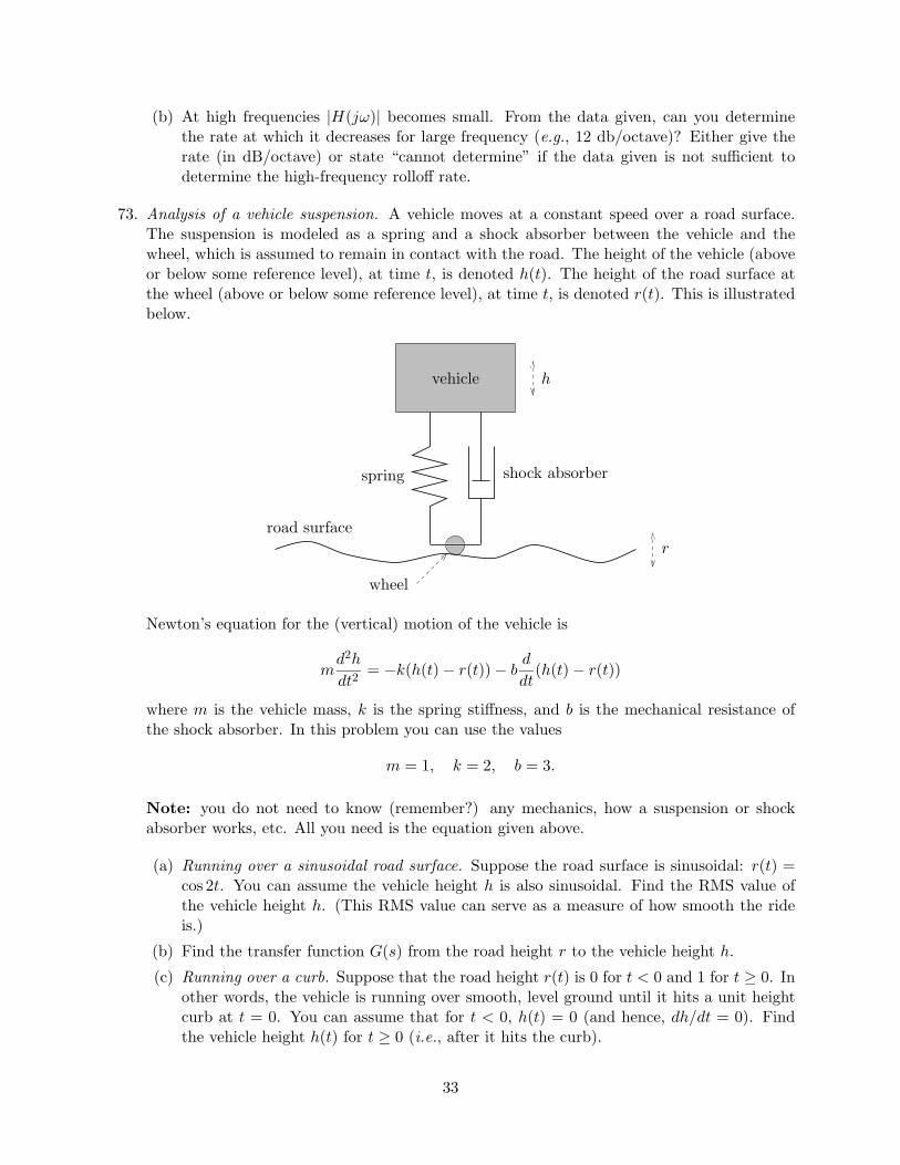
73. Analysis of a vehicle suspension. A vehicle moves at a constant speed over a road surface.The suspension is modeled as a spring and a shock absorber between the vehicle and thewheel, which is assumed to remain in contact with the road. The height of the vehicle (aboveor below some reference level), at time t, is denoted h(t). The height of the road surface atthe wheel (above or below some reference level), at time t, is denoted r(t). This is illustratedbelow.
road surface
spring shock absorber
wheel
vehicle h
r
Newton’s equation for the (vertical) motion of the vehicle is
md2h
dt2= −k(h(t) − r(t)) − b
d
dt(h(t) − r(t))
where m is the vehicle mass, k is the spring stiffness, and b is the mechanical resistance ofthe shock absorber. In this problem you can use the values
m = 1, k = 2, b = 3.
Note: you do not need to know (remember?) any mechanics, how a suspension or shockabsorber works, etc. All you need is the equation given above.
(a) Running over a sinusoidal road surface. Suppose the road surface is sinusoidal: r(t) =cos 2t. You can assume the vehicle height h is also sinusoidal. Find the RMS value ofthe vehicle height h. (This RMS value can serve as a measure of how smooth the rideis.)
(b) Find the transfer function G(s) from the road height r to the vehicle height h.
(c) Running over a curb. Suppose that the road height r(t) is 0 for t < 0 and 1 for t ≥ 0. Inother words, the vehicle is running over smooth, level ground until it hits a unit heightcurb at t = 0. You can assume that for t < 0, h(t) = 0 (and hence, dh/dt = 0). Findthe vehicle height h(t) for t ≥ 0 (i.e., after it hits the curb).
33

74. Transfer function from rainfall to river height. The height of a certain river depends on thepast rainfall in the region. Specifically, let u(t) denote the rainfall rate, in inches-per-hour, ina region at time t, and let y(t) denote the river height, in feet, above a reference (dry period)level, at time t. The time t is measured in hours; we’ll only consider t ≥ 0.
Analysis of past data shows that the relation between rainfall and river height can be accu-rately described by a transfer function:
Y (s) = H(s)U(s), H(s) =10
(3s + 1)(30s + 1)
(You don’t need to know any hydrology to do this problem, but you might be interested in thephysical basis of this two-pole transfer function. The fast pole is due to runoff from surfacewater and small tributaries, which contribute a relatively small amount of water relativelyquickly. The slow pole is due to flow from larger tributaries and deeper ground water, whichcontribute more water into the river, over a much longer time scale.)
A brief but intense downpour. (Parts a and b.) Suppose that after a long dry spell (i.e., norain) it rains intensely at 12 inches-per-hour, for 5 minutes. This causes the river height torise for a while, and then later recede.
(a) How long does it take, after the beginning of the brief downpour, for the river to reachits maximum height? We’ll denote this delay as tmax (in hours).
(b) What is the maximum height of the river? We’ll denote this maximum height as ymax
(in feet).Note: you can make a reasonable approximation provided you say what you are doing.A continual rain. (Parts c and d.) Suppose that after a long dry spell it starts rainingcontinuously at a rate of 1 inch-per-hour (and doesn’t stop). This causes the river heightto rise.
(c) What is the ultimate height of the river, i.e., yult = limt→∞ y(t)?
(d) A flood occurs when the river height y(t) reaches 8 feet. How long will it take, after theonset of the steady rain, to reach flood condition? We’ll denote this time as tflood. If theriver never reaches 8 feet, give your answer as ‘never’.Note: you can make a reasonable approximation provided you say what you are doing.
75. Wire with repeater amplifier. A voltage source drives a long cable, which has significantcapacitance and series resistance (but negligible inductance). A repeater amplifier (shown asa triangle) is inserted halfway down the cable. The output voltage of the repeater amplifier(on its right) is exactly equal to its input voltage (on its left), and no current flows into itsinput terminal. A simple electrical model of this is shown below.
(Note that we have chosen simple, but unrealistic, numerical values for the wire series resis-tance and capacitance, so you don’t have to worry about picofarads or nanoseconds here.)
You can assume both capacitors are uncharged at t = 0.
34

voutvin
1Ω 1Ω
1F 1F
(a) Find the transfer function H from vin to vout.(b) Suppose the voltage source vin is a unit step. Find vout.
76. Sketch the Bode plot of the transfer function
H(s) =s2 − 0.1s + 4s2 + 0.1s + 1
.
Use a magnitude range of −40dB to +40dB, and a phase range of −360 to +360.
77. The Bode plot of a transfer function H is shown below. Estimate the DC gain and the polesand zeros of H.
Use the smallest number of poles and zeros that give a reasonable fit to the plot. Be sure toclearly indicate the multiplicity of any pole or zero that is repeated. If there are no zeros (orpoles) then give your answer below as ‘none’.
10−2
100
102
104
106
−100
−50
0
Frequency (rad/sec)
Gai
n dB
10−2
100
102
104
106
−90
−180
−270
0
Frequency (rad/sec)
Pha
se d
eg
78. An amplifier with a transfer function H has a DC gain H(0) = 103, poles at s = −100 rad/secand s = −106 rad/sec, and a zero at s = +104 rad/sec. (Note the signs of the poles andzeros!)
Sketch the Bode plot of H.
35

79. This problem concerns the circuit shown below. You can assume that the op-amp is ideal.
vin(t)
2kΩ 2kΩ
0.01µF
20kΩ
0.01µF
vout(t)
(a) Find the transfer function H from vin to vout.
(b) Plot the poles and zeros in the complex plane. Verify that this circuit is stable.
(c) Sketch the Bode plot of H. Would you describe this system as low-pass, band-pass,high-pass, or none of these?
(d) Assume the capacitors are initially uncharged. Suppose that for t ≥ 0, vin is a sinusoidwith amplitude 1V, frequency 3kHz, and phase 0. You know that vout will approachthe sinusoidal steady-state response as t → ∞. But how long will it take? Find a timeT such that for t ≥ T the actual and steady-state responses are within about 1% of theamplitude of the steady-state response. Your number T does not have to be the smallestpossible such T , just within a factor of two or three.
(e) Can you find appropriate initial capacitor voltages such that the system is in sinusoidalsteady-state immediately, i.e., from t = 0 on?
80. A voltage source drives a capacitive load through a wire that has significant inductance, asshown in the circuit below.
voutvin
10µH
100pF
(a) Find the transfer function H from vin to vout. (You can assume, of course, that theinitial conditions are zero.)
(b) Find the smallest frequency ω for which |H(jω)| deviates 0.5dB or more from its DCvalue. (This can be intepreted as the frequency below which the inductance and capac-itance can be ignored.)
36

81. An op-amp filter circuit. This problem concerns the filter circuit shown below. The voltagesvin and vout are with respect to ground, and the op-amp is ideal. The transfer function fromvin to vout will be denoted H.
vin(t)vout(t)
R1
R2 R3C1
C2
(a) Find the DC gain, poles, and zeros of H. (Express them in terms of the componentvalues R1, R2, R3, C1, and C2.) If there are no zeros (or poles), give your answer as‘none’. Express your answers in a simple form, and check them carefully, since you maywant to use them in parts b and c.
(b) Suppose that R1 = R2 = R3 = 1Ω and C1 = C2 = 1F. Find the unit step response s(t)of the filter. (Assume zero initial voltage across C1 and C2.)
(c) For an audio application a filter is required with the magnitude Bode plot shown below:|H|
f (in Hz)
+20dB
0dB
−20dB
−40dB
10Hz 100Hz 1kHz
10kHz
100kHz
For this application, the phase of H does not matter.The resistor R3 is fixed to be 10kΩ. Find (numerical, explicit values for) R1, R2, C1, andC2 so that the magnitude Bode plot of H matches (at least approximately) the requiredform shown above. (Needless to say, you cannot use negative values for R1, R2, C1, andC2.)
82. Sallen-Key filter. The circuit below, called a Sallen-Key filter section, is widely used. Youcan assume the op-amp is ideal, and both capacitors have zero initial voltage. Note that thereare two free design parameters: the capacitance C (which of course must be positive) and the(gain) a, which is required to satisfy a ≥ 1.
37

vin(t)10kΩ 10kΩ
10kΩ
(a − 1)10kΩ
C
C
vout(t)
(a) Find the transfer function from vin to vout.
(b) Pick C and a to yield poles at (−104 ± j104)rad/sec.
(c) Suppose we hook up two of the filters you designed in part (b) in cascade, i.e., connectvout of one to vin of the other. Find the transfer function from the remaining input tothe remaining output.
83. A delay system. Consider a system with input u and output y described by y(t) = 0 for0 ≤ t < 1 and y(t) = u(t− 1) for t ≥ 1. Thus the output is the same as the input but delayedone second. Find the transfer function H of this system. What is its DC gain? Sketch theBode plot of H. Can you sketch its poles and zeros in the complex plane?
84. A system with undershoot. In this problem we consider a system described by the transferfunction
H(s) =1 − s
(1 + s)(1 + 2s),
with input u and output y.
(a) Sketch the Bode plot of H. Be careful with the phase plot. Does the magnitude plotlook like the magnitude plot of a simpler transfer function? Can you explain this?
(b) Sketch the step response. Make sure the final value and the slope at t = 0+ are correct.The interesting effect you see for small t is called undershoot.
(c) Suppose that at t = 200 the input switched from the value 3 to −1, i.e., u(t) = 3 untilt = 200; after that u(t) = −1. Sketch y(t) for t near 200, say, several seconds before toseveral seconds after. Systems with undershoot are sometimes descibed this way: “whenyou change the input rapidly from one constant value to another, the output first movesin the wrong direction”. Does this make sense?
(d) Can you find u such that y(t) = 1− e−t/2? Any comments about the u you found? Canyou trace the interesting feature of u to some particular property of H, e.g., its DC gain,pole locations, etc.?
85. The impulse response of a system described by a transfer function H is measured experimen-tally, and plotted below:
38

0 0.05 0.1 0.15 0.2 0.25 0.3 0.35 0.4 0.45 0.5-20
0
20
40
60
80
100
120
Measured impulse response
h(t
)
t (msec)(a) Estimate H(0), i.e., the DC gain of this system.
(b) Estimate H(jω) for ω = 2π · 500Hz, ω = 2π · 5kHz, ω = 2π · 10kHz, and ω = 2π · 1MHz.Explain your approximations. An answer of the form “small” is OK provided you givesome rough maximum as in “H(jω) is small, probably less than 10−4 or so”.
(c) Sketch the step response of this system.
(d) The (10%-90%) rise time of a system is defined as the time elapsed between the firsttime the step response reaches 10% of its final value and the last time the step responseequals 90% of its final value. Estimate the (10%-90%) rise time of this system.
86. Pole-zero identification from Bode plot. The following Bode plots show the magnitude andphase of the frequency response of a rational transfer function H.
100
101
102
103
104
105
106
107
−80
−60
−40
−20
0
20
40
ω (rad/sec)
Mag
nitu
de (
dB)
100
101
102
103
104
105
106
107
−200
−100
0
100
200
300
ω (rad/sec)
Pha
se (
deg)
The following Bode plots show the same frequency response (on a linear frequency scale),zoomed in around ω = 103.
39

950 960 970 980 990 1000 1010 1020 1030 1040 1050−68
−66
−64
−62
−60
−58
ω (rad/sec)
Mag
nitu
de (
dB)
950 960 970 980 990 1000 1010 1020 1030 1040 1050−100
−50
0
50
100
ω (rad/sec)
Pha
se (
deg)
The following Bode plots show the same frequency response (on a linear frequency scale),zoomed in around ω = 105.
40

0.95 0.96 0.97 0.98 0.99 1 1.01 1.02 1.03 1.04 1.05
x 105
18
20
22
24
26
28
ω (rad/sec)
Mag
nitu
de (
dB)
0.95 0.96 0.97 0.98 0.99 1 1.01 1.02 1.03 1.04 1.05
x 105
100
150
200
250
ω (rad/sec)
Pha
se (
deg)
Estimate the poles, zeros, and DC gain of the transfer function H. Give the DC gain as anumber, not in dB.
• You can make reasonable assumptions about the behavior of the frequency responseoutside the range plotted.
• Use the smallest number of poles and zeros required to explain the plots.
• Be sure to give the multiplicities of any repeated poles or zeros.
• Be careful about the signs of the poles, zeros, and DC gain.
87. Deconvolution. A signal w passes through a channel (which is a convolution system) toproduce the signal z, i.e., z = h ∗ w. The impulse response of the channel is h(t) = te−t fort ≥ 0. This means that z is a kind of ‘smeared’ or ‘averaged’ version of w.
You can assume that w and z are smooth, i.e., they have derivatives of all orders. You canalso assume that z′(0) = z(0) = 0.
Here’s the question: is it possible to reconstruct the signal w knowing only the signal z?
This process of undoing the effect of convolution is called deconvolution. As you can imagine,deconvolution (when it is possible) has many applications.
Your answer should be one of the following:
• Yes, it’s possible to recover w from z. In this case, give an explicit formula that expressesw in terms of z. Give the simplest formula you can.
41

• No, it’s not possible to recover w from z. In this case, you must explain why. Forexample, you could give two different signals w and w that produce the same z, i.e., forwhich h ∗ w = h ∗ w. In this case, give the simplest possible w and w that make yourpoint.
88. Using Matlab.
(a) Use Matlab to plot the Bode plot of the transfer function of problems 1 and 2, to verifyyour sketches.
(b) Consider the transfer function H(s) = (s + 1)/(s2 + s + 1). Find the poles and zeros,and plot the impulse response, step response, and Bode plot using Matlab.
(c) Now consider the transfer function
G(s) = H(s)s + 3
s + 3.1.
Intuition suggests that G is not much different from H since we have added a pole and azero that almost cancel each other out. Before doing the next part, guess how the Bodeplots of G and H will differ. Give a geometric explanation. Give the partial fractionexpansion of H, and compare it to the partial fraction expansion of G.
(d) Now use Matlab to plot the impulse response, step response, and Bode plot of G usingMatlab. Compare with your prediction.
89. The circuit below is a simple one-pole lowpass filter.
vin(t)
vout(t)
10kΩ
R
C
Find (positive) R and C such that:
• The (magnitude of the) DC gain is +12dB.
• The magnitude of the transfer function at the frequency 1kHz is 3dB less than themagnitude of the DC gain.
You can assume the op-amp is ideal. Give numerical values for R and C. An acurracy of 10%will suffice.
90. Effects of wire inductance and capacitive load. A voltage source drives a capacitive loadthrough a wire that has significant inductance, as shown in the circuit below.
42

voutvin
10µH
100pF
Find the transfer function H from vin to vout. (You can assume, of course, that the initialconditions are zero.)
Find the smallest frequency ωmin for which |H(jωmin)| deviates 0.5dB or more from the DCvalue. (This can be intepreted as the frequency below which the inductance and capacitancecan be ignored.)
91. Vehicle suspension: analysis of ‘bottoming out’. Once again we consider a vehicle suspension,modeled as a spring and a shock absorber between the vehicle and the wheel, which is assumedto remain in contact with the road. The height of the vehicle (above or below some referencelevel) at time t, is denoted y(t). The height of the road surface at the wheel (above or belowthe reference level), at time t, is denoted r(t). This is illustrated below.
road surface
spring shock absorber
wheel
vehicle y
r
Newton’s equation for the (vertical) motion of the vehicle is
md2y
dt2= −k(y(t) − r(t)) − b
d
dt(y(t) − r(t))
where m is the vehicle mass (in kg), k is the spring stiffness (in N/m), and b is the mechanicalresistance of the shock absorber (in N/m/s). For this problem we have the (nonrealistic, butsimple) values
m = 1, k = 1, b = 2.
In this problem we focus on the displacement of the vehicle relative to the road, i.e., the signald = y − r. The value d(t) tells you how much the car suspension is compressed (if d(t) < 0)or extended (if d(t) > 0) compared to its neutral position.
Any real suspension is limited in displacement. If d(t) becomes too large, the suspension hitssome hard rubber stops designed to prevent extreme damage. When this occurs, the ride isterrible, and also, the LCCODE model is invalid. When you hit the limits of your suspensionsystem, it’s often called ‘bottoming out’.
In this problem, we’ll use the simple limit |d(t)| ≤ 0.1m to describe the limits of the suspensionsystem. We’ll use the descriptive slang expression ‘bottoming out’ to mean that ‘|d(t)| ≤ 0.1mdoes not hold’.
43

(a) Find the transfer function H from r to d.
(b) Find the poles, zeros, and DC gain of H. If poles or zeros are repeated, be sure to givemultiplicities.
(c) The vehicle runs over a curb of (positive) height C (in m) at time t = 0, i.e., the signalr is C times a unit step signal. What is the maximum curb height Cmax the suspensioncan handle without bottoming out?
(d) Suppose the vehicle is in sinusoidal steady state while being driven at speed S (in m/s)over a sinusoidal test track, with one period/m and a variation ±0.2m. (Thus, r is asinusoidal signal with frequency 2πS rad/s and amplitude 0.2m.) What is the maximumspeed Smax the vehicle can handle without bottoming out?
92. Notch filter design. Find a transfer function H that has the Bode magnitude plot shownbelow. Note that the vertical axis is given in dB and the horizontal axis, which is linear, isgiven in Hz.
Express your answer as the ratio of two unfactored polynomials. Justify your choice of polesand/or zeros. An accuracy of ±10% for the coefficients is acceptable.
Once the design is complete, use Matlab to create a full (magnitude and phase) Bode plotfor the filter.
800 850 900 950 1000 1050 1100 1150 12000
5
10
15
|H(j
ω)|
(dB
)
frequency (Hz)
93. In the block diagram below, A and F are static gains.
u yeA
F
44

The open-loop gain A varies over the range 60± 3dB. The closed-loop gain G varies over therange 40 ± ∆dB.
Find the closed-loop gain variation ∆ (in dB). An accuracy of 10% will suffice.
94. Feedback amplifier design. In this problem, you’ll use the standard feedback amplifier config-uration, described by the equations
y = Ae, e = u − Fy.
The raw amplifier, denoted A, is linear and time invariant, with transfer function given by
A(s) =Adc
1 + sT,
and the feedback F is a simple gain (i.e., a constant). The constant Adc (which is positive)is the DC gain of the raw amplifier, and T (which is also positive) is the 63% rise time ofthe raw amplifier. The DC gain of the amplifier varies over a range (say, with temperature,manufacturing variations, etc.). For simplicity, we’ll assume that the rise time T does notvary, and that the feedback F is implemented using high precision components, and so doesnot vary.
You can choose among four different raw amplifiers, with characteristics:
• Raw amplifier 1: DC gain is 40 ± 3dB; rise time is 0.5µsec.
• Raw amplifier 2: DC gain is 65 ± 5dB; rise time is 2µsec.
• Raw amplifier 3: DC gain is 80 ± 10dB; rise time is 15µsec.
Choose one of the raw amplifiers and an appropriate feedback gain F according to the fol-lowing design rules:
• The (nominal) closed-loop DC gain is 30dB.
• The variation in closed-loop DC gain is no more than ±5%.
• The closed-loop 63% rise time is as small as possible.
For calculating the closed-loop rise time you can use the nominal gain of the raw amplifier(i.e., 50dB for raw amplifier 1, etc.), and ignore the gain variation.
95. Sensitivity of closed-loop gain to feedback gain. In the lecture we saw that a (small) changeδA in the open-loop gain induces a change δG in the closed-loop gain, where
(δG/G) = S1
1 + AF(δA/A), S =
11 + AF
.
Now suppose that the feedback gain undergoes a (small) change δF . Find SF such that
(δG/G) = SF (δF/F ).
SF is called the sensitivity of G w.r.t. the parameter F . (Note that S = 1/(1 + AF ) is thesensitivity of G w.r.t. A.)
45

Note that SF can also be expressed as
SF =∂G
∂F
F
G.
We can interpret SF as giving (approximate) dB change in G per (small) dB change in F .
How are S and SF related? Is it possible to design a feedback system in which the closed-loopgain G is fairly insensitive to changes in both open-loop gain A and feedback gain F?
What happens to SF when the loop gain AF is large? What practical implications does thishave?
96. In the circuit shown below, the gain A is 45 ± 5dB (and is positive). The resistors have atolerance of ±1%, i.e., they can vary up to 1% from the values shown.
vin
v Av vout
1kΩ 9kΩ
How much can the closed-loop gain (from vin to vout) vary, taking into account both thevariation in op-amp gain and the resistor variation? Which causes more variation in closed-loop gain, the variation in op-amp gain or the resistor values?
97. G is the gain from vin to vout in the circuit shown below.
vin
v Av vout
1kΩ R
(a) Assume that the gain A is 60dB (and is positive). Find R so that G is 20dB.
(b) Now suppose that A can vary ±2dB, i.e., from 58dB to 62dB, and R can vary ±T% fromthe value found in part 1, where T is the so-called tolerance. There is a requirement thatdespite these variations, the closed-loop gain G must not vary more than ±1dB (from20dB).
46

You can specify 20% tolerance (T = 20), 5%, 1%, or 0.1%. What is the largest toleranceyou can specify and still meet the requirement? Circle one below.(Lower tolerance resistors cost more, so we are asking: what is the cheapest resistor thatcan meet our requirement?)
98. Local or global feedback? You have two amplifiers, with gains a1 ≈ 10 and a2 ≈ 10, eachof which varies with temperature, component aging, etc. You need to design a feedbackamplifier circuit with overall gain g ≈ 30. You are going to use feedback to trade your ‘excessgain’ (about 10dB) for lower sensitivity of the overall gain with respect to the amplifier gains.You can neglect loading effects, i.e., you can assume the input resistance of the amplifiers isinfinite and and the output resistance is zero.
There are two basic approaches: local and global feedback. You can cascade the two amplifiersand wrap feedback around the cascade connection. This approach is called global feedbacksince there is one feedback loop around both amplifiers. Another approach is called localfeedback. Here you wrap some feedback around each of the amplifiers, and form a cascadesystem of the two (closed-loop) amplifier circuits.
The question: which arrangement yields lower sensitivity to the amplifier gains?
First, find an appropriate global feedback gain and appropriate local feedback gains. For thelocal feedback case you can apply the same feedback around each amplifier.
Compute the sensitivity of G with respect to A1 and A2 for the local and global feedbackdesigns. That is, find the quantities ∂G
∂Ai
AiG , for i = 1, 2.
Remarks:
• When we study dynamic feedback, we’ll see that the global feedback arrangement canbe much worse than local. But here, we are only interested in static properties.
• In most real applications, some combination of local and global feedback is used.
• It is not hard to generalize this problem: the same conclusion holds for many amplifiers,even with different gains.
99. Computer-analysis of linearization effect of feedback. In this problem you will study a staticnonlinear feedback amplifier. It will also serve as an introduction to (or review of) Matlab.
The amplifier in the circuit shown below can be modeled as
vout = tanh(v/(2VT)),
where VT ≈ 26mV at room temperature.
vin
v vout
10kΩ 30kΩ
47
Remark: This characteristic is very common. It comes from a junction transistor differentialinput pair, which you will learn about in EE113. For an FET-input op-amp, i.e., and op-ampwith first stage made from FETs, the characteristic is different but similar in shape.
You can neglect loading effects, i.e., you can assume the input resistance is infinite and outputresistance is zero.
• Use Matlab to plot the open-loop voltage transfer characteristic (i.e., from v to vout)over some appropriate range. Be sure to label your axes with units. Over what inputvoltage range would you say the (open-loop) amplifier acts (approximately) linearly?Over what output voltage range?
• Use Matlab to plot the closed-loop voltage transfer characteristic (i.e., from vin to vout).To find the closed-loop characteristic, you can use the tracing method described in thelecture notes. Be sure to label your axes with units. Over what input voltage rangewould you say the (closed-loop) amplifier acts (approximately) linearly? Over whatoutput voltage range?
• Use Newton’s method to (try to) solve for vout, given vin = 0.2V. Try several differentstarting points v0, e.g., 0, ±0.05, ±0.1. To show the convergence (or divergence) ofNewton’s method, plot the error |vout k − tanh(vk/(2VT))| versus iteration number k.It’s more instructive to plot the error on a log scale. this can be done using the Matlabcommand semilogy(). Briefly describe what you observe.
For this problem you must submit not only the plots requested, but also a listing of the asso-ciated Matlab code. So please make an attempt at good programming style (i.e., mnemonicvariable names, comments, etc.).
100. Reduction of offsets via feedback. The forward path in a feedback system is characterized byy = Ae+α, where α is a constant called (for obvious reasons) the output offset. The feedbackpath is linear with gain F . Find the output offset αcl for the closed-loop system. (That is,find αcl such that y = Gu + αcl.) What is the ratio of the closed-loop output offset to theopen-loop output offset?
Offsets can also be expressed in terms of the input. We can write y = Ae + α in the formy = A(e + β), where β = α/A is called the input-referred offset of the open-loop system.Similarly we can express the closed-loop offset in the form y = G(u + βcl), where βcl is theinput-referred offset of the closed-loop system. Find the input-referred offset for the closed-loop system, and compare it to the input-referred offset of the open-loop system.
101. Liquid level control. In an industrial process, a tank is used to collect a fluid, as shown inthe figure below. The tank is fed through a supply pipe attached to a pump; fluid is removedfrom an outflow pipe. A liquid level sensor is used to measure the level of the liquid in thetank. The outflow is not measured. It is usually near a fixed known value Q0, but can varya bit above and below that value. The supply flow rate can be varied around the value Q0
by varying the pump motor current around its normal operating value. The goal is to keepthe tank nearly half filled, despite variations in outflow (around its normal value Q0). We’llassume the tank starts out half filled.
48

pumptank
fluid
level sensoroutflow pipe
motor current
controller
supply pipe
Note that when the outflow is equal to the known value Q0, and the pump current is equalto its normal operating value, the supply flow is also equal to Q0, so the net fluid flow intothe tank is zero. This means the tank level remains constant, i.e., half full.
If the actual outflow is larger than Q0, the tank level will start to drop; hopefully our feedbackcontrol system will counteract this by increasing the supply flow rate.
We will be concerned with deviations of the various quantities from their “ideal” or “nor-mal” values, so let’s define some variables that represent the deviations. qin will denote the(deviation) in supply flow rate, i.e., the actual (total) supply flow rate, minus Q0. Thus,qin < 0 means that the actual supply flow rate is less than Q0. Similarly, qout will denote thedeviation of the outflow rate from Q0. The deviation of the liquid level from its ideal height(i.e., half full) will be denoted l, so l > 0 means the liquid level is too high and l < 0 meansthe liquid level is too low. The sensor signal will be denoted vsens; we’ll assume the sensorelectronics provides the proper offset so that vsens = 0 when l = 0. The deviation of the pumpmotor current from its normal operating value will be denoted ipump.
(We’ll henceforth deal only with these deviations from normal values, but we won’t keep saying“deviation from”. For example, we’ll call qin the supply flow rate. It’s too cumbersome toalways say “the deviation in supply flow rate”.)
The liquid level height l is proportional to the integral of the net flow into the tank, i.e.,
l(t) = α
∫ t
0(qin(τ) − qout(τ)) dτ,
where α is the reciprocal of the area of the tank (horizontal cross section). We’ll assumeα = 1. We can also express this via transfer functions as
L(s) =1s(Qin(s) − Qout(s)).
The electronics in the liquid level sensor includes a smoothing filter with a time constant of1, so the relation between the actual liquid level l and the liquid level sensor output voltagevsens can be described by the transfer function 1/(1 + s) (which has unity DC gain).
Similarly the supply flow rate does immediately change to a new value when the pump motorcurrent is changed; instead the relation between pump motor current and supply flow rate is
49

given by the transfer function 1/(1 + 2s) (i.e., the supply flow rate is a smoothed version ofthe current, with a time constant of 2).
We will use basic proportional control, given by ipump = −kvsens, where k ≥ 0 is the propor-tional feedback gain. Note that this controller “does the right thing” — if the liquid level islow, it increases the motor current, which increases the supply flow rate, which increases theliquid level . . .
Putting all of this together we get the following block diagram:
pump
controller sensor
tank
11 + 2s
11 + s
1s
−k
ipump
vsens
qin
qout
l
(a) Find the transfer function G from qout to l (which depends on the gain k). What is theDC gain of G for k > 0? What is the DC gain for k = 0, i.e., open loop? What doesyour answer mean?
(b) Find the poles of the transfer function G for k = 0 (i.e., open loop), k = 0.01, k = 0.2,k = 1, and k = 2.
(c) Plot the step response of G for k = 0 (i.e., open loop), k = 0.01, k = 0.2, k = 1, andk = 2. Give a brief intuitive explanation, in words, why the plots look the way they do.Briefly comment on what they mean.
(d) Suppose that someone dumps some liquid directly into the tank at t = 0. This can bemodeled as an outflow of the form qout = −βδ(t), where β is the quantity of liquid and δis Dirac’s delta function. (Why?) Thus, the impulse response of the transfer function Gtells us the response of the system after a unit volume of liquid is removed (very quickly)at t = 0. Plot the impulse response for k = 0 (i.e., open loop), k = 0.01, k = 0.2, k = 1,and k = 2. Give some brief comments on what you see.
102. Consider the control system from the previous problem.
(a) What proportional gains k yield a stable transfer function (from qout to l)?
(b) You decide to use a proportional controller with gain k = 0.2. The company that makesthe sensor introduces a longer averaging time in the level sensor, so its transfer function
50

becomes 1/(1 + Tsenss), where Tsens > 1. You might guess that this longer averagingcould induce instability. How large can Tsens be, before the closed-loop transfer functionfrom qout to l becomes unstable?(When you complain to the sensor manufacturer, they explain that the longer averagingtime is a feature, not a bug. They say the longer averaging time yields a ‘smoother’display, which doesn’t ‘jump around’ as much as before.)
(c) Now suppose we decide to use integral control, replacing the control law ipump = −kvsens
withipump(t) = −kpvsens(t) − ki
∫ t
0vsens(τ) dτ.
(As a result of problem 1, you have switched level sensor manufacturers, so Tsens is backto 1.)With kp = 0.2, find the range of ki over which the closed-loop transfer function fromqout to l is stable.
(d) Plot the step response from qout to l for the proportional control with kp = 0.2, andintegral control with kp = 0.2 and ki taking on various values. Briefly discuss whathappens if ki is too small or too large. Choose a reasonable value, and briefly defendyour choice.
103. A modified PI controller. A block diagram of the standard PI control system is shown below(along with an input disturbance din we’ll refer to later in the problem).
ur y
din
P (s)kp +ki
s
Some industrial PI controllers use the modified PI controller shown below:
ur y
din
P (s)
kp
ki
s
51

One company that makes this modified PI controller claims that it “has the same disturbancerejection abilities as the standard PI controller, but, for step changes in r, has a smootherinput u”.
(a) Find the closed-loop transfer function, Hstd, from d to y, with the standard PI controller.Also find the closed-loop transfer function, Hmod, from d to y, with the modified PIcontroller.
(b) Now consider the following specific case:
P (s) =1
s + 1, kp = 4, ki = 6.
Suppose that d = 0 and a unit step is applied to r. Find the input ustd that occurs inthe closed-loop system with the standard PI controller. Also find the input umod thatoccurs in the closed-loop system with the modified PI controller.
(c) Make a very brief comment about the company’s claim.
104. Suppose that PI control, C(s) = kp +ki
s, is used with the plant P (s) =
1s2 + s + 1
, in the
standard feedback control configuration:
r yPC
Find the conditions on kp and ki for which the closed-loop transfer function T from r to y isstable. You can assume that kp > 0 and ki > 0.
Express your conditions in the simplest form possible. (We will take points off for correctanswers left in messy form.)
105. Static analysis of feedback around amplifier with dead-zone. In this problem we consider onlystatic conditions, i.e., all signals are scalars.
The block diagram below shows a feedback amplifier with input u, output y, and unityfeedback. The amplifier is modeled as a (linear) gain of 10, followed by a nonlinear functionφdz which is called a deadzone.
zu yφdz(·)10
The gain of 10 represents the (linear) ‘gain stage’ of the amplifier; the dead-zone represents a(nonlinear) push-pull output stage. (This is just for background — you don’t need to knowabout amplifiers to solve this problem!)
52
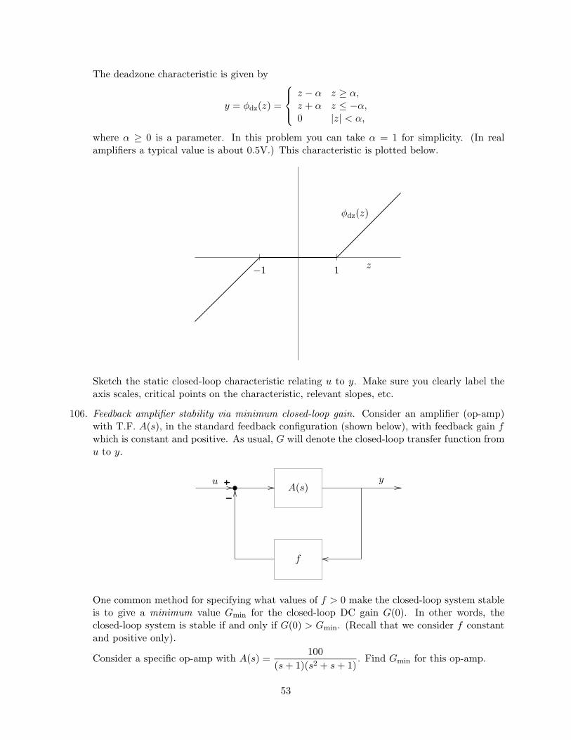
The deadzone characteristic is given by
y = φdz(z) =
z − α z ≥ α,z + α z ≤ −α,0 |z| < α,
where α ≥ 0 is a parameter. In this problem you can take α = 1 for simplicity. (In realamplifiers a typical value is about 0.5V.) This characteristic is plotted below.
z
φdz(z)
1−1
Sketch the static closed-loop characteristic relating u to y. Make sure you clearly label theaxis scales, critical points on the characteristic, relevant slopes, etc.
106. Feedback amplifier stability via minimum closed-loop gain. Consider an amplifier (op-amp)with T.F. A(s), in the standard feedback configuration (shown below), with feedback gain fwhich is constant and positive. As usual, G will denote the closed-loop transfer function fromu to y.
u yA(s)
f
One common method for specifying what values of f > 0 make the closed-loop system stableis to give a minimum value Gmin for the closed-loop DC gain G(0). In other words, theclosed-loop system is stable if and only if G(0) > Gmin. (Recall that we consider f constantand positive only).
Consider a specific op-amp with A(s) =100
(s + 1)(s2 + s + 1). Find Gmin for this op-amp.
53

107. A thermal system. A thermal model of the system shown below consists of outer shell, attemperature Tshell, which surrounds an inner core, at temperature Tcore. (Each of thesetemperatures is measured with respect to the ambient temperature.)
shell
coreqin
An external heat flow qin (in W) flows into the shell, and in addition there in a heat flowkshellTshell from the shell into the surroundings, where kshell is the thermal conductance be-tween the shell and the surroundings.
The heat flow from the shell into the core is denoted qcore, which is given by
qcore = kcore(Tshell − Tcore),
where kcore is the thermal conductance between the shell and the core.
The temperature of the shell satisfies
cshelldTshell
dt= qin − kshellTshell − qcore
where cshell is the heat capacity of the shell, and the right hand side is the net heat flow intothe shell.
The temperature of the core satisfies
ccoredTcore
dt= qcore,
where ccore is the heat capacity of the core.
For the remainder of this problem you can use the specific numerical values
ccore = cshell = 1, kcore = kshell = 1.
1a. Find the transfer function H from qin to Tcore. (Of course you can assume here that theinitial temperatures are both zero.)
1b. Suppose that the system starts with Tshell(0) = Tcore(0) = 0, qin(t) = 2000 for 0 ≤ t ≤0.001, and qin(t) = 0 for t > 0.001.
Find the maximum value of Tcore(t) for t ≥ 0.
You can make an approximation, but you must explain what you’re doing.
108. Stability range for feedback amplifier. An amplifier with transfer function A has a DC gainof 80dB, and three real, negative poles and no zeros. The dominant pole is at s = −100,and the two other poles are at s = −104 and s = −106, respectively. (This is a very typicalamplifier transfer function.)
54

2a. Find the unity-gain bandwidth of the amplifier, defined as the frequency for which themagnitude of the frequency response is equal to one. A good estimate is acceptable.
2b. The amplifier is connected in a standard feedback arrangement with feedback gain f ≥ 0,as shown below. Find the maximum value of f for which the closed-loop transfer function isstable.
A(s)
f
2c. Suppose the feedback gain f is chosen to be equal to the maximum value found in part b.At what frequency does the feedback amplifier oscillate? A good estimate is acceptable. Youmust explain your answer.
109. Driven guard. The figure below shows a common setup for an instrumentation system. Thevoltage source and resistance at left are the sensor; the resistance at right is the amplifier inputresistance. (We assume the amplifier output resistance is very low.) The voltage-controlledvoltage amplifier has gain a, which is positive.
The capacitance represents the capacitance from the wire connecting the sensor to the am-plifier to a shield or guard conductor around it. In a conventional arrangement, this shieldor guard conductor would just be grounded (and therefore, the bottom lead of the capacitorwould be grounded).
In this arrangement, the amplifier output drives the guard, and so it is called a driven guardsystem.
For this problem you can use the values
Rsensor = 100Ω, Ramp = 900Ω, C = 5nF
(which are quite typical).
For now, we’ll leave the gain a unspecified.
vsensor
voutv
C
Rsensor
Ramp av
iout
55

3a. Find the transfer function H from vsensor to vout. Please do this carefully as you mayneed to use it in the other parts of this problem.
3b. For what values of a is the transfer function H stable?
3c. Assume now a = 0.9. We define the response time of the system as the time it takesthe step response from vsensor to vout to settle to within 90% of its ultimate value. Find theresponse time.
3d. Still using the value a = 0.9, suppose the sensor voltage jumps from 0V to 0.1V. Whatis the maximum magnitude of the amplifier output current iout? (This value might be used,for example, to specify the output current capabilities of the amplifier.)
110. PD control. In lecture we studied proportional plus integral (PI) control. In this problem westudy proportional plus derivative (PD) control. PD control is also used in practice (but not asoften as PI control), often when a separate sensor is available that senses the derivative of theoutput, for example, a tachometer for a motor. A PD control system is usually implementedusing the block diagram shown below. The numbers kp and kd are design parameters (whichare usually, but not always, positive).
u yrP (s)kp
kds
We’ll study PD control applied to a DC motor, with transfer function
P (s) =1
s(s + 1).
4a. For what values of (kp, kd) is the closed-loop transfer function T (from r to y) stable?
4b. For what values of (kp, kd) are the poles of the transfer function T critically damped (andstable)? If no values of (kp, kd) yield critical damping, give your answer as ‘none’. If only onechoice works, give the specific values. If there are many choices, describe them all.
4c. Using the values kp = kd = 1, find the step response from r to u.
111. Transfer function synthesis from specifications. In this problem you will design a rationaltransfer function H from the followoing specifications:
• All the poles & zeros of H are real (to keep things simple).
• H has zero gain at DC and infinite frequency, i.e., H(0) = 0, and H(s) → 0 as s → ∞.
• H is stable.
56

• For ω between 101 and 103, |H(jω)| is 30 ± 3dB.
• For ω < 10−1, |H(jω)| is smaller than −6dB.
• For ω > 105, |H(jω)| is smaller than −6dB.
Use as few poles & zeros as possible to meet these specifications.
112. Design of multi-stage feedback amplifier. In this problem you will design a multi-stage am-plifier consisting of a number of cascaded stages, each of which is an amplifier of gain a witha feedback gain of f , as shown below.
a a
f f
u y
The amplifier gain a varies with temperature (say), over the range 40 ± 3dB (but you canassume that the gains in each of the stages are the same). The feedback gain f can beassumed certain; it does not vary with temperature.
You are to design the multistage amplifier subject to the specifications and objectives de-scribed below. Your final design will consist of the number of stages you use, along with thefeedback gain f used for each stage.
• Use as few stages as you can to meet all the specifications.
• The overall system gain (i.e., from u to y) must be 60dB within ±1dB, despite thevariation in the amplifier gain.
If you cannot meet the specifications using any number of stages, give your answer as ‘infea-sible’. You must justify your design.
113. Elmore delay of a convolution system. Consider a convolution system with impulse responseh and transfer function H. When h(t) ≥ 0 for all t, a useful measure of the delay induced bythe system is the Elmore delay, defined as
E(h) =∫ ∞0 th(t) dt∫ ∞0 h(t) dt
(provided the denominator isn’t zero).
(a) Express the Elmore delay E directly in terms of the transfer function H. Try to expressyour answer in as simple a form as possible. (Your answer cannot contain the impulseresponse h.)
(b) Find the Elmore delay of the following systems:
• a T -second delay• a first-order lowpass system with time constant T , i.e., transfer function 1/(1 + sT )• a T -second averager, i.e., y(t) = (1/T )
∫ T0 u(t − τ) dτ
57

(c) Elmore delay of a cascade connection. Suppose h and g are impulse responses for whichthe Elmore delay makes sense (i.e., h(t) ≥ 0 and g(t) ≥ 0 for all t, and the denominatorin the definition of Elmore delay doesn’t vanish). Let f = g∗h, i.e., the impulse responseof the cascade of the two systems. Are the following statements always true (i.e., truefor any g and h satisfying the conditions above)?
• E(f) ≥ E(g) + E(h), i.e., the Elmore delay of a cascade of two systems is always atleast as big as the sum of the Elmore delays of the systems.
• E(f) ≤ E(g) + E(h), i.e., the Elmore delay of a cascade of two systems is alwaysless than or equal to the sum of the Elmore delays of the systems.
If neither is always true give your answer as ‘neither’. You must justify your answer.We do not want conditions such as ‘E(f) ≥ E(g) + E(h) is true provided . . . ’.
58