EDUCATION FINANCE TRENDS IN A NO CHILD LEFT BEHIND AMERICA:

IMPLICATIONS OF STUDENT PERFORMANCE ON CHANGES IN PER-PUPIL SPENDING

A Thesissubmitted to the Faculty of the

Graduate School of Arts and Sciencesat Georgetown University

in partial fulfillment of the requirements for thedegree of

Master of Public Policy in the Georgetown Public Policy Institute

By

Ashley Branca, M.S. Ed.

Washington, DCApril 8, 2009

EDUCATION FINANCE TRENDS IN A NO CHILD LEFT BEHIND AMERICA:

IMPLICATIONS OF STUDENT PERFORMANCE ON CHANGES IN PER-PUPIL SPENDING

Ashley Branca, MS.Ed.

Thesis Advisor: Joydeep Roy, Ph.D.

ABSTRACT

The implementation of the No Child Left Behind Act of 2001 (NCLB) brought about

a new national system of high stakes accountability in which federal legislation, tied

to federal dollars, attaches student performance levels to severe, though graduated,

sanctions inviting stigma at both the district and school- levels. Given the federalist

structure of the education in the United States, state bodies have traditionally

controlled educational funding and school performance standards for their own

localities, with finance reform generally targeting cross-district equity. In order to

avoid the stigmas associated with failure on state standards tests, states may direct

aid to low-performing schools and districts. This study incorporates data for five

states, two of which have had pre-existing school finance reform. I use these data,

spanning from two years preceding NCLB until 2006, to assess whether or not a

significant correlations exists between student performance on standardized tests and

per-pupil spending, contributing to a potential explanation for differences in

ii

spending patterns after the implementation of the law. These evaluations are based

on state reporting of student performance and the department of education’s

Common Core of Data (CCD) documenting of per-pupil spending and enrollment by

district. Through the use of a fixed effects model within states over the course of the

time period selected, I find that overall there is not statically significant relationship

between per-pupil spending and student performance data, though there is a

statistically significance difference in spending across states with each progressive

year after the implementation of NCLB.

.

iii

Acknowledgements:I would like to thank my advisor, Joydeep Roy, for his continued assistance, insight, patience, and guidance throughout this oft-unforgiving process of writing my thesis.

I express great gratitude for all of my professors at Georgetown, specifically, Joe Ferrara, Lynn Ross, EJ Dionne, Jonathan Ladd, and lastly Harry Holzer, who helped me learn to love statistics. I have no way of adequately expressing my gratitude to Eric Gardner, who fielded my requests and dealt with my lunacy and shared great

music with me all hours of the day and night. I would also like to thank my parents, Tom and Donna, and my siblings, Colin, Adrienne, and Gianna, for their support throughout this and my other academic endeavors. I cannot overlook all of the support given to me by my best friend Kelly Florentino. Lastly, I would like to thank my friends here at Georgetown for listening to my endlessly babble, for

laughing at my jokes even when they are not funny, and for loving me anyway.

iv

Table of Content

Introduction……………………………………………………………………….....1

Research Design………………………………………………………………….…5

Design Rationale........................................................................................................12

Effect of No Child Left Behind Act on Spending Across States……………..…....15

Overall Trends......................................................................................................17

Understanding the Study Results…………………………………………………...19

Identifying Potential Explanations for Coefficients on Variables of Interest........22

Limitations of Study……………………………………………………………...29

Policy Implications………………..………………………………………….…..32

Conclusion……………………..……………………………………………….…...33

Appendix A-The Context of School Finance Reform………………………………37

Appendix B-Review of Previous Academic Literature…………………..…………42

Appendix C-State-by-State Regression Report…………………....……..…………50

Table 1- Michigan…………………………………………………………………...60

Table 2- Kentucky……………………...…………………………………………...61

Table 3- Florida……………………………...……………………………………...62

Table 4- Illinois…………………………....………………………………………...63

Table 5- Pennsylvania…………………………………………………………..…...64

Table 6- Overall………………………………………………………………...…...65

Table 7……………………………………………………………………….……...66

References…………………………………………………………………….……..67

v

Introduction

The dynamic federalist system of education in the United States has historically

led to great variation in quality of schooling across states, as each body holds authority

over decisions about educational systems within state, including testing and credit

requirements, accountability, certification, and fiscal programs. Consequently, school

finance reform has most often occurred at the state level, often based upon challenges

to the constitutionality of finance systems and ultimately intended to increase inter-

district fiscal equity. These attempts at reform have met with different outcomes and

varying levels of successfully changing state education finance structures.

No Child Left Behind Act of 2001 (NCLB), perhaps the most sweeping federal

program in the history of education in the United States, ties achievement on state

standards tests to state allotments of federal Title I funds and to a federal schedule of

sanctions and rewards. Because all states independently distribute these federal funds,

the impact of such distribution may differ across states; often mandated through

equity-targeted reform legislation, some states attempt to evenly distribute while others

may vary in uniformity, frequently due to finance formulas based on local property

taxes and values. Implementation of NCLB, a high-stakes law ordered by the federal

government but enforced at the state level, may promote a shift in focus from reforms

based upon equity to reforms targeting achievement.

1

While the system of education in the United States has enabled scholars to

readily undertake numerous state-level studies gauging the relationship between

spending and performance, the implementation of NCLB provides an interesting

opportunity to assess the effect of a universal federal policy treatment across states.

This paper evaluates the potential relationship between test proficiency and changes in

spending through the use of a state-level study hinging on the periods before and after

No Child Let Behind. Though these tests will evaluate differences within various

states over the given timeframe, such regressions, when applied to a range of localities,

allow for comparisons of the magnitudes and directions of results to draw conclusions

about the large-scale effects of the policy, differentiating between effects in states that

have implemented finance reform and those that have not.

The manifestation of these effects may reflect the historic context of funding

within states (see Appendix A for further elaboration). For example the ways that

finance reforms seeking to justify discrepancies in equity, such as those in Kentucky or

Michigan, have and will force states to adapt spending strategies in the wake of NCLB

may be statistically significantly different that the resulting differences in states

unaffected by finance reform and potentially exhibiting large variations in spending,

like Pennsylvania. Testing my hypothesis through a fixed effects model, I assess

variations in spending associated with student achievement from the two years

preceding NCLB to four years following and compare the magnitudes and directions of

2

results from within each state to the results uncovered across states. Such findings

could have great implications in explaining differences in spending, a traditionally

local responsibility, as a consequence of federal edict.

The figures used in the study come from both national and state sources. The

performance component of the dataset consists of aggregate and disaggregate

proficiency statistics for districts in the years before and after NCLB, with cohorts

broken down by grade, test subject, and proficiency levels to best target correlations in

spending. The data are recorded at the district-level, rather than at the school

proficiency level.

In order to ensure consistent reporting of finance data, the dataset includes

fiscal data for school years 2001-2006, collected from the United States Department of

Education’s National Center of Education Statistics, the Common Core of Data (CCD).

The fiscal data are reported in the form of per-pupil spending by district. Thus, the

measurement variables from the states and from CCD are both aggregated at the

district, rather than the school, level. These data span only the years 2001-2006

because of limitations in reporting; most states released test results from at least 2001

through the most recent testing, and CCD has released finance information only up to

and including the year 2006.

To best assess the potential relationship between altered financial distributions

and high-stakes testing performance levels after No Child Left Behind, the study

3

incorporates data from two states that had formerly implemented large-scale school

finance reforms, Michigan and Kentucky, and three that did not: Florida, Illinois, and

Pennsylvania. The selection of these states for the study occurred as a result of

numerous factors. First, theoretically, this paper seeks to analyze data from localities

that exhibit within-state variations in achievement and socio-economic levels. Four of

the five states in the sample are large and highly populated, with sizeable urban centers

that are ethnically and economically diverse. According to the American Legislative

Exchange Council’s 2007 Report Card on Education, these five are neither the highest

nor the lowest ranking states in the nation, with Pennsylvania, the highest standing of

the six, earning the 19th spot and Florida, the lowest, earning the 37th spot (LeFevre

1997). In theory, these states have the potential to show the greatest amount of

targeted change in spending given the large variance in achievement across districts

within.

The second major influence on inclusion of certain states is the quality of data

made available by the states. This paper will addresses the importance of data quality

in greater detail at a later point, but as it pertains to decisions regarding states at the

center of the study, performance data, collected from states, varied in consistency of

reported levels and in the number of years available across many states that could serve

this study, forcing them to be discounted as potential observations. This explains the

4

omission of such states as California and New York, two localities central to the

academic literature on school finance and effects of spending on student outcomes.

Research Design

This paper looks to account for differences in per-pupil spending after the

implementation of the No Child Left Behind Act of 2001 with the understanding that

this mandate brought about a high-stakes system of accountability that may have

caused states to target spending in low performing districts rather than focusing on

low-spending districts. Much of the academic literature expounding upon the

consequences of federal mandates on state fiscal policy and distribution suggests that

mandates seeking to improve student performance, at times through a more equitable

allotment of funds across districts as in the cases of Kentucky and Michigan, may or

may not correlate with a change in student performance (see Appendix B for further

elaboration). Adding to the field, this research tests the correlation between per-pupil

spending and student performance since 2001 under the assumption that some of these

changes might differ in states that have not already implemented sweeping finance

reform, and may have more room for changes in concentrated spending.

The No Child Left Behind Act of 2001 calls for schools within districts to meet

performance standards in order for states to receive federal funding. There is a great

deal of literature questioning whether money matters in affecting student performance,

5

much as there is an ongoing debate about the correlation between student performance

and other potential controls, such as class size and whether teachers have higher

degrees or not (Hanushek 1971, 1986, 1996). Undoubtedly, high and low performing

schools and districts have existed for as long as states have administered standardized

tests as a means of assessing knowledge, but after the authorization of NCLB, because

states must meet annual yearly progress in order to receive federal funding, the law has

higher stakes and may have a stronger correlation with attempts to improve test scores

through any number of levers, including per-pupil spending.

As noted, scholars, researchers, and educators hold mixed opinions as to

whether “money matters” in affecting student performance; high performance is

generally correlated with pre-existing high-socio economic factors, so achievement

may be the result of other factors. Simply increasing funds to already low-achieving

schools may not bring these schools to proficiency levels (Odden & Clune 1998)

(Rickman 1981). While the literature suggesting “money matters” in this regard is

neither highly significant nor highly robust, it does exist. Thus, when used properly,

increased funds, one of the few performance indicators that the government can

control, should have some (if minimal) positive effects on achievement.

Within this context, this paper assesses whether states without pre-existing

finance reform (those states in which spending might still not be equitable) are more

likely to increase spending in the lowest-performing districts in an attempt to increase

6

student achievement. Consequently, an increase in the change in per-pupil spending

would highly correlated to student performance by year. All vary in distribution of

achievement levels of districts within.

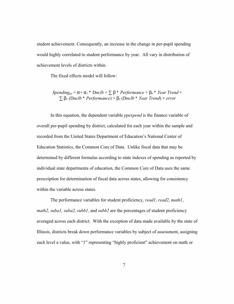
The fixed effects model will follow:

Spendingpp = α+ α1 ∗ Dnclb + ∑ β ∗ Performance + β0 ∗ Year Trend + ∑ β1 (Dnclb ∗ Performance) + β2 (Dnclb ∗ Year Trend) + error

In this equation, the dependent variable ppexpend is the finance variable of

overall per-pupil spending by district, calculated for each year within the sample and

recorded from the United States Department of Education’s National Center of

Education Statistics, the Common Core of Data. Unlike fiscal data that may be

determined by different formulas according to state indexes of spending as reported by

individual state departments of education, the Common Core of Data uses the same

prescription for determination of fiscal data across states, allowing for consistency

within the variable across states.

The performance variables for student proficiency, read1, read2, math1,

math2, suba1, suba2, subb1, and subb2 are the percentages of student proficiency

averaged across each district. With the exception of data made available by the state of

Illinois, districts break down performance variables by subject of assessment, assigning

each level a value, with “1” representing “highly proficient” achievement on math or

7

reading assessments and “2,” representing the student’s earning of “proficient” levels

on assessments as determined by each state. In this format, the analysis can assess

correlations and magnitudes on different achievement rankings. Additionally the data

in all states but Michigan includes these variables for the elementary, middle, and high

school grade levels, with each state specifying grades, from the 6 year period of 2001-

2006, allowing for specific assessment of targeted correlations.

This fixed effects model also uses a set of interactions between the student

achievement and NCLB dummy variable, nclb. Observations for the two years

preceding the implementation of NCLB, 2001 and 2002, are assigned the value of “0,”

and all other observations, comprising the “after” group, have a value of “1.” These

interactions account for the true effects of the treatment, controlling for otherwise

unintended corollaries. Furthermore, the trend variable accounts for each progressive

year in the sample, using 2001 as the base year. The inclusion of interaction terms

between the NCLB dummy, performance variables, and the ordered trend variable in

the regressions enables a clear assessment of the relationship between student

performance and per-pupil spending, as these values may vary per year. Otherwise,

without the inclusion of interaction terms, these changes might be conflated with other

effects in the model.

Lastly, the analysis includes results for data that are weighted and data that are

un-weighted, both by district enrollment. Through this process the study accounts for

8

the potential skewing of outcomes due to the variation in size between districts within

a state. Because states vary in the number of districts and the enrollment in each,

states’ financing formulas may also account for these differences. Since states reports

include results at the school, district, and state levels, it is important to account for the

ways in which the state accounts for district size in funding formulas. Because major

metropolitan areas often have higher enrollment numbers, these districts may garner a

greater percentage of overall funds, though their per-pupil expenditures may average

lower levels than spending in smaller districts. Additionally, weighting uncovers the

ways in which large district may be drive regression results. Without weighting the

data, each district is equal in the magnitude of its impact on per-pupil spending. Thus,

a comparison of both weighted and un-weighted results may provide a more accurate

picture of relationships between the dependent and independent variables.

I initially hypothesize that the magnitude of differences in spending accorded to

performance levels will be much greater for lower grade levels, as these students will

continue to undergo standardized testing for a number of years to follow, each

counting towards NCLB annual yearly progress (AYP) benchmarks. Thus, the

marginal returns to early investments will be much greater than those to later

investments, assuming spending increases learning and performance. Because No

Child Left Behind only calls for proficiency assessments in one year of high school,

9

districts may not necessarily increase funds to this group of students if increased funds

are, in fact, motivated by improving student outcomes on standardized tests.

On the other hand, accounting for the fact that most states only test one year in

high school, this test may garner a great deal of attention; with only one year’s and one

grade’s worth of data accounting for school-level AYP accountability, high schools

may be at a disadvantage, a fact for which districts may account through targeting

funds at the high school level. Either way, if my assertion holds true, district

performance could account for a great deal of the changes in per-pupil spending after

the implementation of No Child Left Behind because states will feel highly compelled

to target increased aid to low performing schools and most likely cap spending on high

performance districts.

The study utilizes short time series data in which NCLB serves as a “treatment”

marking a potential and long-lasting chance in the system. Cross-state finance systems

vary greatly, but within these locales, the general demographics, state economics, and

other population characteristics will not have changed within the time period at hand,

unless a dramatic shock to state or national institutions disrupts patterns of growth and

other stable characteristics. With the exception of the treatment of No Child Left

Behind, the population within the state will not have altered, and all characteristics and

unobservable (but unchanging) qualities drop out of the panel when we run the

regression across years. The importance of the fixed effects regression, then, is to

10

account for large within state variation. Because the states in the sample may differ

greatly from one border to the other, a fixed effects model will answer for such

heterogeneity, averaging effects across the states for each year. Notably, this model

has the ability to specifically account for other important factors that might affect

spending and achievement. Accounting for characteristics that might otherwise shape

results, like the ethnic make-up of the population, social structures and contexts, and

the locale’s economic profile, the fixed effects model averages characteristic means of

the entire population across districts.

The primary variable of interest in this testing is that of per-pupil expenditure,

ppexpend, which is the total outlay per student in any given district. The study uses this

variable to assess correlations between student performance and spending, specifically

focusing on whether low proficiency levels in test scores will be directly correlated

with an increases in per-pupil spending and whether high-performing districts will

otherwise not see increases in this manner. Though it is not obvious that additional

money will help induce better performance, spending is one of the few instruments at

districts’ disposals to potentially influence outcomes. Consequently, some states may

have determined that money does not have strong effects on student achievement and

that they cannot change outcomes through adjustments in spending patterns. Others

might determine the opposite, reacting by re-allocating resources to best target areas in

need of improved achievement levels. In some ways, this potential for change is

11

dependent on the fact that these divergent levels have historically existed and persisted

despite various attempts to close achievement gaps.

It is essential to recognize that this study may contain a certain level of

ambiguity in results: if test scores rise with an increase in per-pupil spending but still

remain below proficiency levels, administrators might seek to continue this trend the

following year or until students reach proficiency. This pattern might materialize in the

form of a positive correlation between test scores and per-pupil spending at certain

levels. This study is limited in its ability to differentiate between these two effects.

Design Rationale:

Many papers look at the intersection of school finances and state testing results

to assess the effects of spending on student performance. The opposing theoretical

question would be to assess how student performance might intersect with finance in a

way that proficiency levels affect finance decisions. Specifically, one might ask how

might policymakers use testing data to make decisions about where they will change

spending levels in order to affect future achievement? If one can assert that

inconsistent fiscal distribution perpetuates the systematic, academic acceleration of

certain groups while hindering the performance of others, it follows that NCLB

encourages states to adjust distributions as a remedy for performance shortfalls.

However, if a state had previously adjusted spending in the hopes of equitably

12

addressing performance concerns, this locality may not feel the need to alter finance

formulas in a post NCLB environment.

The presence of such pre-existing finance reform alone, however, might not

account for changes in per-pupil spending. For example, research in some states has

shown that funding systems reliant on garnering revenue mostly from local taxes, often

including property and income taxes as well as other non-property taxes, tend to have

overall higher per-pupil spending than those bodies whose finance structure is

comprised of a state-centered and run funding system through, perhaps, sales taxes. If

finance formulas affect per-pupil spending, these systems may correlate to changes in

per-pupil spending and achievement over the years at hand.

The research behind this analysis has been guided by the theory that the No

Child Left Behind Act raised the stakes for performance, and since fiscal policy is one

lever that is often used in an attempt to increase performance (as measured by

proficiency in conjunction with other factors, including completion, attendance,

graduation rate, etc), states would adjust spending in the areas most in need of

increased assistance to reach proficiency, ideally yielding long-term benefits for state

education agencies.

Following the same logic, states may be more inclined to focus fiscal increases

in per-pupil spending on younger grades because early intervention can yield much

higher marginal returns for each dollar. Essentially, as students advance in grade, the

13

number of times they will be tested and affect annual yearly progress decreases. Thus,

each dollar spent on a pupil in an effort to enhance achievement has diminishing

marginal returns with every increasing year. Consequently, school districts might be

more likely to disproportionately fund early grades and decrease funding to each year

because the number of tests each student faces continues to decrease each year, so

investments in upper-level grade will not have high returns.

It is possible that low-spending districts may not be low-performing districts.

While under-resourced areas may disproportionately underachieve, the existence of

equalized but low spending across states that demonstrate variation in achievement

bolsters arguments suggesting that other characteristics and factors may significantly

affect achievement. That said, if certain low-spending areas still attain higher

achievement levels, given that fiscal resources are one of the few mechanisms that

policy-makers can adjust, then it follows that states might be more apt to increase fiscal

levels to certain low-performance districts over others rather than increasing funds

across the state. The validity of this assertion hinges on the educational context,

created by NCLB, in which testing results have the high stakes of not only affecting

federal funding levels but also of stigmatizing failing schools and districts. If sanctions

do not pose a suitable threat to states, there may be little reason to think local

government will change any behaviors in the hopes of improving performance.

14

In assessing expected results, one cannot ignore the tendency for general

increases in spending over time, whether these changes are spurred by government

mandate or not. Given the systematic boost in per-pupil spending over the years

within this study, I believe that there will be an insignificant and positive correlation

between time variables and per-pupil spending. Because of an emphasis on early

intervention in education, however, I ultimately expect there to be negative and

significant relationship between elementary grade-level achievement and expenditures,

with similar patterns for coefficients on high school performance. For reasons already

discussed, however, the direction of this coefficient may go in the opposite direction.

Effects of No Child Left Behind Act on Spending Across States

In this study, regressions across states exhibit results of similar significance

levels on many of the same variables. These results suggest that there is not a

statistically significant difference in spending as a result of student performance after

the implementation of No Child Left Behind, thought most states exhibit statistically

significant differences in spending with each progressive year after this treatment. The

results disprove the initial hypothesis stating states that had previously implemented

finance reform may have sought to address variation in district spending and any

associated student performance and might be less likely to adjust spending patterns

after 2003, when the high-stakes testing component of NCLB actually began.

15

Across these finance reform states, regressions results varied. Though both

revealed significant correlations between spending and the time data, particularly in the

post-NCLB period, the coefficients on the nclb*trend variable for the Michigan

regressions had a negative sign (see Table 1), while the coefficients on the same

variable for Kentucky had a positive sign (see Table 2). Both states also have scattered

significance on inconsistent performance variables in the post-NCLB period, and the

inconsistencies in these results suggest that they could have occurred by chance. These

results hold true for the overall regressions.

The paper had asserted that states not previously employing measures of

finance reform might be more likely to adjust spending patterns after the treatment of

No Child Left Behind. As such, differences in financial allotments may correspond

with district performance, as states use proficiency levels to target modifications in

spending. Again, the results disprove the initial hypothesis and show similar trends as

those for the regressions in finance reform states. The results for Florida (see Table 3)

resemble outcomes for Kentucky, with scattered significance on performance variables

and positive, highly statistically significant coefficients on the nclb*trend variable.

Both Illinois (Table 4) and Pennsylvania (Table 5) demonstrate statistical significance

on this variable, though the coefficients go in the negative direction. Unlike the other

states in the sample, Illinois shows no statistically significant coefficients for post-

16

NCLB performance, suggesting that such correlations did not even occur by chance in

this sample data.

Overall Trends:

Though the magnitudes and significances of the coefficients on performance

variables differed across grades and states, the trend across all states and grades was

the significance of coefficients on nclb, trend, and nclb∗trend. Though the coefficients

on nclb and trend had mostly positive signs, the interaction term nclb∗trend often

exhibited a highly significant and negative coefficient. This relationship suggests that

though per-pupil expenditures may increase in the years following no child left behind,

these expenditures vary across districts and the varied results cause a negative overall

correlation.

Table 6 shows the weighted and un-weighted results for pooled data regressed

across all years and grades for each state. This table demonstrates that across all states,

there is a highly statistically significant correlation between per-pupil expenditures and

each increasing year after the implementation of No child Left Behind. The

coefficients vary in size and direction, as Florida and Kentucky, one state that had

previously implemented sweeping school finance reform and another that had not,

demonstrate significant and positive coefficients on this variable, while the other states

in the study show significant and negative results.

17

These results may correspond with the fact that both Florida and Kentucky are

comprised of a small number of large school district, perhaps contributing to less

variation in spending across district. This kind of distribution would allow overall

increases in spending to be reflected as positive coefficients, given that such an

absolute increase in spending would correspond to a district increase in spending,

whereas in states containing many school districts will show an overall increase in

funds, but the rates of increase will vary and perhaps occur at a decreasing rate.

In addition to the universally significant nclb variable, both nclb and trend are

highly significant and positive in almost all regressions. This result reflects the

disaggregated regressions discussed above, and is what we would expect of state

results. Table 7 shows the percentage differences of change in per-pupil expenditures

associated with these three variables, as obtained through logging the dependent

variable. This table charts changes in the context of overall spending, an important

exercise given that spending differs greatly across state given local costs of living and

wages. When logging the variable, the results are highly significant, and as in the Table

6, the coefficients on nclb∗trend for Kentucky and Florida are negative.

Finally, Table 7 shows that with the exception of the results for Florida and

Pennsylvania, the percent change in per-pupil expenditure associated with nclb and

trend across states tends be in the same range. These changes in Florida average two

percentage points lower than most states, while the results in Pennsylvania are the

18

same or two percentage points higher than the rest of the sates. Interestingly, the

change associated with nclb∗trend in Florida is an increase of 5% of per-pupil

expenditures. The other states are similar in absolute value of change, though the

direction of these results in inconsistent across states, perhaps for reasons explained in

analyses of individual states.

Consistent with assessment of individual state results, the analysis of all data

disprove my initial hypothesis that states who had not previously implemented school

finance reform would be likely to adjust spending after the implementation of No Child

Left Behind, reflected in a significant correlation between student performance and

per-pupil expenditures. Across all states, correlations between performance data and

spending after No Child Left Behind were not statistically significant. Even more

telling is that the variables that did exhibit highly significant coefficients were

consistent across states, independent of former finance reforms.

Understanding the Study Results

As noted, the regression analysis results disprove my initial hypothesis that

states who had not previously implemented school finance reform would be likely to

adjust spending after the implementation of No Child Left Behind, reflected in the

regression as a significant correlation between student performance and per-pupil

expenditures. The inter-and-cross state variation in significance and direction of

19

correlations between performance and per-pupil spending suggests that the effects of

the law differ from state to state but with no discernable relationship with the

occurrence of pre-existing state finance reform. Furthermore, the haphazard

occurrence of significance in the coefficients on performance variables suggests that

there is no distinguishable pattern in the relationship between student achievement and

spending across or within states. Thus, such significant relationships may occur by

chance, rather than by volition.

Despite differences in the relationship between spending and performance, on

the whole, nclb, trend, and nclb*trend were highly statistically significantly correlated

with per-pupil spending. Independently with each increasing year and in the period

after the implementation of NCLB, per-pupil expenditures increased in overall

magnitude. As expected, looking at the pooled data, with the exception of results for

Kentucky, nclb and trend both exhibit positive and highly significant coefficients.

This results is as expected; as noted in the introduction, even without the treatment of

No Child Left Behind, spending on education has steadily increased over time, though

these increases may in part reflect changes in the value of the dollar over time.

Surprisingly the direction of coefficient on variable most frequently significant,

nclb*trend, was inconsistent across, and at times within, states; regressions yielded

positive coefficients on this variable in Kentucky and Florida and negative coefficients

in Michigan, Illinois, and Pennsylvania. The paper will address the implications of this

20

findings in the next section, but in terms of the interpretation, one might conclude, that,

as expected, these correlations are significant given the changes in spending over time

compounded with changes in spending associated with fund attached to NCLB.

Of particular note are the findings for the state of Florida. The logged

regressions for this state yielded the smallest percent change on trend, with magnitudes

of 1% and 2% (weighted), the smallest percent change on nclb, with 2%(weighted and

un-weighted), and the largest percent change on nclb*trend with 5% (weighted and un-

weighted). These results may reflect state system characteristics, as Florida has the

fewest school districts of any state in the sample with 67 total, one for each county.

This likely means each district has a high enrollment, and there may be little significant

variation in these numbers for districts across the state. Additionally, other

characteristic data may average out across these large districts.

Perhaps for opposite reasons, Pennsylvania exhibits the largest change in per-

pupil spending after NCLB, with a change on the magnitudes of 9% and 10%

(weighted). This may be the result of an overall increase in spending across the state,

given that Pennsylvania is comprised of many districts that vary in enrollment,

spending, and achievement. This great variability may allow dramatic increases in

funds allotted to the lowest spending districts to disproportionately determine the

magnitude of results.

21

Overall, variables that did exhibit highly significant coefficients were

consistent across states, independent of former finance reforms. Trends in the results

seem to reflect state district compositions, independent of finance or NCLB legislation.

These trends may also reflect the number of failing schools within a district, a level of

analysis not present in this study. The assertion here is that states that have a small

number of failing schools may not consider failure under NCLB to be a realistic threat

and may consequently respond or neglect to respond to individual school failure. Even

more significant than the absence of a pattern along the lines of pre-existing finance

reform is the overall dearth of significant correlations between spending and

performance after the implementation of No Child Left Behind. The following section

provides plausible explanations for these effects or absence thereof.

Identifying Potential Explanations for Coefficients on Variables of Interest:

The passing of NCLB opened a potential policy window that would allow state

policymakers to adjust spending patterns in order to target fiscal increases to the lowest

performing schools. The data collected and analyzed in this study show, however, that

for the 5 states incorporated into this study, there is no statistically significant

correlation between student performance and spending in the years following the

institution of NCLB. At the same time, though most results reveal an increase in

spending in each progressive year in the study and in the period after NCLB, an

assessment of the relationship between per-pupil spending and each progressive year

22

after NCLB shows that this relationship, while highly statistically significant, is

inconsistent in direction. A number of dynamic factors may serves as credible

explanations for these results.

1. Changes to the test:

In some cases well before the passage of NCLB, all the states in this study had

previously developed and begun to administer state standardized tests by which to

assess student proficiency levels1. Though not yet mandated by federal law, states

oversaw these assessments to gain a better understanding of student mastery on

standards-based content. Thus, by the time President George W. Bush signed NCLB

into law, requiring that each state draft standards and test accordingly, most states

already had a few years head start in experience in this undertaking.

In first two years following NCLB however, many states applied to the US

Department of Education for approval on proposed adjustments to guidelines laid out

in state accountability workbooks. Most of these applications sought departmental

permission to change the levels and content of tests used to determine states’ annual

yearly progress. A number of these changes directly corresponded with adjustments

that states had already made to their standards. Additionally, some states sought to

1 State abbreviation followed by first year is state test administration follows: MI(1997), KY(1999), FL(2001), IL(1999), PA(2001) Source: CCSSO, “State Education Indicators With a Focus on Title I 2002-03.” US Department of Education (July, 2007). Retrieved March 2009: http://www.ed.gov/about/offices/list/opepd/reports.html.

23

change definitions of proficiency, adjusting (i.e. lowering) the level at which students

had to achieve in order to be counted as proficient or above. Within this context, some

states sought approval to gradually increase proficiency requirements.

On the mechanical side of test administration, some states had to adjust the

grade levels and number of proficiency levels they reported. No Child left Behind

requires that states administer and report results from at least three grades, each at a

different level: elementary, middle, or high school. As prior to NCLB not all states

had tested and released data in this fashion, numerous entities applied for permission to

adjust the grades counted towards annual yearly progress and their associated

assessments (US Department of Education 2007).

In an even greater divergence from previous test records, some states, including

Florida in 2006, sought permission to move towards a value-add system of

accountability, known in the testing context as a “growth model.” This method for

determining proficiency measures student growth against prior year achievement rather

than measuring cohorts for the same grade in each consecutive year. This model looks

at student improvement rather than absolute achievement in order to gauge progress.

Consequently, all of these changes essentially nullify the impact of past results,

with states likely to discount achievement level prior to these adjustments. Due to

changes in tests and accountability plans, states may not count previous years’

performance data as truly reflecting proficiency. Such disregard may cause states to

24

delay or altogether neglect to adjust spending as a result of performance before

assessing results after administering new tests.

2: Weak enforcement of sanctions:

Without question, the most divisive component of the NCLB mandate is the

system of sanctions that accompany student achievement. The law requires that each

state abide by a specific timetable for the implementation of these injunctions, but it

does not determine how states hold districts accountable or how they determine the

failures and successes of schools and districts. Per the specified timetable, schools not

meeting annual yearly progress targets for two years in a row do not face sanctions,

only earning the label of being a failing school, the stigmatizing effects of which could

serve as the focus of a separate and detailed paper. Given this schedule, it is only in the

third consecutive year of failure in which schools face negative sanctions. These come

in the form of requiring the school to write a school improvement plan and offering

school choice to all students.

With each consecutive year of failure, punishments associated with no Child let

behind progressively increase in consequence, eventually leading to the restructuring

of schools. Importantly, states measure annual yearly progress at both the school and

district levels, with similar graduated consequences. Yet, like school level sanctions,

these consequences only take effect in the 3rd consecutive year of failure, in the case of

25

this study, the second to last sample year, and 2006. Even then, the magnitude of

consequences is not great.

Additionally, these sanctions very in magnitude and effectiveness of

implementation across states and districts. When they imposed NCLB mandates

during the early stages of NCLB included in this study, states did so with differing

levels of efficiency, strictness, and overall guidance. While some states and districts

stringently imposed sanctions others focused more on other interventions (Manna

2007). Because districts can average scores across all schools, rather than focusing on

sanctions for failing schools, it is quite possible that they allowed high achieving

schools to unduly drive perceptions of progress. Soft and inconsistent enforcement of

sanctions may have built confusion around the true requirements of the law.

Few can doubt that many triumphs and failures associated with No Child Left

Behind hinge on the successful application of the system of sanctions laid out in the

Act (Hess and Finn 2007). Thus, it is highly possible that given the graduated nature

of NCLB sanctions and due to the fact that the last year of our sample was only the

first year in which schools entered corrective action, for the length of time allotted to

the data in this study, schools and districts alike did not feel the pressure of or high

stakes associated with NCLB. Consequently localities would not restructure spending

patterns in the hopes of improving performance because they did not feel the urgent

26

need to do so; the sanctions associated with NCLB simply did not pose a significant

threat on the horizon for most schools.

3: Not enough years in sample:

The study may not have spanned enough years to allow for a true assessment of

the effects that NCLB will have on the relationship between spending and achievement

in a post-law period. Given the magnitude of policy and number of administrative and

technical changes that occurred in the early stages of implementation, there is reason to

believe that no great modifications to finance patterns would occur within the four-year

post-NCLB period included in the data. Thus there may not be enough years in the

sample to truly assess how performance data will correlate to per-pupil spending and

whether these relationships will look significantly different in states that had pre-

existing finance reform as compared to those who have not.

This finding may be further bolstered by the fact that over the time period

included in this study, numerous states, including some within the sample, took steps

towards appropriately adjusting fiscal policies in the next few years. Some states have

and are commissioning costing-out studies (as noted in Appendix B) while others are

looking into voucher programs that may change distributional policies altogether.

4. Need to redirect funds to other areas:

Though NCLB increased federal aid to states, it also amplified cost burdens in

the undertaking of administration, data systems, training, test creation, implementation,

27

and distribution of information. Arguably, states need to frontload efforts in these

areas to establish accountability systems that will yield long-term success. As a matter

of necessity, then, states may have used newly distributed NCLB funds to improve

NCLB structures. Thus, it is possible that the states could not target spending

according to performance because, in the early stages of the law, they had to focus

monies in other areas. This area could warrant additional research.

5. Focus on other levers to make AYP:

Student Performance is not the only area upon which schools and districts need

to improve in order to make AYP. Schools also had to improve sub-group student

achievement and participation, overall test participation, student attendance, graduation

rates, teacher quality, and access to advanced placement and college preparatory

classes. Because development of high-level course offerings and programs to increase

test participation and overall student attendance may prove to be more reachable

targets, regions may choose to focus fiscal efforts on the bolstering of these programs.

It is possible that districts further prioritized the improvement of other levers based

upon knowledge that state testing was in nascent stages, as supported by the large

number of test revision approvals submitted to the Department of Education.

6. Inability to rapidly change finances at the local level:

Budget and finance reform decisions occur through a complicated process

occurring at many levels. Increases in funds at one level do not necessarily change

28

finance formulas at another. An increase is state aid may have minimal influence on

differences in budget changes; though changes in supply might warrant adjustments to

local fiscal policies, these increases do not necessarily correlate in successful budget-

altering votes (Ehrenberg et al. 2004). The implication, therefore, is that many political

and bureaucratic factors affect fiscal policy decisions, making the act of changing these

policies more difficult. As a corollary, though NCLB increased federal funds flowing

to states through Title I monies, these fiscal escalations did not necessarily translate

into directed budget changes at the local level. Thus, even if state policymakers sought

to target funds after NCLB, they may not have been able to do so.

7. States don’t believe that spending correlates to achievement:

Lastly, given that some academic literature shows strong and statistically

significant correlations between spending and increased achievement, others show the

opposite. It is quite possible that states, aware of this mixed support that does not

definitively support positive effects, chose not to target spending as a lever for

increased achievement.

Limitations of Study:

Though it generated statistically significant results in variables associated with

time effects on spending, the study has many limitations, many of which directly

correlate data availability and quality. Additionally, the study suffers from the threat

29

of endogeneity bias, though the absence of significant correlations between per-pupil

spending and student performance minimizes the consequence of this potential hazard.

The problems with the data used in the study are manifold. First, the data only

spans a limited number of states over a small number of years. While the data are

consistent in these time periods across states, the length of time assessed may

adversely affect the robustness of results. The data are a product of reports made

available by the states and from CCD, as the national core databank only released

finance data through the 2005-2006 school year, a two-year lag from the date of

submission for this thesis. Also, while some states released testing results for years

prior to 2001, to maintain consistency across the sample, this data includes

performance data from the earliest common year, in this case 2001, the year Florida

and Pennsylvania developed official state standards tests. The need to maintain

consistency in this way limits the data in that the number of years applied to the “pre-

NCLB” period is half the size in the “post-NCLB” period, which in and of itself only

extends over four years.

The study is also limited in that state data are inconsistent in content and

reporting across localities. Though after 2003 all of the states report consistently by

grade, proficiency levels, and subjects, prior to this point, the data are variable, often

for reasons explained in analyses in previous sections of this paper. For example,

though NCLB mandates that state test and report at the elementary, middle, and high

30

school grades, the Michigan Department of Education does not post pre-2003 test

results for the high school level. As a result, no high school grade is present in the

Michigan data. This lack in consistency casts doubt upon the strength and validity of

the dataset employed in this study, and consequently of the results found herein.

Data inconsistencies in reporting, both in terms of the variables and levels of

interest as well as the format of these releases, limited the number of states that could

be included in the study. While such large states as California, New York, and Texas

would have provided interesting and compelling data to enhance the work in this

paper, data limitations and lack of resources restricted the actual number of states

assessed. Variability in the tests utilized to measure AYP, as in the case of Texas,

condensed the potential pool of states from which to draw data for analyses.

Lastly, an additional limitation of this study is the potential threat of

endogeneity bias that exists in the data. This bias may exist between per-pupil

spending and student performance. Essentially, because this is a natural and not

constructed experiment, without the use of an instrument, there is no method by which

one can determine one-way causation between changes in student performance and

increases or decreases in per-pupil spending. It is quite possible that changes in student

performance can cause change in per-pupil spending. On the other hand, it is equally

possible, as noted in the literature review, that changes in spending may affect changes

in student performance. Only the replication of this study in a constructed manner or

31

the utilization of an instrument could allow for the isolation of effects of student

performance on changes in spending. Otherwise, one must note that correlation does

not necessarily reflect causation.

Policy Implications:

Though the previously discussed limitations may restrict the policy

implications of this study, the findings in this paper may still shed some light on

legislation associated with No Child Left Behind and other federal and state mandates.

First, these findings may suggest that the NCLB mandate, while written with

the intent to provide states that fail to meet annual yearly progress with ample

opportunity to repair failing schools, the sanctions associated with the mandate may be

too soft to spur real change. Policymakers may want to assess the effectiveness of

specific sanctions and scales to improvement across the graduated scale of

consequences. Perhaps in reauthorization, lawmakers might truncate the sanction scale

or shift priorities of consequences.

As a corollary to the limitations of this paper, with respect to reporting

requirements, the undertaking of this study suggests that the federal government should

serve as a hub for the compilation of state data. Federal law could mandate that states

report student performance results, still state-defined and reported, to a central

database. This would facilitate easier and more thorough assessments of federal and

32

state education programs, bolstering the wealth of information on education program

evaluations.

While this paper does not advocate federal regulations mandating the targeting

of fiscal increases to the lowest performing districts to the exclusion of already-high

performing districts, it does acknowledge that this could be a potential area for policy

exploration.

Conclusion

This study finds no statistically significant correlation between per-pupil

spending and performance in the year following the implementation of No Child Left

Behind, illuminating the lack of differences between states that have and have not

undertaken large-scale education finance reform. This study incorporates data for five

states, two that have had pre-existing school finance reform. Through the use of a fixed

effects model within states over the course of the time period selected, I find that while

there is not a statistically significant correlation between student proficiency and

spending, there is a statistically significance difference in spending across states with

each progressive year after the implementation of NCLB. The magnitudes and

directions of these differences vary across state and demonstrate no discernable pattern

finance reform versus non-finance reform states.

33

As with many academic works, this paper, limited in content and constricted by

timeframe, serves as the first step in an iterative process of program evaluation. First,

the results of this paper lend support for the continuation of this study in future years

and across a larger sample of states. The expansion of the data in this method would

allow for greater confidence in true effects of the relationships between the regression

variables. Additionally, as the policy context of education continues to change, this

study supports the continued evaluation of the relationship between modifications in

spending and their potential educational outcomes. Importantly, this continued

research would be best focused in constructed experiments designed to assess

causation between the two variables, eliminating the potential for endogeneity bias.

Another area for further research emerging as a result of this study would be

extended assessment of the varied but highly significant coefficients on the nclb*trend

variable. Checks for robustness through dropping highest enrollment districts in four

of the five states in the study did not affect the significance of this variable across

states, as might be expected, but these checks did alter magnitudes of coefficients,

particularly in the weighted regressions. In non-finance reform states Illinois and

Pennsylvania, previously negative coefficients on nclb*trend were more negative after

dropping Chicago and Philadelphia respectively. The finance-reform states, Michigan

and Kentucky, demonstrated opposite results when dropping largest school districts, as

absolute values of magnitudes on the nclb*trend coefficients decreased. Importantly,

34

states with the smallest number of districts (and thus the most consistently high

enrollment districts) did not exhibit large-scale changes in these checks2. Further

analysis of this relationship is warranted.

As states move towards new models for assessing proficiency, such as through

a value-add or growth model, future studies should consider the ways in which these

new barometers correlate with spending and whether such changes vary over the

course of a significant number of years. Furthermore, the study warrants future

research utilizing lagged data and assessing whether the effects of the treatment exist

as theorized but only emerge multiple years after the release of test results. This is a

significant possibility given that the magnitude and high stakes associated with the test

often cause lags in the release of results, potentially skewing the possibility for

localities to make informed fiscal decisions or to propose budgetary changes.

Lastly, the next step in this process may be to refine the variables used in the

analysis. The dependent variable in this regression, per-pupil expenditures, is the

overall level of spending by student. Perhaps the variable of greatest interest for an

analysis of effects of student performance on changes in spending is the value of state

aid going to particular districts. While per-pupil expenditures reflect overall spending,

state-aid reveals assistance given to districts over and above baseline spending. This

2 In Illinois, dropping Chicago: weighted nclb*trend = -378, unweighted nclb*trend= -450; Pennsylvania, dropping Philadelphia: weighted nclb*trend = -233, unweighted nclb*trend= -274; Michigan, dropping Detroit: weighted nclb*trend= -174, unweighted nclb*trend= -280 Kentucky, dropping Jefferson County: weighted nclb*trend = 80, unweighted nclb*trend= 130. Florida counties approximated the same size, so no observations dropped.

35

variable may provide a more accurate sense of targeted spending as this may currently

be masked in the regressions of overall expenditures.

36

Appendix A: The Context of School Finance Reform

Outside of the No Child Left Behind Act of 2001, few federal laws have sought

to intervene in states’ educational platforms, and, consequently, the genesis of school

finance reforms has differed from state to state. In some instances finance reform

occurs as a result of lawsuits brought against the locality by individuals or interest

groups. In their arguments, these bodies often argue that state finance systems

demonstrating large spending disparities across districts are unconstitutional,

discriminatory, and remiss.

These cases had various outcomes. The 1971 case of Serrano v. Priest

(Serrano II) brought forth accusations that California’s education finance system

disproportionately benefited wealthy students and neglected those students of lower

income levels, many who were minorities and recent immigrants. The California

Supreme Court’s ruling affirmed lower court findings that wealth-related disparities in

per-pupil spending generated by the state's education finance system violated the equal

protection clause of the California constitution. This case led to reforms centralizing

spending in an attempt to eliminate cross-district inequalities.

Plaintiffs in Kentucky, one of the five states included in this study, had similar

successes through legislation mandated by the 1988 decision in the case of Rose v.

Council for Better Education. In this case, a coalition of school districts argued that

the state’s system of education finance violated a constitutional clause mandating that

37

the “General Assembly shall, by appropriate legislation, provide for an efficient system

of common schools across the state” (Adams 1997). Convincing the court that

Kentucky had not ensured the right for children to obtain an “adequate education,” the

plaintiffs saw state officials overhaul the education funding and tax structures in order

to reduce cross state inequity and to raise overall spending. Interestingly, the new state

legislation also included requirements for standardized testing and accountability.

In a counter example, similar suits in Pennsylvania, one of the states in this

study, yielded very dissimilar results. Despite hearing at least 3 cases challenging the

constitutionality of it school finance system (Danson v. Casey (1979), Marrero v.

Commonwealth and Pennsylvania Association of Rural and Small Schools v. Ridge

(1998)), the Pennsylvania Supreme Court has consistently held that because funding

decisions are specifically the responsibility of the legislative branch of government, the

court should not decide upon lawsuits against the commonwealth’s public school

funding system. The consistent upholding of this decision maintains a funding system

based heavily on local revenues as established by varying tax systems within each

locality. Consequently, cross-district discrepancies in per-pupil spending still exist in

this state.

Similar logic has held in both Illinois and Florida, the two additional non-

finance reform states in this study. In the case of Committee for Education Rights v.

Edgar (1996), the Illinois Supreme Court faced a question of whether the state’s

38

disproportionate reliance on local property taxes as the main source of revenue for

public schools perpetuated a system in which the poorest districts did not have

adequate funding and equal access to education as defined by the state constitution.

Acknowledging that cross-district disparities were great, the Illinois Supreme Court

argued that the constitution did not define “adequacy,” and because such finance

decisions were the responsibility of legislators, the court would not decide on the case.

The courts upheld this decision in Lewis E. v. Spagnolo (1999). Undertaking a costing

out study in 2000, Illinois has since increased the overall levels of spending at the state

level, though distribution and collection of resources still occurs at a local level.

Per the implications of the Illinois rulings, lawsuits are not the only methods

through which finance reform has occurred, as numerous states enact reforms by way

of ballot referendums through which citizens can vote to affect state finance policies.

One such example is Michigan’s 1994 passage of Proposition A. This governor-led

legislation centralized spending at the state-level and eliminated the use of property

and local taxes for education revenues, adapting a finance system in which educational

funding oems from state sales taxes. Thus, Michigan found a way to centralize

spending in order to increase resources to lower-income areas while limiting any

increases in spending to already high-resources districts.

Also raising issues over adequacy of funding, in the 1995 Florida Supreme

Court case Coalition for Adequacy and Fairness in School Funding v. Chiles, the

39

plaintiffs argued against the state’s system of resource allocation. Florida rulings

echoed precedent set in Committee for Education Rights v. Edgar, as both high and

low courts struck down the case, stating that plaintiffs had not convinced the courts

with a definition of adequacy that would impel judicial intervention into the legislative

process, as this could prove destructive. Consequently in a 1998 state-led initiative,

Florida voters approved a referendum altering and clarifying the language of the state

constitution. Subsequent cases have failed to bring forth large-scale state education

finance reform, though Florida has experimented with other initiatives, including

school-choice based programs. Essentially, however, Florida courts argue that such

fiscal policymaking must happen in the halls of the capitol rather than the courtroom.

In all, lawsuits challenging the public funding of schools have been brought

forth in 45 of the nation’s 50 states3, with litigation leading to reforms in two of the six

states at the center of this study, Kentucky and Michigan, but not in three others,

Pennsylvania, Florida, and Illinois. However, the absence of such rulings has not

precluded states from conducting “costing out” studies to gauge adequate levels of

spending across districts (Powers 2004), nor does a ruling deeming funding systems

unconstitutional, inadequate, or inequitable lead to actual reform. For example, though

the 1982 decision of Levittown v. Nyquist, 439 N.E.2d 359 determined that the New

York state constitution guarantees students the opportunity for a “sound basic

3 From National Access Network. http://www.schoolfunding.info/litigation/litigation.php3 (accessed 12/16/2008)

40

education,” and great inequities existed across districts within the state, legislators only

began to plan for finance reform after the 2001 decision of CFE vs. New York State.

This decision, ultimately upheld through the appeals process, charged the state with

determining the appropriate levels of funding through which students are ensured

access to educational opportunities no matter their socio-economic background. Yet,

as of 2006, no real change in finance had occurred. Putting into action a costing out

study, this reform targeted adequacy and not equity, a shift in approach from other

plans that sought to equalize spending across districts. Importantly, the reforms place

budgeting control in the hands of state officials whereas educational funding had

traditionally been a local responsibility.

41

Appendix B: Review of Previous Academic Literature

Given the complex nature of education finance, states determine their own

formulas for spending levels, and they budget accordingly. Consequently, litigation

brought forth against the state and state voter-driven initiatives has often spurring

education finance reform (Wong 1991). Most of these transformations centralized

spending at a state level in an effort to equalize expenditures across districts, increasing

funds in low-spending districts and capping spending in districts receiving high levels

of provisions.

The assertion behind this shift is that centralizing spending will lead to

equalized distribution (Fernández and Rogerson 1998) (Murray, Evans, and Schwab

1998) despite potentially decreasing efficiency as promoted by local control of

funding; thus, these two effects may go in opposite directions (Hoxby 1996).

Historically, many legislators have acted upon the generally accepted notion that

equalizing spending across states results in improved student outcomes in the lowest

performing districts, though there are mixed conceptions of just how much funding is

adequate or necessary to truly achieve equity as defined by most legislation

(Augenblick, Myers, and Anderson 1997). Scholars and researchers in the field of

education finance have challenged both the assumption that increased funding leads to

better student outcome and the determination that centralized spending will increase

42

resources to schools, and many have asserted that the source of funding, whether from

state or local taxes, might be correlated with achievement (Howell & Miller 1997).

The effects of state school finance reforms vary from state to state. While

centralized reforms have decreased inequality of spending distribution, the overall

effects of such changes differ across locales with some states minimally increasing

overall resources at varying rates or not at all. Essentially, though spending gaps

across states have narrowed with time, especially in recent years, the overall level of

spending has in some cases narrowed while in other instances widening. Some studies

argue that before NCLB many states had varied in the magnitudes of increases to

average overall levels of educational spending . Thus, the average state spending

approximated consistent levels, despite the narrowing of gaps between districts (Moser

& Rubenstein 2002).

In their influential piece entitled “Litigation, School Finance Reform, and

Aggregate Educational Spending,” Robert Manwaring and Stephen Sheffrin find that

there is no consistent effect of state education reforms. They suggest that there are four

effects in this dynamic structure: an income effect, a state budget effect, a state control

effect, and base effect. In the dynamic and differentiated context of education finance,

the varied characteristics of these effects determine the overall consequences of

reforms in different states (1997).

43

Assessments of such effects, then, should occur at the disaggregated level,

analyzing each state as its own case study. According to the Manwaring and Sheffrin

results, to understand the effects of finance reform in California, for example, one must

study this state in isolation from other bodies. In this regard, California presents a

unique illustration of how spending reform can be greatly affected by additional factors

and policies rather than existing as it’s own market. For example, some have found

that the ruling of Serrano v. Priest, challenging the constitutionality of state education

finance system, contributed if not led to the passage of California Proposition 13,

reducing overall property taxes, a major source of revenue for the public school system

in California.

To this end, the literature suggests that prior to the ruling, California’s citizens

acted according to individual motivations, living in the districts that most corresponded

with their education spending preferences. Because Serrano v. Priest equalized

spending across the state, individuals paying higher property taxes had decreased

marginal utility with each additional tax dollar spent on education. These citizens no

longer experienced the Tiebout environment in which they were in equilibrium with

respect to fiscal and educational preferences (Fischel, 1989, 1993) (Dee 2000).

Consequently, California’s citizens voted to eliminate increases in property taxes.

Additionally, because a centralized system of spending determines levels that

approximate the preferences of the state median income, a number that tends to be less

44

than mean income in real-life distributions, this system can lead to a decrease in per-

pupil spending (Silva, Fabio and Sonstelie, 1995). In effect, the citizens of the state

responded to the court’s order with a ballot initiative, ultimately imposing detrimental

policies upon the entire school system

On the other hand finance reforms seeking to equalize spending may have

different results in different states. Michigan’s 1995, state-led Proposition A, for

example, sought to centralize the state finance system, reducing variation in revenues

across districts. Spending and distribution, formerly under the jurisdiction of local

districts, became a state “foundation” responsibility, essentially increasing resources in

low-spending districts while limiting future increases in the highest-spending districts

(Cullen and Loeb). Ultimately, the law succeeded in significantly decreasing statewide

disparity (Roy 2003).

However, such a reform may not be directly correlated with the occurrence of

improved students’ outcomes. Despite these decreases in disparity of funding across

Michigan school districts, corresponding increases in achievement differed across the

affected districts. Additionally, outside of state benchmarks, Michigan’s students only

showed modest increases in achievement on national assessments. (Roy 2003).

However, over time citizen approval for such referenda could allow the state more

flexibility in adjusting these fiscal policies in an attempt to improve student outcomes,

a benefit that has great implications for states, like Florida, whose active citizen base

45

capitalizes on opportunities to use ballot initiatives for the introduction of popular

policies (Bauries 2006).

Legislation in Kentucky has had similar effects as those resulting from reforms

in Michigan. In the same manner that fiscal policy changes in Michigan led to greater

equity there, so too did Kentucky policies seeking to provide students with a greater

opportunity to learn. A 1989 state Supreme Court ruling led to the implementation of

the Kentucky Education Reform Act (KERA), which effectively addressed unequal

patterns resulting from the state spending formula and narrowed the disparities in

distribution of pupil funds (Adams and White 1997). KERA led to major additions to

statewide student supports and set directives of major instructional changes for early

grades, but the law faced many roadblocks that may have hampered the potential

magnitude of effects on educational outcomes (Adams 1997). In essence, though

overall spending at the state level increased, because these augmentations occurred at

the state level and were mandated by the judiciary, a process unpopular with a

Kentucky citizenry preferring little to no government intervention, at the local level

they did not translate to significant changes in fiscal patterns that may have facilitated

increases in student outcomes (Adams 1994). Many factors can affect the level of

successes generated by reforms. One might conclude, that the most effective initiatives

will garner political and public support, fusing legal mandate with effective

mobilization of government orders (Paris 2001).

46

Not surprisingly, then, numerous studies attempt to determine to what extent

finances affect student achievement, most with mixed results (Ludwig and Bassi 1999).

Because education finance is one of the few inputs policy-makers can control in their

attempts to decrease the achievement gap that exists between groups of various income

levels and ethnic backgrounds, the common conception holds that increased spending

will lead to improved student achievement. Additionally, some studies have found this

assertion to hold true, noting that even minimal increases in resources could have

significant impacts on improved student achievement (Greenwald, Hedges, and Lane

1994, 1996)

Many researchers still question whether increased spending in low-income

areas will improve achievement given the strong correlation between pre-existing

economic status and student outcomes. Traditionally, districts comprised of

individuals of a higher socioeconomic status often experience higher test scores than

those of lower socio-economic status. Controlling for this characteristic, however,

increased levels of spending do not necessarily translate to higher student outcomes,

results that many authors acknowledge as being opposed to popular assumption

(Walberg and Fowler)(Odden 1994). Some strong research has found that the real

question behind whether money matters in improving student achievement is not the

allocation of resources but the use of them, pointing to inefficiencies that will not be

47

otherwise changed through the simple increase of funds toward low-resourced districts

(Hanushek 1971, 1986, 1996).

Due to the implementation of the No Child Left Behind Act of 2001, states face

new accountability and achievement requirements by which they must comply in order

to receive federal funding for their school systems. Some studies suggest that

accountability of this sort encourages achievement (Loeb and Carnoy 2002), while

others suggest that the law disadvantages specific groups in such a way that precludes

them from ever achieving high levels of academic proficiency (Kim and Sunderman

2005). Still other research holds that just as achievement has fluctuated throughout the

history of the American educational system, student performance after No Child Left

Behind will vary from state to state, with some states seeing great gains in achievement

according to stringent standards and others failing to meet even low performance

benchmarks (Linn, Baker, and Betebenner 2002).

Conflicting results aside, there is little doubt that NCLB has built a system of

high stakes accountability. Given the nature of the law and the studies discussed

above, it would logically follow that states in need of elevating their performance

results would change their spending in accordance with testing results, potentially

targeting resources for performance equity across districts rather than equitable

spending throughout the state. This study seeks to contribute to this body of work,

identifying whether significantly significant differences in spending patterns occur

48

since the implementation of the No Child Left Behind Act, findings that, although

limited in their ability to draw highly specific causations, suggest an important shift in

fiscal patterns.

49

Appendix C: State-by-State Regression Report

MichiganTable 1 compares effects of student performance on per-pupil spending before

and after the implementation of No Child Left Behind for grades 5 and 8. In this table I

include weighted results to account for the impact of student enrollment on proficiency

data. This table shows that each grade’s weighted and un-weighted results exhibit

different tendencies. When assessing the relationship between per-pupil spending and

performance before and after NCLB, we see that after NCLB took effect for the un-

weighted 5th grade cohort after there is an increase in per-pupil spending on the

magnitude of $25 associated with a percentage point increase of highly proficient

students in the first subjected tested in the state’s MEAP assessment. These results are

significant at the 95% level. There is also a $29 decrease in per-pupil spending

associated with a one-point increase the percentage of students who reach proficiency

(not high proficiency) on the second MEAP subject test in the years after NCLB.

When analyzing the rest of the Michigan results, however, these trends do not

hold, as the most consistently statistically significant statistics occur in the relationship

between per-pupil spending and trend, nclb, and nclb∗trend. These results are

significant in the weighted regressions for both the 5th and the 8th grade sample. In the

5th grade cohort, for each progressive year (trend) there is a statistically significant

increase of $845, while for the 8th grade cohort, there is a statistically significant

50

increase of $1,345 in per-pupil spending with each progressive year in the study.

Interacting this term with nclb in the weighted regression, however, we see a decrease

in per-pupil spending with an increase of each year after the implementation of No

Child Left Behind. This may suggest that though the overall spending increased, this

increase is not consistent across districts. A large number of districts that may have

otherwise spent at higher levels may have less incremental increases over the time

period after NCLB, a trend reflected in the negative coefficient.

KentuckyTable 2 presents the case for the state of Kentucky, in which there is a

statistically significant difference in per-pupil spending in each progressive year after

the implementation of the No Child Left Behind Act. Unlike the statistically

significant results in the Michigan analysis, however, regressing per-pupil spending

with performance data, time trends, and the treatment dummy shows that there is a

positive relationship between per-pupil spending and the nclb∗trend term. While these

magnitudes range across grades and weighted regressions from an $81 increase

associated with the weighted 8th grade regression to and increase of $475 in per-pupil

spending with each progressive year after NCLB, on the whole, these are large

proportional increases given constants ranging in values from $5,000 to $7,122 per-

pupil.

51

Following the assumption that states would attempt to yield longer term returns

to student performance through the augmentation of fiscal amounts directed towards

students in early grades, the grade 5 regressions exhibits significant positive increases

in per-pupil expenditures after NCLB, particularly in the weighted regression. Across

all grades within the sample, the weighted result for this grade has the largest of all

coefficients on this variable. Though the post-NCLB increases in per-pupil

expenditures for grade 8 are significant, they are the smallest of all magnitudes,

increasing only by $128 and $81 with each progressive year for un-weighted and

weighted results, respectively. Additionally, within this grade category, as one might

expect in all regressions, the implementation of NCLB and the year trend variables

correspond with highly significant differences in spending. Surprisingly, however,

though most of these effects are significant and positive, as anticipated given the high

stakes context of the testing associated with NCLB, the weighted nclb variable for

grade 8 is associated with a significant and negative coefficient. Given state efforts to

make spending more equitably, in the post No Child Left Behind period the real value

of per-pupil expenditures may have increased overall, but in larger, and thus higher

weighted districts, this value may have decreased or otherwise decreased in relation to

other districts increases, thus leading to a negative and significant coefficient.

.

Florida

52

Table 3 shows the effects of the No Child Left Behind Act on per-pupil

expenditures in Florida, a state without pre-existing school finance reform. These

results show inconsistent results across grade levels and results that differ from the

previously analyzed states.

Though Florida has not undergone school finance reform, obtaining revenue

through a complicated formula based mostly on local property taxes and sales taxes,

beginning in 1999, with the implementation of the state A+ Plan for Education, the

state began to dramatically increase overall education funds. A predecessor to NCLB,

the plan sought to tie student performance to accountability in the form of school

choice so that students in failing schools had the option to attend another, non-failing

school in the district. This kind of exodus from schools could potentially lead to dire

consequences for the teachers occupying under-performing classrooms.

Because Florida undertook this plan nearly four years before the

implementation of No Child Left Behind, the correlation between associated NCLB

and per-pupil spending may be diminished. Thus, while one might otherwise expect

significant changes in per-pupil spending associated with testing, treatment, and trend

variables, this assumption may not hold in the case of Florida.

Grades 3 and 10 demonstrate variability in significance of correlations between

achievement and changes in per-pupil spending, while grade 8 shows no significant

correlation between the these variables. Interestingly, both grade 3 and grade 10 show

53

a highly significant decrease in per-pupil spending associated with percentage

increases in achievement in at least one subject level after the implementation of No

Child Left Behind, in the un-weighted and weighted regressions respectively. As a

major concern in education is ensuring that the neediest districts, also tending to be the

lowest achieving districts, receive adequate funding, these results back my assumption

that schools would want to target low achieving districts with increased spending.

Thus, those districts with low or decreasing scores might trigger an increase of state

funds. Grade 10 also demonstrates a highly significant increase in spending correlated

with increased high proficiency achievement in reading in the years following No

Child Left Behind. Again, as I cannot determine causality, I cannot suggest that

increased spending led to statistically significant increases in student performance, I

can, however, suggest this as a potential explanation for the magnitude and direction of

the correlation.

Both 8th grade regressions and the weighted regression for grade 3 show a

highly significant correlation between nclb∗trend and per-pupil expenditure. The

coefficients on this variable are positive and on the magnitudes of hundreds of dollars.

While we might have expected the coefficient on this variable to be largest in the 3rd

grade regression, we find that this is not the case, as the magnitude of the coefficient

on nclb∗trend in both 8th grade regressions is more than twice that of the 3rd grade

weighted regression.

54

IllinoisTable 4 demonstrates that our assumptions regarding significant correlations

between performance data and spending after the implementation of No Child Left

Behind does not hold for Illinois, despite the fact that the state had not previously

attempted large-scale school finance reform. Because none of the performance data

after No Child Left Behind have significantly significant correlations with changes in

spending, I cannot conclude that state standardized testing results explain differences in

spending for the period included in this study. These results may seem even more

surprising given that, for this time period, the state of Illinois reported at only two

proficiency levels, at or above the level of proficiency or below proficient.

Consequently, the inclusion of achievers at and above level cohorts could potentially

provide higher occurrence of statistical significance on performance variables,

compared to those states that divide this cohort into two performance levels.

Regressions across all grades show highly significant coefficients on the trend

variable, and both the 8th and 11th grade regressions show similar effects through the

highly significant coefficient on trend. All of these coefficients are positive and range

in magnitude from $340 on the 8th grade weighted trend variable to $1441 on the 11th

grade un-weighted nclb variable. Each of the significant coefficients on trend in the

un-weighted regressions is along the magnitude of $517 for the lower grades and $568

for grade 11, and hover in the $300 range for grade 8 and 11 weighted regressions.

55

The sizes of the coefficients on trend, however, are larger and in the $700’s for the 8th

grade cohort and more than double the corresponding coefficient on nclb in both 11th

grade regressions.

The most interesting of the results, however, are the highly significant

coefficients on nclb∗trend, which, like the results in the Michigan tests, demonstrate a

large, negative effect on per-pupil spending with each progressive year after the

implementation of NCLB. With the exception of the weighted 5th grade model, all of

the regressions demonstrate this highly significant and negative relationship, and the

magnitudes of this coefficient reflect the size of the effects on the trend variable in

absolute value, though in the opposite direction.

As in the results from Michigan, these Illinois results are somewhat

confounding given the positive and significant correlations between nclb and trend

with per-pupil expenditures. Thus, these variables alone and the variables in their

interacted form have an inverse relationship with expenditure. One possible

explanation for these outcomes is that, ceteris paribus, per-pupil spending increases

with each year, and thus with the implementation of No Child Left behind. However,

within the context of No Child Left Behind, as expenditures vary across districts,

though the overall amount of monies increases across these time period, this trend does

not hold for every district, and the increases are positive in magnitude while occurring

at a decreasing rate. This assertion supports former literature reviewed in Appendix B.

56

PennsylvaniaTable 5 presents results for Pennsylvania, another state that had not previously

employed large-scale school finance reform and in which I would expect to see

significant correlations between performance data and changes in per-pupil spending

after 2003. Additionally, as initially expected with the other states in the sample, I

would predict a significant and positive correlation between nclb, trend, and

nclb∗trend and per-pupil expenditures.

This table presents the case in which performance in the post No Child Left

Behind period exhibits varied correlations with per-pupil expenditures. The weighted

regressions for both grades 5 and 11 show significant, negate correlations between

performance at a proficient level on reading tests and per-pupil expenditure in the post-

NCLB period. Similar in magnitude and direction, the coefficients on post-NCLB

performance for both grade 8 coefficients for proficient performance in math also

correlate at the same level of significance, while the un-weighted results for this

variable in grade 5, although comparable in direction and magnitude, are not highly

significant. These results may back the theory that in the post No Child Left Behind

period, states are most likely to allot funding increases to those districts in which

students are not performing at a proficient level. Thus, there should be a negative

relationship between spending and performance after 2003.

57

Like the other states in the study, with the exception of the 5th grade un-

weighted regression, across the three grades in this sample the coefficients on

nclb∗trend tend to be negative, and the single positive coefficient is small in

magnitude. Unlike the results in other states, however, in all but the un-weighted 11th

grade regression, these coefficients are not significant at any traditional level. On the

other hand, the coefficients on the trend variable for both weighted and un-weighted 8th

and 11th grade regressions are positive, of a large magnitude, and significant at the .01

level.

As hypothesized, in Pennsylvania the magnitude of changes in per-pupil

spending was greatest in grade 5, the earliest grade in the sample. This result shows

that in the years following NCLB, per-pupil expenditures increased by $1,185, a highly

significant relationship for the un-weighted 5th grade regression. Then, however, the

magnitudes of the coefficients on nclb∗trend for the 8th grade regressions are much

smaller than those for the 11th grade cohort, suggesting that states might value

intervention in the early grades because this draws media and parental attention.

Similarly, much has been made of making the national high school diploma

reflect true learning, and the 11th grade testing is a last representation of student

learning, and in Pennsylvania the only high school grade tested. This may explain why

the magnitude of differences is much greater than in the 8th grade sample, as states and

58

districts can overlook these upper middle school students in favor of younger scholars

and high school grades.

Interestingly, the weighted regression for this grade sample resulted in a much

smaller magnitude on the nclb coefficient, suggesting that for grade 5, the smaller

schools are driving the statistically significant results. This result occurs because when

accounting for district size; larger districts are weighted with greater significance.

Thus, we note that small districts drive the un-weighted results, and regressions

accounting for larger districts do not exhibit similar levels of significance and reduce

the magnitude of the relationship between the two variables. These larger districts

drive the weighted results and suggest that magnitudes of the change in per-pupil

expenditures probably vary greatly by district.

59

Tables

60

Michigan Table 1

Effects of No Child Left Behind Act of 2001 on per-pupil spending as a consequence of achievement

levels on state standardized test, MEAP

Grade E E (weighted) M M(weighted) suba1 -17** 18** -6 -1 (8) (8) (11) (10) suba2 4 4 -1 14* (7) (7) (9) (9) subb1 25 -56 -12 -15** (37) (35) (9) (7) subb2 25** -7 1 7 (11) (12) (10) (10) trend 38 845*** 578 1345*** (193) (180) (483) (418) nclb -483 750 710 1676*** (586) (514) (530) (438) nclbtrend 135 -558*** -470 -1101** (214) (198) (489) (429) nclbsuba1 25*** -13 -6 -6 (8) (8) (12) (11) nclbsuba2 6 .25 -7 -21** (8) (8) (10) (9) nclbsubb1 -27 55 11 13 (37) (35) (10) (9) nclbsubb2 -29** -.6 5 -8 (12) (13) (12) (10) constant 8944 8588 8939 8448 (542) (525) (543) (537)

Observations 3968 3965 3111 3107 Adjusted R2 0.349 0.526 0.350 0.525 The table reports effects with standard errors reported in brackets. Asteriks denote statistical significance: * significant at 10%, ** significant at 5%, ***significant at 1%. Estimates are rounded to whole numbers where possible.

61

Kentucky Table 2

Effects of No Child Left Behind Act of 2001 on per-pupil spending as a consequence of achievement

levels on state standardized test, KCCT

Grade E E (weighted) M M (weighted) H H (weighted) read1 -12 -4 9 19** 19 -11 (15) (18) (6) (9) (10) (12) read2 -8 -2 9 19** -6 10 (10) (13) (7) (10) (11) (16) math1 3 5 -12* -12 -1 10 (9) (12) (7) (10) (10) (13) math2 -3 -5 -3 5 -14 -3 (12) (16) (7) (10) (12) (16) trend 290 137** 487*** 448*** 199 173 (125) (136) (27) (30) (130) (136) nclb -871 -111 622*** -374** -509 217 (536) (690) (168) (175) (632) (771) nclbtrend 363*** 475*** 128*** 81** 433*** 445** (131) (138) (33) (34) (136) (142) nclbread1 13 2 2** 2** 3 .7 (15) (18) (.6) (.7) (11) (14) nclbread2 14 2 -.5 -.6 -8 -12 (11) (15) (.4) (.6) (14) (20) nclbmath1 -12 -9 -2* -2* -5 -10 (10) (13) (.9) (1) (10) (12) nclbmath2 -8 -12 .5 .5 3 -3 (14) (19) (.9) (1) (14) (18) constant 6880 6515 6140 5000 7122 6058 (456) (626) (479) (630) (544) (734)

Observations 952 952 952 952 926 926 Adjusted R2 0.658 0.707 0.664 0.711 0.637 0.708

The table reports effects with standard errors reported in brackets. Asteriks denote statistical significance: * significant at 10%, ** significant at 5%, ***significant at 1%. Estimates are rounded to whole numbers where possible.

62

Florida Table 3

Effects of No Child Left Behind Act of 2001 on per-pupil spending as a consequence of achievement

levels on state standardized test, FSTAR

Grade E E (weighted) M M(weighted) H H (weighted) read1 13 -39* -22 -33 -46 -18 (27) (22) (40) (33) (33) (34) read2 82** -2 9 11 -43 -2 (37) (47) (38) (45) (32) (34) math1 -5 51** 30 6 25 20 (24) (22) (36) (35) (35) (37) math2 5 53* -23 -2 10 41 (23) (30) (42) (45) (40) (36) trend 253 467*** -86 27 511 228 (210) (171) (193) (131) (427) (389) nclb 83 -91 -1153 -673 -2770** -1674 (284) (195) (1044) (968) (1281) (1171) nclb*trend 553 302** 705*** 690*** 48 432 (156) (121) (210) (147) (420) (382) nclb*read1 39 32 53 10 76** 44 (34) (27) (40) (32) (34) (34) nclb*read2 -196*** -74 -14 -50 65* 45 (52) (57) (41) (46) (38) (38) nclb*math1 100*** -58* -27 -33 -33 -4 (34) (33) (39) (34) (38) (38) nclb*math2 -51 18 -8 56 38 -94** (34) (36) (47) (46) (45) (44) constant 5741 6107 7700 8159 9181 6791 (883) (857) (1256) (1240) (1203) (1109)

Observations 402 402 402 402 402 402 Adjusted R2 0.645 0.812 0.616 0.804 0.621 0.802

The table reports effects with standard errors reported in brackets. Asteriks denote statistical significance: * significant at 10%, ** significant at 5%, ***significant at 1%. Estimates are rounded to whole numbers where possible.

63

Illinois Table 4

Effects of No Child Left Behind Act of 2001 on per-pupil spending as a consequence of achievement

levels on state standardized test, ISAT

Grade E E (weighted) M M(weighted) H H (weighted) read1 .33 2 7 9 .68 1 (1.2) (2) (7) (8) (1) (2) math1 -.5 1 -6 .48 -4 -4 (1) (2) (5) (6) (7) (7) trend 517*** 97 517*** 340*** 568*** 375*** (152) (84) (102) (70) (123) (86) nclb 249 57 745** 722*** 1441*** 1000*** (304) (186) (345) (262) (370) (218) nclb*trend -436*** 89 -442*** -161** -536*** -234*** (152) (83) (111) (77) (130) (91) nclb*read1 6 1 -6 -11 -4 -5 (5) (6) (7) (8) (8) (9) nclb*math1 -.4 .19 6 3 -7 -10 (5) (5) (6) (6) (8) (8) constant 8221 8449 7961 8005 8670 9348 (94) (59) (365) (317) (372) (327)

Observations 4297 4297 4291 4291 2733 2733 Adjusted R2 0.615 0.551 0.489 0.551 0.638 0.757

The table reports effects with standard errors reported in brackets. Asteriks denote statistical significance: * significant at 10%, ** significant at 5%, ***significant at 1%. Estimates are rounded to whole numbers where possible.

64

Pennsylvania Table 5

Effects of No Child Left Behind Act of 2001 on per-pupil spending as a consequence of achievement

levels on state standardized test, PSSA

Grade E E (weighted) M M (weighted) H H (weighted) read1 6 -9 -6 -5 -1 15 (15) (15) (11) (11) (14) (13) read2 7 18 -9 11 9 33** (15) (15) (11) (11) (11) (11) math1 -11 -1 -2 -12 -11 -33** (11) (12) (10) (10) (11) (11) math2 37** 31* 37** 43*** 4 -11 (15) (16) (11) (11) (12) (13) trend 469 623* 682*** 684*** 715*** 669*** (382) (379) (109) (94) (103) (86) nclb 1185** 477 258 62 718 801** (538) (301) (526) (346) (478) (315) nclbtrend 7 -59 -180 -51 -263** -98 (384) (383) (120) (103) (111) (92) nclbread1 -1 17 -1 1 .27 -21 (15) (15) (11) (11) (15) (14) nclbread2 -13 -35** 18 12 -9 -30** (16) (15) (13) (13) (14) (13) nclbmath1 10 5 7 14 -1 17 (13) (13) (10) (10) (11) (11) nclbmath2 -28* -2 -30** -32** -8 9 (16) (17) (12) (13) (15) (16) constant 7575 7583 8055 7372 8599 8369 (555) (390) (465) (369) (422) (387)

Observations 2996 2996 2997 2997 2985 2985 Adjusted R2 0.600 0.710 0.591 0.693 0.574 0.689

The table reports effects with standard errors reported in brackets. Asteriks denote statistical significance: * significant at 10%, ** significant at 5%, ***significant at 1%. Estimates are rounded to whole numbers where possible.

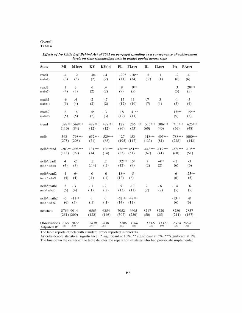
65

Overall Table 6

Effects of No Child Left Behind Act of 2001 on per-pupil spending as a consequence of achievement

levels on state standardized tests in grades pooled across state

State MI MI(w) KY KY(w) FL FL(w) IL IL(w) PA PA(w) read1 -4 2 .04 -.4 -20* -18** .5 1 -2 .4 (suba1) (3) (3) (2) (2) (11) (34) (.7) (1) (6) (6) read2 1 3 -1 .4 9 9** 3 20*** (suba2) (4) (3) (2) (2) (7) (5) (5) (5) math1 -6 .4 -2 -.7 15 13 -.7 .3 -1 -5 (subb1) (5) (4) (2) (2) (12) (10) (7) (1) (5) (4) math2 6 6 -4* -.3 18 41** 15*** 15*** (subb2) (5) (5) (2) (3) (12) (11) (5) (5) trend 397*** 569*** 488*** 478*** 128 206 *** 515*** 306*** 711*** 625*** (110) (84) (12) (12) (86) (53) (60) (40) (56) (48) nclb 368 798*** -652*** -529*** 127 153 618*** 405*** 788*** 1000*** (275) (208) (71) (68) (195) (117) (133) (81) (228) (143) nclb*trend -283** -298*** 131*** 106*** 456*** 451*** -448*** -119*** -271*** -105** (118) (92) (14) (14) (83) (51) (62) (41) (60) (51) nclb*read1 4 -2 .2 .2 32*** 15* .7 -4** -.2 -3 (nclb * suba1) (4) (3) (.14) (.2) (12) (9) (2) (2) (6) (6) nclb*read2 -1 -6* 0 0 -18** -5 -6 -25*** (nclb * suba2) (4) (4) (.1) (.1) (12) (6) (6) (5) nclb*math1 5 -.3 -.1 -.2 5 -17 .2 -.6 -.14 6 (nclb* subb1) (5) (4) (.1) (.2) (13) (11) (2) (2) (5) (5) nclb*math2 -5 -11** 0 0 -62*** -49*** -13** -8 (nclb * subb2) (6) (5) (.1) (.1) (14) (11) (6) (6) constant 8766 9014 6563 6354 7052 6605 8217 8720 8280 7857 (251) (209) (122) (146) (307) (230) (50) (35) (211) (167) Observations 7079 7072 2830 2830 1206 1206 11321 11321 8978 8978 Adjusted R2 .407 .570 .744 .784 .666 .825 .589 .690 .630 .721

The table reports effects with standard errors reported in brackets. Asteriks denote statistical significance: * significant at 10%, ** significant at 5%, ***significant at 1%. The line down the center of the table denotes the separation of states who had previously implemented

66

Table 7

Effects of No Child Left Behind Act of 2001 on percent differences in per-pupil spending, controlling for performance levels on state standards tests

Grade MI M I(w) KY KY(w) FL FL(w) IL IL(w) PA PA(w)

trend 5%*** 6%*** 6%*** 6%*** 1%* 2%*** 5%*** 3%*** 7%*** 6%*** nclb 5%** 7%*** -7%*** -4%*** 2% 2%* 6%*** 4%*** 9%*** 10%*** nclb*trend -3%*** -3%*** 1%*** 1%*** 5%*** 5%*** -4%*** -1%*** -3%*** -1%**

Asteriks denote statistical significance: * significant at 10%, ** significant at 5%, ***significant at 1%. The line down the center of the table denotes the separation of states who had previously implemented school finance reforms (left side) as compared to those who had not. Estimates are rounded to whole numbers where possible.

References

1. Adams, Jacob E, Jr. 1994. Spending Reform Dollars in Kentucky: Familiar Patterns and New Programs, but Is This Reform?. Education Evaluation and Policy Analysis, 16, No. 4 (Winter), http://www.jstor.org/stable/1164364.

2. Adams, Jacob E, Jr. 1997. School Finance Policy and Students’ Opportunities to Learn: Kentucky’s Experience. The Future of Children, 7, No. 3 (Winter), http://www.jstor.org/stable/1602447.

3. Adams, Jacob E, Jr. and William E. White II. 1997. The Equity Consequence of School Finance Reform in Kentucky. Education Evaluation and Policy Analysis, 19, No. 2 (Summer), http://www.jstor.org/stable/1164208.

4. Augenblick, John G., John L. Myers and Amy Berk Anderson. 1997. The Future of Children, 7, No. 3, Financing Schools (Winter), http://www.jstor.org/stable/1602446.

5. Bauries, Scott R. 2006. Florida’s Past and Future Roles in Education Finance Reform Litigation. Journal of Education Finance, 32, No. 1 (Summer).

6. Borman, Kathryn M., Tamela McNulty Eitle, Deanna Michael, David J. Eitle, Reginald Lee, Larry Johnson, Deirdre Cobb-Roberts, Sherman Dorn and Barbara Shircliffe. 2004. Accountability in a Postdesegregation Era: The Continuing Significance of Racial Segregation in Florida's Schools.American Educational Research Journal, 41, No. 3, Accountability and Equity (Autumn), http://www.jstor.orgstable/3699440.

7. Carmichael, Paul H. 1997. Who Receives Federal Title I Assistance? Examination of Program Funding by School Poverty Rate in New York State. Educational Evaluation and Policy Analysis, 19, No. 4 (Winter) http://www.jstor.org/stable/1164449.

8. Carnoy, Martin and Susanna Loeb. 2002. Does External Accountability Affect Student Outcomes? A Cross-State Analysis. Educational Evaluation and Policy Analysis, 24, No. 4 (Winter), http://www.jstor.org/stable/3594120.

67

9. Dee, Thomas S. 2000. The Capitalization of Education Finance Reforms. Journal of Law and Economics, 43, No. 1 (April), http://www.jstor.org/stable/725751.

10.Ehrenberg, Ronald G. Ehrenberg, Randy A. Ehrenberg, Christopher L. Smith, and Liang Zhang. 2004. Why do School District Budget Referenda Fail?. Educational Evaluation and Policy Analysis. 26, No. 2 (Summer). http://www.jstor.org/stable/3699555.

11.Fernández, Raquel, and Richard Rogerson. 1998. Public Education and Income Distribution: A Dynamic Quantitative Evaluation of Education-Finance Reform. The American Economic Review 88, No. 4, (September), http://www.jstor.org/stable/117007.

12.Greenwald, Rob, Larry V. Hedges and Richard D. Laine. 1994. An Exchange: Part I: Does Money Matter? A Meta-Analysis of Studies of the Effects of Differential School Inputs on Student Outcomes. Educational Researcher. 23, No. 3 (April), http://www.jstor.org/stable/1177220.

13.Greenwald, Rob, Larry V. Hedges and Richard D. Laine. 1996. The Effect of School Resources on Student Achievement. The Review of Education Research 66, No. 3 (Autumn), http://www.jstor.org/stable/1170528.

14.Guthrie, James W. 1974. School Finance Reform: Acceptable Remedies for Serrano. The School Review, 82, No. 2, Law and Justice in Education (February), http://www.jstor.org/stable/1084109.

15.Hanushek, Eric. 1971. Teacher Characteristics and Gains in Student Achievement: Estimation Using Micro Data. The American Economic Review, 61, No. 2. Paper presented at the Eighty-Third Annual Meeting of the American Economic Association, May, 1971 in New Orleans, USA. http://www.jstor.org/stable/1817003.

16.Hanushek, Eric. 1986. The Economics of Schooling: Production and Efficiency in Public Schools. Journal of Economic Literature, 24, No. 3 (September), http://www.jstor.org/stable/2725865.

17.Hanushek, Eric A. 1996. A More Complete Picture of School Resource Policies. Review of Educational Research, 66, No. 3 (Autumn), http://www.jstor.org/stable/1170529.

68

18.Hess, Frederick M. and Chester E. Finn Jr., eds. 2007. No Remedy Left Behind: Lessons from a Half-Decade of NCLB. Washington: The AEI Press. http://www.aei.org/books/bookID.902/book_detail.asp.

19.Hoxby, Caroline M.. 2001. All School Finance Equalizations Are Not Created Equal. The Quarterly Journal of Economics, 116, No. 4 (November). http://www.jstor.org/stable/2696457.

20.Hoxby, Caroline M. 1996. Are Efficiency and Equity in School Finance Substitutes or Complements?. The Journal of Economic Perspectives, 10, No. 4 (Autumn), http://www.jstor.org/stable/2138554.

21.Howell, Penny L. and Barbara B. Miller. 1997. Sources of Funding for Schools. The Future of Children, 7, No. 3, Financing Schools (Winter), http://www.jstor.org/stable/1602444.

22.Kim, James S., and Gail L. Sunderman. 2005. Measuring Academic Proficiency Under the No Child Left Behind Act: Implications for Educational Equity. Educational Researcher, 34, No. 8 (November).

23.Lee, Jaekyung and Kenneth K. Wong. 2004. The Impact of Accountability on Racial and Socioeconomic Equity: Considering Both School Resources and Achievement Outcomes. American Educational Research Journal, 41, No. 4 (Winter), http://www.jstor.org/stable/3699464.

24.LeFevre, Andrew T., Report Card on American Education: A State-by-State Analysis, 1985-1986 to 2006-2007 , Matt Warner, Editor. The American Legislative Exchange Council, 2008. Washington, DC

25.Linn, Robert L., Eva L. Baker, and Damian W. Betebenner. 2002. Accountability Systems: Implications of Requirements of the No Child Left Behind Act of 2001. Educational Researcher, 31. No. 6 (August-September), https://www.aera.net/uploadedFiles/Journals_and_Publications/Journals/Educational_Researcher/3106/3106_Linn.pdf.

26.Ludwig, Jens, and Laurie J. Bassi. 1999. The Puzzling Case of School Resources and Student Achievement. Educational Evaluation and Policy Analysis, 21, No. 4 (Winter), http://www.jstor.org/stable/1164484.

27.Manna, Paul, 2007. “NCLB in the States: Fragmented Governance, Uneven Implementation” in No Remedy Left Behind: Lessons from a Half-

69

Decade of NCLB, ed. Hess, Frederick M. and Chester E. Finn Jr., 15-42. Washington: The AEI Press. http://www.aei.org/books/bookID.902/book_detail.asp

28.Manwaring, Robert L. and Steven M. Sheffrin. 1997. Litigation, School Finance Reform, and Aggregate Educational Spending. International Tax and Public Finance, 4, No. 2, (March).

29.McCarthy, Martha M.. 1994, The Courts and School Finance Reform. Theory into Practice, 33, No. 2, Financing Education (Spring), http://www.jstor.org/stable/1476568.

30.Moser, Michele and Ross Rubenstein. 2002. The Equality of Public School District Funding in the United States: A National Status Report. Public Administration Review, 62, No. 1 (January-February), http://www.jstor.org/stable/3110283.

31.Murray, Sheila, William N. Evans and Robert M. Schwab. 1998. Education-Finance Reform and the Distribution of Education Resources. The American Economic Review, 21, No. 3, 88, (September), http://www.jstor.org/stable/117006.

32.Odden, Allen. Decentralized Management and School Finance. 1994. Theory into Practice, 33, No. 2, “Financing Education” (Spring), http://www.jstor.org/stable/1476570.

33.Odden, Allan and William H. Clune. 1998. School Finance Systems: Aging Structures in Need of Renovation. Educational Evaluation and Policy Analysis, 20, No. 3 (Autumn), http://www.jstor.org/stable/1164490.

34.Paris, Michael. 2001. Legal Mobilization and the Politics of Reform: Lessons from School Finance Litigation in Kentucky, 1984-1995. Law and Social Inquiry, 26, No. 3 (July), http://www.jstor.org/stable/829113.

35.Powers, Jeanne M. 2004. High-Stakes Accountability and Equity: Using Evidence from California's Public Schools Accountability Act to Address the Issues in "Williams v. State of California". American Educational Research Journal, 41, No. 4 (Winter, 2004), http://www.jstor.org/stable/3699463.

70

36.Roy, Joydeep. 2003. Impact of School Finance Reform on Resource Equalization and Academic Performance: Evidence from Michigan. Education Research Section. Working Paper No. 8., Princeton University http://repec.org/esNASM04/up.29436.1075499849.pdf.

37.Silva, Fabio and Jon Sonstelie, 1995. Did Serrano Cause a Decline in School Spending? National Tax Journal, 48, Issue 2 (June ).

38.Smith, Kevin B. 1994. Policy, Markets, and Bureaucracy: Reexamining School Choice. The Journal of Politics, 56, No. 2 (May), http://www.jstor.org/stable/2132149.

39.U.S. Department of Education, Office of Planning, Evaluation and Policy Development, Policy and Program Studies Service, State Education Indicators With a Focus on Title I, 2002-03, Washington, D.C., 2007

40.Walber, Herbert J., and William J. Fowler, Jr. 1987. Expenditure and Size Efficiencies of Public School Districts. American Educational Research Association, 16, No. 7 (October), http://www.jstor.org/stable/1174684.

41.Wilkins Rickman, Linda. 1981. School Finance Reform Litigation: A Historical Review. Peabody Journal of Education, 58, No. 4, Issues and Trends in American Education (July), http://www.jstor.org/stable/1491838.

42.Wilson, Lois and Joan Gavrilik. 1989. Education Aid in New York State: Targeting Issues and Measures. Publius, 19, No. 2, “Targeting by the States: The Basic Issues” (Spring, 1989), http://www.jstor.org/stable/3330442.

43.Wong, Kenneth K. 1991. State Reform in Education Finance: Territorial and Social Strategies. Publius 21, No. 3, “The State of American Federalism” (Summer), http://www.jstor.org/stable/3330518.

71