education and freedom of choice: evidence from arranged...

Education and Freedom of Choice: Evidence from Arranged

Marriages in Vietnam

M. Shahe Emran1

Fenohasina MaretStephen C. Smith

Department of EconomicsGeorge Washington University

This Version: November 2009

ABSTRACT

Using household data from Vietnam, we provide evidence on the causal effects of ed-ucation on freedom of spouse choice. We use war disruptions and spatial indicators ofschooling supply as instruments. The point estimates indicate that a year of additionalschooling reduces the probability of an arranged marriage by about 14 percentage pointsfor an individual with 8 years of schooling. We also estimate bounds that do not relyon the exact exclusion restrictions (lower bound is 6-7 percentage points). The impact ofeducation is strong for women, but much weaker for men.

JEL Classification Number: I2, O12, D1, J12Key Words: Arranged Marriage, Education, Schooling, Freedom of choice, Development,Vietnam, Social Interactions.

1We would like thank Robert Pollak, James Foster, Bryan Boulier, Justin May, Leonardo Magnusson,Chris Taber, Todd Elder, Forhad Shilpi, Shawn McHale, Tony Castleman, Zhaoyang Hou, and participantsat the AEA conference 2009 at San Francisco and Southern Economic Association Annual Conference 2009at Washington DC for helpful comments on an earlier version of the paper. The standard disclaimerapplies. Emails: [email protected]; [email protected]; [email protected].

1

(1) Introduction

There is a broad consensus among development practitioners, policy makers, and aca-

demic researchers that education is one of the most effective interventions to reduce poverty

and promote development. A large empirical literature on economics of education, in the

context of both developed and developing countries, focuses on the labor market returns to

education (Card (1995, 2001), Angrist and Krueger (1990, 1992), Duflo (2001), Alderman et

al (1996), Heckman (2005), Heckman and Li (2003), Glewwe (1996), among others). There

is a relatively small literature that focuses on the direct productivity effects of education,

especially in the context of self-employment in agriculture and non-farm activities (Jamison

and Lau (1982), Yang and An (2002), Kurosaki and Khan (2006)). A substantial litera-

ture in growth theory identifies human capital as a critical ingredient for long-run growth

(see, for example, Romer (1989,1994), Aghion et al (1998), Acemoglu (2009)), although

the empirical literature has been more mixed in identifying the effects of human capital in

cross-country growth regressions (Durlauf et. al. (2005)). A related literature addresses

whether social returns to education are significantly higher than the private returns due to

positive externalities (Acemoglu and Angrist (2000), Basu et al (2001)).

However, education confers many benefits to an individual (and the society) beyond the

returns in the labor market or its direct productivity and growth effects. As Amartya Sen

noted “[Education] can add to the value of production in the economy and also to the income

of the person who has been educated. But even with the same level of income, a person may

benefit from education in reading, communicating, arguing, in being able to choose in a

more informed way, in being taken more seriously by others and so on” (Sen (1999), p. 294).

The returns to education in non-market activities, especially as an input in the household

1

production function have been the focus of a significant strand of literature (Haveman and

Wolfe (1984, 2002), Kenkel (1991), Behrman and Wolfe (1987), Rosenzweig and Schultz

(1989)). The focus of this paper is on non-market returns to education beyond health and

productivity gains emphasized in the current literature; broadly, we are interested in returns

to education in social interactions. More specifically, we focus on the question of whether

education improves an individual’s freedom of choice by strengthening his/her bargaining

position in social interactions, within the household and in other social settings. We address

this question using freedom to choose ones own spouse, one of the most important decisions

in human life, as an indicator of freedom of choice.

The existing literature on intra-household bargaining focuses on the conflict of prefer-

ence between husband and wife, and analyzes its implications for control over resources

(Browning (1998), Lundberg and Pollak (1996), Haddad and Kanbur (1990)). In contrast,

our focus is on the bargaining between the parents and children under the assumption that

the preferences of parents with respect to the spouse choice is not fully aligned with the

preference of children. Since our interest lies in understanding the implications of educa-

tion for freedom of choice, we define arranged marriage as the cases where parents wield

the primary decision making power; they choose the spouse of children with or without

children’s input. Conversely, freedom of choice refers to the cases where children are the

primary decision makers; they choose their spouse with or without parental input.2

Parents in developing countries make decisions about the education of their children

when they are young, taking into account a multitude of factors including old-age support,

2The binary arranged marriage variable used in this paper, by definition, cannot capture finer shadesin the bargaining game between the parents and children. We, however, believe that our definition isa reasonable representation of the idea that arranged marriage indicates less freedom of choice for thechildren.

2

social status, and pure altruism. There is, however, a trade-off from the parents’ perspec-

tive: a more educated child may be more able to take care of them in old age and bring in

social prestige, but he/she is also likely to exert more bargaining power in decision making

(because of better outside options derived from improved economic opportunities and social

networks). The bargaining game between children and parents thus changes significantly

after education is acquired. This implies that, ceteris paribus, better educated children

would be more likely to choose their own spouse. We use household survey data from

Vietnam in 1995 (from Vietnam Longitudinal Survey (VLS), 1995-98) to examine whether

better education among children reduces the incidence of arranged marriage.

To the best of our knowledge, there is no empirical analysis of the causal effects of edu-

cation on the arranged marriage in economics literature. There is a sociological literature

that uses rich case study methods and multivariate statistical models to investigate the

relationship between arranged marriage and education of children (e.g. Jejeebhoy, 1995).

In general, they however do not disentangle the causality issue. This paper is thus the first

attempt in the literature to estimate the causal effects of education on arranged marriage.

Identification of the causal effects of education on choice of spouse can be challeng-

ing. Addressing omitted variables bias due to unobserved individual ability as well as

unobserved individual and parental preferences is important in estimating the effects of

education on spouse choice. Any observed negative partial correlation between the proba-

bility of arranged marriage and the level of education might be driven by such unobserved

heterogeneity that affects both schooling attainment and spouse choice decisions. For ex-

ample, more “progressive” parents are more likely to invest in the education of children

and also find it acceptable to allow the children to choose their own spouse. A stubborn

3

child might be more successful in withstanding the pressure to drop out of school for early

marriage, and thus may have higher education. He/she is also likely to be more emphatic

in defending his/her own choice of spouse. It is, however, also possible that a stubborn

child drops out of school as a rebellion to parental preference for education, and also does

not allow the parents to choose the spouse for him/her. Such unobserved heterogeneity

would lead to a biased estimate of the effects of children’s education on spouse choice in

an OLS regression. Note also that it is not possible to pin down the direction of such bias

from a priori reasoning.

The household survey from Vietnam used in this paper is especially suitable for isolating

the effects of education for a number of reasons. There is good information on individual

and parental characteristics and labor market opportunities. Also, the data come from 10

communes located in the Red River Delta region in Vietnam, and thus exhibit little or no

variations in cultural practices. This implies that cultural heterogeneity is not likely to

drive the results we report in this paper.3 The empirical results provide robust evidence

in favor of a statistically significant and numerically important negative effect of education

on the probability of arranged marriage.4

The presence of multi-level unobserved characteristics makes it much harder to find

suitable instrumental variables, especially to defend the exclusion restrictions.5 Note that

3The Red River Delta is the center of ethnic Vietnamese culture. Vietnamese families are usuallycharacterized as part of a Confucian patrilineal, patrilocal, and patriarchal cultural heritage (Keyes, 1996).

4The incidence of arranged marriage in the sample used for estimation is 25 percent. The surveywas carried out by a group of Vietnamese and American sociologists in 1995, and a large number ofrespondents (63 percent) belong to birth cohorts before 1960. The incidence of arranged marriage is likelyto have declined significantly in recent years in Vietnam because of expansion of education and improvedlabor market opportunities, among other things. In fact, the results presented in this paper imply that theprobability of arranged marriage should become very small once an individual in Vietnam attains 10 yearsof schooling.

5The randomized assignment of one year of additional schooling is not possible, a point emphasized byAngrist and Krueger (2001). Thus one has to rely on other sources of potential exogeneous variations in

4

the exclusion restrictions imposed in an IV framework are exact, i.e., the coefficient of

the excluded instruments are assumed to have exactly zero coefficients in the structural

equation (in our case, the equation for arranged marriage). This sharp exclusion restriction

needed for the validity of the IV approach has led to increasing skepticism in the literature.

As pointed out recently by Conley et al. (2008) it may be more credible to assume that the

instruments satisfy the exclusion restrictions approximately, i.e., the instruments may have

non-zero but very small effects in the structural equation. In addition to the standard IV

results, we thus report estimates from the bounds approach developed by Conley et. al.

(2008) under the assumption that the instruments satisfy the exclusion restrictions only

approximately.

We follow a large and mature literature on returns to education and use indicators

of supply of schooling and exogenous shocks to schooling attainment as instruments (see,

Card (2001), Blundell et. al. (2005)). More specifically, we use birthplace and a binary

cohort dummy for birth year 1955 and earlier as identifying instruments in this paper.6

Birthplace represents variations in schooling supply across geographic locations, while the

1955 cohort dummy captures positive shocks to educational attainment of 1955 and earlier

cohorts due to lower intensity of conflicts in North Vietnam over 1954-1965 (see below).

Birthplace is a good indicator of access to schools only if someone grows up in the same

place. In our data set, 98.7 percent of individuals grew up in the place of birth.7

The cohort dummy represents differences in schooling attainment of the cohort born

years of schooling for identification.6The birthplace and cohort dummies have been used as instruments for education for example by Schultz

(2002), among others.7There are 27 birthplace dummies we can use as instruments. With only one endogeneous regressor, this

is likely to create a weak IV problem due to too many instruments. As a result, we reduce the dimensionof the the instruments sets in the empirical implementation. For details, please see P.17 below.

5

after 1955 compared to the older cohort (above 40 years of age in 1995). In our sample

43 percent of individuals are born before 1955. A plausible interpretation of this dummy

variable is that it captures the effects of varying intensity of conflicts and war experienced

by different age cohorts when they were school aged. The history of war and conflict in

Vietnam is long and complex; the intensity of conflict varied over time and space signifi-

cantly. The cohorts born before 1955 in the Red River Delta region experienced a relatively

stable period from 1954 to 1965 which is expected to improve their educational attainment

compared to the later cohorts.8 For the Red River Delta region, the disruptions caused by

US bombing in the late sixties to mid seventies were severe and the later cohorts are likely

to suffer negative shocks to their educational attainment.9 Especially, the 10 communes

surveyed for our data set were bombed heavily because of their proximity to important rail

road links and industrial installations (Merli, 2000, P. 4). The education of the later co-

horts were affected adversely also because of mass mobilization for the American war. The

empirical results reported later show that the earlier cohorts did experience systematically

higher educational attainment after controlling for a vector of individual and household

level variables and the rural-urban dummy.10 One might worry that intensity of conflict

can have direct effect on marriage market because it affects the sex ratio. The changing

sex ratio may also affect the incentives for human capital investment by parents if such

8For discussions on wars in Vietnam, see Harrison, 1989; Young, 1991.9The US aerial bombing of North Vietnam started on March 2 1965 with Operation Rolling Thunder.

Another major air campaign was waged in December 1972 which came to be known as Operation LinebackerII.

10One can argue that the oldest age cohort, born long before 1954, would not experience the fruits ofrelative calm during the 1954-65 period, as they would have been past their school age. Thus one shouldfocus on an interval of age cohort excluding the oldest age cohorts. As part of robustness checks, we excludethe too old cohorts and define a dummy for year of birth between 1945-55. The main conclusion of thispaper is not sensitive to this alternative definition of the cohort dummy and we omit the results for sakeof brevity.

6

investments respond to potential returns in the marriage market (LaFortune, 2009). We

thus include age cohort specific sex ratio as an additional control in the regressions (cal-

culated using the 1979 census in Vietnam).11 Another potential objection to the exclusion

restriction imposed on the cohort dummy is that it might proxy for changing formal rules

or informal norms regarding marriage. We control for age of the respondent to account

for changing views regarding arranged marriage across different generations. In addition,

a dummy for marriages before 1960 is included to account for reform of marital law in

Vietnam enacted in 1960.

For birthplace to qualify as a reasonable instrument in our context, we need to control

for differences in the labor market opportunities. Such opportunities are likely to vary

across geographic locations, and are important determinants of both the incidence of ar-

ranged marriage (Goode (1963)) and investment in human capital.12 Better labor market

opportunities improve children’s outside option if they have to leave their parental house

and are deprived from parental wealth as a consequence of choosing their own spouse. We

include an indicator of non-agricultural occupational opportunities at the time of marriage,

a rural urban dummy, and household’s wage income to control for local labor market op-

portunities.13 The rural-urban dummy also captures differences in living costs, especially

housing costs. As mentioned before, in addition we control for a number of individual, and

11Observe that the changing sex ratio primarily affects the bargaining between the bride and bridegroom.Since war is likely to negatively affect the availability of eligible men in the marriage market, it would tendto improve the bargaining position of men (and their parents) vis a vis the women (and their parents).However, there are no compelling reasons to believe that it would affect the bargaining between the parentsand children which is the focus of this paper.

12For an analysis of role of labor market opportunities for transition from arranged marriage to freespouse choice in medieval Europe, see de Moor and Van Zanden (2005).

13Since most of agriculture consists of self employment, the non-farm occupation is a reasonable indicatorof labor market opportunities. If we use finer occupational categories at the time marriage instead, themain results of the paper remain robust.

7

parental characteristics that help isolate the causal effects of education on spouse choice.

The evidence from the formal test of exogeneity discussed below (see section 4.1 and

Table 3) show that conditional on the set of control variables, the birthplace and age cohort

dummy satisfy the exclusion restrictions unambiguously (P-value of Hansen’s J statistic is

0.81).14

The empirical results indicate that education does significantly reduce the likelihood

of having an arranged marriage. Averaging the point estimates from linear probability

(2SLS, GMM, CUE-GMM) and Probit (Control Function and IV Probit) models imply

that one year of additional schooling reduces the probability of arranged marriage by about

14 percentage points for an individual with 8 years of education. The probability that an

individual will have an arranged marriage is close to zero when he/she has about ten years of

schooling. The results from bounds analysis using the Conley et al (2008) approach provide

strong evidence of a negative causal effect of education on the probability of arranged

marriage; none of the bounds contain zero. The lower bound estimates indicate a smaller

effect of education; one year of additional schooling reduces the probability of arranged

marriage by about 6-7 percentage points for an individual with 8 years of education. The

results from the bounds analysis are important as they show that the central conclusion

in this paper does not depend on the exclusion restrictions imposed in the IV approach.

The results also suggest that the effects of education has important gender dimension. The

impact of education is very strong for women; the marginal effect is about 17 percentage

points for a woman with the average level of education (7.77 years of schooling). The

evidence in favor of a significant causal effect of education on arranged marriage in case

14For more complete discussion of the identification issues and the roles played by different controlvariables, please see section 4 below.

8

of men is, however, much weaker. To the best of our knowledge, this is the first paper in

the literature to provide evidence on the causal effects of education on freedom of spouse

choice.

We organize the remainder of the paper as follows. The first section discusses the

conceptual framework which helps us identify the relevant control variables. The next

section provides a brief discussion of the data source and variables descriptions. Section 4,

arranged in subsections, is devoted to the empirical strategy used in this paper to identify

and estimate the causal effects of education on freedom of spouse choice. Section 5 presents

estimates of causal effects of education on arranged marriage using an instrumental variables

approach and the bounds approach due to Conley et al (2008). In the conclusions, we

provide a summary and context of the results and contributions of the paper.

(2) Conceptual Framework

Arranged marriage is common in many developing countries, especially in Asia and

Africa. There are reasons to believe that in many cases it is not a cooperative outcome

where parents and children jointly choose a spouse to maximize family welfare.15 There

are no a priori reasons to expect that the preferences of parents and children would be

perfectly aligned.16 Parents might be interested in arranged marriage to further their

15To the best of our knowledge there is no evidence on the suitability of a unitary model to explainintrahousehold decisions between parents and children. There is, however, overwhelming evidence againstthe unitary model in the context of intrahousehold allocations between husband and wife (see, for example,Haddad and Kanbur (1990), Lundberg and Pollak (1996)).

16We would also note that even in the cases of apparent general agreement, there is plenty of room forspecific disagreement. Even if the principle of arranged marriage is agreed, in most cases there are likelyto be several potential partners, and the parents and children may rank order them differently. It is notpossible to analyze this type of conflict of preference within the arranged marriage with our data.

9

objectives of strengthening their own social and business network, to improve their standing

in the community, and to uphold cultural traditions. Another important motive is old-age

support; if the parents choose the spouse it is less likely that the spouse of their children will

skew the distribution of resources against them, especially in old age. It has been argued

that the transition from arranged marriage to own choice redistributes resources away from

the parents to the children, and it might have implications for savings and growth (Edlund

and Lagerlof (2006)).

The practice of arranged marriage seems to decline generally with economic develop-

ment; the expansion of education and labor market opportunities for children are negatively

correlated with the incidence of arranged marriage (for a discussion, see Goode (1963)).

There is a substantial literature in sociology that provides suggestive evidence of a negative

correlation between education and the probability of having arranged marriage in a society

(for a summary, see Jejeebhoy (1995)). Education can influence the spouse choice through

a variety of channels. It may mould children’s preference, enrich the pool of potential

partners, and alter the threat point in the bargaining game in favor of children. The

changes in preference can be due to interactions with people with different attitudes to

arranged marriage, exposure to other cultural norms, and in general through a broadening

of outlook. Social interactions at the school and college may increase the pool of potential

partners with similar values and thus of better compatibility. Education alters the threat

point in the bargaining game between parents and children, because educated children in

general have better outside options (labor market prospects and higher permanent income).

In the event of a conflict regarding spouse choice, the parents can use a prospective be-

quest as a threat, i.e., they might redistribute away from a son or daughter who choose

10

his/her own spouse. They can also threaten to drive the newly married couple from the

parental home, an effective deterrent when the housing and other related costs of starting a

separate household is high enough.17 Educated children are also more equipped to handle

the pressure from parents which sometimes may take the form of legal and other forms of

harassment when they choose their own spouse. Finally, extended schooling tends to delay

the age at marriage, thereby placing the spouse choice decision at a time when the children

are more mature and capable of making better choices.

As mentioned before, the fact that education may weaken parent’s influence on chil-

dren in general, and on spouse choice in particular, also implies that parents will take into

account this additional cost when making the education decisions for their children. This

has interesting implications for allocation of resources across different children for educa-

tion. Parents might trade off potentially higher earnings for more compliant behavior of

children, assuming that the correlation between ability and assertiveness is positive. This

is likely to result in a negative selection effect in our context because parents would invest

more in educating the more pliant children even though they may be of lower ability, and

the more pliant a child is, the easier it is for parents to overrule his/her spouse choice.

A related issue which might create a spurious negative correlation between education and

arranged marriage is the possibility that the parents arrange marriage while the child is

attending school, and his/her education is truncated as a result of the marriage. This,

however, seems not to be a problem in our data set, as there are only a few observations (21

observations out of 4464) where the timing of marriage corresponds to that of withdrawal

from school.

17For a theoretical analysis of arranged marriage where fixed costs of new household formation plays animportant role, see Dasgupta et al (2008).

11

(3) Data

We use data from the Vietnam Longitudinal Survey (VLS, 1995-98) conducted by re-

searchers from the University of Washington and Institute of Sociology in Hanoi18. The

choice of this data set is motivated by the fact that that it has information on choice of

spouse in addition to information on individual and parental characteristics, and on labor

market opportunities. The data set is composed of 1185 households and covers 4464 indi-

viduals. It is a 4 year panel data set. It would have been econometrically advantageous to

exploit the panel data, but for our variables of interest, in particular regarding the marital

status, there is no significant changes across various years. For example, only 42 among the

4464 have changed marital status during those 4 years. The empirical analysis of this paper

is based on the 1995 data. Because of missing observations for various variables (such as

years of schooling, age at marriage, number of parental siblings), our analysis is based on

a sample of 3219 observations.

The survey covers areas around the Red River Delta where there are a total of 10

communes partitioned into four groups: urban communes (3), within 3km of highway or

inter-provincial highway (2) and within 3-10km (2) and more distant than 10 km (3).

About 80% of the 4,464 individuals interviewed were married. The characteristics of the

sample used for estimation (3219 observations) are reported in Table 1. For our variable

of interest ‘arranged marriage’, the parents chose the spouse with or without consultation

with children for 25% of married individuals. Interestingly, there is no evidence of gender

differences in the incidence of arranged marriages. The average age in the survey year

(1995) is 39 years, with 63 percent of the sample born before 1960. The average education

18http://csde.washington.edu/research/projects/hirschman/vietnam/vls.html

12

is about 8.07 years of schooling, and 82 percent of individuals had more than 5 years of

schooling. The educational attainment for men is higher; the average education in the

sample of men is 8.58 years of schooling, while the average for women is 7.77 years. The

education system in Vietnam is standard in that students graduate from high-school after

12 years of schooling. We recoded the years of schooling variable by assigning 13.5 years

of education if the person has attended college but did not finish, and 15 if the person has

attended and finished college. The average age at marriage is 22.54 years which indicates

that early marriage may not be that common (6.5 percent below 18 years). Only 4 percent

of individuals met their spouse at school. This implies that schools do not play an important

role as a meeting place for potential marriage partners.

(4) Empirical Strategy

To test the hypothesis that education has a causal effect on the incidence of arranged

marriage, we estimate the following Probit model:19

P (Yi = 1|Xi) = Φ(β0 + β1Ei + X

′iΠ + εi

)(1)

Yi is a binary variable that takes on the value of 1 if the marriage was decided by the

parents for individual i and 0 if he/she chose his/her own spouse with or without parent

approval and Φ(.) is the standard normal CDF. The level of educational attainment by

individual i is represented by Ei, and Xi is a vector of relevant control variables. The

error term in equation (1) captures unobserved heterogeneity of both parents and individ-

19In the empirical implementation, we also report results from linear probability model which do notdepend on distributional assumption.

13

ual i. Educational attainment is measured by ‘years of schooling’. The vector of control

variables include a rich set of household and individual level characteristics. As mentioned

before, an advantage of the data set used in this paper is that it has good information

on characteristics of an individual, his/her parents (both mother and father) and also on

labor market opportunities.20 The parental characteristics include occupation, birth order

(if first born), and number of sibling. Occupation is a choice variable of the parents and

thus would reflect their preference and ability. The number of siblings and birth order of

a child might plausibly affect the the nature of the bargaining game between parents and

children. We also include indicators of fertility choices of both parents and grand parents

(the numbers of own and parents’ siblings). A smaller family size may be an indicator of

more “progressive” views in general.21 Individual level variables for children include age,

gender, age at marriage, a dummy for no religious affiliation, and number of siblings. It

is important to control for the gender of the child as parents may have son preference.

The age at marriage may influence the nature of bargaining between parents and children.

Religious affiliation is likely to influence ones views about acceptability of parental choice.22

We also control for a set of household level variables that might affect investment in

human capital and may also influence preference regarding arranged marriage (i.e., both ed-

ucation and freedom of choice may be normal good). Higher income households are, ceteris

20The data set also has information on the characteristics of the spouse. The characteristics of spousecan potentially be proxy variables for unobserved preference of parents and children. In the context ofarranged marriages, the characteristics of spouse might capture parental unobserved heterogeneity, as theyreflect parental preference. In case of own choice of spouse, they might reveal the preference of children.However, the characteristics of spouse are not exogeneous as they depend on the nature of spouse choice.We thus chose not to use them as controls. We, however, note that the estimates of the causal effect ofeducation on arranged marriage presented in this paper remain virtually identical if we include the spousalcharacteristics.

21We thank James Foster for suggesting this interpretation.22The sample consists of 17 percent Christian and 20 percent Buddhist, and 63 percent with no religion.

14

paribus, more likely to invest in children’s education because of relaxed credit constraint.

We use household’s agricultural and wage income as controls for income. In addition, a

dummy for brick-wall house and dummies for ownership of radio and TV are also included.

These are indicators for household wealth, and ownership of TV and radio also controls

for access to information which might affect views regarding acceptability of arranged mar-

riage. As we discuss in the following, children’s own age, wage income and the rural-urban

dummy play a critical role in our identification strategy.

As discussed before education may affect the probability of arranged marriage through

a number of channels including changes in the bargaining game and also better search and

information regarding the pool of partners in school. To isolate better the role played by

bargaining, we need to control for the fact that at least part of the effect of education would

capture the information and matching effect. We control for this information and matching

channel by including a dummy for the case when a person met his/her spouse at school.

(4.1) Approaches to Identification

Identification of the causal effects of education on probability of arranged marriage is

difficult due to multi-level unobserved heterogeneity in ability and preference. We use

an instrumental variables strategy and the recent bounds approach under the assumption

that instruments are ‘plausibly exogeneous’ to provide evidence on the causal effects of

education on arranged marriage.

Instrumental Variables Approach

Following a large literature on returns to education in the labor market, we use indi-

cators of schooling supply and shocks due to war as instruments for children’s education.

15

More specifically, the instruments used in this paper are birthplace and a dummy for birth

cohort above 40 years of age (born in or before 1955). The birthplace represents variations

in the supply of schooling across geographic locations, while the cohort dummy represents

variations over time due to varying intensity of conflict. The birthplace is a good indicator

of schooling supply only if the respondent grew up in the place of birth. In our data set, 98.7

percent of the respondents grew up in their place of birth. Labor market opportunities and

housing costs have been identified in the sociological literature as important determinants

of arranged marriage (Goode (1963)). We use an indicator of non-farm opportunities at

the time of marriage, wage income and a rural-urban dummy to capture the labor market

opportunities and housing market conditions. Controlling for labor market opportunities

is important for consistent estimation of the causal effects of education, because both edu-

cation and outside options of a child in the bargaining game depend on it. Better market

opportunities might induce the parents to invest more in children and also allow the chil-

dren to assert their preferences ex post by improving their outside option. The rural-urban

dummy also controls for differences in exposure to cultural factors (modernization).

One might argue that the birthplace of children is the location chosen by parents (es-

pecially by father in a patriarchal and patrilocal society like Vietnam), and some fathers

might choose location close to the school if they value education more. If the fathers who

value education more also differ systematically from other parents in their attitude to ar-

ranged marriage (for example, they may be more “progressive”), then this will weaken the

case for the exclusion restriction. However, there are good reasons to believe that, in the

specific context of our data set, this is not a concern. First, in our sample, the house-

hold location seems static and historically determined for most of the parental generation;

16

about 70 percent of fathers were born in the same place as the children. For the other 30

percent of cases, the birthplace of children reflects parental choice. However, unlike many

developed countries, the location choice in Vietnam is primarily determined by parental

occupation and labor market opportunities, and children’s school choice usually plays a

minor role. In the regressions, we thus control for parental occupation (both father’s and

mother’s occupation).23 The evidence presented below shows that conditional on the set

of observed covariates, the instruments comfortably satisfy the formal test of exogeneity

(P-value for Hansen’s J statistics is 0.81).

There are 27 birthplace dummies we can use as instruments along with the cohort

dummy. This, however, is likely to create weak IV problems due to too many instruments,

as we have only one endogeneous regressor. We thus need to reduce the dimension of the

instruments. Although the respondents in the survey were born in 27 different birthplaces,

most of the sample is concentrated in a few places. We define two dummies, one for the

case when the respondent was born in the same commune he/she is currently located in,

and the second one for the cases where respondent was not born in the current commune,

and the birthplace is the location with largest number of respondents among all the ‘other’

birthplaces. These two dummies represent 86 percent of the sample. The other 25 birth-

places together represent the excluded category. We also use an alternative approach where

the first two principal components (based on Eigen values) of the 27 birthplace dummies

represent the schooling supply variations across space. As noted early on by Amemia (1966)

and emphasized more recently by Bai and Ng (2008), using principal components to reduce

the dimension of the set of instruments work well in such cases. The results using this

23The lack of spatial mobility in Vietnam was reinforced, especially in the rural areas, by an identitycard system known as ho khau (residence registration book). The ho khau system was initiated in 1960.

17

alternative set of instruments are consistent with the conclusions reported in this paper.

For the sake of brevity, we do not report these alternative results.24

The cohort dummy (that equals 1 if born in or before 1955) reflects the difference in

schooling attainment between the cohorts born in 1955 and earlier and those born after

1955. Although Vietnam suffered a series of wars and conflicts, there was a relative calm

in North Vietnam from 1954 to 1965 (Harrison, 1989, Young, 1991, Merli, 2000). The age

cohorts born in 1955 and earlier, and in school during this period experienced a positive

shock to their schooling attainment. The later cohorts (born after 1955) experienced a

negative shock to education attainment which can be attributed, among other things, to

intensified US bombings in the Red River Delta region during Vietnam war and related

disruptions such as mass mobilization. As mentioned before, the communes that consist

the survey area of VLS 1995 used in this paper were heavily bombed because of their

proximity to important rail links or industrial installations. Using the VLS panel data set,

Merli (2000) shows that the war mortality was much higher during the US bombings in the

Red River Delta region compared to earlier periods.

An alternative discussed earlier is to use a cohort dummy for birth year between 1945-55

to capture the positive shock to education due to the stability from 1954-65 in the Red

River Delta region. The results from this alternative formulation of the cohort dummy are

very similar to the ones based on the 1955 cohort dummy, and thus are omitted to save

space.

One might argue that the cohort dummy may also reflect changes in the informal social

norms or formal legal codes regarding acceptability of arranged marriage. If there are

24The results are available from the authors.

18

significant changes in social norms or formal legal codes over the relevant time period, it

would result in heterogeneity in the incidence of arranged marriage across different cohorts

of children. To account for slowly changing social norms, we include age and age squared

of children. Age controls for possible generational changes in the views regarding arranged

marriage. There was also significant change in the marital law in Vietnam; the practice

of arranged marriage (and dowry) was made illegal in 1960. Not surprisingly, however,

the formal law did not take hold on the ground for a long time (Van Bich, 1999).25 We

include a dummy for marriage before 1960 to capture possible impact of this change in

the formal legal code on incidence of arranged marriage. Another potential objection to

the exclusion restriction on the cohort dummy mentioned before is that the conflict might

affect the marriage market directly through its effects on the sex ratio. We thus include

cohort specific sex ratio as an additional control.

Set Identification: Bounds Under Approximate Exclusion Restrictions

The instrumental variables approach outlined above is attractive because it provides us

with point identification. However, as mentioned before, the IV approach relies on exact

exclusion restrictions on the instruments which some readers might find too restrictive.

We thus use the recent approach developed by Conley et al (2008) where the exclusion

restrictions on the instruments are relaxed, but point identification is not possible. In the

context of our model, the exact exclusion restrictions imposed in the IV approach implies

25According to one observer, “(I)n fact, the implementation of these laws has not been simple, and thesocial reality is often far cry from the ideals posited by the law-makers. A massive effort is needed tomodify peoples thinking and to establish in the minds and behavior of the masses the new ideas aboutmarriage and the family. This requires education, and the elimination of not only long-standing traditions,but also misconceptions, and even strong opposition. The question is how to educate people to renouncethe traditions of polygamy, child marriages, arranged marriages,” P.59, Van Bich, 1999.

19

that H0 : θ1 = θ2 = 0 in the following specification of the spouse choice function:

P (Yi = 1|Xi) = Φ(β0 + β1Ei + X

′iΠ + θ1Vi + θ2Dc + εi

)(2)

where Vi is birthplace, and Dc is a dummy for age cohort (40 years cut-off). It may

be more plausible to argue that these exclusion restrictions hold only approximately, i.e.,

H0 : θ1 = θ2 ' 0, especially in an application like ours where there are multiple sources

of unobserved heterogeneity, and the instruments might have very small direct effects on

arranged marriage if they are proxy variables for omitted heterogeneity. Under the approxi-

mate exclusion restrictions, the instruments are “plausibly exogeneous” in the terminology

of Conley et. al. (2008) who develop a set of approaches under this weaker exogeneity

condition, and show that one can estimate bounds on the causal effect of the endogeneous

variable.

We implement a simple and intuitive approach to modeling “plausible exogeneity” of

the instruments as developed in Conley et. al. (2008); it specifies a support of possible

values for θj ∈ [−δ, +δ] where δ > 0 can be arbitrarily small. Under this assumption, we

estimate the lower and upper bounds for the estimate of the parameter of interest β1. We

report results for a number of alternative values of δ.

(5) Empirical Results

Preliminary Results

Figure 1 shows the predicted probability of arranged marriage (dummy equals 1 if mar-

riage was arranged by parents with or without children’s inputs) against different years of

20

schooling from a simple Probit regression of arranged marriage on education without any

controls. There is a clear negative relationship between education and the probability of ar-

ranged marriage. As discussed before, this bivariate correlation-while interesting in its own

right-cannot inform us about the possible causal effect of education due to omitted variables

bias. Table 2 presents results from estimating equation (1) above using Probit for different

sets of control variables. The corresponding results from OLS estimation are very similar,

and are reported in the Table A.1 in the appendix. The first column reports estimates with

only individual level controls and then we progressively include parental characteristics,

household level variables, labor market opportunities at the time of marriage and a rural-

urban dummy. The estimates show a consistently negative and statistically significant

effect of education on the probability of arranged marriage.26 Although suggestive of a

statistically significant negative effect of education on the probability of arranged marriage,

these results may suffer from omitted variables bias because of unobserved heterogeneity

in ability and preference of both parents and children. Another source of possible bias is

measurement error in schooling which would result in estimates biased downward. It is

thus not possible to pin down the direction of the bias from a priori reasoning.

Estimates from the IV Approach

The estimated effects of education on the probability of arranged marriage from the IV

approach are reported in Table 3. For estimation, we use IV Probit and a control function

26The Probit (Table 2) and linear probability model (Table A.1 in appendix) estimates show that theParents’ number of siblings (both father and mother) exerts a robust positive effect on the probability ofarranged marriage, while own number of siblings is not significant. Also, wage income is a robust negativedeterminant of arranged marriage. The 1960 legal reform dummy is significant indicating that the changein the formal law had some impact on the incidence of arranged marriage. Access to information (TV andradio) seems to reduce the probability of arranged marriage.

21

approach for the Probit model (Blundell and Smith (1986), Rivers and Vuong (1988));

while for the linear probability model 2SLS and GMM are used. With a binary dependent

variable, control function with Probit may provide more efficient estimates compared to

2SLS and GMM that ignore the binary nature of the dependent variable. The linear

probability model, on the other hand, has the advantage that it does not require any

distributional assumption.

The IV diagnostics show that the instruments pass the test of exogeneity convincingly;

the P-value of Hansen’s J statistic is 0.81. The estimates from first stage show that the

instruments have reasonable power; the F statistic for exclusion of the instruments is 12.49

which is higher than the Bound et al (1995) rule of thumb of 10 for one endogeneous

regressor. In the first stage regression, the cohort dummy is significant at the 5 percent

level, and the birthplace dummies are significant at the 1 percent level. Consistent with

the discussion before, the estimated coefficient on the cohort dummy shows that the cohort

born after 1955 has significantly lower educational attainment.

The first column in Table 3 (Panel A) shows the estimated effect of education using

the control function approach and the second column presents the results from IV Probit

(estimates are marginal effects evaluated at the sample mean). The control function results

show that education is clearly endogenous in the arranged marriage equation, as the residual

from the first stage is significant at the 1 percent level. The estimated marginal effect of

education on arranged marriage is significant both statistically and numerically. According

to the control function estimate, one year of additional schooling reduces the probability of

arranged marriage by 17 percentage points for an individual with 8.07 years of education

(the average level of education in the sample). The estimated marginal effect from IV

22

Probit is somewhat smaller; one year of additional schooling reduces the probability of

arranged marriage by 13 percentage points. The third (2SLS) and fourth (GMM) columns

in Table 3 report the results from the linear probability model. The estimated marginal

effects from these alternative estimators are identical to that from the IV Probit. The

estimates are statistically significant at the 1 percent level. The IV estimates from Probit

and linear probability models thus provide robust evidence in favor of a strong negative

effect of education on the probability of arranged marriage.

Although the strength of the instruments is reasonable, One might still worry about

possible weak IV bias. To address any such concerns, we report results from two alternative

checks. First, we use CUE-GMM to estimate the linear probability model and compare

the estimates with those from 2SLS. As pointed out by Hansen et al (1996) and emphasized

recently by Stock and Watson (2008), if the instruments are weak, then the CUE-GMM

estimates perform better than 2SLS, and would differ significantly from the 2SLS estimates.

The results from CUE-GMM are reported in the last column of Table 3. The estimated

marginal effect of education is 13 percentage points, exactly equal to the common estimate

from IV Probit, 2SLS, and GMM. Second, we use the recently developed tests for weak IV

robust inference in binary choice models with heteroskedasticity developed by Magnusson

(2008), and Finlay and Magnusson (2009). Panel B in Table 3 reports the results from the

Finlay and Magnusson (2009) approach to weak IV robust inference for the linear probabil-

ity and the Probit models. Note that the Probit results are for the estimated coefficients,

not for the marginal effects. We report the results from the Conditional Likelihood Ratio

(CLR) and Anderson-Rubin test. According to the conditional likelihood ratio (CLR) and

Anderson-Rubin (A-R) tests, the null of no effect of education on arranged marriage is

23

rejected at the 1 percent level (P-value=0). The 95 percent confidence intervals for CLR

and Anderson-Rubin tests do not include zero. The lower bound estimate from the 95

percent confidence interval gives an estimated marginal effect of about 7 percentage points

reduction in the probability of arranged marriage (estimates from linear probability model).

Relaxing the Exact Exclusion Restrictions: Estimated Bounds

In this section, we report results from the recent bounds approach developed by Conley

et. al. (2008). As discussed before, the exact exclusion restrictions are relaxed and we

model ‘plausible exogeneity’ of the instruments by assuming that the coefficients on the

instruments in the arranged marriage equation belong to an interval, i.e., θk ∈ [−δ, +δ]

∀k with δ > 0. The estimated bounds are reported for 95 percent confidence intervals in

Table 4 with δ = 0.0001, 0.0005, 0.001, 0.005, 0.01. The reported results are from the 2SLS

estimator.

The results show that the estimated bounds do not vary significantly with the value

of δ. More importantly, none of the 95 percent confidence intervals contain zero. This

is strong evidence in favor of a robust negative effect of education on the probability of

arranged marriage. The negative causal effect identified earlier in Table 3 are thus robust

to relaxation of the exact exclusion restrictions imposed on the instruments for the IV

estimates. It is reassuring that even if we allow for non-zero but low-level direct influence

of the instruments on the probability of arranged marriage, the central conclusion that

education reduces probability of having an arranged marriage remains intact. Even if one

uses the most conservative estimate from the lower bound, one year of additional schooling

still reduces the probability of arranged marriage substantially, by 6-7 percentage points.27

27Note that δ = 0.01 implies that each of the instruments can affect the probability of arranged marriage

24

Gender, Education and Arranged Marriage

The results discussed so far do not consider possible gender differences in the effects of

education on probability of arranged marriage. The results reported in Table 2 from Probit

model show that the gender of the respondent matters for arranged marriage. The results

reported in Table 2, however, cannot answer the question whether the effects of education

on arranged marriage are significantly different for a female compared to a male. In this

section we explore the issue of gender differences in the effects of education. Table 5 reports

the results from estimating equation (1) separately for male and female sub-samples using

control function, IV Probit, 2SLS, GMM and CUE-GMM estimators. The instruments used

are the same as in Table 3. The IV diagnostics show that, for both the sub-samples, the

instruments satisfy the exogeneity condition comfortably (the lowest P-value for Hansen’s

J statistics is 0.57). The strength of the instrument set is reasonably good for the female

sub-sample (Cragg-Donald F= 8.76), but the instruments lack power in case of the male

sub-sample (Cragg-Donald F=4.32). Thus weak IV bias is a concern for the male sub-

sample. To address this concern, we report estimates using CUE-GMM estimator which is

robust to weak instruments, and also report results from Finaly-Magnusson (2008) weak

IV robust inference procedure.

The results differ significantly between male and female sub-samples. The marginal

effect of education on the probability of arranged marriage is much higher for a female

compared to a male. For a woman with average level of education (7.77 years), one year of

additional schooling reduces the probability of arranged marriage by about 17 percentage

by up to 1 percentage point. Since we use three instruments, together they can affect the probability ofarranged marriage by 3 percentage points. This allows for substantial direct effects of the instruments, andthus the estimated lower bound should probably be interpreted as a conservative estimate of the causaleffects of education on arranged marriage.

25

points (averaging over estimates from alternative estimators in Table 5). The corresponding

estimate for a male with average education (8.58 years of schooling) is about 7 percentage

points. The marginal effect of education in the male sub-sample is, however, not always

precisely estimated; it is not significant at the 10 percent level according to 2SLS and

Control function estimates, but is significant according to GMM and CUE-GMM and IV

Probit estimates. The results from weak IV robust inference are also not unambiguous.

According to the Conditional Likelihood Ratio (CLR) test for linear probability model, the

null of no effect of education on arranged marriage for men can be rejected at the 10 percent

level (P-value equals 0.07), but the null cannot be rejected at the 10 percent level according

to the Anderson-Rubin test. The weak IV robust results for IV Probit also indicate that

education does not have significant effect on arranged marriage for men at the 10 percent

level. Taken together, the evidence of a causal effect of education on arranged marriage for

men is thus much weaker than the evidence for women.

Conclusions

This paper provides evidence of broader returns to education beyond the labor market

and direct productivity effects with a focus on benefits of education in social interactions.

As noted by Amartya Sen, among others, an educated person is treated with more respect

(“taken more seriously”) in social interactions. Thus education may enable an individual to

assert his/her choices within the household and in broader social interactions. We focus on

the bargaining between parents and children, and provide estimates of the causal effects of

education on freedom to choose ones own spouse. Education improves the outside option

of children in bargaining with parents due to better labor market opportunities, among

26

other things. The choice of spouse is among the most important decisions in human life,

and freedom in spouse choice is used here as an indicator of freedom of choice in general

in social interactions.

Using data from 10 communes in Red River Delta region in Vietnam, we estimate the

causal effect of education on the probability of arranged marriage where parents choose

the spouse with or without inputs from children. For identification, we rely on instruments

representing variations in school supply across geographic space and exogeneous shocks to

schooling attainment for different birth cohorts because of varying intensity of war and

conflicts and associated disruptions. To capture geographic variations in schooling supply

we use birthplace. Birthplace is a good indicator of relevant schooling supply in our data

set as more than 98 percent respondents grew up in their place of birth. We use a dummy

for cohorts born in 1955 and earlier to capture the variations in schooling attainment over

time. The cohort dummy represents the positive shock to the educational attainment of

the older cohorts (born in 1955 or earlier) because of relative stability during 1954-65 in the

Red River Delta region. This also captures the negative shock to educational attainment

of later cohorts caused by the US bombing in Red River delta region during Vietnam war.

We also use an alternative strategy that does not rely on the exact exclusion restrictions

needed for the validity of the standard IV approach. We implement the recent bounds

approach developed by Conley et al (2008) where the exclusion restrictions are relaxed and

we allow for low-level direct influence of the instruments on the probability of arranged

marriage.

The empirical results provide strong evidence in favor of a both numerically and sta-

tistically significant negative effect of education on the probability of arranged marriage.

27

According to the estimates from the instrumental variables approach, one year of additional

schooling reduces the probability of arranged marriage by approximately 14 percentage

points for an individual with 8 years of education. The estimates from Probit model imply

that 10 years of schooling for an individual would reduce the probability of arranged mar-

riage close to zero in Vietnam. There is significant gender differences in the causal effects

of education; the impact of education is numerically higher and statistically stronger in

the case of women. The evidence of a causal effect of education on arranged marriage in

the case of men is, in contrast, much weaker, both in terms of numerical magnitude and

statistical significance.

The conclusion that education has a negative causal effect on the probability of arranged

marriage does not depend on the exclusion restrictions imposed in the IV approach. The

results from the Conley et al (2008) bounds approach under weaker exclusion restrictions

also support this conclusion. Although the lower bound estimate from the Conley et al

(2008) approach is significantly smaller, the effect of education is still substantial; one year

of additional schooling leads to an approximately 6-7 percentage points reduction in the

probability of arranged marriage for an individual with average level of education (8 years

of schooling). The empirical evidence presented in this paper points to important benefits

of education to individuals in social interactions. The focus on labor market returns to

education in economics literature thus might be understating the full private and social

returns to education.

28

References

Acemoglu, D. and Angrist, J.D. (2000), “How Large Are Human-Capital Externalities?

Evidence from Compulsory Schooling Laws.” NBER Macroeconomics Annual, 2000, pp.

9-59.

Aghion, P. and Howitt, P. (2005) “Growth with Quality-Improving Innovations: An

Inte- Grated Framework.” Handbook of Economic Growth, 2005, 1(1), pp. 67-110.

Aghion, P.; Howitt, P. ; Brant-Collett, M. and Garca-Pealosa, C. (1998), Endogenous

Growth Theory. The MIT Press, 1998.

Alderman, H. ; Behrman, J.R. ; Ross, D.R. and Sabot, R. (1996), “The Returns to

Endogenous Human Capital in Pakistan’s Rural Wage Labour Market.” Oxford Bulletin

of Economics and Statistics 1996, 58(1), pp. 29-55.

Amemia, T. (1966), “On the Use of Principal Components of Independent Variables in

Two-Stage Least Square Estimation”, International Economic Review, 1966, 7 (3).

Angrist, J.D. and Krueger, A.B. (1991), “Does Compulsory School Attendance Affect

Schooling and Earnings?” The Quarterly Journal of Economics, 1991, pp. 979-1014.

Angrist, J.D. and Krueger, A.B. (1992), “The Effect of Age at School Entry on Edu-

cational Attainment: An Application of Instrumental Variables with Moments from Two

Samples.” Journal of the American Statistical Association, 1992, 418, pp. 328-36.

Angrist, J. D. and Krueger, A. B. (2001), “Instrumental Variables and the Search

for Identification: From Supply and Demand to Natural Experiments.” The Journal of

Economic Perspectives, 2001, 15, pp. 69-85.

Angrist, J.D. and Krueger, A.B. (1994), “Why Do World War Ii Veterans Earn More

Than Nonveterans?” Journal of Labor Economics, 1994, pp. 74-97.

29

Angrist, J.D. and Pischke, J.S. (2009), Mostly Harmless Econometrics: An Empiricist’s

Companion. Princeton University Press, 2009.

Bai, J and S. Ng. (2008) “Selecting Instrumental variables in a Data Rich Environment”,

Journal of Time Series Econometrics, 2008, 1 (1).

Basu, K. ; Narayan, A. and Ravallion, M. (2001), “Is Literacy Shared within House-

Holds? Theory and Evidence for Bangladesh.” Labour Economics, 2001, 8(6), pp. 649-65.

Behrman, J.R. and Wolfe, B.L. (1987), “How Does Mothers Schooling Affect Family

Health, Nutrition, Medical Care Usage and Household Sanitation?” Journal of Economet-

rics 1987, 36(1/2), pp. 185-204.

Blundell, R. ; Dearden, L. and Sianesi, B. (2005), “Evaluating the Effect of Education

on Earnings: Models, Methods and Results from the National Child Development Survey.”

Journal of the Royal Statistical Society Series A, 2005, 168(3), pp. 473-512.

Blundell, R. and Smith, R. J. (1986), “An Exogeneity Test for a Simultaneous Tobit

Model.” Econometrica, 1986, 54, pp. 679-85.

Browning, M. and Chiappori, P.A. (1998), “Efficient Intra-Household Allocations: A

General Characterization and Empirical Tests.” Econometrica, 1998, 66(6), pp. 1241-78.

Card, D. (1995), ”Earnings, Ability and Schooling Revisited. “Research in Labor Eco-

nomics, 1995, 14, pp. 23-48.

Card, D. (2001), ”Estimating the Return to Schooling: Progress on Some Persistent

Econometric Problems.” Econometrica, 2001, 69, pp. 1127-60.

Conley, T.G.; Hansen, C. and Rossi, P.E. (2008), “Plausibly Exogenous,” University of

Chicago, 2008.

Dasgupta, I., P. Maitra, and D. Mukherjee. (2008), ”Arranged Marriage, Co-Residence

30

and Female Schooling: A Model with Evidence from India.” CREDIT Working paper,

University of Nottingham.

De Moor, T. and van Zanden, J.L. (2005), “Girl Power: The European Marriage Pattern

and Labour Markets in the North Sea Region in the Late Medieval and Early Modern

Period.” IISG Amsterdam, 2005.

Duflo, E. (2001), “Schooling and Labor Market Consequences of School Construction

in Indonesia: Evidence from an Unusual Policy Experiment.” The American Economic

Review, 2001, 91, pp. 795-813.

Durlauf, S.N. ; Johnson, P.A. and Temple, J. (2005), “Growth Econometrics.” Hand-

book of economic growth, 2005, 1, pp. 555-677.

Edlund, L. and Lagerlf, N.P. (2006), “Individual Versus Parental Consent in Marriage:

Implications for Intra-Household Resource Allocation and Growth.” The American Eco-

nomic Review, 2006, pp. 304-07.

Finlay, K. and Magnusson, L. (2009), “Implementing Weak Instrument Robust Tests

for a General Class of Instrumental Variables Models.” Stata Journal, 2009, Forthcoming.

Glewwe, P. (1996), “The Relevance of Standard Estimates of Rates of Return to School-

ing for Education Policy: A Critical Assessment.” Journal of Development Economics, 1996,

1(2), pp. 267-90.

Goode, W.J. (1963), World Revolution and Family Patterns. Free press, 1963.

Haddad, Lawrence and Kanbur, Ravi. (1990), “How Serious Is the Neglect of Intra-

Household Inequality?” The Economic Journal, 1990, 100(402), pp. 866-81.

Hansen, L.P. ; Heaton, J. and Yaron, A. (1996), “Finite-Sample Properties of Some

Alternative GMM Estimators.” Journal of Business Economic Statistics, 1996, pp. 262-

31

80.

Harrison, J. P. (1989), The Endless War: Vietnam’s Struggle for Independence, Columbia

University Press, 1989.

Haveman, R.H. and Wolfe, B.L. (1984), “Schooling and Economic Well-Being: The Role

of Non Market Effects.” Journal of Human Resources, 1984, pp. 377-407.

Haveman, R.H. and Wolfe, B.L. (2002), ”Social and Nonmarket Benefits from Education

in an Advanced Economy,” Conference Series-Federal Reserve Bank of Boston. 97-131,

2002.

Heckman, J.J. (2005), “China’s Human Capital Investment.” China Economic Review,

2005, 16(1), pp. 50-70.

Heckman, J.J. and Li, X. (2003), “Selection Bias, Comparative Advantage and Het-

erogeneous Returns to Education: Evidence from China in 2000.” NBER Working Paper

Series, 2003.

Jamison, D.T. and Lau, L.J. (1982), “Farmer Education and Farm Efficiency.” World

Bank research publication, 1982.

Jejeebhoy, S.J. (1995), Women’s Education, Autonomy, and Reproductive Behaviour:

Experience from Developing Countries. Oxford: Clarendon Press, 1995.

Kenkel, D.S. (1991), “Health Behavior, Health Knowledge, and Schooling.” Journal of

Political Economy, 1991, pp. 287-305.

Keyes, C.F. (1996), “Being Protestant Christians in Southeast Asian Worlds.” Journal

of Southeast Asian Studies, 1996, pp. 280-92.

Kurosaki, T. and Khan, H. (2006), “Human Capital, Productivity, and Stratification in

Rural Pakistan.” Review of Development Economics, 2006, 10(1), pp. 116-34.

32

Lafortune, J (2009): Making Yourself Attractive: Pre-marital Investments and returns

to Education in the marriage market, Working paper, University of Maryland.

Lundberg, S. and Pollak , R. A. (1996), “Bargaining and Distribution in Marriage.”

Journal Of Economic Perspectives, 1996, 10(4), pp. 139-58.

Magnusson, L. (2008), “Inference in Limited Dependent Variable Models Robust to

Weak Identification.” Tulane Economics Working Paper Series, Working Paper 0801, 2008.

Merli, M. G. (2000), “Socioeconomic Background and War Mortality During Vietnam’s

Wars”, Demography, February, 2000.

Rivers, D. and Vuong, Q. H. (1988), “Limited Information Estimators and Exogeneity

Tests for Simultaneous Probit Models.” Journal of Econometrics, 1988, 39(3), pp. 347-66.

Romer, P.M. (1989), “Human Capital and Growth: Theory and Evidence.” NBER

Working paper, 1989.

Romer, P.M. (1994), “The Origins of Endogenous Growth.” The Journal of Economic

Perspectives, 1994, 3-22.

Rosenzweig, M.R. and Schultz, T.P. (1989), “Schooling, Information and Nonmarket

Productivity: Contraceptive Use and Its Effectiveness.” International Economic Review,

1989, 457-477.

Sawada, Y. and M., Lokshin. (2009), “Obstacles to School Progression in Rural Pak-

istan:An Analysis of Gender and Sibling Rivalry Using Field Survey Data.” Journal of

Development Economics, 2009, 88(2), pp. 335-47.

Schultz, T.P. (1999), “Health and Schooling Investments in Africa.” The Journal of

Economic Perspectives, 1999, pp. 67-88.

Schultz, T.P. (2002), “Wage Gains Associated with Height as a Form of Health Human

33

Capital.” American Economic Review, 2002, pp. 349-53.

Sen, A. K. (1999), Development as Freedom. Oxford University Press, 1999.

Stock, J.; Wright, J. and Yogo, M. (2002), “A Survey of Weak Instruments and Weak

Identification in Generalized Method of Moments.” Journal of Business and Economic

Statistics, 2002, 20(4), pp. 518-29.

Van Bich, Pham (1999): The Vietnamese Family in Change: The Case of Red River

Delta, Curzon Press.

Yang, D. T. and An, M. Y. (2002), “Human Capital, Entrepreneurship, and Farm

Household Earnings.” Journal of Development Economics, 2002, 68(1), pp. 65-68.

Young, M. B. (1991), The Vietnam Wars, 1945-1990, Harper Collins, New York.

34

Table 1: Summary Statistics

Mean Std. Min Max

Arranged Marriage 0.25 0.43 0 1

Arranged Marriage (male) 0.24 0.43 0 1

Arranged Marriage (female) 0.25 0.43 0 1

Years of schooling 8.07 2.91 0 15

Years of Schooling of Male 8.58 2.78 0 15

Years of Schooling of Female 7.77 2.86 0 15

Schooling (above 8years) 0.71 0.45 0 1

Schooling (above 5 years) 0.82 0.38 0 1

Age 39.18 10.77 17 65

Age at marriage 22.54 4.12 11 53

Proportion of married in or before 1960 0.10 0.30 0 1

Number of siblings 5.02 2.16 0 11

Has no religion 0.63 0.48 0 1

Met spouse in school 0.04 0.19 0 1

Male 0.47 0.50 0 1

Father is farmer 0.67 0.47 0 1

Father first born 0.52 0.50 0 1

Father's number of siblings 3.75 2.17 0 14

Mother is farmer 0.85 0.36 0 1

Mother is first born 0.46 0.50 0 1

Mother's number of siblings 3.62 2.13 0 14

HH's number of children 3.24 1.80 0 14

HH has brickwall 0.97 0.16 0 1

HH access to information (tv, radio) 0.61 0.49 0 1

HH's agricultural income 1.89 1.62 0 12

HH's wage 2.99 2.72 0 16

Cohort Dummy (equals 1 if born in or before 1955) 0.43 0.50 0 1

Proportion of born in or before 1960 0.63 0.48 0 1

Birthplace Dummy 1 0.70 0.46 0 1

Birthplace Dummy 2 0.20 0.40 0 1

Sex Ratio ( Males to Females) 93.64 7.56 84.70 106.60

Labor Market Opportunities₁ 0.40 0.11 0.00 0.64

₁Indicates the proportion in the Non‐farm sector at each year of marriage

Number of Observations: 3219

Vietnam Longitudinal Survey 1995

Figure 1: Schooling and Probability of Arranged Marriage (Probit without any controls)

0.2

.4.6

Pro

babi

lity

of A

rran

ged

Mar

riage

0 5 10 15Years of schooling

Table 2: Estimates from Probit (Coefficients and Marginal Effects)

Dependent variable: Dummy for arranged marriage

(1) (2) (3) (4)

Coefficient M.E.₁ Coefficient M.E. Coefficient M.E. Coefficient M.E.

Years of schooling ‐0.07*** ‐0.02*** ‐0.07*** ‐0.02*** ‐0.07*** ‐0.02*** ‐0.05*** ‐0.01***

(‐6.76) (‐6.79) (‐6.51) (‐6.54) (‐6.51) (‐6.54) (‐4.07) (‐4.08)

[0.00] [0.00] [0.00] [0.00] [0.00] [0.00] [0.00] [0.00]

Other Controls

Age ‐0.017 ‐0.005 ‐0.007 ‐0.002 ‐0.007 ‐0.002 0.002 0.001

Age squared 0.000 0.000 0.000 0.000 0.000 0.000 0.000 0.000

Age at marriage ‐0.06*** ‐0.02*** ‐0.06*** ‐0.02*** ‐0.06*** ‐0.02*** ‐0.06*** ‐0.02***

Married b. 1960 0.41** 0.14** 0.45*** 0.15** 0.45*** 0.15** 0.55*** 0.18***

Number of siblings 0.02* 0.01* 0.01 0.00 0.01 0.00 0.01 0.00

Has no religion ‐0.18*** ‐0.05*** ‐0.15*** ‐0.04*** ‐0.15*** ‐0.04*** ‐0.13** ‐0.04**

Met spouse in school ‐0.60*** ‐0.14*** ‐0.62*** ‐0.14*** ‐0.62*** ‐0.14*** ‐0.65*** ‐0.14***

Male 0.18*** 0.05*** 0.17*** 0.05*** 0.17*** 0.05*** 0.13** 0.04**

Father is farmer 0.04 0.01 0.04 0.01 0.01 0.00

Father first born ‐0.01 0.00 ‐0.01 0.00 0.00 0.00

Father's number of siblings 0.04*** 0.01*** 0.04*** 0.01*** 0.04*** 0.01***

Mother is farmer 0.12 0.04 0.12 0.04 ‐0.04 ‐0.01

Mother is first born 0.04 0.01 0.04 0.01 0.03 0.01

Mother's number of siblings 0.04*** 0.01*** 0.04*** 0.01*** 0.03** 0.01**

HH's nb of children ‐0.03 ‐0.01

HH has brickwall 0.31* 0.08**

HH access to information (tv, radio) ‐0.14** ‐0.04**

HH's agricultural income ‐0.02 0.00

HH's wage ‐0.07*** ‐0.02***

Rural Dummy 0.26** 0.07***

Labor Market Opportunities₁ ‐0.23 ‐0.07 ‐0.19 ‐0.06 ‐0.19 ‐0.06 ‐0.01 0.00

Sex Ratio ‐0.003 ‐0.001 ‐0.002 ‐0.001 ‐0.002 ‐0.001 ‐0.005 ‐0.002

Pseudo R‐squared 0.144 0.144 0.151 0.151 0.151 0.151 0.17 0.17



Robust p‐values in brackets, Robust t‐stat in parenthesis

*** p<0.01, ** p<0.05, * p<0.1

Table 3: Panel A: Instrumental Variable Estimates (Coefficients and Marginal Effects)

Dependent variable: Dummy for Arranged Marriage

Control Function IV‐Probit 2SLS GMM CUE‐GMM

Coefficient M.E.₁ Coefficient M.E. Coefficient Coefficient Coefficient

Years of schooling ‐0.59*** ‐0.17*** ‐0.38*** ‐0.13*** ‐0.13*** ‐0.13*** ‐0.13***

(‐5.18) (‐5.21) (‐13.20) (‐8.79) (‐4.29) (‐4.40) (‐4.38)

[0.00] [0.00] [0.00] [0.00] [0.00] [0.00] [0.00]

First Stage Residuals 0.55*** 0.16***

Pseudo R‐squared 0.18 0.18

Diagnostics for Instruments

F stat for Exclusion of Instruments 12.49 12.49 12.49

Hansen's J p value 0.811 0.811 0.814

Summary Results for First Stage: OLS

Birthplace dummies

F‐stat 18.04

P‐value [0.00]

Cohort Dummy

Coefficient 0.32**

t‐stat (2.05)

p‐value [0.04]

R‐squared 0.38

Panel B: Finlay‐Magnusson Weak IV Robust Inference, H₀: beta[Arranged: Years of Schooling] = 0

Linear IV IVProbit

(Tests for Coefficients not for M.E)

Test Statistic p‐value 95% C.I. Statistic p‐value 95% C.I.

CLR₂ 35.99 0.00 [‐.20,‐.08] 26.89 0.00 [‐.49,‐.36]

AR₃ 36.52 0.00 [‐.24, ‐.07] 29.28 0.00 [‐.49, ‐.32]

Notes: (1)Control variables are same as in Table 2 (2)Number of Observations: 3219

₁M.E. stands for Marginal Effects. M.E. are evaluated at the sample mean.

₂Conditional Likelihood Ratio Test

₃ Anderson‐Rubin test


*** p<0.01, ** p<0.05, * p<0.1

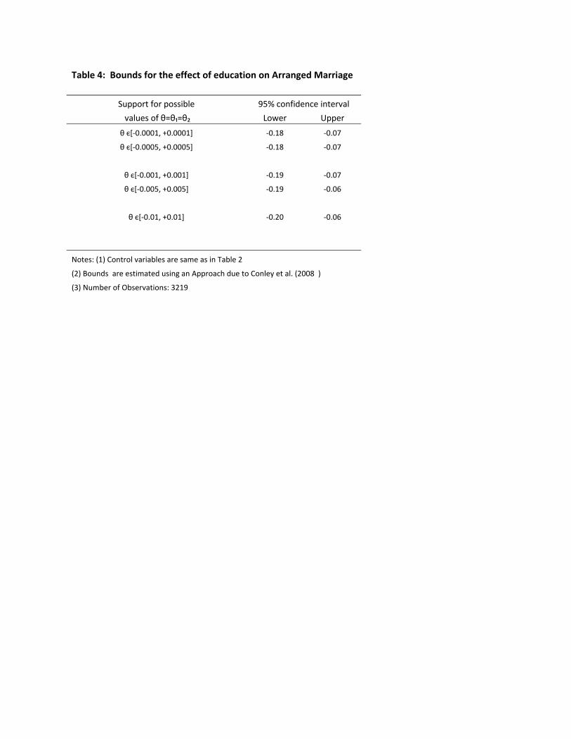
Table 4: Bounds for the effect of education on Arranged Marriage

Support for possible 95% confidence interval values of θ=θ₁=θ₂ Lower Upper

θ є[‐0.0001, +0.0001] ‐0.18 ‐0.07 θ є[‐0.0005, +0.0005] ‐0.18 ‐0.07

θ є[‐0.001, +0.001] ‐0.19 ‐0.07 θ є[‐0.005, +0.005] ‐0.19 ‐0.06

θ є[‐0.01, +0.01] ‐0.20 ‐0.06

Notes: (1) Control variables are same as in Table 2 (2) Bounds are estimated using an Approach due to Conley et al. (2008 )

(3) Number of Observations: 3219

Table 5: Gender, Education and Arranged Marriage

Dependent variable: Dummy for Arranged Marriage

Panel A: Female Sample



Years of schooling ‐0.74*** ‐

0.22*** ‐0.42*** ‐

0.15*** ‐0.17*** ‐0.17*** ‐0.17***

(‐5.16) (‐5.22) (‐14.14) (‐9.55) (‐3.82) (‐3.87) (‐3.86)

[0.00] [0.00] [0.00] [0.00] [0.00] [0.00] [0.00]

First Stage Residuals 0.70*** 0.20***




Hansen's J p value 0.91 0.91 0.91

Finlay‐Magnusson Weak IV Robust Inference, H₀: beta[Arranged: Years of Schooling] = 0

Linear IV IVProbit (Tests for Coefficients not for M.E)


CLR₂ 34.61 0.00 [‐.29,‐.10] 26.47 0.00 [‐.53,‐.43] AR₃ 34.87 0.00 [‐.34,‐.08] 27.27 0.00 [‐.53,‐.34]

Number of Observations:1716

Panel B: Male Sample



Years of schooling ‐0.27 ‐0.08 ‐0.28** ‐0.09* ‐0.05 ‐0.06* ‐0.06*

(‐1.55) (‐1.55) (‐2.39) (‐1.86) (‐1.54) (‐1.78) (‐1.80)

[0.12] [0.12] [0.02] [0.06] [0.12] [0.08] [0.07]

First Stage Residuals 0.22 0.06




Hansen's J p value 0.57 0.57 0.58

Panel B2: Finlay‐Magnusson Weak IV Robust Inference, H₀: beta[Arranged: Years of Schooling] = 0

Linear IV IVProbit (Tests for Coefficients not for M.E)


CLR₂ 3.89 0.07 [‐.18,‐.00] 2.39 0.15 [‐.75, .11] AR₃ 4.95 0.18 [‐.19,.02] 5.85 0.12 [‐.74, .11]

Number of Observations:1503

₁M.E. stands for Marginal Effects. M.E. are evaluated at the sample mean. ₂Conditional Likelihood Ratio Test, ₃ Anderson‐Rubin Test

Appendix

Table A‐1: Linear Probability Model Estimates

Dependent variable: Dummy for arranged marriage

(1) (2) (3) (4)

Years of schooling ‐0.02*** ‐0.02*** ‐0.02*** ‐0.01***

(‐6.91) (‐6.67) (‐6.67) (‐4.22)

[0.00] [0.00] [0.00] [0.00]

Other Controls

Age 0.00 0.00 0.00 0.00

Age squared 0.00 0.00 0.00 0.00

Age at marriage ‐0.02*** ‐0.02*** ‐0.02*** ‐0.02***

Married b. 1960 0.18*** 0.20*** 0.20*** 0.21***

Number of siblings 0.01* 0.00 0.00 0.00

Has no religion ‐0.06*** ‐0.05*** ‐0.05*** ‐0.04***

Met spouse in school ‐0.12*** ‐0.12*** ‐0.12*** ‐0.13***

Male 0.05*** 0.04*** 0.04*** 0.03**

Father is farmer 0.01 0.01 0.00

Father first born 0.00 0.00 0.00

Father's number of siblings 0.01*** 0.01*** 0.01***

Mother is farmer 0.02 0.02 ‐0.02

Mother is first born 0.01 0.01 0.01

Mother's number of siblings 0.01*** 0.01*** 0.01***

HH's Number of children ‐0.01

HH has brickwall 0.08*

HH access to information (tv, radio) ‐0.04**

HH's agricultural income ‐0.01

HH's wage ‐0.02***

Rural Dummy 0.06** Labor Market Opportunities₁ ‐0.14 ‐0.13 ‐0.13 ‐0.08

Sex Ratio 0.00 0.00 0.00 0.00

Constant 0.82** 0.62* 0.62* 0.56

R‐squared 0.17 0.18 0.18 0.19




*** p<0.01, ** p<0.05, * p<0.1

education and freedom of choice: evidence from arranged...

Documents