eduard musin (a9838) t879sn - theseus.fi

Eduard Musin (A9838)

T879SN

Adsorption Modeling

Bachelor’s thesis Environmental Engineering

June 2013

1

DESCRIPTION

Date of the bachelor's thesis

03.06.2013

Author(s)

Eduard Musin

Degree programme and option

Environmental Engineering

Name of the bachelor's thesis

Adsorption Modelling Abstract

In this study, adsorption was explored to remove toxic metals from wastewaters. The main

focus of the research work lies on adsorption process, which is described theoretically and

studied experimentally. Theoretical part involves studying of the adsorption concepts, ad-

sorbents and adsorption process modelling. Experimental part of the work was aimed to cre-

ate a condition which will allow examining the adsorption process by using adsorbents to

remove toxic metal from aqueous solution. The experiment was divided on analysing opti-

mum concentration and optimum time periods to remove Zn(II) and Cu(II) from aqueous

solution by using studied adsorbents. Secondly, the determination of pH values when adsor-

bents have the highest adsorption activity was required to study. The gathered data were

applied to model adsorption process via kinetic and isotherm adsorption models. The target

of research was reached: all results of experimental part were satisfactory to be described and

concluded by theory.

Subject headings, (keywords)

Adsorption, adsorbent, adsorbate, isotherm, kinetic, toxicology, metals, zeta potential, ICP Pages Language URN

54 + Appendices

English http://www.urn.fi/URN:NBN:fi:amk-2013122021992

Remarks, notes on appendices

Tutor

Aila Puttonen

Employer of the bachelor's thesis

Laboratory of Green Chemistry, Lap-peenranta University of Technology;

Mika Sillanpää, Evgenia Iakovleva

2

CONTENTS

1 INTRODUCTION ................................................................................................... 3

2 WASTEWATER TREATMENT TECHNOLOGY ............................................... 4

3 POLLUTION AND SOURCES .............................................................................. 6

4 TOXICOLOGY ....................................................................................................... 7

4.1 Essential and dangerous elements.................................................................. 7

4.2 Toxic metals ................................................................................................... 7

4.2.1 Zinc (Zn) ............................................................................................ 8

4.2.2 Copper (Cu) ....................................................................................... 9

5 BASICS CONCEPTS AND THEORY OF ADSORPTION .................................. 9

5.1 Adsorption mechanism ................................................................................ 10

5.2 Physisorption and chemisorption ................................................................. 11

6 ADSORPTION PROCESS MODELLING .......................................................... 13

6.1 Adsorption Kinetics ..................................................................................... 13

6.2 Adsorption Isotherms ................................................................................... 14

6.3 Zeta Potential ............................................................................................... 15

6.4 Adsorbents ................................................................................................... 16

7 ADSORPTION MODELING ............................................................................... 20

8 RESULTS AND DISCUSSION ........................................................................... 24

8.1 Optimum concentration of adsorbent .......................................................... 24

8.2 Adsorption time ........................................................................................... 25

8.3 Adsorption kinetics ...................................................................................... 27

8.4 Isotherm adsorption modelling .................................................................... 30

8.5 Zeta potential ............................................................................................... 33

9 CONCLUSION ..................................................................................................... 35

BIBLIOGRAPHY ........................................................................................................ 36

APPENDICES

1. Data from experiments

2. Figures

3

1 INTRODUCTION

It is commonly known that Earth is covered by approximately 70% of water, where only

2,5-3% is unleavened water. The large amount of drinkable water is in hard aggregate

condition as ice. Eventually, we have less than 1% of fresh water from those 2,5-3%

[1]. This amount of drinkable water should be distributed on the growing population of

7 billion inhabitants on the Earth. In accordance to the size of the planet and the amount

of inhabitants, the water is available for all of us. However, if the amount of pollutions

caused by the activities of the modern world is taken into account, the situation becomes

more complicated. Nowadays water pollution is the main agenda of different countries.

Surplus of wastewater and lack of pure water pushes government and citizens to pay

more for a sip of fresh water and use it rationally. Water treatment technologies help to

decrease and sometimes completely illuminate a harmful effect on the environment, and

it helps to make equilibrium in natural water cycle. [1].

Water can be polluted naturally or anthropogenically. Therefore, a selection of

wastewater treatment methods is an essential question which is related to the types of

wastewater. Generally, wastewater can be divided on domination of organic compound

or inorganic matter in it. This research studies inorganic compounds removal from

wastewater. In the role of contaminants are toxic metals which are dangerous for the

environment and deadly poisonous for humans and animals. Most of the point sources

of toxic metals are fuel industry, machinery, traffic, ferrous metallurgy, non-ferrous

metallurgy, mining industry, chemical industry, electroplating etc. Contaminants in

wastewaters might be different and complex substances. [1]. Therefore, a determination

of a method of wastewater treatment for a certain particular case is observed individu-

ally. The capacity of all methods of wastewater treatments is essential to analyse theo-

retically and technically through experiments, which give plenty of data, which help to

realize a contaminant reduction dynamics from wastewaters. However, most of those

methods are suffering from drawbacks, such as high consumption of reagent and en-

ergy, high capital, high operational costs and the resulting sludge which is difficult to

dispose of [2]. Consequently, it is necessary to use a method which might be promptly

implemented but also cost-effective. In this study adsorption was chosen as a good way

for industrial wastewater treatment and removal of toxic metal, because adsorption has

4

many benefits compared to other methods, such as lower operating cost and simplicity

in utilization. The main target of this research work was to study adsorption process

theoretically and practically. [2, 3].

Study of adsorption was performed in Laboratory of Green Chemistry, which is a de-

partment of Lappeenranta University of Technology. The laboratory is located in Mik-

keli. The Head of the Laboratory is Professor Mika Sillanpää. Laboratory of Green

Chemistry focuses on studying technologies, such as adsorption, analytics, online mon-

itoring, advanced oxidation processes, electrokinetics and electrochemical technolo-

gies. [2].

2 WASTEWATER TREATMENT TECHNOLOGY

The wastewater treatment technologies are aimed to decrease the harmful effect for the

environment by organic and inorganic contaminants in water. Treated wastewater

should be able to be discharged into the environment or to be used by industries without

negative consequences. The wastewater treatment technologies have strong future per-

spectives which create challenging condition in water treatment development. There-

fore, wastewater treatment technologies are on high priority among other technologies.

Wastewater treatment technologies can be divided on active and passive methods. The

main difference between passive and active water treatment systems is that passive ones

use naturally available energy sources, such as photosynthesis, microbial metabolic en-

ergy and/or topographical gradient, compared to active ones, which require external

sources of energy as electricity. [4].

Active and passive methods

The list of well-known active methods includes neutralization, filtration, ion exchange,

electrodialyses, solvent extraction, freeze separation and adsorption (Table 1). The word

“active” implies that active methods require a lot of maintenance and external energy

to carry a treatment process. Passive wastewater treatment methods are less efficient

than active wastewater treatment methods and usually used as addition to active meth-

ods. Passive methods include constructed wetlands, limestone drains and reactive bar-

riers (Table 1). Passive wastewater treatment requires less of technical maintenance

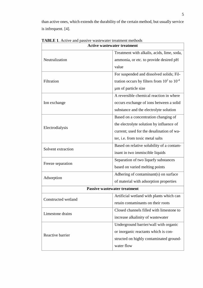
5

than active ones, which extends the durability of the certain method, but usually service

is infrequent. [4].

TABLE 1. Active and passive wastewater treatment methods

Active wastewater treatment

Neutralization

Treatment with alkalis, acids, lime, soda,

ammonia, or etc. to provide desired pH

value

Filtration

For suspended and dissolved solids; Fil-

tration occurs by filters from 102 to 10-4

µm of particle size

Ion exchange

A reversible chemical reaction in where

occurs exchange of ions between a solid

substance and the electrolyte solution

Electrodialysis

Based on a concentration changing of

the electrolyte solution by influence of

current; used for the desalination of wa-

ter, i.e. from toxic metal salts

Solvent extraction Based on relative solubility of a contam-

inant in two immiscible liquids

Freeze separation Separation of two liquefy substances

based on varied melting points

Adsorption Adhering of contaminant(s) on surface

of material with adsorption properties

Passive wastewater treatment

Constructed wetland Artificial wetland with plants which can

retain contaminants on their roots

Limestone drains Closed channels filled with limestone to

increase alkalinity of wastewater

Reactive barrier

Underground barrier/wall with organic

or inorganic reactants which is con-

structed on highly contaminated ground-

water flow

6

In this study, adsorption is chosen as a method of toxic metals removal from aqueous

phase because it has significant benefits among other wastewater treatment methods.

On the one hand, operating costs are low and utilization is simple; on the other hand,

adsorption is a highly efficient method in removing very low levels of toxic metals from

dilute solutions. High selectivity, minimum production of by-products such as chemical

sludge, and regeneration ability are the most valuable point for adsorption. [3, 5].

3 POLLUTION AND SOURCES

Transportation of heavy metals into the environment occurs as a result of natural pro-

cesses of distribution. Nevertheless, the anthropogenic emissions of heavy metals take

even stronger position compare to natural sources. [1, 6].

Sources of toxic metals

The significant amount of heavy metals comes from [1]:

Fuel industry and fuel machinery, such as V, Hg, Pb

Traffic Pb, Hg, V

Ferrous metallurgy and non-ferrous metallurgy Fe, Cr, Cu, Mo

Mining industry Cu, Zn, Fe

Chemical industry Zn, Cd

Electroplating Zn, Cu

Rubber, plastic and wood industries Se, Pb

From the whole list of heavy metals from industrial units, the large amounts of Pb, Zn

and Ni come into the environment in comparison with others (respectively over 33, 13

and 6 thousand tons/year in the countries of West Europe). Currently, anthropogenic

flows of Pb, Hg, Cd, Ni, V, As, Sb and Se prevail over natural sources. However, the

anthropogenic flow of toxic metals into the environment is based on order [4]:

Cd>Pb>As>Zn>Ni>Co>Se

All toxic metals are dangerous, especially when occupational exposure limits are ex-

ceeded, for example V, Co, Ni, Cu, Zn, Cd, Pb, Zn, As, Se are the most dangerous with

oxidation number two (II). Hg and Cr with all oxidation numbers are dangerous. [6]

7

Nevertheless, for all industries, whose activity and/or by-products consist of toxic met-

als, exist directives and regulations aimed to control the emission level. The purification

of wastewaters is implemented at the source of pollution. EU has directives related to

wastewater treatment and discharge, such as “Council Directive 91/271/EEC concern-

ing urban waste-water treatment” which aimed to manage urban and industrial units’

wastewaters discharge into the environment. [7].

4 TOXICOLOGY

Collocation “heavy metals” was included into scientific lexicon at the end of 1960 th.

Also it is named as “toxic metals”. From one point of view, the toxic metals are deadly

poison for living organisms but, on the other hand, many of them are essential for vari-

ous living organisms. [6].

4.1 Essential and dangerous elements

Different techniques of chemical analyses and study of biochemical processes allowed

determining a biological importance of many elements. All in all, 80 chemical elements

including heavy metals such as Mn, Ni, Cu, Cr, V and Zn were identified in the living

cells. All of them together with Fe, Co and Mo are a part of the enzymes or enzyme

activators. [6]. The individual demand of heavy metals is low, for example in the body

of adult a general concentrations of Zn is 12-16 mg, Cu 0.9-2.2 mg, Ni 100-300 µg, Fe

10-18 mg. The excess amounts of heavy metals from natural concentration levels can

be a reason of serious disturbances of metabolism. Chemical eco-toxicology pays more

attention to those toxic metals, which are amenable to replacing essential elements, bio-

accumulating (cumulative effect in the organism) and/or ecological magnification (it is

a process of increasing of a chemical element(s) concentration in a living body during

a transition from the lower trophic levels (food chain position of an organism) of a cer-

tain ecosystem to a higher one. [4, 6]

4.2 Toxic metals

The main importance in toxic metals analyses is to study the element’s solubility, es-

sentiality, physiological effect, toxicokinetics, toxicity and nature of a certain metal. For

this research work, Zn and Cu were observed. These metals are the most common in

8

wastewaters of many industries [6]. Allowable EU standard concentrations of Zn and

Cu in wastewater from non-domestic sources [8]:

Zn ≥ 5 g/l

Cu ≥ 1 g/l

Excessive amounts of toxic metals found in wastewater in high than allowable EU

standard concentrations can put a stop to an activity of a certain industry [8].

4.2.1 Zinc (Zn)

Zinc is a chemical element which has a molar mass 65.38; atomic number is 30 in the

periodic table with the chemical symbol Zn. All salts of zinc are well dissociated in

water. [6].

Essentiality and physiological effect

Zinc is nutritionally essential trace metal and might be labelled as ubiquitous in the

environment. Zinc is presented in soil, water, air and most foodstuffs. Deficiency of

zinc may cause serious health problems. More than 200 metalloenzymes (enzymes that

require metals to carry out normal functioning of metalloproteins) require zinc as a co-

factor, non-protein chemical compound aimed for the protein’s biological activity. Zinc

takes part in many chemical-biologic processes. [6].

Toxicokinetics

Daily recommended dose for adults of zinc in average is approximately 12-16 mg. The

natural sources of zinc are usually from food, such as vegetables, fruits and meat. Ac-

cording to essentiality of this element the recommended dose should be covered for the

normal vital activity. [6].

Toxicity

All zinc salts are highly toxic to humans and animals. Chlorides (ZnCl2), sulphates

(ZnSO4), and zinc oxide (ZnO) can cause severe poisoning of a body. The reason of

9

high toxicity is toxic ions of Zn2+. 1g of zinc sulphate ZnSO4 is enough to cause a severe

poisoning. ZnSO4 poisoning leads to anaemia, growth retardation and infertility. [6].

4.2.2 Copper (Cu)

Copper is a chemical element which has a molar mass 63.55; atomic number is 29 in

the periodic table with the chemical symbol Cu. All salts of copper are well dissociated

in water. [6].

Essentiality and physiological effect

Copper is widely spread in nature and is a nutritionally essential element. Copper is a

component of all living cells and associated with many oxidative processes. It is an

essential component of metalloenzymes which take part in haematopoiesis. [6].

Toxicokinetics

For adults the daily intake of copper is varies between 0.9-2.2 mg. The natural sources

of copper are vegetables, fruits and meat. Copper is involved in the formation and re-

generation of bone tissue. It increases the activity of pituitary hormones, increases the

body's defence (for the strengthening of the immune system), and increases the antitoxic

function of the liver. Copper has bactericidal properties. [6].

Toxicity

A systematic intake of copper salts, most frequently copper sulphate, may cause hepatic

necrosis and death. According to toxicity of copper, it can be pointed that risks to human

health from a lack of copper in a body is many times higher than a risk of its excess.

[6].

5 BASICS CONCEPTS AND THEORY OF ADSORPTION

The main target for this research work was to study adsorption process theoretically and

practically. The concept of adsorption, dynamics of adsorption development, types of

adsorption, study of adsorbents, treatment capacity of adsorption and adsorption process

10

modelling are described in the theoretical part. The practical part contains study of ad-

sorbents, determination of adsorbent concentrations for contaminant removal, prepara-

tion of adsorbate solution, initializing a treatment process, sampling, solution analysis,

data analysis and adsorption modelling. The most significant part is the modelling of

adsorption process. Modelling is based on isotherms of adsorption, adsorption kinetic

models and zeta potential. [2, 3].

Adsorption is a surface phenomenon where adsorbent is a substance which adheres an-

other substance on its surface. A substance which accumulates on the surface of adsor-

bent is named adsorbate. Adsorption might be chemical or physical process, or combi-

nation of those, which occurs at the common boundary of two phases, such as liquid-

solid, gas-solid, gas-liquid or liquid-liquid. [9]. By other words, adsorption is a change

in concentration of a certain substance (i.e. contaminant) at an interface where an initial

concentration is decreased. Historically, adsorption has been first observed by

C.W.Scheele in 1773 for gases. Lowitz has continued observation of experiments in

1785 for solutions. Currently, adsorption is actively studied by many institutes around

the world, for example Laboratory of Green Chemistry, which is a department of Lap-

peenranta University of Technology ruled by Professor Mika Sillanpää. [2, 10].

Adsorption has importance for industries which work with gas, petroleum, air and water

purification. Adsorption is applied for purifications of organics and SO2 from gas phase.

Also water can be extracted from O2, CH4, N2, additionally NOx can be excreted from

N2. Adsorption is also used for gas separations, such as N2 from O2, acetone and C2H2

from vent stream, and CO, CH4, CO2, N2, Ar from hydrogen. In the liquid phase, ad-

sorption is applied, for example, for organic and inorganic removal, and decolouriza-

tion. [11]

5.1 Adsorption mechanism

The classical mechanism of adsorption is divided into three steps (Fig.1): a) diffusion

of adsorbate to adsorbent surface, b) migration into pores of adsorbent c) monolayer

build-up of adsorbate on the adsorbent. Fig.1 presents the process of adsorbate distribu-

tion. Step 1 occurs diffusion of adsorbate on the adsorbent surface by intermolecular

forces between adsorbate and adsorbent. The second step involves migration of adsorb-

11

ate into pores of adsorbent. During the last step, when the adsorbate’s particles are dis-

tributed on the surface and filled up the volume of pores, particles of adsorbate are

building up the monolayer of reacted molecules, ions and atoms to the active sites of

adsorbent. [2, 3].

FIGURE 1. Three steps of adsorption mechanism: a) diffusion of adsorbate to adsor-

bent surface b) migration into pores of adsorbent c) monolayer build-up of adsorbate on

adsorbent [11]

5.2 Physisorption and chemisorption

The nature of adsorption depends upon the forces which act between adsorbent and

adsorbates. The adsorption forces are a key factor in defining whether the adsorption is

physical or chemical. Occasionally, it is complicated to identify what type of adsorption

is predominating in a certain situation. Sometimes it might be a combination of chemi-

sorption and physisorption. [5, 9]

Physisorption

Physical adsorption is reversible and rapid. Molecules are holding to the surface by van

der Waals forces of attraction (intermolecular forces and interatomic interactions with

the energy of 10-20 kJ/mol). Therefore, the lack of interaction energy may break the

a) b) c)

12

bond between adsorbent and adsorbate, for example by mechanical movement of the

interface. Consequently, the most valuable parameters for physisorption are the pore

size, pore structure, pore volume, and surface area. Physisorption prevails at low tem-

peratures, and activation energy is 5-10 Kcal/mol. [5, 9]

A mechanism of hydrogen storage on the surface of highly porous material is shown in

Figure 2. The molecules of hydrogen accumulate at the surface of the porous material

without reacting chemically with it. [12]

FIGURE 2. Mechanism of hydrogen storage by physisorption [12]

Chemisorption

A specific surface area of phases, types of active sites, number of active sites, and sta-

bility of active sites are predominantly valuable for chemisorption. Chemical adsorption

occurs as a result of chemical reaction between molecules and atoms of the adsorbate

and adsorbent. Chemisorption is irreversible because chemically adsorbed molecules

are not able to move on the surface of within interface. The main advantages are high

selectivity of separation and the ability to treat exceptionally small concentrations of

solute. Chemisorption accelerates by elevated temperature where activation energy var-

ies between 10-100 Kcal/mol. [5, 9]

A mechanism of hydrogen storage by using chemisorption onto certain metals was

taken as example. In figure 3 (a) hydrogen molecules attached on the surface of the

13

material. Then molecules split into separate atoms (Fig.3 (b)). The hydrogen atoms dis-

tribute randomly in the structure of material (Fig.3 (b)). Finally, hydrogen compounds

adopt an ordinary arrangement and form ionic, covalent or metallic bonds with the metal

atoms (Fig 3 (c)). [12]

FIGURE 3. Mechanisms of hydrogen storage by chemisorption. Modified from [12]

6 ADSORPTION PROCESS MODELLING

Adsorption process modelling helps to identify the removal efficiency of adsorbent.

Adsorption modelling is applied to describe the experimental data by using adsorption

isotherm and kinetic models. Additionally zeta potential is applied for analysing ad-

sorption process. [11]

6.1 Adsorption Kinetics

The kinetic equations of the chemical reaction show the dependence of the reaction rate

on the concentrations of the reactants. The kinetic equation of chemical reaction is de-

termined experimentally by using gathered data from the experiment. The study of ad-

sorption kinetics is important because it provides valuable information and describes

the mechanism of the reaction. [2]

Adsorption kinetics helps to determine the overall rate of the adsorption process. The

mechanism of adsorption process is investigated by kinetic equations, for example zero-

, first- and second-order, pseudo-first- and pseudo-second-order. [4, 13] In this study

14

pseudo-first- and pseudo-second-order reactions were observed, as the most common

cause for adsorption modelling. [13]

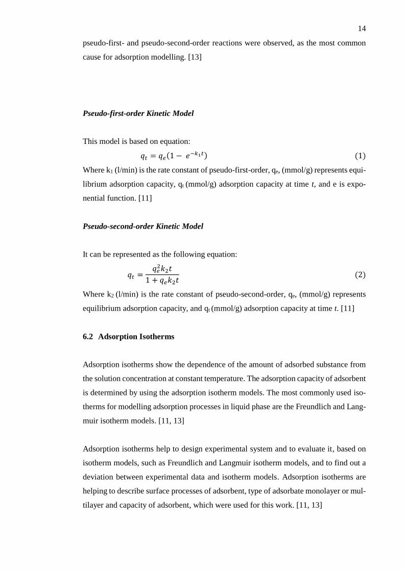
Pseudo-first-order Kinetic Model

This model is based on equation:

𝑞𝑡 = 𝑞𝑒(1 − 𝑒−𝑘1𝑡) (1)

Where k1 (l/min) is the rate constant of pseudo-first-order, qe, (mmol/g) represents equi-

librium adsorption capacity, qt (mmol/g) adsorption capacity at time t, and e is expo-

nential function. [11]

Pseudo-second-order Kinetic Model

It can be represented as the following equation:

𝑞𝑡 =𝑞𝑒

2𝑘2𝑡

1 + 𝑞𝑒𝑘2𝑡 (2)

Where k2 (l/min) is the rate constant of pseudo-second-order, qe, (mmol/g) represents

equilibrium adsorption capacity, and qt (mmol/g) adsorption capacity at time t. [11]

6.2 Adsorption Isotherms

Adsorption isotherms show the dependence of the amount of adsorbed substance from

the solution concentration at constant temperature. The adsorption capacity of adsorbent

is determined by using the adsorption isotherm models. The most commonly used iso-

therms for modelling adsorption processes in liquid phase are the Freundlich and Lang-

muir isotherm models. [11, 13]

Adsorption isotherms help to design experimental system and to evaluate it, based on

isotherm models, such as Freundlich and Langmuir isotherm models, and to find out a

deviation between experimental data and isotherm models. Adsorption isotherms are

helping to describe surface processes of adsorbent, type of adsorbate monolayer or mul-

tilayer and capacity of adsorbent, which were used for this work. [11, 13]

15

Langmuir Isotherm Model

According to the Langmuir model, adsorption occurs uniformly on the active sides of

the adsorbent. The Langmuir isotherm model is described by the following formula:

𝑞𝑒 =𝑞𝑚𝐾𝐿𝐶𝑒

1 + 𝐾𝐿𝐶𝑒 (3)

Where, qe (mmol/g) is equilibrium adsorption capacity (mg/l), Ce is equilibrium concen-

tration (mg/l), qm is maximum adsorption capacity (mg/g), and KL (l/mg) is the Lang-

muir’s constant. [2, 5, 11]

Freundlich Isotherm Model

The Freundlich isotherm is an empirical model that is based on adsorption on a hetero-

geneous surface (surface with varying properties i.e. any surface properties are distrib-

uted unevenly, for example surface energy is different at certain points). This is appli-

cable to a non-ideal sorption as well as a multilayer sorption process. The Freundich

model is given by the following equation [11, 13]:

𝑞𝑒 = 𝐾𝐹𝐶𝑒1/𝑛𝐹 (4)

Where KF is Freundlich affinity constant (based on (mmol/g)/(l/mmol)nF), nF is the

Freundlich heterogeneity factor, qe (mmol/g) is equilibrium adsorption capacity (mg/l),

Ce is equilibrium concentration (mg/l), and 1/nF is the heterogeneous factor. [11, 13]

6.3 Zeta Potential

Zeta potential is a measure of the magnitude of the electrostatic interrelation (repulsion

or attraction) between particles. Analysing zeta potential helps to get a clear picture of

mechanisms in cases of flocculation, aggregation or dispersion. [11]

Zeta potential helps to determine adsorption properties when adsorbent’s particles are

mixed in liquids. Particles in liquids or suspensions are usually charged. A surface of

an adsorbent particle is negatively or positively charged, and it is surrounded by ions

with the opposite charge. Therefore, a charge of a particle is essential in adsorbent anal-

yses to evaluate adsorbent potential. Zeta potential analysis helps to identify an isoelec-

tric point of adsorbent. Isoelectric point is a pH value at which adsorbent does not have

a charge to attract adsorbate. [11]

16

Figure 4 shows dependency of zeta potential (mV) at different pH values. At pH 6 the

curve does not have any charge (mV); this is named as isoelectric point. If zeta potential

is negatively or positively high it means that attraction charge is stable and can retain

ions stronger.

FIGURE 4. Zeta potential, isoelectric point

6.4 Adsorbents

Adsorbent - a substance with the adsorption properties. The important properties of ad-

sorbent are selectivity, high capacity, chemical and thermal stability, low solubility in

the carrier solvent, regeneration ability, physical stability and low cost. [3, 9]

Activated carbon

Activated carbon (Fig. 5) is the well-known adsorbent which is widely used in many

industries, such as water treatment and medical production. It has exceptionally strong

adsorption properties and complicated structure. Activated carbon can be produced by

physical or chemical activation from material such as coal, lignite, nutshells, peat, wood

and petroleum pitches. [2, 14, 15]

60

20

0

-60

40

-40

-20

Zeta

Po

ten

tial

(m

V)

pH

11 10 9 8 2 3 4 5 6 7

Stab

le

Stab

le

Isoelectric point

17

FIGURE 5, Activated carbon, a) milled carbon which is powder, b) granulated active

carbon [16]

Zeolite

Zeolites (Fig.6) are complex aluminosilicate containing oxides of alkali and alkaline

earth metals. Natural and synthetic zeolites have a frame structure which give unique

adsorption properties. Zeolite is widely used adsorbent for different purposes. It is ap-

plied for unsurpassed gas driers and cleaners, organic and inorganic compound removal

from liquids and gases. Zeolite might be natural, modified natural or synthetic. Physi-

cochemical properties of zeolite are thermal stability, high adsorption potential at low

temperatures, and extremely powerful sorption capacity to extract water from gases. [2,

17]

FIGURE 6. Zeolite, a) synthetically manufactured in granules, b) crushed natural zeo-

lite and c) mineralized zeolite [17]

a

b

a

b c

18

Activated alumina

Activated alumina is a refractory compound of Al2O3 (Fig. 7). Activated alumina is ac-

tive amorphous oxide with different adsorption properties. It is hydrophilic and has

strongly developed pore structure. It is produced from aluminium hydroxide by dehy-

drating. It is used in purification of liquids and gases to remove, for example fluoride,

arsenic, selenium. Also in industry it is used as drier for natural gas and other gases in

gaseous and liquid phases. Important properties are thermal stability, easy manufactur-

ing and regeneration. [2, 18, 19]

FIGURE 7. Activated alumina, manufactured in spheres form [18]

Silica gel

Silica gel (Fig.8) is a solid adsorbent which forms as spherical translucent-matte beads

in sizes from 3 to 8 mm. The structure of silica gel is highly porous formed by tiny

spherical particles. The chemical composition is SiO2. Silica gel is used to adsorb water

vapour and organic solvents and non-polar liquids. In gas and liquid chromatography it

is used for the separation, for example alcohols, amino acids, vitamins, antibiotics.

Large-pore silica gels are used as catalyst supports. [2]

19

FIGURE 8. Spherical transparent beads of silica gel [20]

Chitosan

Chitosan (Fig. 9) is organic adsorbent, which is made from crab-shell chitin. It has high

efficiency of toxic metals removal from wastewater. Chitosan is surprisingly cheap ad-

sorbent with its strong adsorption properties. Chitosan can adsorb 60 different metal

ions from wastewater, such as Be(II), Mn(II), Co(II), Ni(II), Cu(II), Zn(II), Ga(III),

Y(III), Ag(I), Cd(II), In(III), Pb(II), Bi(III), Th(IV). [2, 21]

FIGURE 9. Chitosan produced as flakes (a) and as powder (b) [22]

The list of commonly known and widely used adsorbents with strong adsorption prop-

erties can include biosorbents which are based on physicochemical process where con-

taminant settles on cellular structure. Sources of biosorbents are agricultural residues,

algae plants, microbial species, yeasts and fungi. [23]. Municipal sewage sludge and

a

b

20

industrial wastes can be considered as low-cost adsorbents with powerful adsorption

properties which can be used for wastewater treatment purposes. [2]

Not all adsorbents have naturally strong sorption capacity to remove contaminants.

Some of them cannot work as adsorbents without pre-treatment. Pre-treatment is mod-

ification which might be chemical, mechanical and/or thermal. [10]

7 ADSORPTION MODELING

The experimental study of adsorption process was organized by Laboratory of Green

Chemistry. Study of adsorbents was focused on adsorbent retention time, adsorbent sta-

bility, adsorbent concentration, a contact time of adsorbent and adsorbate, dependency

on adsorption capacity of pH.

The target of the modelling was to identify the adsorption isotherm and kinetic models

which can describe the experimental data gathered from ICP (inductively coupled

plasma optical atomic emission spectrometry) analysis. Adsorption process modelling

was based on Langmuir’s and Freundlich’s isotherm models. Pseudo-first-order and

pseudo-second-order kinetic models were applied to study kinetics. Zeta potential was

used to determine an isoelectric point of adsorbents.

Adsorption process modelling is a complex task which was separated for this work on:

1) Identifying the minimum concentration of adsorbent in the solution with maxi-

mum adsorption capacity of toxic metal removal

2) Identifying time periods when the chosen concentration of adsorbent in the so-

lution is the most efficient for toxic metal removal

3) Modelling adsorption process through adsorption isotherm and kinetic models,

and zeta potential determination

Experimental work

Preparation of experiment was based on batch method for analysing adsorption process.

This method requires placing together adsorbent and adsorbate in the same space with

constant mixing. Inductively coupled plasma optical atomic emission spectrometry

21

(ICP-OES) model iCAP 6000 Series (Fig. 30, 31) was applied to analyse the concentra-

tion of metals in solutions. Gathered data from ICP was used for adsorption isotherm

and kinetic modelling. Isoelectric point (pH value when a certain molecule or surface

carries no electric charge) was measured by Zetasizer Nano Series model ZEN 3600

(Fig. 32, 33).

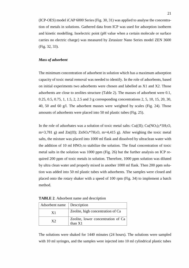
Mass of adsorbent

The minimum concentration of adsorbent in solution which has a maximum adsorption

capacity of toxic metal removal was needed to identify. In the role of adsorbents, based

on initial experiments two adsorbents were chosen and labelled as X1 and X2. Those

adsorbents are close to zeolites structure (Table 2). The masses of adsorbent were 0.1,

0.25, 0.5, 0.75, 1, 1.5, 2, 2.5 and 3 g corresponding concentrations 2, 5, 10, 15, 20, 30,

40, 50 and 60 g/l. The adsorbent masses were weighted by scales (Fig. 24). Those

amounts of adsorbents were placed into 50 ml plastic tubes (Fig. 25).

In the role of adsorbates was a solution of toxic metal salts: Cu((II); Cu(NO3)2*3H2O,

m=3,781 g) and Zn((II); ZnSO4*7H2O, m=4,415 g). After weighing the toxic metal

salts, the mixture was placed into 1000 ml flask and dissolved by ultraclean water with

the addition of 10 ml HNO3 to stabilize the solution. The final concentration of toxic

metal salts in the solution was 1000 ppm (Fig. 26) but the further analysis on ICP re-

quired 200 ppm of toxic metals in solution. Therefore, 1000 ppm solution was diluted

by ultra clean water and properly mixed in another 1000 ml flask. Then 200 ppm solu-

tion was added into 50 ml plastic tubes with adsorbents. The samples were closed and

placed onto the rotary shaker with a speed of 100 rpm (Fig. 34) to implement a batch

method.

TABLE 2. Adsorbent name and description

Adsorbent name Description

X1 Zeolite, high concentration of Ca

X2 Zeolite, lower concentration of Ca

than X1

The solutions were shaked for 1440 minutes (24 hours). The solutions were sampled

with 10 ml syringes, and the samples were injected into 10 ml cylindrical plastic tubes

22

(Fig. 29) through filters to purify sediment from the solution before ICP analysis (Fig.

28).

For ICP calibration, the calibration solutions at concentrations in 5, 10, 25, 50 and 100

ppm of Cu(II) and Zn(II) were prepared. The calibration solutions were diluted from

1000 ppm of commercial standard solutions bought from Romil LTD. The concentra-

tions dilution for calibration solutions were based on the following formula:

𝐶1𝑉1 = 𝐶2𝑉2 (5)

ICP analysis was used to determine the toxic metal concentrations in the solution with

different amounts of adsorbents after a certain period of time (1440 minutes). When the

samples and calibration solutions were placed on ICP’s auto sampler (Fig. 10), the last

step was to prepare ICP programme on the computer where studied toxic metals’ wave-

lengths were adjusted individually. The results were delivered into Excel sheets.

FIGURE 10. AutoSampler ASX-260, synchronized with iCAP 6000 Series

Time for metal removal

The same technique of preparation and measuring was applied with the most efficient

mass of adsorbent to identify an ideal adsorption time to remove toxic metals from

aqueous solution. The main importance of this step of measurements were identifying

time periods when a chosen concentration of adsorbent in the solution is the most effi-

cient for toxic metal removal. Time periods for sampling were 30, 60, 120, 180, 240,

300, 360, 420, 480, 720 and 1440 minutes from the starting moment.

23

ICP analysis was used to determine the toxic metal concentrations at constant concen-

tration of adsorbent in the solution after certain periods of time. The gathered data from

ICP were delivered into Excel file.

Zeta-potential and titration

Isoelectric points and zeta potential of the adsorbents were determined by using

Zetasizer Nano. For the experiment, 1,5 g of the adsorbents were weighted, and placed

into 50 ml plastic tubes. 50 ml of ultra clean water was added into plastic tubes with

adsorbents X1 and X2, and properly mixed by magnet stirrer (Fig. 27) for 5 minutes.

Zeta potential determination is done by titration. An initial pH of the solutions was im-

portant to be identified before measurements. Solution of X1 became alkaline and solu-

tion of X2 became acidic in water. Consequently, for a proper titration and identification

of the isoelectric points and zeta potential, pH value is important to know in advance.

The pH determination was made by pH meter (Fig. 27) and values of initial pH of so-

lutions are shown on Table 3. Thereafter the titrants were prepared based on the scheme:

Alkaline solutions were titrated by HCL (1, 0.1 and 0.001 M)

Acidic solutions were titrated by NaOH (1, 0.1 and 0.001 M)

TABLE 3. Adsorbent pH concentration of 30g/l of adsorbent dissolved in water

Adsorbent name pH

X1 8,529

X2 3,834

Before titration, to define zeta potential in the pH range 1-10:

X1 had an addition of NaOH until 9,5

X2 had an addition of HCl until 1,8

Eventually, the gathered data were received in graph format.

24

Modelling adsorption

All gathered data from ICP analyses (Tables 4, 6 and 8) were used to form adsorption

isotherm and kinetic models. Calculations were performed in Excel programme based

on adsorption isotherm and kinetic equations.

8 RESULTS AND DISCUSSION

In this research, the main targets were to analyse the minimum concentration of adsor-

bent in the solution with maximum adsorption capacity for toxic metal removal and

identifying time periods when a certain concentration of adsorbent in the solution is the

most efficient for toxic metal removal. It helps to evaluate the demand on adsorbent in

a certain case for the further rational usage of it and to decrease expenses. Gathered

experimental results can be used for large scale adsorption process designing. Another

target was to model adsorption process through adsorption isotherm and kinetic models,

and zeta potential determination. The results from these experiments can describe the

behaviour of adsorbent in definite condition, its stability, surface area and ability to

adsorb.

8.1 Optimum concentration of adsorbent

The efficiency of adsorbents X1 and X2 for removal of toxic metals from the solution

were analysed by ICP, which gave a clear data about how the concentration of adsorbent

is influencing on removing of toxic metals (Fig. 11). The most efficient amount of both

adsorbents to remove Cu(II) and Zn(II) was 50 g/l in Figure 11. This concentration can

remove 85% of studied toxic metal from solution by adsorbent X1 and 99,5% by adsor-

bent X2. In comparison between 50 g/l and 60 g/l of both adsorbents, they have similar

toxic metal removal dynamics from the solution. Consequently, 50 g/l is an optimum

concentration of adsorbent in solution for toxic metals removal.

25

FIGURE 11. Adsorbent capacity at different adsorbent concentrations in solution for

toxic metals removal

8.2 Adsorption time

For the second step of measurements by ICP, adsorbent’s efficiency was measured on

concentration 50 g/l with different time periods: 30, 60, 120, 180, 240, 300, 360, 420,

480, 720 and 1440 minutes. Figures 12 and 13 were built up based on removal capacity

of adsorbents at the certain sampling times. In Figure 12 adsorption of Zn(II) by adsor-

bent X1 goes rapidly at first 120 minutes with good removal capacity which equals 84%

at 2,4 pH. After this time, desorption of Zn(II) into the solution takes place in the reac-

tion by the substitution reaction of Zn(II) by Cu(II). Where removal of Zn(II) decreases

to 64% at 4,7 pH, then removal capacity for Zn(II) remains constant. Removal of Cu(II)

from the aqueous solution starts slower than Zn(II) and moderately rises until 93% at

5,4 pH, then removal capacity becomes constant.

0

10

20

30

40

50

60

70

80

90

100

0 10 20 30 40 50 60 70

Rem

ova

l, %

C, g/l

Concentration for metal removal

X1, Cu & Zn, %

X2, Cu & Zn, %

26

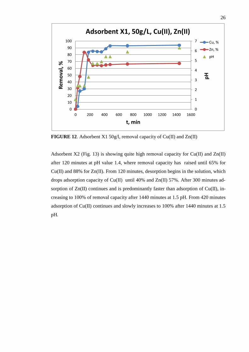
FIGURE 12. Adsorbent X1 50g/l, removal capacity of Cu(II) and Zn(II)

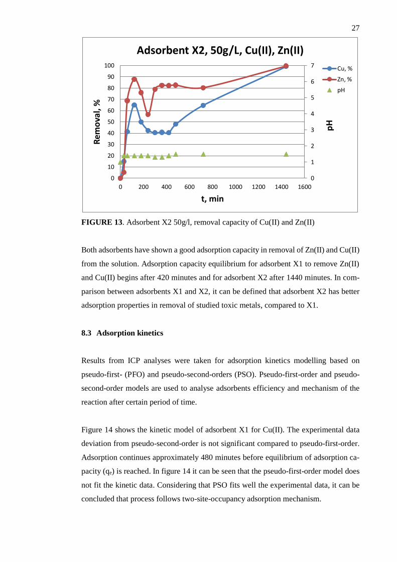
Adsorbent X2 (Fig. 13) is showing quite high removal capacity for Cu(II) and Zn(II)

after 120 minutes at pH value 1.4, where removal capacity has raised until 65% for

Cu(II) and 88% for Zn(II). From 120 minutes, desorption begins in the solution, which

drops adsorption capacity of Cu(II) until 40% and Zn(II) 57%. After 300 minutes ad-

sorption of Zn(II) continues and is predominantly faster than adsorption of Cu(II), in-

creasing to 100% of removal capacity after 1440 minutes at 1.5 pH. From 420 minutes

adsorption of Cu(II) continues and slowly increases to 100% after 1440 minutes at 1.5

pH.

0

1

2

3

4

5

6

7

0

10

20

30

40

50

60

70

80

90

100

0 200 400 600 800 1000 1200 1400 1600

Rem

ova

l, %

t, min

Adsorbent X1, 50g/L, Cu(II), Zn(II)

Cu, %

Zn, %

pH

pH

27

FIGURE 13. Adsorbent X2 50g/l, removal capacity of Cu(II) and Zn(II)

Both adsorbents have shown a good adsorption capacity in removal of Zn(II) and Cu(II)

from the solution. Adsorption capacity equilibrium for adsorbent X1 to remove Zn(II)

and Cu(II) begins after 420 minutes and for adsorbent X2 after 1440 minutes. In com-

parison between adsorbents X1 and X2, it can be defined that adsorbent X2 has better

adsorption properties in removal of studied toxic metals, compared to X1.

8.3 Adsorption kinetics

Results from ICP analyses were taken for adsorption kinetics modelling based on

pseudo-first- (PFO) and pseudo-second-orders (PSO). Pseudo-first-order and pseudo-

second-order models are used to analyse adsorbents efficiency and mechanism of the

reaction after certain period of time.

Figure 14 shows the kinetic model of adsorbent X1 for Cu(II). The experimental data

deviation from pseudo-second-order is not significant compared to pseudo-first-order.

Adsorption continues approximately 480 minutes before equilibrium of adsorption ca-

pacity (qe) is reached. In figure 14 it can be seen that the pseudo-first-order model does

not fit the kinetic data. Considering that PSO fits well the experimental data, it can be

concluded that process follows two-site-occupancy adsorption mechanism.

0

1

2

3

4

5

6

7

0

10

20

30

40

50

60

70

80

90

100

0 200 400 600 800 1000 1200 1400 1600

Rem

ova

l, %

t, min

Adsorbent X2, 50g/L, Cu(II), Zn(II)

Cu, %

Zn, %

pH

pH

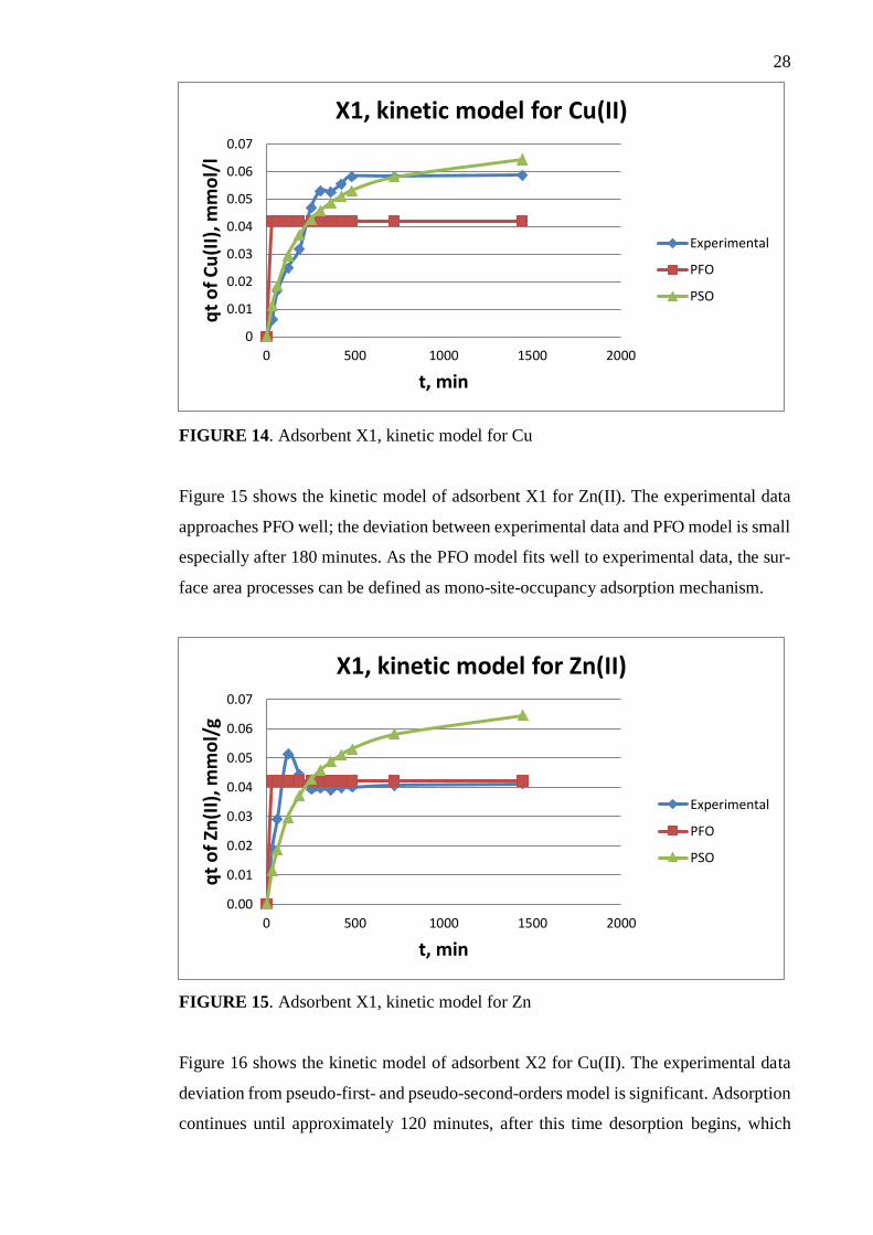
28

FIGURE 14. Adsorbent X1, kinetic model for Cu

Figure 15 shows the kinetic model of adsorbent X1 for Zn(II). The experimental data

approaches PFO well; the deviation between experimental data and PFO model is small

especially after 180 minutes. As the PFO model fits well to experimental data, the sur-

face area processes can be defined as mono-site-occupancy adsorption mechanism.

FIGURE 15. Adsorbent X1, kinetic model for Zn

Figure 16 shows the kinetic model of adsorbent X2 for Cu(II). The experimental data

deviation from pseudo-first- and pseudo-second-orders model is significant. Adsorption

continues until approximately 120 minutes, after this time desorption begins, which

0

0.01

0.02

0.03

0.04

0.05

0.06

0.07

0 500 1000 1500 2000

qt

of

Cu

(II)

, mm

ol/

l

t, min

X1, kinetic model for Cu(II)

Experimental

PFO

PSO

0.00

0.01

0.02

0.03

0.04

0.05

0.06

0.07

0 500 1000 1500 2000

qt

of

Zn(I

I), m

mo

l/g

t, min

X1, kinetic model for Zn(II)

Experimental

PFO

PSO

29

continues until approximately 480 minutes. After 440 minutes the chemical reaction is

resuming. Models PFO and PSO do not fit to the experimental data.

FIGURE 16. Adsorbent X2, kinetic model for Cu

Figure 17 shows the kinetic model of adsorbent X2 for Zn(II). The experimental data

deviation from pseudo-first and pseudo-second-orders model is significant but much

lower than in Figure 16. Adsorption continues until approximately 120 minutes, after

which the desorption begins and continues until approximately 250 minutes. After 250

minutes the adsorption is resuming with a moderate increase. PFO and PSO kinetic

models are not able to describe experimental data.

0

0.01

0.02

0.03

0.04

0.05

0.06

0.07

0 500 1000 1500 2000

qe

of

Cu

(II)

, mm

ol/

g

t, min

X2, kinetic model for Cu(II)

Experimental

PFO

PSO

30

FIGURE 17. Adsorbent X2, kinetic model for Zn

8.4 Isotherm adsorption modelling

Results from ICP analyses were taken for adsorption isotherms modelling based on

Langmuir and Freundlich isotherm models. The purpose of Langmuir and Freundlich

isotherm models is to analyse adsorbent’s specific surface. According to the Langmuir

model, adsorption occurs uniformly on the active sides of the adsorbent. The Freundlich

isotherm is an empirical model that is based on adsorption on a heterogeneous surface.

Figure 18 is shown isotherm model of adsorbent X1 for Cu(II). The experimental data

deviation is lower for Freundlich’s isotherm model compared to Langmuir’s one. Freun-

lich isotherm model describes the heterogeneous nature of adsorbent surface. It means

that surface of adsorbent has a complex structure. Where, Ce (mmol/l) is equilibrium

concentration; qe (mmol/g) is equilibrium adsorption capacity of Cu(II) (mmol) by ad-

sorbent X1 (g).

0

0.01

0.02

0.03

0.04

0.05

0.06

0.07

0 500 1000 1500 2000

qe

of

Zn(I

I), m

mo

l/g

t, min

X2, kinetic model for Zn(II)

Experimental

PFO

PSO

31

FIGURE 18. Adsorbent X1, isotherm modelling for Cu

Figure 19 is shown isotherm model of adsorbent X1 for Zn(II). The experimental data

are closer to Langmuir’s isotherm model. Therefore, it can be assumed that the adsorp-

tion process occurs uniformly on the active sides of the adsorbent. Where, Ce (mmol/l)

is equilibrium concentration; qe (mmol/g) is equilibrium adsorption capacity of Zn(II)

(mmol) by adsorbent X1 (g).

FIGURE 19. Adsorbent X1, isotherm modelling for Zn

0

0.01

0.02

0.03

0.04

0.05

0.06

0.07

0 0.5 1 1.5 2 2.5 3 3.5

Ce

of

Cu

(II)

, mm

ol/

l

qe, mmol/g

Adsorbent X1, Cu(II)

experimental

Langmuir

Fraundlich

0

0.01

0.02

0.03

0.04

0.05

0.06

0 0.5 1 1.5 2 2.5

Ce

of

Zn(I

I), m

mo

l/l

qe, mmol/g

Adsorbent X1, Zn(II)

Experimental

Langmuir

Freundlich

32

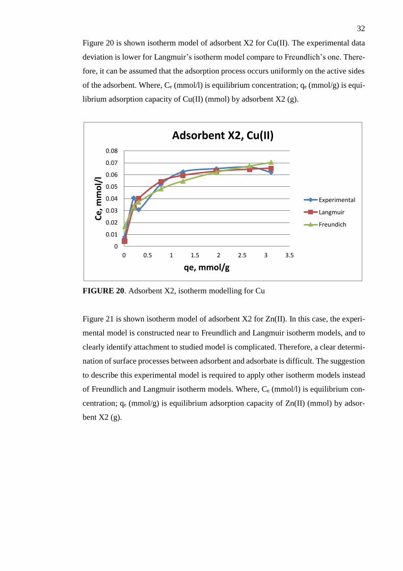
Figure 20 is shown isotherm model of adsorbent X2 for Cu(II). The experimental data

deviation is lower for Langmuir’s isotherm model compare to Freundlich’s one. There-

fore, it can be assumed that the adsorption process occurs uniformly on the active sides

of the adsorbent. Where, Ce (mmol/l) is equilibrium concentration; qe (mmol/g) is equi-

librium adsorption capacity of Cu(II) (mmol) by adsorbent X2 (g).

FIGURE 20. Adsorbent X2, isotherm modelling for Cu

Figure 21 is shown isotherm model of adsorbent X2 for Zn(II). In this case, the experi-

mental model is constructed near to Freundlich and Langmuir isotherm models, and to

clearly identify attachment to studied model is complicated. Therefore, a clear determi-

nation of surface processes between adsorbent and adsorbate is difficult. The suggestion

to describe this experimental model is required to apply other isotherm models instead

of Freundlich and Langmuir isotherm models. Where, Ce (mmol/l) is equilibrium con-

centration; qe (mmol/g) is equilibrium adsorption capacity of Zn(II) (mmol) by adsor-

bent X2 (g).

0

0.01

0.02

0.03

0.04

0.05

0.06

0.07

0.08

0 0.5 1 1.5 2 2.5 3 3.5

Ce,

mm

ol/

l

qe, mmol/g

Adsorbent X2, Cu(II)

Experimental

Langmuir

Freundich

33

FIGURE 21. Adsorbent X1, isotherm modelling for Zn

8.5 Zeta potential

In figures 22 and 23 is shown data from zeta potential experiments, the stability at dif-

ferent pH values and isoelectric point(s) of adsorbents.

Isoelectric titration graph (Fig. 22) describes adsorbent X1 at concentration 30 g/l in

water. Titration was started from 9,6 pH and completed at 1,7 pH. In a role of titrants

were HCl 1 and 0.1 M. Isoelectric points of adsorbent X1 in water are 3,3 and 9,3 pH.

Consequently, on those pH values adsorbent X1 is inactive. The highest positive zeta

potential value is 1,7mV at 1,8 pH and the highest negative zeta potential value is -3,1

mV at 6,4 pH. X1 is the most active and stable at pH value 6,4 where zeta potential

equals -3,1. Therefore, negatively charged particles of X1 at this pH value may attract

and retain positively charged particles i.e. metals ions.

0

0.01

0.02

0.03

0.04

0.05

0.06

0.07

0.08

0 0.5 1 1.5 2 2.5 3 3.5

Ce,

mm

ol/

l

qe, mmol/g

Adsorbent X2, Zn(II)

Langmuir

Experimental

Freundlich

34

FIGURE 22. Zeta potential measurements of adsorbent X1

Isoelectric titration graph (Fig. 23) describes properties of X2 at concentration 30 g/l in

water. Titration was started from 1,8 pH and completed at 9,9 pH. In a role of titrants

were NaOH 1, 0.1 and 0.01 M. Isoelectric point of adsorbent X2 in water is 5,2 pH.

Consequently, on this pH value adsorbent X2 is inactive. The highest zeta potential

value is -6,4 at 1,8 pH. X2 is the most active and stable at pH value 1,8 where zeta

potential equals -6,4. In conclusion, negatively charged particles of X2 are behaving

similar as X1.

FIGURE 23. Zeta potential measurements of adsorbent X2

35

9 CONCLUSION

The main target of this research was to study adsorption for toxic metal removal from

aqueous solution, where adsorbents X1 and X2 have shown a high removal capacity of

Zn(II) and Cu(II) from the solution. The minimum concentration with maximum ad-

sorption properties was 50 g/l for both adsorbents. The most efficient adsorption capac-

ity of adsorbent X1 was at neutral pH value and for X2 acidic pH value. In comparison

between the studied adsorbents, X2 has shown brilliant removal capacity, which equals

almost 100% in removing Zn(II) and Cu(II) from aqueous solution. Therefore, adsor-

bent X2 can be applied for further wastewater treatment experiments based on real

wastewater contaminated by Zn(II) and/or Cu(II). The results from experiments can be

used for large scale adsorption process designing by using preferably adsorbent X2.

36

BIBLIOGRAPHY

1. Isidorov V. 1997. Introduction to Chemical Eco-toxicology. Saint-Petersburg State

University, 54-58.

2. Iakovleva E. Sillanpää M. 2013. The Use of Low Cost Adsorbents for Wastewater

Purification in Mining Industries. Environmental Science and Pollution Research. Vol.

20, issue 11, 7878-7899.

3. McKay G. 1996. Use of Adsorbents for the Removal of Pollutants from

Wastewaters. CRC Press, Inc. Hong Kong, 40-43.

4. Wolkersdorfer C. 2013. From Ground Water to Mine Water. Workshop on Mine

Water Management and Remediation. Lappeenranta University of Technology, 2013.

Conference. Finland. Mikkeli, 8-11.01.2013.

5. Sharma Y. 2013. A Guide to the Economic Removal of Metals from Aqueous Solu-

tions. Wiley (Scrivener), 31-43.

6. Klaassen C. 2001. Casarett & Doull’s, Toxicology, 6th edition. The Basic Science of

Poisons. McGraw-Hill, 811-876.

7. European Commission. 2013. Urban Waste Water Directive Overview, 2013.

WWW-document.

http://ec.europa.eu/environment/water/water-urbanwaste/.

Updated: 2013. Referred: 17.04.2013.

8. European Commission, 2001. Pollutants in urban wastewater and sewage sludge.

PDF-document.

ec.europa.eu/environment/waste/sludge/pdf/sludge_pollutants.pdf.


9. Fomkin A. 2009. Nanoporous Material and Their Adsorption Properties. Institute of

Physical Chemistry and Electrochemistry, Russian Academy of Sciences, Vol. 45, is-

sue 2, 133–149.

37

10. Dabrowski A. 2001. Adsorption – from theory to practice, Advances in Colloid

and Interface Science. Faculty of Chemistry, M.Curie-Sklodowska University, Lublin,

Poland. Vol. 93, issue 1-3, 135-224.

11. Repo E. 2011. EDTA- and DTPA- Functionalized Silica Gel and Chitosan Adsor-

bents for the Removal of Heavy Metals From Aqueous Solutions. Lappeenranta Uni-

versity of Technology. Thesis.

12. Schlapbach L. 2009. Mechanisms of hydrogen storage. WWW-document.

http://www.nature.com/nature/journal/v460/n7257/fig_tab/460809a_F2.html.


13. Willis T. 2009. Sorbents – Properties, Materials and Applications. Nova Science

Publishers, Inc. New York, 52-104.

14. Chemical Systems 2013. Activated Carbon. WWW-document.

http://www.chemsystem.ru/aktivirovannyy_ugol/.


15. Treatment Solutions, Lentech 2012. Activated Carbon. WWW-document.

http://www.lenntech.com/library/adsorption/adsorption.htm.


16. Liu Grace. CO-sunny technology CO, Limited 2008. Activated Carbon. WWW-

document.

http://www.chem-hort.com/main/en_product_info.asp?id=641.


17. AquaVenture. Innovative Production Group. Zeolite 2012. WWW-document.

http://aquaventure.ru/page_154_zeolite.html.


18. Sorbead India. Activated Alumina 2013. WWW-document.

http://www.sorbeadindia.net/activated-alumina-345679.html.

38


19. AquaVenture, Innovative Production Group. Activated Carbon 2012. WWW-

document.

http://aquaventure.ru/page_153_oksid_aljuminija.html.


20. China Silica Gel Co. WWW-document.

http://www.china-silicagel.com/product/fine-pore.html.

Updated: not available. Referred: 11.03.2013.

21. Environmental Protection, Chitosan 2010. WWW-document.

http://www.eco-oos.ru/biblio/sborniki-nauchnyh-trudov/ekologicheski-ustoichivoe-

razvitie-racionalnoe-ispolzovanie-prirodnyh-resursov/62/.


22. Made-in-China.com TM. Chitosan. WWW-document.

http://cnreachem.en.made-in-china.com/productimage/dMcxIiwhMSUB-

2f0j00WMetYLBsCjrl/China-Chitosan-Nitrate.html.

Updated: not available. Referred: 11.03.2013.

23. SciVerse, ScienceDirect (Biotechnology Advances, Biosorbents) 2013. WWW-

document.

http://www.sciencedirect.com/science/article/pii/S0734975008001109.


APPENDIX 1(1).

Data from experiments

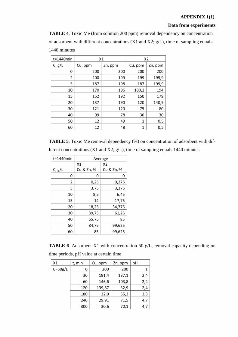
TABLE 4. Toxic Me (from solution 200 ppm) removal dependency on concentration

of adsorbent with different concentrations (X1 and X2; g/L), time of sampling equals

1440 minutes

t=1440min X1 X2

C, g/L Cu, ppm Zn, ppm Cu, ppm Zn, ppm

0 200 200 200 200

2 200 199 199 199,9

5 187 198 187 199,9

10 170 196 180,2 194

15 152 192 150 179

20 137 190 120 140,9

30 121 120 75 80

40 99 78 30 30

50 12 49 1 0,5

60 12 48 1 0,5

TABLE 5. Toxic Me removal dependency (%) on concentration of adsorbent with dif-

ferent concentrations (X1 and X2; g/L), time of sampling equals 1440 minutes

t=1440min Average

C, g/L X1 Cu & Zn, %

X2, Cu & Zn, %

0 0 0

2 0,25 0,275

5 3,75 3,275

10 8,5 6,45

15 14 17,75

20 18,25 34,775

30 39,75 61,25

40 55,75 85

50 84,75 99,625

60 85 99,625

TABLE 6. Adsorbent X1 with concentration 50 g/L, removal capacity depending on

time periods, pH value at certain time

X1 t, min Cu, ppm Zn, ppm pH

C=50g/L 0 200 200 1

30 191,4 137,1 2,4

60 146,6 103,8 2,4

120 139,87 32,9 2,4

180 32,9 55,3 3,3

240 29,91 71,5 4,7

300 30,6 70,1 4,7

APPENDIX 1(2).


360 31,8 72,3 4,9

420 22,5 69,9 5,4

480 13,9 69,1 5,4

720 13,8 67,2 5,9

1440 12,2 65,6 6,3

TABLE 7. Adsorbent X1 with concentration 50 g/L, removal capacity (%) depending

on time periods, pH value at certain time

X1 t, min Cu, % Zn, % pH

C=50g/L 0 0 0 1

30 4,3 31,45 2,4

60 26,7 48,1 2,4

120 30,065 83,55 2,4

180 83,55 72,35 3,3

240 85,045 64,25 4,7

300 84,7 64,95 4,7

360 84,1 63,85 4,9

420 88,75 65,05 5,4

480 93,05 65,45 5,4

720 93,1 66,4 5,9

1440 93,9 67,2 6,3

TABLE 8. Adsorbent X2 with concentration 50 g/L, removal capacity depending on

time periods, pH value at certain time

X2 t, min Cu, ppm Zn, ppm pH

C=50g/L 0 200 200 1

30 170,2 189,5 1,4

60 117,4 62,3 1,4

120 69,9 24,1 1,4

180 100,2 48,1 1,4

240 115,2 86,76 1,4

300 119,1 42,2 1,3

360 118,7 35,2 1,3

420 119,3 35,5 1,4

480 104,1 34,6 1,5

720 70,7 39,5 1,5

1440 1,4 0,51 1,5

TABLE 9. Adsorbent X2 with concentration 50 g/L, removal capacity (%) depending

on time periods, pH value at certain time

X2 t, min Cu, % Zn, % pH

APPENDIX 1(3).


C=50g/L 0 0 0 1

30 14,9 5,25 1,4

60 41,3 68,85 1,4

120 65,05 87,95 1,4

180 49,9 75,95 1,4

240 42,4 56,62 1,4

300 40,45 78,9 1,3

360 40,65 82,4 1,3

420 40,35 82,25 1,4

480 47,95 82,7 1,5

720 64,65 80,25 1,5

1440 99,3 99,745 1,5

TABLE 10. Adsorbent X1 with concentration 50 g/L, removal capacity of Cu depend-

ing on time

X1/Сu t, min Cu ppm CCu, mmol/l

C=50g/L 0 200 3,125000

30 180 2,812500

60 146,6 2,290625

120 120 1,875000

180 98 1,531250

240 50 0,78125

300 30,6 0,478125

360 31,8 0,496875

420 22,5 0,351563

480 13,9 0,217188

720 13,8 0,215625

1440 12,2 0,190625

TABLE 11. Modelling adsorption kinetics of X1 for Cu by non-linear kinetic modelling

of pseudo-first-order and pseudo-second-order

X1/Cu Pseudo-first-order Pseudo-second-order

qe 0,042062 qe 0,072236

Experimental kinetic data k 1 k 0,079107

t qt (mmol/g) q (mmol/g) ERRSQ q (mmol/g) ERRSQ

0 0 0 0 0 0

32 0,006250 0,042062 0,001283 0,011167121 2,42E-05

61 0,016687 0,042062 0,000644 0,018671479 3,94E-06

121 0,025000 0,042062 0,000291 0,029529326 2,05E-05

185 0,031875 0,042062 0,000104 0,037121746 2,75E-05

252 0,046875 0,042062 2,32E-05 0,042631569 1,8E-05

APPENDIX 1(4).


304 0,0529375 0,042062 0,000118 0,04584547 5,03E-05

362 0,0525625 0,042062 0,00011 0,048695898 1,5E-05

421 0,0554687 0,042062 0,00018 0,051026257 1,97E-05

482 0,0581562 0,042062 0,000259 0,052995545 2,66E-05

721 0,0581875 0,042062 0,00026 0,058127878 3,55E-09

1444 0,0586875 0,042062 0,000276 0,064428345 3,3E-05

Sum 0,003548 Sum 0,000239

TABLE 12. Adsorbent X1 with concentration 50 g/L, removal capacity of Zn depend-

ing on time

X1/Zn t, min Zn ppm CCu

C=50g/L 0 200 3,125000

30 137,1 2,142188

60 103,8 1,621875

120 32,9 0,514063

180 55,3 0,864063

240 71,5 1,117188

300 70,1 1,095313

360 72,3 1,129688

420 69,9 1,092188

480 69,1 1,079688

720 67,2 1,050000

1440 65,6 1,025000

TABLE 13. Modelling adsorption kinetics of X1 for Zn by non-linear kinetic modelling


X1/Zn Pseudo-first-order Pseudo-second-or-

der

qe 1 qe 1

Experimental kinetic data k 1 k 1

t qt (mmol/g) q (mmol/g) ERRSQ

q (mmol/g) ERRSQ

0 0 0 9,24556E-07 0 9,25E-07

32 0,018694712 0,042062 0,000546054 0,011167 5,67E-05

61 0,029100962 0,042062 0,000168001 0,018671 0,000109

121 0,051257212 0,042062 8,45427E-05 0,029529 0,000472

185 0,044257212 0,042062 4,81676E-06 0,037122 5,09E-05

252 0,039194712 0,042062 8,22421E-06 0,042632 1,18E-05

304 0,039632212 0,042062 5,9063E-06 0,045845 3,86E-05

362 0,038944712 0,042062 9,7206E-06 0,048696 9,51E-05

421 0,039694712 0,042062 5,60642E-06 0,051026 0,000128

482 0,039944712 0,042062 4,48503E-06 0,052996 0,00017

721 0,040538462 0,042062 2,32269E-06 0,058128 0,000309

1444 0,041038462 0,042062 1,04865E-06 0,064428 0,000547

APPENDIX 1(5).


Sum 0,000841653 Sum 0,00199

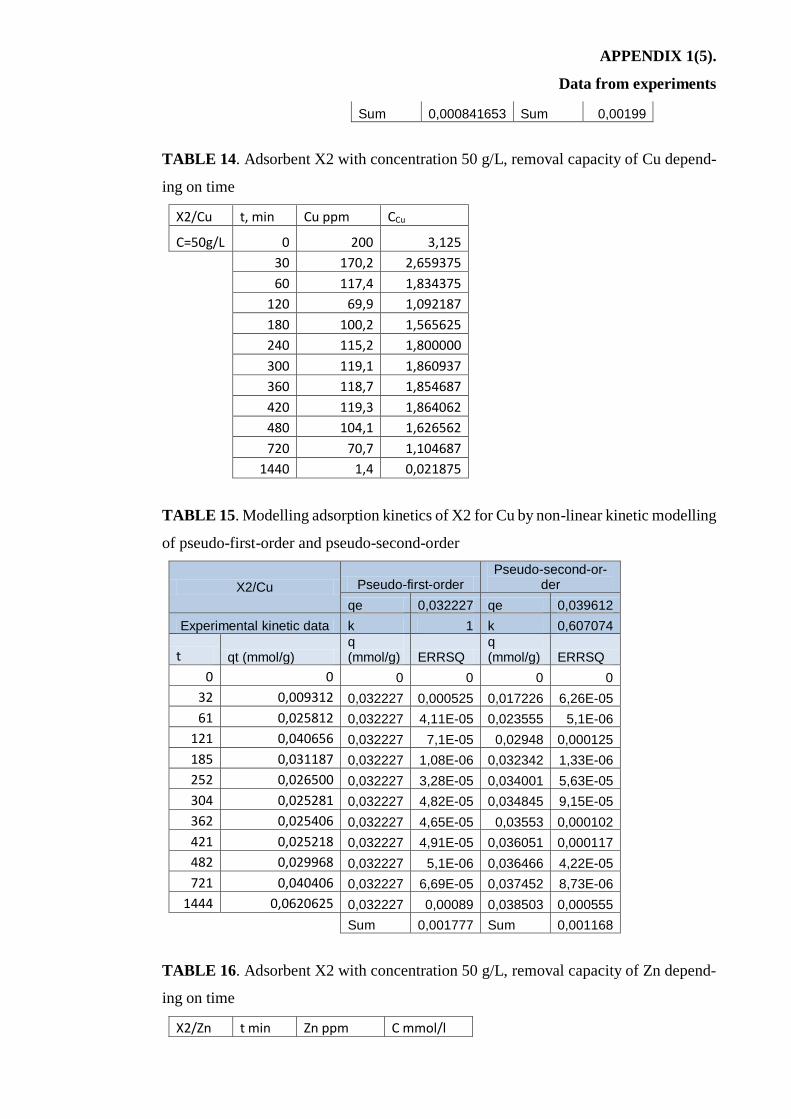
TABLE 14. Adsorbent X2 with concentration 50 g/L, removal capacity of Cu depend-

ing on time

X2/Сu t, min Cu ppm CCu

C=50g/L 0 200 3,125

30 170,2 2,659375

60 117,4 1,834375

120 69,9 1,092187

180 100,2 1,565625

240 115,2 1,800000

300 119,1 1,860937

360 118,7 1,854687

420 119,3 1,864062

480 104,1 1,626562

720 70,7 1,104687

1440 1,4 0,021875

TABLE 15. Modelling adsorption kinetics of X2 for Cu by non-linear kinetic modelling


X2/Cu Pseudo-first-order Pseudo-second-or-

der

qe 0,032227 qe 0,039612


t qt (mmol/g) q (mmol/g) ERRSQ

q (mmol/g) ERRSQ

0 0 0 0 0 0

32 0,009312 0,032227 0,000525 0,017226 6,26E-05

61 0,025812 0,032227 4,11E-05 0,023555 5,1E-06

121 0,040656 0,032227 7,1E-05 0,02948 0,000125

185 0,031187 0,032227 1,08E-06 0,032342 1,33E-06

252 0,026500 0,032227 3,28E-05 0,034001 5,63E-05

304 0,025281 0,032227 4,82E-05 0,034845 9,15E-05

362 0,025406 0,032227 4,65E-05 0,03553 0,000102

421 0,025218 0,032227 4,91E-05 0,036051 0,000117

482 0,029968 0,032227 5,1E-06 0,036466 4,22E-05

721 0,040406 0,032227 6,69E-05 0,037452 8,73E-06

1444 0,0620625 0,032227 0,00089 0,038503 0,000555

Sum 0,001777 Sum 0,001168

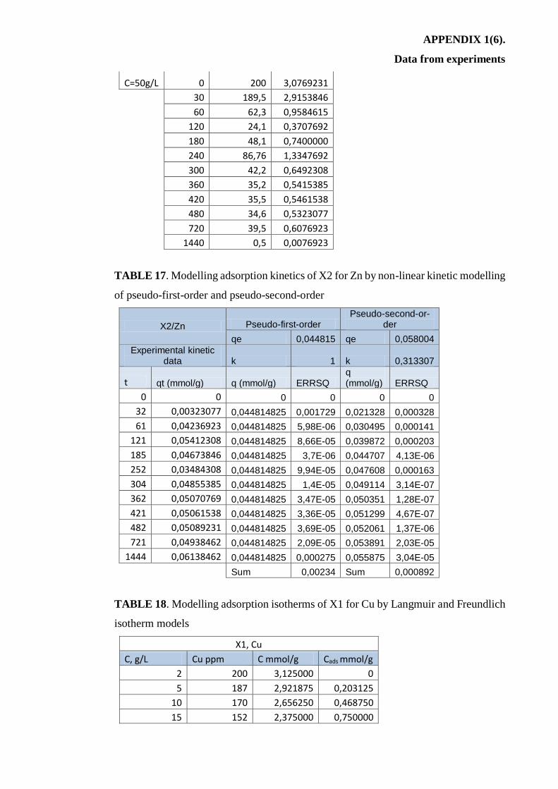
TABLE 16. Adsorbent X2 with concentration 50 g/L, removal capacity of Zn depend-

ing on time

X2/Zn t min Zn ppm C mmol/l

APPENDIX 1(6).


C=50g/L 0 200 3,0769231

30 189,5 2,9153846

60 62,3 0,9584615

120 24,1 0,3707692

180 48,1 0,7400000

240 86,76 1,3347692

300 42,2 0,6492308

360 35,2 0,5415385

420 35,5 0,5461538

480 34,6 0,5323077

720 39,5 0,6076923

1440 0,5 0,0076923

TABLE 17. Modelling adsorption kinetics of X2 for Zn by non-linear kinetic modelling


X2/Zn Pseudo-first-order Pseudo-second-or-

der

qe 0,044815 qe 0,058004


t qt (mmol/g) q (mmol/g) ERRSQ q (mmol/g) ERRSQ

0 0 0 0 0 0

32 0,00323077 0,044814825 0,001729 0,021328 0,000328

61 0,04236923 0,044814825 5,98E-06 0,030495 0,000141

121 0,05412308 0,044814825 8,66E-05 0,039872 0,000203

185 0,04673846 0,044814825 3,7E-06 0,044707 4,13E-06

252 0,03484308 0,044814825 9,94E-05 0,047608 0,000163

304 0,04855385 0,044814825 1,4E-05 0,049114 3,14E-07

362 0,05070769 0,044814825 3,47E-05 0,050351 1,28E-07

421 0,05061538 0,044814825 3,36E-05 0,051299 4,67E-07

482 0,05089231 0,044814825 3,69E-05 0,052061 1,37E-06

721 0,04938462 0,044814825 2,09E-05 0,053891 2,03E-05

1444 0,06138462 0,044814825 0,000275 0,055875 3,04E-05

Sum 0,00234 Sum 0,000892

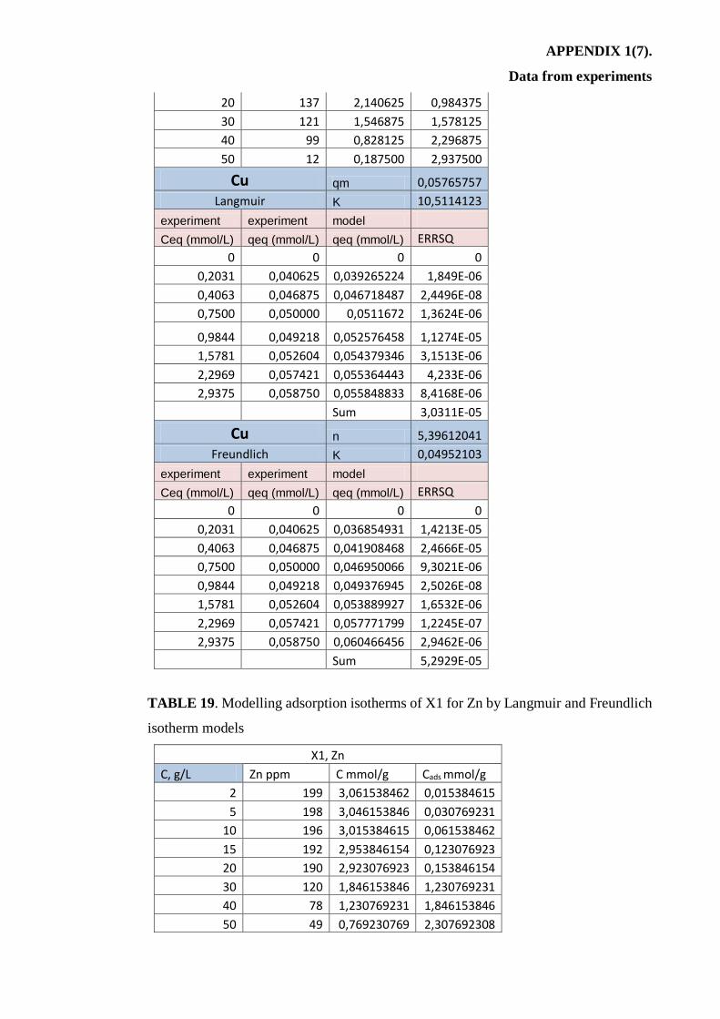
TABLE 18. Modelling adsorption isotherms of X1 for Cu by Langmuir and Freundlich

isotherm models

X1, Cu

C, g/L Cu ppm C mmol/g Cads mmol/g

2 200 3,125000 0

5 187 2,921875 0,203125

10 170 2,656250 0,468750

15 152 2,375000 0,750000

APPENDIX 1(7).


20 137 2,140625 0,984375

30 121 1,546875 1,578125

40 99 0,828125 2,296875

50 12 0,187500 2,937500

Cu qm 0,05765757

Langmuir K 10,5114123

experiment experiment model

Ceq (mmol/L) qeq (mmol/L) qeq (mmol/L) ERRSQ

0 0 0 0

0,2031 0,040625 0,039265224 1,849E-06

0,4063 0,046875 0,046718487 2,4496E-08

0,7500 0,050000 0,0511672 1,3624E-06

0,9844 0,049218 0,052576458 1,1274E-05

1,5781 0,052604 0,054379346 3,1513E-06

2,2969 0,057421 0,055364443 4,233E-06

2,9375 0,058750 0,055848833 8,4168E-06

Sum 3,0311E-05

Cu n 5,39612041

Freundlich K 0,04952103



0 0 0 0

0,2031 0,040625 0,036854931 1,4213E-05

0,4063 0,046875 0,041908468 2,4666E-05

0,7500 0,050000 0,046950066 9,3021E-06

0,9844 0,049218 0,049376945 2,5026E-08

1,5781 0,052604 0,053889927 1,6532E-06

2,2969 0,057421 0,057771799 1,2245E-07

2,9375 0,058750 0,060466456 2,9462E-06

Sum 5,2929E-05

TABLE 19. Modelling adsorption isotherms of X1 for Zn by Langmuir and Freundlich

isotherm models

X1, Zn

C, g/L Zn ppm C mmol/g Cads mmol/g

2 199 3,061538462 0,015384615

5 198 3,046153846 0,030769231

10 196 3,015384615 0,061538462

15 192 2,953846154 0,123076923

20 190 2,923076923 0,153846154

30 120 1,846153846 1,230769231

40 78 1,230769231 1,846153846

50 49 0,769230769 2,307692308

APPENDIX 1(8).


Zn qm 0,066314578




0,015384615 0,007692308 0,001134083 4,30103E-05

0,030769231 0,006153846 0,002230029 1,53963E-05

0,061538462 0,006153846 0,004314954 3,38153E-06

0,123076923 0,008205128 0,008102683 1,04951E-08

0,153846154 0,007692308 0,009828139 4,56178E-06

1,230769231 0,041025641 0,038590269 5,93104E-06

1,846153846 0,046153846 0,044838909 1,72906E-06

2,307692308 0,046153846 0,047944211 3,20541E-06

Sum 7,7226E-05

Zn n 0,863496227




0,015384615 0,007692308 0,007692303 2,47557E-17

0,030769231 0,006153846 0,025978253 0,000393007

0,061538462 0,006153846 0,029539036 0,000546867

0,123076923 0,008205128 0,033587888 0,000644284

0,153846154 0,007692308 0,035005952 0,000746035

1,230769231 0,041025641 0,051463702 0,000108953

1,846153846 0,046153846 0,055479682 8,69712E-05

2,307692308 0,046153846 0,057822007 0,000136146

Sum 0,002662264

TABLE 20. Modelling adsorption isotherms of X2 for Cu by Langmuir and Freundlich

isotherm models

X2, Cu

C/g/L Cu ppm C mmol/g Cads mmol/g

2 199 3,109375 0,015625

5 187 2,921875 0,203125

10 180,2 2,815625 0,309375

15 150 2,34375 0,78125

20 120 1,875 1,25

30 75 1,171875 1,953125

40 30 0,46875 2,65625

50 1 0,015625 3,109375

Cu qm 0,070316418


experiment experiment model Ceq (mmol/L)

qeq (mmol/L)

qeq (mmol/L) ERRSQ

APPENDIX 1(9).


0,015625 0,007812 0,004454116 1,12787E-05

0,203125 0,040625 0,032897352 5,97165E-05

0,309375 0,030937 0,040254186 8,68006E-05

0,78125 0,052083 0,054267517 4,77066E-06

1,25 0,062500 0,059346988 9,94149E-06

1,953125 0,065104 0,062878253 4,95469E-06

2,65625 0,066406 0,064689623 2,94681E-06

3,109375 0,062187 0,065452893 1,06628E-05

Sum 0,000191072

Cu n 3,656159706



qeq (mmol/L)

qeq (mmol/L) ERRSQ

0,015625 0,007812 0,016533762 7,60604E-05

0,203125 0,040625 0,033346286 5,29797E-05

0,309375 0,030937 0,037413119 4,19336E-05

0,78125 0,052083 0,048201296 1,50702E-05

1,25 0,062500 0,054813532 5,90818E-05

1,953125 0,065104 0,061929803 1,00766E-05

2,65625 0,066406 0,06736341 9,16155E-07

3,109375 0,062187 0,070328824 6,62812E-05

Sum 0,0003224

TABLE 21. Modelling adsorption isotherms of X2 for Zn by Langmuir and Freundlich

isotherm models

X2, Zn

C/g/L Zn ppm C mmol/g Cads mmol/g

2 199,9 3,075385 0,001538

5 199,9 3,075385 0,001538

10 194 2,984615 0,092308

15 179 2,753846 0,323077

20 140,9 2,167692 0,909231

30 80 1,230769 1,846154

40 30 0,461538 2,615385

50 0,5 0,007692 3,069231

Zn qm 0,082206

Langmuir K 1,289027


qeq (mmol/L)

qeq (mmol/L) ERRSQ

0,001538 0,000769 0,000163 3,68E-07

0,001538 0,000308 0,000163 2,1E-08

0,092308 0,009231 0,008741 2,4E-07

APPENDIX 1(10).


0,323077 0,021538 0,024170 6,92E-06

0,909231 0,045462 0,044358 1,22E-06

1,846154 0,061538 0,057883 1,34E-05

2,615385 0,065385 0,063400 3,94E-06

3,069231 0,061385 0,065620 1,79E-05

Sum 4,4E-05

Zn n 2,205087



qeq (mmol/L)

qeq (mmol/L) ERRSQ

0,001538 0,000769 0,002198 2,04E-06

0,001538 0,000308 0,002198 3,57E-06

0,092308 0,009231 0,014075 2,35E-05

0,323077 0,021538 0,024842 1,09E-05

0,909231 0,045462 0,039717 3,3E-05

1,846154 0,061538 0,054760 4,59E-05

2,615385 0,065385 0,064131 1,57E-06

3,069231 0,061385 0,068957 5,73E-05

Sum 0,000178

APPENDIX 2(1).

Figures

FIGURE 24. Scales Sartorius model SPA225D

FIGURE 25. Cylindrical plastic tubes 50 ml with caps

APPENDIX 2(2).

Figures

FIGURE 26. Solution of Cu((II) Cu(NO3)2*3H2O, m=3,781 g) and Zn((II)

ZnSO4*7H2O, m=4,415) mixed in water with the addition of HNO3, right 1000 ml flask

and 500 ml cylinder have 1000 ppm of those studied Me, left 2000 ml flask was made

in accordance to the concentration of studied 200 ppm

FIGURE 27. From the left side is heating plate model IKA C-MAG HS7 with a regu-

lated magnet field for mixing solutions, on the right side pH meter model WTW pH

340i

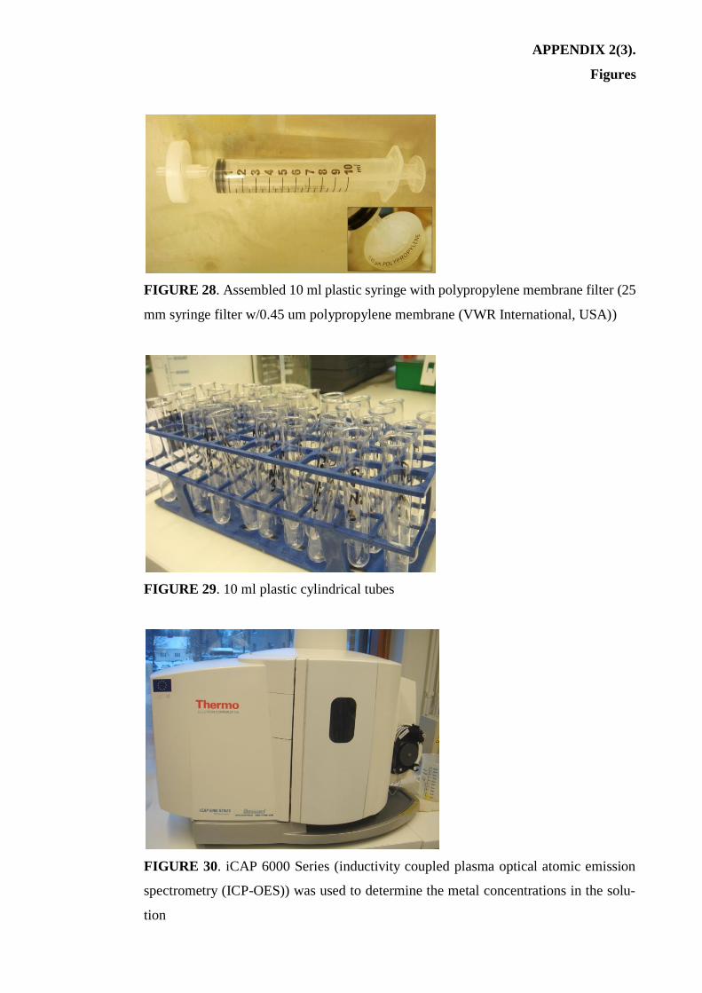
APPENDIX 2(3).

Figures

FIGURE 28. Assembled 10 ml plastic syringe with polypropylene membrane filter (25

mm syringe filter w/0.45 um polypropylene membrane (VWR International, USA))

FIGURE 29. 10 ml plastic cylindrical tubes

FIGURE 30. iCAP 6000 Series (inductivity coupled plasma optical atomic emission

spectrometry (ICP-OES)) was used to determine the metal concentrations in the solu-

tion

APPENDIX 2(4).

Figures

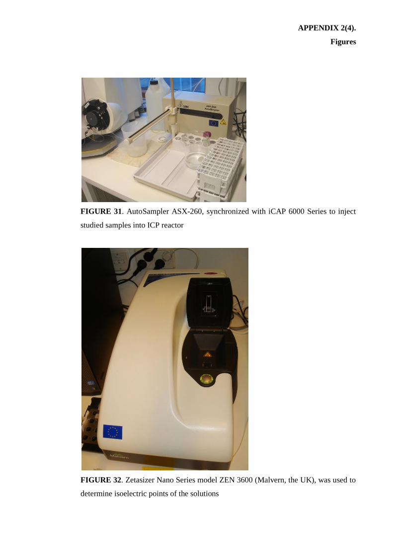
FIGURE 31. AutoSampler ASX-260, synchronized with iCAP 6000 Series to inject

studied samples into ICP reactor

FIGURE 32. Zetasizer Nano Series model ZEN 3600 (Malvern, the UK), was used to

determine isoelectric points of the solutions

APPENDIX 2(5).

Figures

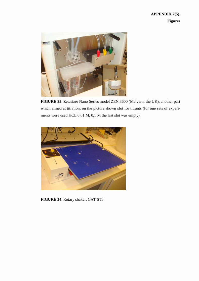
FIGURE 33. Zetasizer Nano Series model ZEN 3600 (Malvern, the UK), another part

which aimed at titration, on the picture shown slot for titrants (for one sets of experi-

ments were used HCL 0,01 M, 0,1 M the last slot was empty)

FIGURE 34. Rotary shaker, CAT ST5

eduard musin (a9838) t879sn - theseus.fi

Documents