ecs 315: probability and random processes 2015/1 …...so, xis a binomial rv. problem 3. arrivals of...

ECS 315: Probability and Random Processes 2015/1

HW Solution 7 — Due: Oct 28, 9:19 AM (in tutorial session)Lecturer: Prapun Suksompong, Ph.D.

Instructions

(a) ONE part of a question will be graded (5 pt). Of course, you do not know which partwill be selected; so you should work on all of them.

(b) It is important that you try to solve all problems. (5 pt)The extra questions at the end are optional.

(c) Late submission will be heavily penalized.

Problem 1. [F2013/1] For each of the following random variables, find P [1 < X ≤ 2].

(a) X ∼ Binomial(3, 1/3)

(b) X ∼ Poisson(3)

Solution :

(a) Because X ∼ Binomial(3, 1/3), we know that X can only take the values 0, 1, 2, 3.Only the value 2 satisfies the condition given. Therefore, P [1 < X ≤ 2] = P [X = 2] =pX(2). Recall that the pmf for the binomial random variable is

pX (x) =

(n

x

)px(1− p)n−x

for x = 0, 1, 2, 3, . . . , n. Here, it is given that n = 3 and p = 1/3. Therefore,

pX(2) =

(3

2

)(1

3

)2(1− 1

3

)3−2

= 3× 1

9× 2

3=

2

9.

(b) Because X ∼ Poisson(3), we know that X can take the values 0, 1, 2, 3, . . . . As in theprevious part, only the value 2 satisfies the condition given. Therefore, P [1 < X ≤ 2] =P [X = 2] = pX(2). Recall that the pmf for the Poisson random variable is

pX (x) = e−ααx

x!

7-1

ECS 315HW Solution 7 — Due: Oct 28, 9:19 AM (in tutorial session) 2015/1

2

-1

0.064

1 0 2 4 3

0.352

0.784

1.000

x

Figure 7.1: CDF of X for Problem 2

for x = 0, 1, 2, 3, . . .. Here, it is given that α = 3. Therefore,

pX(2) = e−332

2!=

9

2e−3 ≈ 0.2240 .

Problem 2. [M2011/1] The cdf of a random variable X is plotted in Figure 7.1.

(a) Find the pmf pX(x).

(b) Find the family to which X belongs. (Uniform, Bernoulli, Binomial, Geometric, Pois-son, etc.)

Solution :

(a) For discrete random variable, P [X = x] is the jump size at x on the cdf plot. In thisproblem, there are four jumps at 0, 1, 2, 3.

• P [X = 0] = the jump size at 0 = 0.064 = 641000

= (4/10)3 = (2/5)3.

• P [X = 1] = the jump size at 1 = 0.352− 0.064 = 0.288.

• P [X = 2] = the jump size at 2 = 0.784− 0.352 = 0.432.

• P [X = 3] = the jump size at 3 = 1− 0.784 = 0.216 = (6/10)3.

7-2


In conclusion,

pX (x) =

0.064, x = 0,0.288, x = 1,0.432, x = 2,0.216, x = 3,0, otherwise.

(b) Among all the pmf that we discussed in class, only one can have support = {0, 1, 2, 3}with unequal probabilities. This is the binomial pmf. To check that it really isBinomial, recall that the pmf for binomial X is given by pX(x) =

(nx

)px(1 − p)(n−x)

for x = 0, 1, 2, . . . , n. Here, n = 3. Furthermore, observe that pX(0) = (1 − p)n. Bycomparing pX(0) with what we had in part (a), we have 1− p = 2/5 or p = 3/5. Forx = 1, 2, 3, plugging in p = 3/5 and n = 3 in to pX(x) =

(nx

)px(1 − p)(n−x) gives the

same values as what we had in part (a). So, X is a binomial RV.

Problem 3. Arrivals of customers at the local supermarket are modeled by a Poisson processwith a rate of λ = 2 customers per minute. Let M be the number of customers arrivingbetween 9:00 and 9:05. What is the probability that M < 2?

Solution : Here, we are given that M ∼ P(α) where α = λT = 2× 5 = 10. Recall that,for M ∼ P(α), we have

P [M = m] =

{e−α α

m

m!, m ∈ {0, 1, 2, 3, . . .}

0, otherwise

Therefore,

P [M < 2] = P [M = 0] + P [M = 1] = e−αα0

0!+ e−α

α1

1!= e−α (1 + α) = e−10 (1 + 10) = 11e−10 ≈ 5× 10−4.

Problem 4. When n is large, binomial distribution Binomial(n, p) becomes difficult tocompute directly because of the need to calculate factorial terms. In this question, we willconsider an approximation when the value of p is close to 0. In such case, the binomial can beapproximated1 by the Poisson distribution with parameter α = np. For this approximationto work, we will see in this exercise that n does not have to be very large and p does notneed to be very small.

1More specifically, suppose Xn has a binomial distribution with parameters n and pn. If pn → 0 andnpn → α as n→∞, then

P [Xn = k]→ e−ααk

k!.

7-3


(a) Let X ∼ Binomial(12, 1/36). (For example, roll two dice 12 times and let X be thenumber of times a double 6 appears.) Evaluate pX(x) for x = 0, 1, 2.

(b) Compare your answers part (a) with its Poisson approximation.

(c) Compare MATLAB plots of pX(x) in part (a) and the pmf of P(np).

Solution :

(a) For Binomial(n, p) random variable,

pX(x) =

{ (nx

)px(1− p)n−x, x ∈ {0, 1, 2, . . . , n},

0, otherwise.

Here, we are given that n = 12 and p = 136

. Plugging in x = 0, 1, 2, we get

0.7132, 0.2445, 0.0384 , respectively

(b) A Poisson random variable with parameter α = np can approximate a Binomial(n, p)random variable when n is large and p is small. Here, with n = 12 and p = 1

36, we

have α = 12× 136

= 13. The Poisson pmf at x = 0, 1, 2 is given by e−α α

x

x!= e−1/3 (1/3)

x

x!.

Plugging in x = 0, 1, 2 gives 0.7165, 0.2388, 0.0398 , respectively.

(c) See Figure 7.2. Note how close they are!

0 1 2 3 4 5 6 7 80

0.1

0.2

0.3

0.4

0.5

0.6

0.7

0.8

x

Binomial pmfPoisson pmf

Figure 7.2: Poisson Approximation

7-4


Problem 5. You go to a party with 500 guests. What is the probability that exactly oneother guest has the same birthday as you? Calculate this exactly and also approximately byusing the Poisson pmf. (For simplicity, exclude birthdays on February 29.) [Bertsekas andTsitsiklis, 2008, Q2.2.2]

Solution : Let N be the number of guests that has the same birthday as you. We maythink of the comparison of your birthday with each of the guests as a Bernoulli trial. Here,there are 500 guests and therefore we are considering n = 500 trials. For each trial, the(success) probability that you have the same birthday as the corresponding guest is p = 1

365.

Then, this N ∼ Binomial(n, p).

(a) Binomial: P [N = 1] = np1(1− p)n−1 ≈ 0.348.

(b) Poisson: P [N = 1] = e−np (np)1

1!≈ 0.348.

7-5


Extra Questions

Here are some optional questions for those who want more practice.

Problem 6. A sample of a radioactive material emits particles at a rate of 0.7 per sec-ond. Assuming that these are emitted in accordance with a Poisson distribution, find theprobability that in one second

(a) exactly one is emitted,

(b) more than three are emitted,

(c) between one and four (inclusive) are emitted

[Applebaum, 2008, Q5.27].

Solution : Let X be the number or particles emitted during the one second underconsideration. Then X ∼ P(α) where α = λT = 0.7× 1 = 0.7.

(a) P [X = 1] = e−α α1

1!= αe−α = 0.7e−0.7 ≈ 0.3477.

(b) P [X > 3] = 1− P [X ≤ 3] = 1−3∑

k=0

e−0.7 0.7k

k!≈ 0.0058.

(c) P [1 ≤ X ≤ 4] =4∑

k=1

e−0.7 0.7k

k!≈ 0.5026.

Problem 7 (M2011/1). You are given an unfair coin with probability of obtaining a headequal to 1/3, 000, 000, 000. You toss this coin 6,000,000,000 times. Let A be the event thatyou get “tails for all the tosses”. Let B be the event that you get “heads for all the tosses”.

(a) Approximate P (A).

(b) Approximate P (A ∪B).

Solution : Let N be the number of heads among the n tosses. Then, N ∼ B(n, p). Here, wehave small p = 1/3 × 109 and large n = 6 × 109. So, we can apply Poisson approximation.In other words, B(n, p) is well-approximated by P(α) where α = np = 2.

(a) P (A) = P [N = 0] = e−220

0!= 1

e2≈ 0.1353.

(b) P (A∪B) = P [N = 0]+P [N = n] = e−2 20

0!+e−2 26×109

(6×109)!. The second term is extremely

small compared to the first one. Hence, P (A∪B) is approximately the same as P (A).

7-6


HW Solution 8 — Due: Nov 4, 9:19 AM (in tutorial session)Lecturer: Prapun Suksompong, Ph.D.

Instructions



(c) Late submission will be heavily penalized.

Problem 1. Consider a random variable X whose pmf is

pX (x) =

1/2, x = −1,1/4, x = 0, 1,0, otherwise.

Let Y = X2.

(a) Find EX.

(b) Find E [X2].

(c) Find VarX.

(d) Find σX .

(e) Find pY (y).

(f) Find EY .

(g) Find E [Y 2].

Solution :

(a) EX =∑x

xpX (x) = (−1)× 12

+ (0)× 14

+ (1)× 14

= −12

+ 14

= −1

4.

8-1

ECS 315 HW Solution 8 — Due: Nov 4, 9:19 AM (in tutorial session) 2015/1

(b) E [X2] =∑x

x2pX (x) = (−1)2 × 12

+ (0)2 × 14

+ (1)2 × 14

= 12

+ 14

=3

4.

(c) VarX = E [X2]− (EX)2 = 34−(−1

4

)2= 3

4− 1

16=

11

16.

(d) σX =√

VarX =

√11

4.

(e) First, we build a table to see which values y of Y are possible from the values x of X:

x pX(x) y-1 1/2 (−1)2 = 10 1/4 (0)2 = 01 1/4 (1)2 = 1

Therefore, the random variable Y can takes two values: 0 and 1. pY (0) = pX(0) = 1/4.pY (1) = pX(−1) + pX(1) = 1/2 + 1/4 = 3/4. Therefore,

pY (y) =

1/4, y = 0,3/4, y = 1,0, otherwise.

(f) EY =∑y

ypY (y) = (0) × 14

+ (1) × 34

=3

4. Alternatively, because Y = X2, we

automatically have E [Y ] = E [X2]. Therefore, we can simply use the answer from part(b).

(g) E [Y 2] =∑y

y2pY (y) = (0)2 × 14

+ (1)2 × 34

=3

4. Alternatively,

E[Y 2]

= E[X4]

=∑x

x4pX (x) = (−1)4 × 1

2+ (0)4 × 1

4+ (1)4 × 1

4=

1

2+

1

4=

3

4.

Problem 2. For each of the following random variables, find EX and σX .

(a) X ∼ Binomial(3, 1/3)

(b) X ∼ Poisson(3)

Solution :

8-2


(a) From the lecture notes, we know that when X ∼ Binomial(n, p), we have EX = npand VarX = p(1− p). Here, n = 3 and p = 1/3. Therefore, EX = 3× 1

3= 1 . Also,

because VarX = 13

(1− 1

3

)= 2

9, we have σX =

√VarX =

√2

3.

(b) From the lecture notes, we know that when X ∼ Poisson(α), we have EX = α andVarX = α. Here, α = 3. Therefore, EX = 3 . Also, because VarX = 3, we have

σX =√

3 .

Problem 3. Suppose X is a uniform discrete random variable on {−3,−2,−1, 0, 1, 2, 3, 4}.Find

(a) EX

(b) E [X2]

(c) VarX

(d) σX

Solution : All of the calculations in this question are simply plugging in numbers intoappropriate formulas.

(a) EX = 0.5

(b) E [X2] = 5.5

(c) VarX = 5.25

(d) σX = 2.2913

Alternatively, we can find a formula for the general case of uniform random variable Xon the sets of integers from a to b. Note that there are n = b− a+ 1 values that the randomvariable can take. Hence, all of them has probability 1

n.

(a) EX =∑b

k=a k1n

= 1n

∑bk=a k = 1

n× n(a+b)

2= a+b

2.

8-3

Prapun

Prapun

Prapun

Prapun


(b) First, note that

b∑i=a

k (k − 1) =b∑

k=a

k (k − 1)

((k + 1)− (k − 2)

3

)

=1

3

(b∑

k=a

(k + 1) k (k − 1)−b∑

k=a

k (k − 1) (k − 2)

)=

1

3((b+ 1) b (b− 1)− a (a− 1) (a− 2))

where the last equality comes from the fact that there are many terms in the first sumthat is repeated in the second sum and hence many cancellations.

Now,b∑

k=a

k2 =b∑

k=a

(k (k − 1) + k) =b∑

k=a

k (k − 1) +b∑

k=a

k

=1

3((b+ 1) b (b− 1)− a (a− 1) (a− 2)) +

n (a+ b)

2

Therefore,

b∑k=a

k21

n=

1

3n((b+ 1) b (b− 1)− a (a− 1) (a− 2)) +

a+ b

2

=1

3a2 − 1

6a+

1

3ab+

1

6b+

1

3b2

(c) VarX = E [X2]− (EX)2 = 112

(b− a) (b− a+ 2) = 112

(n− 1)(n+ 1) = n2−112

.

(d) σX =√

VarX =√

n2−112

.

Problem 4. (Expectation + pmf + Gambling + Effect of miscalculation of probability) Inthe eighteenth century, a famous French mathematician Jean Le Rond d’Alembert, authorof several works on probability, analyzed the toss of two coins. He reasoned that becausethis experiment has THREE outcomes, (the number of heads that turns up in those twotosses can be 0, 1, or 2), the chances of each must be 1 in 3. In other words, if we let N bethe number of heads that shows up, Alembert would say that

pN(n) = 1/3 for N = 0, 1, 2. (8.1)

[Mlodinow, 2008, p 50–51]

8-4


We know that Alembert’s conclusion was wrong. His three outcomes are not equallylikely and hence classical probability formula can not be applied directly. The key is torealize that there are FOUR outcomes which are equally likely. We should not consider 0, 1,or 2 heads as the possible outcomes. There are in fact four equally likely outcomes: (heads,heads), (heads, tails), (tails, heads), and (tails, tails). These are the 4 possibilities that makeup the sample space. The actual pmf for N is

pN(n) =

1/4, n = 0, 2,1/2 n = 1,0 otherwise.

Suppose you travel back in time and meet Alembert. You could make the following betwith Alembert to gain some easy money. The bet is that if the result of a toss of two coinscontains exactly one head, then he would pay you $150. Otherwise, you would pay him $100.

Let R be Alembert’s profit from this bet and Y be the your profit from this bet.

(a) Then, R = −150 if you win and R = +100 otherwise. Use Alembert’s miscalculatedprobabilities from (8.1) to determine the pmf of R (from Alembert’s belief).

(b) Use Alembert’s miscalculated probabilities from (8.1) (or the corresponding (miscalcu-lated) pmf found in part (a)) to calculate ER, the expected profit for Alembert.

Remark: You should find that ER > 0 and hence Alembert will be quite happy toaccept your bet.

(c) Use the actual probabilities, to determine the pmf of R.

(d) Use the actual pmf, to determine ER.

Remark: You should find that ER < 0 and hence Alembert should not accept yourbet if he calculates the probabilities correctly.

(e) Note that Y = +150 if you win and Y = −100 otherwise. Use the actual probabilitiesto determine the pmf of Y .

(f) Use the actual probabilities, to determine EY .

Remark: You should find that EY > 0. This is the amount of money that you expectto gain each time that you play with Alembert. Of course, Alembert, who still believesthat his calculation is correct, will ask you to play this bet again and again believingthat he will make profit in the long run.

By miscalculating probabilities, one can make wrong decisions (and lose a lot of money)!

Solution :

8-5


(a) P [R = −150] = P [N = 1] and P [R = +100] = P [N 6= 1] = P [N = 0] + P [N = 2].So,

pR(r) =

pN(1), r = −150,pN(0) + pN(2), r = +100,0, otherwise.

Using Alembert’s miscalculated pmf,

pR(r) =

1/3, r = −150,2/3, r = +100,0, otherwise

(b) From pR(r) in part (a), we have ER =∑

r pR(r) = 13×(−150)+ 2

3×100 =

50

3≈ 16.67

(c) Again,

pR(r) =

pN(1), r = −150,pN(0) + pN(2), r = +100,0, otherwise

Using the actual pmf,

pR(r) =

12, r = −150,

14

+ 14, r = +100,

0, otherwise=

{12, r = −150 or + 100,

0, otherwise.

(d) From pR(r) in part (c), we have ER =∑

r pR(r) = 12× (−150) + 1

2× 100 = −25 .

(e) Observe that Y = −R. Hence, using the answer from part (d), we have

pR(r) =

{12, r = +150 or − 100,

0, otherwise.

(f) Observe that Y = −R. Hence, EY = −ER. Using the actual probabilities, ER = −25from part (d). Hence, EY = +25 .

Extra Questions


8-6


Problem 5. A random variables X has support containing only two numbers. Its expectedvalue is EX = 5. Its variance is VarX = 3. Give an example of the pmf of such a randomvariable.

Solution : We first find σX =√

VarX =√

3. Recall that this is the average deviationfrom the mean. Because X takes only two values, we can make them at exactly ±

√3 from

the mean; that isx1 = 5−

√3 and x2 = 5 +

√3.

In which case, we automatically have EX = 5 and VarX = 3. Hence, one example of suchpmf is

pX(x) =

{12, x = 5±

√3

0, otherwise

We can also try to find a general formula for x1 and x2. If we let p = P [X = x2], thenq = 1 − p = P [X = x1]. Given p, the values of x1 and x2 must satisfy two conditions:EX = m and VarX = σ2. (In our case, m = 5 and σ2 = 3.) From EX = m, we must have

x1q + x2p = m; (8.2)

that isx1 =

m

q− x2

p

q.

From VarX = σ2, we have E [X2] = VarX + EX2 = σ2 +m2 and hence we must have

x21q + x22p = σ2 +m2. (8.3)

Substituting x1 from (8.2) into (8.3), we have

x22p− 2x2mp+(pm2 − qσ2

)= 0

whose solutions are

x2 =2mp±

√4m2p2 − 4p (pm2 − qσ2)

2p=

2mp± 2σ√pq

2p= m± σ

√q

p.

Using (8.2), we have

x1 =m

q−(m± σ

√q

p

)p

q= m∓ σ

√p

q.

Therefore, for any given p, there are two pmfs:

pX(x) =

1− p, x = m− σ

√p

1−p

p, x = m+ σ√

1−pp

0, otherwise,

8-7


or

pX(x) =

1− p, x = m+ σ

√p

1−p

p, x = m− σ√

1−pp

0, otherwise.

Problem 6. For each of the following families of random variable X, find the value(s) of xwhich maximize pX(x). (This can be interpreted as the “mode” of X.)

(a) P(α)

(b) Binomial(n, p)

(c) G0(β)

(d) G1(β)

Remark [Y&G, p. 66]:

• For statisticians, the mode is the most common number in the collection of observa-tions. There are as many or more numbers with that value than any other value. Ifthere are two or more numbers with this property, the collection of observations iscalled multimodal. In probability theory, a mode of random variable X is a numberxmode satisfying

pX (xmode) ≥ pX(x) for all x.

• For statisticians, the median is a number in the middle of the set of numbers, in thesense that an equal number of members of the set are below the median and above themedian. In probability theory, a median, Xmedian, of random variable X is a numberthat satisfies

P [X < Xmedian] = P [X > Xmedian] .

• Neither the mode nor the median of a random variable X need be unique. A randomvariable can have several modes or medians.

Solution : We first note that when α > 0, p ∈ (0, 1), n ∈ N, and β ∈ (0, 1), the abovepmf’s will be strictly positive for some values of x. Hence, we can discard those x at whichpX(x) = 0. The remaining points are all integers. To compare them, we will evaluate pX(i+1)

pX(i).

(a) For Poisson pmf, we have

pX (i+ 1)

pX (i)=

e−ααi+1

(i+1)!

e−ααi

i!

=α

i+ 1.

Notice that

8-8


• pX(i+1)pX(i)

> 1 if and only if i < α− 1.

• pX(i+1)pX(i)

= 1 if and only if i = α− 1.

• pX(i+1)pX(i)

< 1 if and only if i > α− 1.

Let τ = α − 1. This implies that τ is the place where things change. Moving from ito i + 1, the probability strictly increases if i < τ . When i > τ , the next probabilityvalue (at i+ 1) will decrease.

(i) Suppose α ∈ (0, 1), then α − 1 < 0 and hence i > α − 1 for all i. (Note that iare are nonnegative integers.) This implies that the pmf is a strictly decreasingfunction and hence the maximum occurs at the first i which is i = 0.

(ii) Suppose α ∈ N. Then, the pmf will be strictly increasing until we reaches i = α−1.At which point, the next probability value is the same. Then, as we furtherincrease i, the pmf is strictly decreasing. Therefore, the maximum occurs at α−1and α.

(iii) Suppose α /∈ N and α ≥ 1. Then we will have have any i = α − 1. Thepmf will be strictly increasing where the last increase is from i = bα − 1c toi + 1 = bα − 1c + 1 = bαc. After this, the pmf is strictly decreasing. Hence, themaximum occurs at bαc.

To summarize,

arg maxx

pX (x) =

0, α ∈ (0, 1),α− 1 and α, α is an integer,bαc, α > 1 is not an integer.

(b) For binomial pmf, we have

pX (i+ 1)

pX (i)=

n!(i+1)!(n−i−1)!

pi+1(1− p)n−i−1

n!i!(n−i)!p

i(1− p)n−i=

(n− i) p(i+ 1) (1− p)

.

Notice that

• pX(i+1)pX(i)

> 1 if and only if i < np− 1 + p = (n+ 1)p− 1.

• pX(i+1)pX(i)

= 1 if and only if i = (n+ 1)p− 1.

• pX(i+1)pX(i)

< 1 if and only if i > (n+ 1)p− 1.

8-9


Let τ = (n+1)p−1. This implies that τ is the place where things change. Moving fromi to i+ 1, the probability strictly increases if i < τ . When i > τ , the next probabilityvalue (at i+ 1) will decrease.

(i) Suppose (n+1)p is an integer. The pmf will strictly increase as a function of i, andthen stays at the same value at i = τ = (n+1)p−1 and i+1 = (n+1)p−1+1 =(n+ 1)p. Then, it will strictly decrease. So, the maximum occurs at (n+ 1)p− 1and (n+ 1)p.

(ii) Suppose (n + 1)p is not an integer. Then, there will not be any i that is = τ .Therefore, we only have the pmf strictly increases where the last increase occurswhen we goes from i = bτc to i + 1 = bτc + 1. After this, the probabilityis strictly decreasing. Hence, the maximum is unique and occur at bτc + 1 =b(n+ 1)p− 1c+ 1 = b(n+ 1)pc.

To summarize,

arg maxx

pX (x) =

{(n+ 1)p− 1 and (n+ 1)p, (n+ 1)p is an integer,b(n+ 1)pc, (n+ 1)p is not an integer.

(c) pX(i+1)pX(i)

= β < 1. Hence, pX(i) is strictly decreasing. The maximum occurs at the

smallest value of i which is 0 .

(d) pX(i+1)pX(i)

= β < 1. Hence, pX(i) is strictly decreasing. The maximum occurs at the

smallest value of i which is 1 .

Problem 7. An article in Information Security Technical Report [“Malicious Software—Past, Present and Future” (2004, Vol. 9, pp. 618)] provided the data (shown in Figure 8.1)on the top ten malicious software instances for 2002. The clear leader in the number ofregistered incidences for the year 2002 was the Internet worm “Klez”. This virus was firstdetected on 26 October 2001, and it has held the top spot among malicious software for thelongest period in the history of virology.

Suppose that 20 malicious software instances are reported. Assume that the malicioussources can be assumed to be independent.

(a) What is the probability that at least one instance is “Klez”?

(b) What is the probability that three or more instances are “Klez”?

(c) What are the expected value and standard deviation of the number of “Klez” instancesamong the 20 reported?

8-10


3-6 BINOMIAL DISTRIBUTION 85

and they can be considered to be independent for mutation.Determine the following probabilities. The binomial table inAppendix A can help.(a) No samples are mutated.(b) At most one sample is mutated.(c) More than half the samples are mutated.

3-89. An article in Information Security Technical Report[“Malicious Software—Past, Present and Future” (2004, Vol. 9,pp. 6–18)] provided the following data on the top ten mali-cious software instances for 2002. The clear leader in the num-ber of registered incidences for the year 2002 was the Internetworm “Klez,” and it is still one of the most widespread threats.This virus was first detected on 26 October 2001, and it hasheld the top spot among malicious software for the longest period in the history of virology.

Place Name % Instances

1 I-Worm.Klez 61.22%

2 I-Worm.Lentin 20.52%

3 I-Worm.Tanatos 2.09%

4 I-Worm.BadtransII 1.31%

5 Macro.Word97.Thus 1.19%

6 I-Worm.Hybris 0.60%

7 I-Worm.Bridex 0.32%

8 I-Worm.Magistr 0.30%

9 Win95.CIH 0.27%

10 I-Worm.Sircam 0.24%

The 10 most widespread malicious programs for 2002(Source—Kaspersky Labs).

Suppose that 20 malicious software instances are reported.Assume that the malicious sources can be assumed to be inde-pendent.(a) What is the probability that at least one instance is “Klez”?(b) What is the probability that three or more instances are

“Klez”?(c) What are the mean and standard deviation of the number

of “Klez” instances among the 20 reported?

3-90. Heart failure is due to either natural occurrences(87%) or outside factors (13%). Outside factors are related toinduced substances or foreign objects. Natural occurrences arecaused by arterial blockage, disease, and infection. Supposethat 20 patients will visit an emergency room with heart failure.Assume that causes of heart failure between individuals are independent.(a) What is the probability that three individuals have condi-

tions caused by outside factors?(b) What is the probability that three or more individuals have

conditions caused by outside factors?(c) What are the mean and standard deviation of the number

of individuals with conditions caused by outside factors?

3-91. A computer system uses passwords that are exactlysix characters and each character is one of the 26 letters (a–z)or 10 integers (0–9). Suppose there are 10,000 users of thesystem with unique passwords. A hacker randomly selects(with replacement) one billion passwords from the potentialset, and a match to a user’s password is called a hit.(a) What is the distribution of the number of hits?(b) What is the probability of no hits?(c) What are the mean and variance of the number of hits?

3-92. A statistical process control chart example. Samplesof 20 parts from a metal punching process are selected everyhour. Typically, 1% of the parts require rework. Let X denotethe number of parts in the sample of 20 that require rework. Aprocess problem is suspected if X exceeds its mean by morethan three standard deviations.(a) If the percentage of parts that require rework remains at

1%, what is the probability that X exceeds its mean bymore than three standard deviations?

(b) If the rework percentage increases to 4%, what is theprobability that X exceeds 1?

(c) If the rework percentage increases to 4%, what is theprobability that X exceeds 1 in at least one of the next fivehours of samples?

3-93. Because not all airline passengers show up for theirreserved seat, an airline sells 125 tickets for a flight that holdsonly 120 passengers. The probability that a passenger does notshow up is 0.10, and the passengers behave independently.(a) What is the probability that every passenger who shows

up can take the flight?(b) What is the probability that the flight departs with empty

seats?

3-94. This exercise illustrates that poor quality can affectschedules and costs. A manufacturing process has 100 customerorders to fill. Each order requires one component part that ispurchased from a supplier. However, typically, 2% of the com-ponents are identified as defective, and the components can beassumed to be independent.(a) If the manufacturer stocks 100 components, what is the

probability that the 100 orders can be filled withoutreordering components?

(b) If the manufacturer stocks 102 components, what is theprobability that the 100 orders can be filled withoutreordering components?

(c) If the manufacturer stocks 105 components, what is theprobability that the 100 orders can be filled withoutreordering components?

3-95. Consider the lengths of stay at a hospital’s emergencydepartment in Exercise 3-29. Assume that five persons inde-pendently arrive for service.(a) What is the probability that the length of stay of exactly

one person is less than or equal to 4 hours?(b) What is the probability that exactly two people wait more

than 4 hours?

JWCL232_c03_066-106.qxd 1/7/10 10:58 AM Page 85

Figure 8.1: The 10 most widespread malicious programs for 2002 (Source—Kaspersky Labs).

Solution : Let N be the number of instances (among the 20) that are “Klez”. Then,N ∼binomial(n, p) where n = 20 and p = 0.6122.

(a) P [N ≥ 1] = 1−P [N < 1] = 1−P [N = 0] = 1−pN(0) = 1−(200

)×0.61220×0.387820 ≈

0.9999999941 ≈ 1.

(b)P [N ≥ 3] = 1− P [N < 3] = 1− (P [N = 0] + P [N = 1] + P [N = 2])

= 1−2∑

k=0

(20

k

)(0.6122)k(0.3878)20−k ≈ 0.999997

(c) EN = np = 20× 0.6122 = 12.244.σN =

√VarN =

√np(1− p) =

√20× 0.6122× 0.3878 ≈ 2.179.

8-11


HW 9 — Due: Nov 11, 9:19 AM (in tutorial session)Lecturer: Prapun Suksompong, Ph.D.

Instructions



(c) Late submission will be rejected.

Problem 1 (Modified from Yates and Goodman, 2005, Q3.1.3). The CDF of a randomvariable W is

FW (w) =

0, w < −5,(w + 5)/8, −5 ≤ w < −3,1/4, −3 ≤ w < 3,1/4 + 3 (w − 3) /8, 3 ≤ w < 5,1, w ≥ 5.

(a) Is W a continuous random variable?

(b) What is P [W ≤ 4]?

(c) What is P [−2 < W ≤ 2]?

(d) What is P [W > 0]?

(e) What is the value of a such that P [W ≤ a] = 1/2?

Problem 2 (Yates and Goodman, 2005, Q3.2.1). The random variable X has probabilitydensity function

fX(x) =

{cx 0 ≤ x ≤ 2,0, otherwise.

Use the pdf to find

(a) the constant c,

9-1

ECS 315 HW 9 — Due: Nov 11, 9:19 AM (in tutorial session) 2015/1

(b) P [0 ≤ X ≤ 1],

(c) P [−1/2 ≤ X ≤ 1/2],

(d) the cdf FX(x).

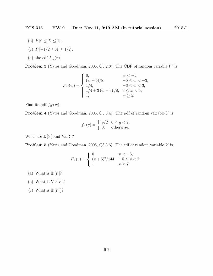
Problem 3 (Yates and Goodman, 2005, Q3.2.3). The CDF of random variable W is

FW (w) =

0, w < −5,(w + 5)/8, −5 ≤ w < −3,1/4, −3 ≤ w < 3,1/4 + 3 (w − 3) /8, 3 ≤ w < 5,1, w ≥ 5.

Find its pdf fW (w).

Problem 4 (Yates and Goodman, 2005, Q3.3.4). The pdf of random variable Y is

fY (y) =

{y/2 0 ≤ y < 2,0, otherwise.

What are E [Y ] and VarY ?

Problem 5 (Yates and Goodman, 2005, Q3.3.6). The cdf of random variable V is

FV (v) =

0 v < −5,(v + 5)2/144, −5 ≤ v < 7,1 v ≥ 7.

(a) What is E [V ]?

(b) What is Var[V ]?

(c) What is E [V 3]?

9-2

Y&G Q3.1.3Wednesday, October 03, 20123:14 PM

ECS315 2015 HW9 Page 1

Y&G Q3.3.4 Tuesday, September 07, 20102:08 PM



HW Solution 10 — Due: Nov 18, 8:59 AM

Lecturer: Prapun Suksompong, Ph.D.

Problem 1 (Randomly Phased Sinusoid). Suppose Θ is a uniform random variable on theinterval (0, 2π).

(a) Consider another random variable X defined by

X = 5 cos(7t+ Θ)

where t is some constant. Find E [X].

(b) Consider another random variable Y defined by

Y = 5 cos(7t1 + Θ)× 5 cos(7t2 + Θ)

where t1 and t2 are some constants. Find E [Y ].

Solution : First, because Θ is a uniform random variable on the interval (0, 2π), weknow that fΘ(θ) = 1

2π1(0,2π)(t). Therefore, for “any” function g, we have

E [g(Θ)] =

∫ ∞−∞

g(θ)fΘ(θ)dθ.

(a) X is a function of Θ. E [X] = 5E [cos(7t+ Θ)] = 5∫ 2π

01

2πcos(7t+ θ)dθ. Now, we know

that integration over a cycle of a sinusoid gives 0. So, E [X] = 0 .

(b) Y is another function of Θ.

E [Y ] = E [5 cos(7t1 + Θ)× 5 cos(7t2 + Θ)] = ∫ 2π0

1

2π5 cos(7t1 + θ)× 5 cos(7t2 + θ)dθ

=25

2π∫ 2π

0 cos(7t1 + θ)× cos(7t2 + θ)dθ.

10-1

ECS 315 HW Solution 10 — Due: Nov 18, 8:59 AM 2015/1

Recall1 the cosine identity

cos(a)× cos(b) =1

2(cos (a+ b) + cos (a− b)) .

Therefore,

EY =25

4π∫ 2π

0 cos (14t+ 2θ) + cos (7 (t1 − t2)) dθ

=25

4π

(∫ 2π

0 cos (14t+ 2θ) dθ + ∫ 2π0 cos (7 (t1 − t2)) dθ

).

The first integral gives 0 because it is an integration over two period of a sinusoid. Theintegrand in the second integral is a constant. So,

EY =25

4πcos (7 (t1 − t2)) ∫ 2π

0 dθ =25

4πcos (7 (t1 − t2)) 2π =

25

2cos (7 (t1 − t2)) .

Problem 2 (Yates and Goodman, 2005, Q3.4.5). X is a continuous uniform RV on theinterval (−5, 5).

(a) What is its pdf fX(x)?

(b) What is its cdf FX(x)?

(c) What is E [X]?

(d) What is E [X5]?

(e) What is E[eX]?

Solution : For a uniform random variable X on the interval (a, b), we know that

fX (x) =

{0, x < a or x > b,

1b−a , a ≤ x ≤ b

1This identity could be derived easily via the Euler’s identity:

cos(a)× cos(b) =eja + e−ja

2× ejb + e−jb

2=

1

4

(ejaejb + e−jaejb + ejae−jb + e−jae−jb

)=

1

2

(ejaejb + e−jae−jb

2+

e−jaejb + ejae−jb

2

)=

1

2(cos (a+ b) + cos (a− b)) .

10-2


and

FX (x) =

{0, x < a or x > b,x−ab−a , a ≤ x ≤ b.

In this problem, we have a = −5 and b = 5.

(a) fX (x) =

{0, x < −5 or x > 5,110, −5 ≤ x ≤ 5

(b) FX (x) =

{0, x < a or x > b,x+510, a ≤ x ≤ b.

(c) EX =∞∫−∞

xfX (x) dx =5∫−5

x× 110dx = 1

10x2

2

∣∣∣5−5

= 120

(52 − (−5)2) = 0 .

In general,

EX =

b∫a

x1

b− adx =

1

b− a

b∫a

xdx =1

b− ax2

2

∣∣∣∣ba

=1

b− ab2 − a2

2=a+ b

2.

With a = −5 and b = 5, we have EX = 0 .

(d) E [X5] =∞∫−∞

x5fX (x) dx =5∫−5

x5 × 110dx = 1

10x6

6

∣∣∣5−5

= 160

(56 − (−5)6) = 0 .

In general,

E[X5]

=

b∫a

x5 1

b− adx =

1

b− a

b∫a

x5dx =1

b− ax6

6

∣∣∣∣ba

=1

b− ab6 − a6

2.

With a = −5 and b = 5, we have E [X5] = 0 .

(e) In general,

E[eX]

=

b∫a

ex1

b− adx =

1

b− a

b∫a

exdx =1

b− aex|ba =

eb − ea

b− a.

With a = −5 and b = 5, we have E[eX]

=e5 − e−5

10≈ 14.84.

10-3


Problem 3. A random variable X is a Gaussian random variable if its pdf is given by

fX(x) =1√2πσ

e−12(x−mσ )

2

,

for some constant m and positive number σ. Furthermore, when a Gaussian random variablehas m = 0 and σ = 1, we say that it is a standard Gaussian random variable. There is noclosed-form expression for the cdf of the standard Gaussian random variable. The cdf itselfis denoted by Φ and its values (or its complementary values Q(·) = 1−Φ(·)) are traditionallyprovided by a table.

Suppose Z is a standard Gaussian random variable.

(a) Use the Φ table to find the following probabilities:

(i) P [Z < 1.52]

(ii) P [Z < −1.52]

(iii) P [Z > 1.52]

(iv) P [Z > −1.52]

(v) P [−1.36 < Z < 1.52]

(b) Use the Φ table to find the value of c that satisfies each of the following relation.

(i) P [Z > c] = 0.14

(ii) P [−c < Z < c] = 0.95

Solution :

(a)

(i) P [Z < 1.52] = Φ(1.52) = 0.9357.

(ii) P [Z < −1.52] = Φ(−1.52) = 1− Φ(1.52) = 1− 0.9357 = 0.0643.

(iii) P [Z > 1.52] = 1− P [Z < 1.52] = 1− Φ(1.52) = 1− 0.9357 = 0.0643.

(iv) It is straightforward to see that the area of P [Z > −1.52] is the same as P [Z < 1.52] =Φ(1.52). So, P [Z > −1.52] = 0.9357.

Alternatively, P [Z > −1.52] = 1 − P [Z ≤ −1.52] = 1 − Φ(−1.52) = 1 − (1 −Φ(1.52)) = Φ(1.52).

(v) P [−1.36 < Z < 1.52] = Φ(1.52)−Φ(−1.36) = Φ(1.52)−(1−Φ(1.36)) = Φ(1.52)+Φ(1.36)− 1 = 0.9357 + 0.9131− 1 = 0.8488.

10-4


(b)

(i) P [Z > c] = 1 − P [Z ≤ c] = 1 − Φ(c). So, we need 1 − Φ(c) = 0.14 or Φ(c) =1− 0.14 = 0.86. In the Φ table, we do not have exactly 0.86, but we have 0.8599and 0.8621. Because 0.86 is closer to 0.8599, we answer the value of c whoseφ(c) = 0.8599. Therefore, c ≈ 1.08.

(ii) P [−c < Z < c] = Φ(c) − Φ(−c) = Φ(c) − (1 − Φ(c)) = 2Φ(c) − 1. So, we need2Φ(c)− 1 = 0.95 or Φ(c) = 0.975. From the Φ table, we have c ≈ 1.96.

Problem 4. The peak temperature T , as measured in degrees Fahrenheit, on a July day inNew Jersey is a N (85, 100) random variable.

Remark: Do not forget that, for our class, the second parameter in N (·, ·) is the variance(not the standard deviation).

(a) Express the cdf of T in terms of the Φ function.

(b) Express each of the following probabilities in terms of the Φ function(s). Make surethat the arguments of the Φ functions are positive. (Positivity is required so that wecan directly use the Φ/Q tables to evaluate the probabilities.)

(i) P [T > 100]

(ii) P [T < 60]

(iii) P [70 ≤ T ≤ 100]

(c) Express each of the probabilities in part (b) in terms of the Q function(s). Again, makesure that the arguments of the Q functions are positive.

(d) Evaluate each of the probabilities in part (b) using the Φ/Q tables.

(e) Observe that the Φ table (“Table 4” from the lecture) stops at z = 2.99 and the Qtable (“Table 5” from the lecture) starts at z = 3.00. Why is it better to give a tablefor Q(z) instead of Φ(z) when z is large?

Solution :

(a) Recall that when X ∼ N (m,σ2), FX(x) = Φ(x−mσ

). Here, T ∼ N (85, 102). Therefore,

FT (t) = Φ

(t− 85

10

).

10-5


(b)

(i) P [T > 100] = 1− P [T ≤ 100] = 1− FT (100) = 1− Φ(

100−8510

)= 1− Φ(1.5)

(ii) P [T < 60] = P [T ≤ 60] because T is a continuous random variable and henceP [T = 60] = 0. Now, P [T ≤ 60] = FT (60) = Φ

(60−85

10

)= Φ (−2.5) =

1− Φ (2.5) . Note that, for the last equality, we use the fact that Φ(−z) =

1− Φ(z).

(iii)

P [70 ≤ T ≤ 100] = FT (100)− FT (70) = Φ

(100− 85

10

)− Φ

(70− 85

10

)= Φ (1.5)− Φ (−1.5) = Φ (1.5)− (1− Φ (1.5)) = 2Φ (1.5)− 1.

(c) In this question, we use the fact that Q(x) = 1− Φ(x).

(i) 1− Φ(1.5) = Q(1.5).

(ii) 1− Φ (2.5) = Q(2.5).

(iii) 2Φ (1.5)− 1 = 2(1−Q(1.5))− 1 = 2− 2Q(1.5)− 1 = 1− 2Q(1.5).

(d)

(i) 1− Φ(1.5) = 1− 0.9332 = 0.0668.

(ii) 1− Φ (2.5) = 1− 0.99379 = 0.0062.

(iii) 2Φ (1.5)− 1 = 2 (0.9332)− 1 = 0.8664.

(e) When z is large, Φ(z) will start with 0.999... The first few significant digits will all bethe same and hence not quite useful to be there.

Extra Questions


Problem 5. Let X be a uniform random variable on the interval [0, 1]. Set

A =

[0,

1

2

), B =

[0,

1

4

)∪[

1

2,3

4

), and C =

[0,

1

8

)∪[

1

4,3

8

)∪[

1

2,5

8

)∪[

3

4,7

8

).

Are the events [X ∈ A], [X ∈ B], and [X ∈ C] independent?

10-6


Solution : Note that

P [X ∈ A] =

12∫

0

dx =1

2,

P [X ∈ B] =

14∫

0

dx+

34∫

12

dx =1

2, and

P [X ∈ C] =

18∫

0

dx+

38∫

14

dx+

58∫

12

dx+

78∫

34

dx =1

2.

Now, for pairs of events, we have

P ([X ∈ A] ∩ [X ∈ B]) =

14∫

0

dx =1

4= P [X ∈ A]× P [X ∈ B] , (10.1)

P ([X ∈ A] ∩ [X ∈ C]) =

18∫

0

dx+

38∫

14

dx =1

4= P [X ∈ A]× P [X ∈ C] , and (10.2)

P ([X ∈ B] ∩ [X ∈ C]) =

18∫

0

dx+

58∫

12

dx =1

4= P [X ∈ B]× P [X ∈ C] . (10.3)

Finally,

P ([X ∈ A] ∩ [X ∈ B] ∩ [X ∈ C]) =

18∫

0

dx =1

8= P [X ∈ A]P [X ∈ B]P [X ∈ C] . (10.4)

From (10.1), (10.2), (10.3) and (10.4), we can conclude that the events [X ∈ A], [X ∈ B],

and [X ∈ C] are independent .

Problem 6 (Q3.5.6). Solve this question using the Φ/Q table.A professor pays 25 cents for each blackboard error made in lecture to the student who

points out the error. In a career of n years filled with blackboard errors, the total amountin dollars paid can be approximated by a Gaussian random variable Yn with expected value40n and variance 100n.

10-7


(a) What is the probability that Y20 exceeds 1000?

(b) How many years n must the professor teach in order that P [Yn > 1000] > 0.99?

Solution : We are given2 that Yn ∼ N (40n, 100n). Recall that when X ∼ N (m,σ2),

FX(x) = Φ

(x−mσ

). (10.5)

(a) Here n = 20. So, we have Yn ∼ N (40× 20, 100× 20) = N (800, 2000). For this randomvariable m = 800 and σ =

√2000.

We want to find P [Y20 > 1000] which is the same as 1 − P [Y20 ≤ 1000]. Expressingthis quantity using cdf, we have

P [Y20 > 1000] = 1− FY20(1000).

Apply (10.5) to get

P [Y20 > 1000] = 1− Φ

(1000− 800√

2000

)= 1− Φ(4.472) ≈ Q(4.47) ≈ 3.91× 10−6 .

(b) Here, the value of n is what we want. So, we will need to keep the formula in thegeneral form. Again, from (10.5), for Yn ∼ N (40n, 100n), we have

P [Yn > 1000] = 1− FYn(1000) = 1− Φ

(1000− 40n

10√n

)= 1− Φ

(100− 4n√

n

).

To find the value of n such that P [Yn > 1000] > 0.99, we will first find the value of zwhich make

1− Φ (z) > 0.99. (10.6)

At this point, we may try to solve for the value of Z by noting that (10.6) is the sameas

Φ (z) < 0.01. (10.7)

Unfortunately, the tables that we have start with Φ(0) = 0.5 and increase to somethingclose to 1 when the argument of the Φ function is large. This means we can’t directlyfind 0.01 in the table. Of course, 0.99 is in there and therefore we will need to solve(10.6) via another approach.

2Note that the expected value and the variance in this question are proportional to n. This naturallyoccurs when we consider the sum of i.i.d. random variables. The approximation by Gaussian random variableis a result of the central limit theorem (CLT).

10-8


To do this, we use another property of the Φ function. Recall that 1−Φ(z) = Φ(−z).Therefore, (10.6) is the same as

Φ (−z) > 0.99. (10.8)

From our table, we can then conclude that (10.7) (which is the same as (10.8)) willhappen when −z > 2.33. (If you have MATLAB, then you can get a more accurateanswer of 2.3263.)

Now, plugging in z = 100−4n√n

, we have 4n−100√n

> 2.33. To solve for n, we first let x =√n.

In which case, we have 4x2−100x

> 2.33 or, equivalently, 4x2− 2.33x− 100 > 0. The tworoots are x = −4.717 and x > 5.3. So, We need x < −4.717 or x > 5.3. Note thatx =√n and therefore can not be negative. So, we only have one case; that is, we need

x > 5.3. Because n = x2, we then conclude that we need n > 28.1 years .

10-9


HW Solution 11 — Due: Nov 25, 9:19 AM


Problem 1. Suppose that the time to failure (in hours) of fans in a personal computer canbe modeled by an exponential distribution with λ = 0.0003.

(a) What proportion of the fans will last at least 10,000 hours?

(b) What proportion of the fans will last at most 7000 hours?

[Montgomery and Runger, 2010, Q4-97]

Solution : See handwritten solution

Problem 2. Consider each random variable X defined below. Let Y = 1 + 2X. (i) Findand sketch the pdf of Y and (ii) Does Y belong to any of the (popular) families discussed inclass? If so, state the name of the family and find the corresponding parameters.

(a) X ∼ U(0, 1)

(b) X ∼ E(1)

(c) X ∼ N (0, 1)


Problem 3. Consider each random variable X defined below. Let Y = 1 − 2X. (i) Findand sketch the pdf of Y and (ii) Does Y belong to any of the (popular) families discussed inclass? If so, state the name of the family and find the corresponding parameters.

(a) X ∼ U(0, 1)

(b) X ∼ E(1)

(c) X ∼ N (0, 1)


11-1

HW11 Q1: Exponential RVFriday, November 21, 2014 9:02 AM

ECS315 2015 HW11 Page 1

HW11 Q2 Affine TransformationTuesday, November 11, 2014 4:15 PM

ECS315 2015 HW11 Page 2

ECS315 2015 HW11 Page 3

HW11 Q3 Affine TransformationTuesday, November 11, 2014 4:15 PM

ECS315 2015 HW11 Page 4

ECS315 2015 HW11 Page 5


Problem 4. Let X ∼ E(5) and Y = 2/X.

(a) Check that Y is still a continuous random variable.

(b) Find FY (y).

(c) Find fY (y).

(d) (optional) Find EY .

Hint: Because ddye−

10y = 10

y2e−

10y > 0 for y 6= 0. We know that e−

10y is an increasing

function on our range of integration. In particular, consider y > 10/ ln(2). Then,

e−10y > 1

2. Hence,

∞∫0

10

ye−

10y dy >

∞∫10/ ln 2

10

ye−

10y dy >

∞∫10/ ln 2

10

y

1

2dy =

∞∫10/ ln 2

5

ydy.

Remark: To be technically correct, we should be a little more careful when writingY = 2

Xbecause it is undefined when X = 0. Of course, this happens with 0 probability;

so it won’t create any serious problem. However, to avoid the problem, we may defineY by

Y =

{2/X, X 6= 0,0, X = 0.

Solution : In this question, we have Y = g(X) where the function g is defined byg(x) = 2

x.

(a) First, we evaluate P [Y = y] = P [g(X) = y].

• For each value of y 6= 0, there is only one x value that satisfies y = g(x). (Thatx value is x = 2

y.)

• When y = 0, there is no x value that satisfies y = g(x).

In both cases, for each value of y, the number of solutions for y = g(x) is countable.Therefore, we can write

P [Y = y] =∑

x:g(x)=y

P [X = x] .

Here, X ∼ E(5). Therefore, X is a continuous random variable and P [X = x] = 0 forany x. Hence,

P [Y = y] =∑

x:g(x)=y

0 = 0.

Because P [Y = y] = 0 for all y, we conclude that Y is a continuous random variable.

11-2


(b) We consider two cases: “y ≤ 0” and “y > 0”.

(i) Because X > 0, we know that Y = 2X

must be > 0 and hence, FY (y) = 0 fory ≤ 0. Note that Y can not be = 0. We need X = ∞ or −∞ to make Y = 0.However, ±∞ are not real numbers therefore they are not possible X values.

(ii) For y > 0,

FY (y) = P [Y ≤ y] = P

[2

X≤ y

]= P

[X ≥ 2

y

].

Note that, for the last equality, we can freely move X and y without worry-ing about “flipping the inequality” or “division by zero” because both X and yconsidered here are strictly positive. Now, for X ∼ E(λ) and x > 0, we have

P [X ≥ x] =

∞∫x

λe−λtdt = −e−λt∣∣∞x

= e−λx

Therefore,

FY (y) = e−5(2y ) = e

−10y .

Combining the two cases above we have

FY (y) =

{e−

10y , y > 0

0, y ≤ 0

(c) Because we have already derived the cdf in the previous part, we can find the pdf viathe cdf by fY (y) = d

dyFY (y). This gives fY at all points except at y = 0 which we will

set fY to be 0 there. (This arbitrary assignment works for continuous RV. This is whywe need to check first that the random variable is actually continuous.) Hence,

fY (y) =

{10y2e−

10y , y > 0

0, y ≤ 0.

(d) We can find EY from fY (y) found in the previous part or we can even use fX(x)

Method 1:

EY =

∫ ∞−∞

yfY (y) =

∞∫0

y10

y2e−

10y dy =

∞∫0

10

ye−

10y dy

11-3


From the hint, we have

EY >

∞∫10/ ln 2

10

ye−

10y dy >

∞∫10/ ln 2

10

y

1

2dy =

∞∫10/ ln 2

5

ydy

= 5 ln y|∞10/ ln 2 =∞.

Therefore, EY = ∞ .

Method 2:

EY = E[

1

X

]=

∞∫−∞

1

xfX (x) dx =

∞∫0

1

xλe−λxdx >

1∫0

1

xλe−λxdx

>

1∫0

1

xλe−λdx = λe−λ

1∫0

1

xdx = λe−λ lnx|10 =∞,

where the second inequality above comes from the fact that for x ∈ (0, 1), e−λx > e−λ.

Problem 5. In wireless communications systems, fading is sometimes modeled by lognor-mal random variables. We say that a positive random variable Y is lognormal if lnY is anormal random variable (say, with expected value m and variance σ2).

(a) Check that Y is still a continuous random variable.

(b) Find the pdf of Y .

Hint: First, recall that the ln is the natural log function (log base e). Let X = lnY .Then, because Y is lognormal, we know that X ∼ N (m,σ2). Next, write Y as a function ofX.

Solution :Because X = ln(Y ), we have Y = eX . So, here, we consider Y = g(X) where the function

g is defined by g(x) = ex.

(a) First, we evaluate P [Y = y] = P [g(X) = y]. Note that for each value of y, there isonly one x value that satisfies y = g(x). (That x value is x = ln(y).) So, the numberof solutions for y = g(x) is countable. Therefore, we can write

P [Y = y] =∑

x:g(x)=y

P [X = x] .

11-4


Here, X ∼ N (m,σ2). Therefore, X is a continuous random variable and P [X = x] = 0for any x. Hence,

P [Y = y] =∑

x:g(x)=y

0 = 0.

Because P [Y = y] = 0 for all y, we conclude that Y is a continuous random variable.

(b) Start with Y = eX . We know that exponential function gives strictly positive number.So, Y is always strictly positive. In particular, FY (y) = 0 for y ≤ 0.

Next, for y > 0, by definition, FY (y) = P [Y ≤ y]. Plugging in Y = eX , we have

FY (y) = P[eX ≤ y

].

Because the exponential function is strictly increasing, the event [eX ≤ y] is the sameas the event [X ≤ ln y]. Therefore,

FY (y) = P [X ≤ ln y] = FX (ln y) .

Combining the two cases above, we have

FY (y) =

{FX (ln y) , y > 0,0, y ≤ 0.

Finally, we apply

fY (y) =d

dyFY (y).

For y < 0, we have fY (y) = ddy

0 = 0. For y > 0,

fY (y) =d

dyFY (y) =

d

dyFX (ln y) = fX (ln y)× d

dyln y =

1

yfX (ln y) . (11.1)

Therefore,

fY (y) =

{1yfX (ln y) , y > 0,

0, y < 0.

At y = 0, because Y is a continuous random variable, we can assign any value, e.g. 0,to fY (0). Then

fY (y) =

{1yfX (ln y) , y > 0,

0, otherwise.

Here, X ∼ N (m,σ2). Therefore,

fX (x) =1√2πσ

e−12(x−mσ )

2

11-5


and

fY (y) =

{1√2πσy

e−12( ln(y)−m

σ )2

, y > 0,

0, otherwise.

Extra Questions

Problem 6. Cholesterol is a fatty substance that is an important part of the outer lining(membrane) of cells in the body of animals. Its normal range for an adult is 120–240 mg/dl.The Food and Nutrition Institute of the Philippines found that the total cholesterol level forFilipino adults has a mean of 159.2 mg/dl and 84.1% of adults have a cholesterol level below200 mg/dl. Suppose that the cholesterol level in the population is normally distributed.

(a) Determine the standard deviation of this distribution.

(b) What is the value of the cholesterol level that exceeds 90% of the population?

(c) An adult is at moderate risk if cholesterol level is more than one but less than twostandard deviations above the mean. What percentage of the population is at moderaterisk according to this criterion?

(d) An adult is thought to be at high risk if his cholesterol level is more than two standarddeviations above the mean. What percentage of the population is at high risk?


Problem 7. Consider a random variable X whose pdf is given by

fX(x) =

{cx2, x ∈ (1, 2) ,0, otherwise.

Let Y = 4 |X − 1.5|.

(a) Find EY .

(b) Find fY (y).


11-6

HW11 Q6: Gaussian RV - CholesterolThursday, November 13, 2014 3:49 PM

ECS315 2015 HW11 Page 6

HW11 Q7: SISOSaturday, November 22, 2014 11:54 PM

ECS315 2015 HW11 Page 7

ECS315 2015 HW11 Page 8

ECS315 2015 HW11 Page 9


HW Solution 12 — Due: Dec 2, 9:19 AM


Problem 1. Let X ∼ E(3).

(a) For each of the following function g(x). Indicate whether the random variable Y =g(X) is a continuous random variable.

(i) g(x) = x2.

(ii) g(x) =

{1, x ≥ 0,0, x < 0.

.

(iii) g(x) =

{4e−4x, x ≥ 0,0, x < 0.

(iv) g(x) =

{x, x ≤ 5,5, x > 5.

(b) Repeat part (a), but now check whether the random variable Y = g(X) is a discreterandom variable.

Hint: As shown in class, to check whether Y is a continuous random variable, we maycheck whether P [Y = y] = 0 for any real number y. Because Y = g(X), the probabilityunder consideration is

P [Y = y] = P [g (X) = y] = P [X ∈ {x : g (x) = y}] .

• At a particular y value, if there are at most countably many x values that satisfyg(X) = y, then

P [Y = y] =∑

x:g(x)=y

P [X = x].

When X is a continuous random variable, P [X = x] = 0 for any x. Therefore,P [Y = y] = 0.

Conclusion: Suppose X is a continuous random variable and there are at most count-ably many x values that satisfy g(X) = y for any y. Then, Y is a continuous randomvariable.

12-1

ECS 315 HW Solution 12 — Due: Dec 2, 9:19 AM 2015/1

• Suppose at a particular y value, we have uncountably many x values that satisfyg(X) = y. Then, we can’t rewrite P [X ∈ {x : g (x) = y}] as

∑x:g(x)=y

P [X = x] because

axiom P3 of probability is only applicable to countably many disjoint sets (cases).

When X is a continuous random variable, we can find probability by integrating itspdf:

P [Y = y] = P [X ∈ {x : g (x) = y}] =

∫{x:g(x)=y}

fX (x)dx.

If we can find a y value whose integration above is > 0 , we can conclude right awaythat Y is not a continuous random variable.

Solution :

(a)

(i) YES .

When y < 0, there is no x that satisfies g(x) = y. When y = 0, there is exactly onex (x = 0) that satisfies g(x) = y. When y > 0, there is exactly two x (x = ±√y)that satisfies g(x) = y.

Therefore, for any y, there are at most countably many x values that satisfyg(X) = y. Because X is a continuous random variable, we conclude that Y isalso a continuous random variable.

(ii) NO . An easy way to see this is that there can be only two values out of thefunction g(·): 0 or 1. So, Y = g(X) is a discrete random variable.

Alternatively, consider y = 1. We see that any x ≥ 0, can make g(x) = 1.Therefore,

P [Y = 1] = P [X ≥ 0] .

For X ∼ E(3), P [X ≥ 0] = 1 > 0.

Because we found a y with P [Y = y] > 0. Y can not be a continuous randomvariable.

(iii) YES .

The plot of the function g(x) may help you see the following facts: When y > 4or y < 0, there is no x that gives y = g(x). When 0 < y < 4, there is exactlyone x that satisfies y = g(x). Because X is a continuous random variable, we canconclude that P [Y = y] is 0 for y 6= 0.

When y = 0, any x < 0 would satisfy g(x) = y. So, P [Y = 0] = P [X < 0].However, because X ∼ E(3) is always positive. P [X < 0] = 0.

12-2


(iv) NO . Consider y = 5. We see that any x ≥ 5, can make g(x) = 5. Therefore,

P [Y = 5] = P [X ≥ 5] .

For X ∼ E(3),

P [X ≥ 5] =

∞∫5

3e−3xdx = e−15 > 0.

Because P [Y = 5] > 0, we conclude that Y can’t be a continuous random variable.

(b) To check whether a random variable is discrete, we simply check whether it has a count-able support. Also, if we have already checked that a random variable is continuous,then it can’t also be discrete.

(i) NO . We checked before that it is a continuous random variable.

(ii) YES as discussed in part (a).

(iii) NO . We checked before that it is a continuous random variable.

(iv) NO . Because X is positive, Y = g(X) can be any positive number in the interval(0, 5]. The interval is uncountable. Therefore, Y is not discrete.

We have shown previously that Y is not a continuous random variable. Here.knowing that it is not discrete means that it is of the last type: mixed randomvariable.

Problem 2. The input X and output Y of a system subject to random perturbations aredescribed probabilistically by the following joint pmf matrix:

0.02 0.10 0.08

0.08 0.32 0.40

y 2 4 5 x 1 3

Evaluate the following quantities:

(a) The marginal pmf pX(x)

(b) The marginal pmf pY (y)

(c) EX

12-3


(d) VarX

(e) EY

(f) VarY

(g) P [XY < 6]

(h) P [X = Y ]

Solution : The MATLAB codes are provided in the file P XY marginal.m.

(a) The marginal pmf pX(x) is founded by the sums along the rows of the pmf matrix:

pX (x) =

0.2, x = 10.8, x = 30, otherwise.

(b) The marginal pmf pY (y) is founded by the sums along the columns of the pmf matrix:

pY (y) =

0.1, y = 20.42, y = 40.48, y = 50, otherwise.

(c) EX =∑x

xpX (x) = 1× 0.2 + 3× 0.8 = 0.2 + 2.4 = 2.6 .

(d) E [X2] =∑x

x2pX (x) = 12 × 0.2 + 32 × 0.8 = 0.2 + 7.2 = 7.4. So, VarX = E [X2] −

(EX)2 = 7.4− (2.6)2 = 7.4− 6.76 = 0.64 .

(e) EY =∑y

ypY (y) = 2× 0.1 + 4× 0.42 + 5× 0.48 = 0.2 + 1.68 + 2.4 = 4.28 .

(f) E [Y 2] =∑y

y2pY (y) = 22 × 0.1 + 42 × 0.42 + 52 × 0.48 = 19.12. So, VarY = E [Y 2]−

(EY )2 = 19.12− 4.282 = 0.8016 .

(g) Among the 6 possible pairs of (x, y) shown in the joint pmf matrix, only the pairs(1, 2), (1, 4), (1, 5) satisfy xy < 6. Therefore, [XY < 6] = [X = 1] which impliesP [XY < 6] = P [X = 1] = 0.2 .

(h) Among the 6 possible pairs of (x, y) shown in the joint pmf matrix, there is no pairwhich has x = y. Therefore, P [X = Y ] = 0 .

12-4


Problem 3. The time until a chemical reaction is complete (in milliseconds) is approximatedby the cumulative distribution function

FX (x) =

{1− e−0.01x, x ≥ 0,0, otherwise.

(a) Determine the probability density function of X.

(b) What proportion of reactions is complete within 200 milliseconds?


Problem 4. Let a continuous random variable X denote the current measured in a thincopper wire in milliamperes. Assume that the probability density function of X is

fX (x) =

{5, 4.9 ≤ x ≤ 5.1,0, otherwise.

(a) Find the probability that a current measurement is less than 5 milliamperes.

(b) Find and plot the cumulative distribution function of the random variable X.

(c) Find the expected value of X.

(d) Find the variance and the standard deviation of X.

(e) Find the expected value of power when the resistance is 100 ohms?


12-5

Q3: pdf and cdf - chemical reactionThursday, November 13, 2014 11:07 AM

ECS315 2015 HW12 Page 1

Q4: pdf, cdf, expected value, variance - current and powerThursday, November 13, 2014 11:01 AM

ECS315 2015 HW12 Page 2

ECS315 2015 HW12 Page 3


Extra Question

Problem 5. The input X and output Y of a system subject to random perturbations aredescribed probabilistically by the joint pmf pX,Y (x, y), where x = 1, 2, 3 and y = 1, 2, 3, 4, 5.Let P denote the joint pmf matrix whose i,j entry is pX,Y (i, j), and suppose that

P =1

71

7 2 8 5 44 2 5 5 92 4 8 5 1

(a) Find the marginal pmfs pX(x) and pY (y).

(b) Find EX

(c) Find EY

(d) Find VarX

(e) Find VarY

Solution : All of the calculations in this question are simply plugging numbers intoappropriate formula. The MATLAB codes are provided in the file P XY marginal 2.m.


pX (x) =

26/71, x = 125/71, x = 220/71, x = 30, otherwise

≈

0.3662, x = 10.3521, x = 20.2817, x = 30, otherwise.

The marginal pmf pY (y) is founded by the sums along the columns of the pmf matrix:

pY (y) =

13/71, y = 18/71, y = 221/71, y = 315/71, y = 414/71, y = 50, otherwise

≈

0.1831, y = 10.1127, y = 20.2958, y = 30.2113, y = 40.1972, y = 50, otherwise.

(b) EX = 13671≈ 1.9155

(c) EY = 22271≈ 3.1268

(d) VarX = 32305041≈ 0.6407

(e) VarY = 92205041≈ 1.8290

12-6


HW Solution 13 — Due: Not Due


Problem 1. The input X and output Y of a system subject to random perturbations aredescribed probabilistically by the following joint pmf matrix:

0.02 0.10 0.08

0.08 0.32 0.40

y 2 4 5 x 1 3

(a) Evaluate the following quantities:

(i) E [XY ]

(ii) E [(X − 3)(Y − 2)]

(iii) E [X(Y 3 − 11Y 2 + 38Y )]

(iv) Cov [X, Y ]

(v) ρX,Y

Hint: Write down the formulas then use MATLAB or Excel to compute them.

(b) Find ρX,X

(c) Calculate the following quantities using the values of VarX, Cov [X, Y ], and ρX,Y thatyou got earlier.

(i) Cov [3X + 4, 6Y − 7]

(ii) ρ3X+4,6Y−7

(iii) Cov [X, 6X − 7]

(iv) ρX,6X−7

Solution : The MATLAB codes are provided in the file P XY EVarCov.m.

13-1

ECS 315 HW Solution 13 — Due: Not Due 2015/1

(a)

(i) From MATLAB, E [XY ] = 11.16 .

(ii) From MATLAB, E [(X − 3)(Y − 2)] = −0.88 .

(iii) From MATLAB, E [X(Y 3 − 11Y 2 + 38Y )] = 104 .

(iv) From MATLAB, Cov [X, Y ] = 0.032 .

(v) From MATLAB, ρX,Y = 0.044677 .

(b) ρX,X = Cov[X,X]σXσX

= Var[X]

σ2X

= 1 .

(c)

(i) Cov [3X + 4, 6Y − 7] = 3× 6× Cov [X, Y ] ≈ 3× 6× 0.032 ≈ 0.576 .

(ii) Note that

ρaX+b,cY+d =Cov [aX + b, cY + d]

σaX+bσcY+d

=acCov [X, Y ]

|a|σX |c|σY=

ac

|ac|ρX,Y = sign(ac)× ρX,Y .

Hence, ρ3X+4,6Y−7 = sign(3× 4)ρX,Y = ρX,Y = 0.0447 .

(iii) Cov [X, 6X − 7] = 1× 6× Cov [X,X] = 6× Var[X] ≈ 3.84 .

(iv) ρX,6X−7 = sign(1× 6)× ρX,X = 1 .

Problem 2. Suppose X ∼ binomial(5, 1/3), Y ∼ binomial(7, 4/5), and X |= Y . Evaluatethe following quantities.

(a) E [(X − 3)(Y − 2)]

(b) Cov [X, Y ]

(c) ρX,Y

Solution :

(a) First, becauseX and Y are independent, we have E [(X − 3)(Y − 2)] = E [X − 3]E [Y − 2].Recall that E [aX + b] = aE [X]+b. Therefore, E [X − 3]E [Y − 2] = (E [X]− 3) (E [Y ]− 2)Now, for Binomial(n, p), the expected value is np. So,

(E [X]− 3) (E [Y ]− 2) =

(5× 1

3− 3

)(7× 4

5− 2

)= −4

3× 18

5= −24

5= −4.8.

13-2


(b) Cov [X, Y ] = 0 because X |= Y .

(c) ρX,Y = 0 because Cov [X, Y ] = 0

Problem 3. Suppose we know that σX =√2110

, σY = 4√6

5, ρX,Y = − 1√

126.

(a) Find Var[X + Y ].

(b) Find E [(Y − 3X + 5)2]. Assume E [Y − 3X + 5] = 1.

Solution :

(a) First, we know that VarX = σ2X = 21

100, VarY = σ2

Y = 9625

, and Cov [X, Y ] = ρX,Y ×σX × σY = − 2

25. Now,

Var [X + Y ] = E[((X + Y )− E [X + Y ])2

]= E

[((X − EX) + (Y − EY ))2

]= E

[(X − EX)2

]+ 2E [(X − EX) (Y − EY )] + E

[(Y − EY )2

]= VarX + 2Cov [X, Y ] + VarY

=389

100= 3.89.

Remark: It is useful to remember that

Var [X + Y ] = VarX + 2Cov [X, Y ] + VarY.

Note that when X and Y are uncorrelated, Var [X + Y ] = VarX+VarY . This simplerformula also holds when X and Y are independence because independence is a strongercondition.

(b) First, we write

Y − aX − b = (Y − EY )− a (X − EX)− (aEX + b− EY )︸︷︷︸c

.

Now, using the expansion

(u+ v + t)2 = u2 + v2 + t2 + 2uv + 2ut+ 2vt,

we have

(Y − aX − b)2 = (Y − EY )2 + a2(X − EX)2 + c2

− 2a (X − EX) (Y − EY )− 2c (Y − EY ) + 2a (X − EX) c.

13-3


Recall that E [X − EX] = E [Y − EY ] = 0. Therefore,

E[(Y − aX − b)2

]= VarY + a2 VarX + c2 − 2aCov [X, Y ]

Plugging back the value of c, we have

E[(Y − aX − b)2

]= VarY + a2 VarX + (E [(Y − aX − b)])2 − 2aCov [X, Y ] .

Here, a = 3 and b = −5. Plugging these values along with the given quantities intothe formula gives

E[(Y − aX − b)2

]=

721

100= 7.21.

Problem 4. The input X and output Y of a system subject to random perturbations aredescribed probabilistically by the joint pmf pX,Y (x, y), where x = 1, 2, 3 and y = 1, 2, 3, 4, 5.Let P denote the joint pmf matrix whose i,j entry is pX,Y (i, j), and suppose that

P =1

71

7 2 8 5 44 2 5 5 92 4 8 5 1

(a) Find the marginal pmfs pX(x) and pY (y).

(b) Find EX

(c) Find EY

(d) Find VarX

(e) Find VarY

Solution : All of the calculations in this question are simply plugging numbers intoappropriate formula. The MATLAB codes are provided in the file P XY marginal 2.m.


pX (x) =

26/71, x = 125/71, x = 220/71, x = 30, otherwise

≈

0.3662, x = 10.3521, x = 20.2817, x = 30, otherwise.

13-4


The marginal pmf pY (y) is founded by the sums along the columns of the pmf matrix:

pY (y) =

13/71, y = 18/71, y = 221/71, y = 315/71, y = 414/71, y = 50, otherwise

≈

0.1831, y = 10.1127, y = 20.2958, y = 30.2113, y = 40.1972, y = 50, otherwise.

(b) EX = 13671≈ 1.9155

(c) EY = 22271≈ 3.1268

(d) VarX = 32305041≈ 0.6407

(e) VarY = 92205041≈ 1.8290

Problem 5. A webpage server can handle r requests per day. Find the probability thatthe server gets more than r requests at least once in n days. Assume that the number ofrequests on day i is Xi ∼ P(α) and that X1, . . . , Xn are independent.

Solution : [Gubner, 2006, Ex 2.10]

P

[n⋃i=1

[Xi > r]

]= 1− P

[n⋂i=1

[Xi ≤ r]

]= 1−

n∏i=1

P [Xi ≤ r]

= 1−n∏i=1

(r∑

k=0

αke−α

k!

)= 1−

(r∑

k=0

αke−α

k!

)n

.

Extra Questions

Problem 6. Suppose X ∼ binomial(5, 1/3), Y ∼ binomial(7, 4/5), and X |= Y .

(a) A vector describing the pmf of X can be created by the MATLAB expression:

x = 0:5; pX = binopdf(x,5,1/3).

What is the expression that would give pY, a corresponding vector describing the pmfof Y ?

13-5


(b) Use pX and pY from part (a), how can you create the joint pmf matrix in MATLAB? Donot use “for-loop”, “while-loop”, “if statement”. Hint: Multiply them in an appropriateorientation.

(c) Use MATLAB to evaluate the following quantities. Again, do not use “for-loop”, “while-loop”, “if statement”.

(i) EX(ii) P [X = Y ]

(iii) P [XY < 6]

Solution : The MATLAB codes are provided in the file P XY jointfromMarginal indp.m.

(a) y = 0:7; pY = binopdf(y,7,4/5);

(b) P = pX.’*pY;

(c)

(i) EX = 1.667

(ii) P [X = Y ] = 0.0121

(iii) P [XY < 6] = 0.2727

Problem 7. Suppose VarX = 5. Find Cov [X,X] and ρX,X .

Solution :

(a) Cov [X,X] = E [(X − EX)(X − EX)] = E [(X − EX)2] = VarX = 5 .

(b) ρX,X = Cov[X,X]σXσX

= VarXσ2X

= VarXVarX

= 1 .

13-6

ecs 315: probability and random processes 2015/1 …...so, xis a binomial rv. problem 3. arrivals of...

Documents