1

Economy-wide Cost of Electricity Load Shedding in Nepal1,2

Govinda Timilsina, Jevgenijs Steinbuks and Prakash Sapkota3

Abstract: This study estimates the economic costs of electricity load shedding in Nepal over

the period 2008–16. We show that in the absence of load shedding, annual gross domestic

product, on average, would have been almost 7 percent higher than it was during the period of

power outages. The load shedding particularly strongly affected investment that would have been

48 percent higher with the reliable power supply. Although reliability of power supply in the

residential sector has recently improved because of better electricity load management, and an

increase in electricity production and imports, the industrial sector still faces significant load

shedding. Unless the electricity load shedding is eliminated, Nepal will continue to suffer a

heavy economic loss.

Key Words: Electric power outages, Electricity load shedding, Electricity supply, Economic

growth, Nepal

JEL: C22, C68, O53, Q43

1 The opinions expressed in this paper are of authors and should not be attributed to the World Bank Group and the

organizations they are affiliated with. 2 An earlier version of the study has been published as a World Bank Policy Research Working paper (Timilsina et

al. 2018). The working paper version considers only CGE analysis and does not consider the econometric analysis

included in this study. 3 Timilsina (gtimilsina@worldbank.org) is the corresponding author. Timilsina and Steinbuks are, respectively,

Senior Economist and Economist at the Development Research Group of the World Bank. Sapkota was a consultant

to the World Bank during this study.

2

Economy-wide Cost of Electricity Load Shedding in Nepal

1. Introduction

Nepal, a small country on the lap of the Himalayas, is one of the poorest countries in the

world in terms of infrastructure and economic development. In 2013, per capita electricity

consumption in Nepal, for example, was 427 times lower than that in Iceland, the country with

the highest per capita electricity consumption in the world; 182 times lower than that in Norway,

a country with hydropower as the primary source for electricity supply, like Nepal; 101 times

lower than that in the United States; 81 times lower than that in the Republic of Korea; 30 times

lower than that in China; and 6 times lower than that in neighboring India.4 As of January 31,

2018, Nepal has about 1,000 MW of power generation capacity for its almost 30 million

population. Of this total installed capacity, which is mostly run-of-river type, 70% is not

available during the dry season (March-April). The lack of electricity generation capacity and

further unavailability of the existing capacity due to very low river discharge in the dry season,

combined with poor electricity load management and growing demand for electric power

resulted in a huge load shedding over the decade starting in 2008. In the dry season in 2015 and

2016, the country faced up to 14 hours of load shedding in a typical day.5

More recently, starting from 2017, the situation has improved and regular electricity

supply to households in major urban areas, including the capital city, Kathmandu, has been

resumed. Several factors, including an innovative load management system adopted by the state

electricity utility - Nepal Electricity Authority, increased domestic supply due to commissioning

4 Calculated based on data from the World Bank’s online database available at http://databank.worldbank.org/data/home.aspx. 5 The Himalayan Times, January 03, 2016. https://thehimalayantimes.com/kathmandu/.

3

of a few new power plants and increased imports of electricity from India facilitated by the

completion of a 400 KV, 1,000 MW cross-border transmission line. However, many parts of the

country still face load shedding, and demand for industrial customers is still unmet. In a personal

communication, representatives from the Federation of Nepalese Chambers of Commerce and

Industry (FNCCI) of Nepal claim that the current industrial sector load alone exceeds 3,000 MW,

whereas the country has less than 1,000 MW of total installed capacity. Lack of reliable grid

electricity supply increases the production costs of larger industrial firms and adversely affects

their competitiveness, as they have to rely on more expensive diesel-based captive generation (or

self-generation) for their electricity supply (Foster and Steinbuks, 2008; Steinbuks and Foster

2010). For small and medium enterprises, lack of quality electricity supply is even greater

problem for their business, as they often financially constrained and cannot afford captive power

generation (Steinbuks, 2012). Thus, lack of adequate electricity supply capacity and load

shedding are one of the major barriers to Nepal’s economic development and its goal to alleviate

poverty.

The purpose of this study is to assess the economic costs of electricity load shedding in

Nepal, specifically accounting for:

(i) Firms’ direct costs resulting from the industrial output loss due to lost shedding.

These costs are especially large for small and medium size enterprises that cannot

afford expensive back-up systems;

(ii) Firms’ indirect costs resulting from diminished investment in the electricity-intensive

capital.

(iii) Households’ costs of purchasing imported backup technologies, such as batteries and

inverters.6

6Due to data limitations we do not explicitly account for households’ direct utility loss resulting from power outages, such as e.g., their impeded ability to access lighting, media and telecommunication services.

4

Our paper relates to several earlier studies that attempt to estimate the economic costs of

load shedding in Nepal (see e.g., Jyoti et al., 2006, and Shrestha, 2010). However, these studies

have narrow scope as they focus only on the loss of power sales from the utility. They do not

account for either direct economic costs due to the disruption of production in the manufacturing

and service sectors or for any indirect economic losses. This study aims to contribute in filling

this research gap.

Beyond the specific context of Nepal, the study is also contributes to the growing body of

literature assessing economic costs of unreliable electricity supply. Many studies have estimated

the cost of unreliable power supply in both developed and developing economies. Key studies

include Foster and Steinbuks (2009), Steinbuks and Foster (2010), Abdullah and Mariel (2010),

Braimah and Amponsah (2012), Kaseke and Hosking (2012), Steinbuks (2012), Oseni and Pollitt

(2013), Chakravorty et al., (2014), Fisher-Vanden et al., (2015), Allcott et al (2016), and Oseni

(2017). Some of these studies deal with unplanned electricity outages and use a methodology

where potential consumers are surveyed asking their willingness to pay (WTP) to have reliable

supply of electricity. For example, Abdullah and Mariel (2010) use a choice experiment method

to determine the willingness to pay for improved electricity services, surveying 200 households

in Kisumu District, Kenya. Braimah and Amponsah (2012) survey 320 micro and small

industries from three industrial clusters within the Kumasi metropolis in Ghana to explore the

relationship between frequent and unscheduled electricity outages to micro and small-scale

industries. Bose et al. (2006) use a two-stage random sampling survey of 500 manufacturing

firms and 900 farmers to assess willingness to pay for reliable supply of electricity in Karnataka

in India. Oseni (2017) uses data collected from a sample of Nigerian households, and the results

of his econometric analysis reveals that engagement in self-generation is positively correlated

5

with WTP for reliability. These studies are different from the current study in two respects. First,

they deal with unplanned electricity outages and do not necessarily deal with the planned outages

or load shedding the current study is investigating. Second, these studies estimate only direct

economic costs of not getting a reliable supply of electricity. These studies thus are not able

assess the overall economic costs of either unreliable supply or electricity supply shortages.

Other studies, such as Steinbuks and Foster (2010), Kaseke and Hosking (2012), Oseni

and Pollitt (2013), Chakravorty et al., (2014), Fisher-Vanden et al., (2015), and Allcott et al.,

(2016) assess econometrically the impacts of electricity outages or load shedding. Kaseke and

Hosking (2012) estimate the economic costs of load shedding in the mining sector in Zimbabwe.

Steinbuks and Foster (2010) and Oseni and Pollitt (2013) estimate economic costs of unreliable

power supply using cross-sectional data on electricity outages collected by the World Bank

Enterprise Survey in African countries. Chakravorty et al., (2014) estimate the returns to

household income due to improved access and reliability of electricity based on a representative

panel of more than 10,000 households in rural India. Fisher-Vanden et al., (2015) use a large

panel of 23,000 energy-intensive Chinese firms to examine how firms responded to severe power

shortages in the early 2000s. Allcott et al., (2016) analyze the impacts of weekly “power

holidays” or load shedding in the manufacturing industry in India. All these studies analyze only

partial equilibrium effects of unreliable power supply and capture only the direct costs of load

shedding. They do not include the economic costs due to interlinkages of industries and

6

economic agents.7 These indirect impacts are important because, depending upon the structure of

an economy, the size of indirect impacts could be higher than the size of direct impacts.

To assess the economic costs of load shedding in Nepal we use a computable general

equilibrium (CGE) model. This CGE model can capture both direct and indirect economy-wide

effects of load shedding’s. The load shedding either constrains supply of electricity for firms or

households, or increases costs of electricity service. This, in turn, results in reduction of

electricity use and higher costs of output of electricity-intensive industries. This further increases

the output prices of other industries that rely on domestic inputs produced by energy-intensive

industries. As a result, the overall output of the economy is curtailed and prices of most goods

and services of domestic industries do rise. Households’ utility falls both directly (from

consumption of unreliable electricity), and indirectly (as they face higher prices of other goods

and services). Also, as domestic production becomes more expensive as compared to their

international counterparts, domestic industries become less competitive and exports fall. Our

CGE model accounts for all these effects of load shedding.

To validate the results of CGE model, we also estimate vector error correction model

(VECM) of co-integrated electricity consumption and GDP variables. Using VECM estimates

we conduct impulse response analysis to evaluate GDP response to power outage shocks.

Nepal could not meet, on average, 20 percent of its total electricity demand in each year

over the period 2008-2016. Our analysis suggests that if the power supply was reliable over that

period, Nepal’s GDP would have been 7 percent higher, the total investment would have been 48 7Fisher-Vanden et al., (2015) capture some cross industry effects by finding that Chinese firms re-optimize among

inputs to production by substituting materials for energy. Their analysis, however, does not investigate any general

equilibrium effects.

7

percent higher, and the total sectoral output would have been 7.5 percent higher. Both imports

and exports would have also increased.8 We also find that relying on diesel fired back-up

systems to avoid load shedding has a relatively small effect on reducing economic costs of load

shedding in Nepal.

The rest of the paper is organized as follows. Section 2 briefly presents the CGE model

and econometric framework used for its validation, followed by a brief description of data in

Section 3. Section 4 describes the simulated load shedding scenarios. Section 5 presents and

discusses key results. Section 6 concludes and draws some policy remarks.

2. Analytical Framework

Below we describe two different methods that we use to assess the economic effects of

load shedding in Nepal. We first show the computable general equilibrium (CGE) model to

quantify economic effects of load shedding. We then present the time-series vector error

correction model (VECM) we employ to validate the predictions of the CGE model.

2.1 CGE Model

We use a single country static general equilibrium model that is calibrated based on Nepal social

accounting matrix (see section 3). This is a standard CGE model with detailed representation of

factor markets, product markets and household welfare. It follows the rich literature on single

country CGE modeling, such as Shoven and Whalley (1984, 1992), Coady and Harris (2001),

and Decaluwé et al. (2005). The structure of the model is briefly described below. The detailed

description of the model is available in Timilsina et al. (2018). 8Falling oil prices after 2014 may have lowered the costs of load shedding (both direct and indirect) for two years

out of ten years considered in the analysis. However, capturing this effect is complicated and beyond the scope of

this paper analysis.

8

Figure 1: Simplified structure of modeling production sectors

9

Sectoral production: For this analysis, we consider 15 sectors.9 The production structure of

agriculture and non-agriculture sectors is differentiated because land is the main input in the

agriculture sector, and not in the other sectors. Figure 1 illustrates the basic structure of modeling

the production sector. At the highest nesting level of the production structure, sectoral output is a

constant elasticity of substitution (CES) combination of sectoral value added and total

intermediate inputs. While a sectoral value added is CES combination of labor and capital inputs,

total intermediate input is a Leontief aggregate of individual intermediate inputs.10 The capital in

the agriculture sector is a Cobb-Douglas function combining agricultural capital and land. The

composite labor is a CES aggregate of skilled and unskilled labors in each sector. This

hierarchical nested specification allows different scale of substitution among primary factors

(Despotakis, 1980).

Foreign trade: We divide imports into competitive and non-competitive categories. We model

the competitive imports with Armington assumptions (Armington, 1969) and non-competitive

imports with the Leontief fixed coefficient technology. For a competitive or tradable good, we

derive import demand based on a CES combination of a domestically produced component and

an imported component. We use a constant elasticity of transformation (CET) function to

allocate total domestic production or domestic output of a good or service to domestic

consumption and exports. The standard small-country assumption implies that no good or service

produced in Nepal can affect the international price of that good or service. 9 The number of sectors and commodities can be changed as needed. For the sake of clarity, we further aggregated

the sectors when results are presented and discussed. For example, five agriculture (crop) sectors, and a forestry

sector are combined into single ‘agriculture and forestry’ sector. 10Leontief specification does not allow substitution between intermediate consumption in a production sector. Since

this specification does not allow structural adjustment through input substitutions, the reported impacts are likely

overestimated. More flexible forms, such as CES, resolve this issue. However, key parameters of the CES

specification, particularly the elasticity of substitution, are not available.

10

Households and government: We use Stone-Geary linear expenditure function11 to model

household consumption. We compute Hicksian equivalent variation to measure household

welfare effects of counterfactual simulation, here the “load shedding” scenario. We derive

household savings based on exogenously specified marginal propensity to consume. Government

collects taxes, makes public expenditures and saves, receives and provides transfers.

Macroeconomic closure: The model we develop for this analysis is a static model, where the

investment rate is assumed to be in its steady state. Total investment is financed through

domestic savings (household savings, government savings, firm’s savings) and foreign savings

(or borrowing from foreign countries or institutions). The supplies of primary factors (i.e., labor,

capital and land) are fixed for a given year. For labor, in fact, the working-age population for a

given year is exogenous and fixed. However, the model allows labor to move across the sectors.

The agricultural capital is mobile (can be moved from one crop to another based on their

profitability) while industrial capital is sector specific. The model closes keeping foreign saving

(current account balance) as exogenous. The exchange rate is fixed and the real exchange rate

acts as the price numeraire.

2.2 Vector Error Correction Model

To validate the results of the CGE model, we estimate a vector error correction model

(VECM), where electricity consumption and GDP are simultaneously determined. The VECM is

a framework for estimation, inference, and forecasting of difference stationary multivariate time

11 The Stone-Geary function is appropriate representation of household demand when households have a

“subsistence” level of consumption irrespective of the prices of goods for subsistence consumption and household

income. After subsistence quantities are satisfied, households choose further consumption based on standard

microeconomic assumptions. It serves as a basis for the linear expenditure system (LES) of consumer demand

(Stone, 1954; Frisch, 1954).

11

series, which has been extensively used in the energy economics literature.12 A brief formal

representation of the VECM is documented below. For advanced textbook treatment of the

VECM, please refer to Lütkepohl (2005) and Enders (2010). Before estimating the VECM we

need to establish that electricity and GDP series are difference stationary. To test for this

hypothesis we run four popular unit-root tests: (i) the Augmented Dickey-Fuller (or ADF) test

(Dickey and Fuller, 1979), (ii) the modified Dickey–Fuller (or DF-GLS) test (Elliott et al., 1996),

the Phillips and Perron (1988) test, and the KPSS test (Kwiatkowski et al., 1992). We then

estimate the VECM, whose general form representation with lag order p is given by

𝚫 𝐲𝐭 = 𝚷 𝐲𝐭!𝟏 + 𝚪𝐢𝒑!𝟏𝒊!𝟏 𝚫 𝐲𝐭!𝟏 + 𝐁𝐱𝐭 + 𝛜𝐭 (1)

where yt is the K×1 vector of endogenous variables (i.e., electricity consumption and output,

both in natural logarithms), Π, Γi and B are matrices of coefficients, xt is the M×1 vector of

exogenous variables, and 𝛜𝐭 is the K×1 vector of white noise innovations. As we are primarily

interested in the dynamics of electricity-GDP relationship, we do not include any exogenous

terms, so the third term on the right hand side of equation (1) disappears. We set the maximum

number of lagged terms, p, and equal to four, and choose the optimal number of lags based on

Schwarz/Bayesian Information Criterion (BIC). If the variables yt are difference stationary, the

matrix Π in equation (1) has rank 0 ≤ r<K, where r is the number of linearly independent

cointegrating vectors. As matrix Π has reduced rank the cointegrating vectors are not identified

without further restrictions. We apply standard normalization restrictions suggested by Johansen

(1995). After the VECM is estimated we test for cointegration via Johansen’s max-eigenvalue

statistic and trace statistic. We also evaluate the stability of the estimated VECM by testing if the

12Bruns et al. (2014), Ozturk (2010) and Payne (2010) are good surveys of this literature.

12

moduli of the remaining r eigenvalues are strictly less than unity. After all robustness checks are

performed, we calculate impulse response functions (IRFs) to measure the effects of a shock to

electricity consumption on GDP. As the simple IRFs give biased results when the shocks are

contemporaneously correlated, we follow the standard literature (see e.g., Sims, 1980) and

perform Cholesky decomposition to orthogonalize the covariance matrix of shocks.

3. Data

To calibrate the CGE model, we use the social accounting matrix (SAM) of year 2007,

which was prepared based on GTAP database. We use the 2007 SAM by design, because this is

the last year when there was no load shedding. The market for electricity services was cleared,

and all sectors and households have received the full demanded amount of electricity services.

After 2007, when load shedding started, a SAM may misrepresent electricity input because:

(i) the technical or input-output coefficient likely overestimates the marginal product of

electricity input in a sector;

(ii) a portion of the technical coefficient for electricity (i.e., ratio of output from sector to

its electricity input) may have diverted to oil if the sector used captive power running

its own diesel fired backup generators.

The SAM of any year after 2007 thus needs an adjustment if used for this type of

analysis. The SAM of 2007 serves as a benchmark for the analysis of the economic impact of

load shedding. All share parameters and other parameters are calibrated based on the 2007 SAM.

The values of the elasticity of substitution in the CES and CET nests are based on the CGE

modeling literature (see e.g., Timilsina and Shrestha, 2002; Timilsina et al. 2018).

13

The time-series data for the econometric CGE model validation comes from two sources.

The net electric power consumption (i.e., excluding transmission, distribution, and

transformation losses) series come from the IEA World Energy Statistics and Balances database

(IEA, 2017). The GDP series (in 2010 US dollars) come from the World Bank World

Development Indicators (WDI) database. Both series are available starting from 1971. We

estimate the VECM over the period 1971-2007, when the power supply was reliable.

4. Designing the Load Shedding and Back-up Supply Scenarios

We consider two scenarios. The first scenario reflects the real situation of load shedding

occurred during the 2007-2016 period. This is the main scenario as this is the focus of the

analysis. The second is a hypothetical scenario that assumes what would happen if the load

shedding were avoided through diesel-based generation back -ups operated by the utility.

Table 1 presents electricity supply and demand balance for over the 2007-2016 period,

which is the basis of the main scenario. In 2007, the electricity supply met the demand. After

2007, the electricity supply is always lower than the demand for electricity, thereby causing load

shedding. For year 2008, the electricity deficit was 9 percent of the demand. Between 2009 and

2014, the supply deficit was around 20 percent of the demand. Though for 2015 and 2016 we

could not obtain electricity requirement data and thus calculate deficit, we know that it was

higher than in previous years as the country faced most serious load shedding. We assume that,

on average, 20 percent of the annual demand for electricity was not met by the supply.

Therefore, we simulate the economic effects of a 20 percent reduction in electricity supply in

each year.

Table 1. Electricity supply and demand balance in Nepal during 2007-2016 (GWh)

14

Year NEA

Supply IPP

Supply Domestic

Supply Import Total

supply Demand Deficit %

Deficit 2007 1,761 329 2,090 962 3,052 3,000

2008 1,802 425 2,228 958 3,186 3,490 -304 -9% 2009 1,849 356 2,205 926 3,131 3,859 -728 -19% 2010 2,122 639 2,760 591 3,352 4,367 -1,015 -23% 2011 2,125 694 2,820 1,039 3,858 4,833 -975 -20% 2012 2,359 746 3,105 1,074 4,179 5,195 -1,016 -20% 2013 2,292 790 3,082 1,176 4,258 5,446 -1,188 -22% 2014 2,298 1,319 3,617 1,070 4,687 5,909 -1,222 -21% 2015 2,367 1,370 3,737 1,269 5,006 n.a. n.a. n.a. 2016 2,168 1,173 3,342 1,758 5,100 n.a. n.a. n.a.

Source: Nepal Electricity Authority (NEA). Annual Reports for the period between 2007 and 2017.

One of the limitations of shocking the load shedding under this scenario is that it does not

capture captive power generation to back up electricity supply during the load shedding. While

not all industries can afford backup power generation, large industries invest in backup power

supply. In such a case, large industries would not cut their production during the load shedding,

instead they pay a higher price for electricity supplied through the backup system. Unfortunately,

we do not have the detailed data on the captive power generation capacities and their utilization.

Moreover, households also use devices (e.g., invertors), which store electricity when electricity

supply is available and dissipate the stored electricity for certain applications (e.g., lighting, cell

phone charging) when there is load shedding. Again, we do not have detailed data on the stock

and utilization of storage devices. To fully capture the economic implications of captive power

and storage devices that could have been used to fully avoid load shedding, we design a

hypothetical ‘back-up’ scenario.

This hypothetical scenario assumes that diesel-fired generators are installed in the

electricity sub-stations to supply power when hydropower, the main source of electricity in

Nepal, is not available. In this scenario, we assume that the 20% of shortage of annual electricity

demand can be met using diesel fired back up generators. Using necessary data, such as

15

overnight construction costs (US$600/kW for diesel and US$2,200/kW for hydro), average

diesel price (US$ 0.96/liter), heat rate of diesel fired plants (10.55GJ/KWh/), capacity factors

(85% for diesel plants and 50% for hydro plants), economic lives (20 years for diesel plants and

40 years for hydro plants) and discount rate (7%), we estimate levelized costs of diesel fired

power generation (US$297/MWh), and hydro power generation (US$41/MWh). When the total

electricity mix accounts for 20% of diesel-based generation and 80% of hydro generation, the

supply costs would be 2.25 times {(0.2*299+0.8*41)/1.0* 41} higher than when the entire

electricity is supplied by hydroelectric sources. In other words, the price of electricity would

have been 2.25 times higher with the diesel back-up system to avoid the load shedding.

5. Results

This section describes the main findings of our analysis. We first show estimates of the

direct costs of load shedding, followed by the results of simulated CGE model scenarios and

their validation based on the VECM model.

5.1 Direct costs of load shedding

We assess the direct economic costs of electricity load shedding by calculating the value

of lost sales. Using the electricity deficit in a given year and the average price of electricity in

that year we calculate the monetary value of lost electricity sales due to the load shedding

(Figure 2). The white columns in Figure 2 show the value of electricity losses at current prices;

the back columns represent the value of losses in 2016 constant prices. The value of electricity

loss (in current prices) have increased every year, starting from US$ 31.8 Million in 2008 to US$

117.6 Million in 2016. The total current price value of electricity loss due to load shedding

during 2008-2016 period amounts to US$770 Million. If the loss is expressed in 2016 prices, it

amounts to US$ 833 Million.

16

Figure 2. Direct costs of electricity load shedding in Nepal (Million US$)

5.2 CGE model results

5.2.1 Scenario with no back up power generation

Figure 3 presents the effects of load shedding on key macroeconomic variables in the

scenario where the electricity shortages cannot be avoided. The results are expressed as the

average annual deviation compared to a hypothetical situation where load shedding would not

have occurred.

The results reveal that load shedding caused a reduction of 6.4% of annual GDP, on

average, during the 2008-2016 period. This means if there were no load-shedding annual GDP

would have been almost 7 percent higher, on average, as compared to what it was during the

31.1

63.6

92.0

90.7

84.4

93.2

87.5

109.

8

117.

6

38.3

83.3

106.

9

93.5

89.2

98.0

94.8

111.

7

117.

6

2008 2009 2010 2011 2012 2013 2014 2015 2016

Current price 2016 price

Total loss during the 2008-2016 in current price = US$ 770 Million Total loss during the 2008-2016 in 2016 price = US$ 833 Million

17

2008-2016 period.13 The worst impacts can be observed on the investment side. The load

shedding caused almost 33 percent loss of investment demand as compared to the baseline. In

other words, if there were no load shedding, the average annual investment would be more than

48% higher as compared to the level during 2008-2015. Due to the lower investment and

production loss caused by the load shedding, total industrial outputs decreased by almost 7%. As

production activities decrease, international trade would also decrease; due to the load shedding,

annual exports and imports were estimated to be decreased by, on average, 2.8% and 5.4%,

respectively during the 2008-2016 period.

Figure 3: Impacts on key macroeconomic variables

Annual average deviation from the CGE model baseline (%) during the 2008-2015 period

13This means the actual GDP (with load shedding) is 6.4% smaller as compared to the baseline (without load-shedding). If we consider the actual GDP, with the load shedding, as the base, the hypothetical GDP would be [{100/(100-6.4)}-1]*100 = 6.9%.

-6.4

-2.5

-32.6

-6.9-5.4

-2.8

Grossdomesticproducts

Governmentrevenue

Investmentdemand

Totalindustrialoutput Imports Exports

18

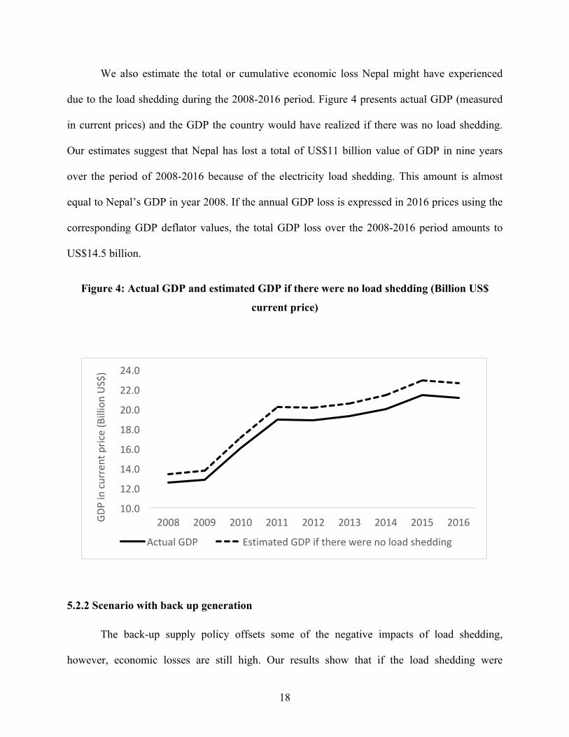
We also estimate the total or cumulative economic loss Nepal might have experienced

due to the load shedding during the 2008-2016 period. Figure 4 presents actual GDP (measured

in current prices) and the GDP the country would have realized if there was no load shedding.

Our estimates suggest that Nepal has lost a total of US$11 billion value of GDP in nine years

over the period of 2008-2016 because of the electricity load shedding. This amount is almost

equal to Nepal’s GDP in year 2008. If the annual GDP loss is expressed in 2016 prices using the

corresponding GDP deflator values, the total GDP loss over the 2008-2016 period amounts to

US$14.5 billion.

Figure 4: Actual GDP and estimated GDP if there were no load shedding (Billion US$

current price)

5.2.2 Scenario with back up generation

The back-up supply policy offsets some of the negative impacts of load shedding,

however, economic losses are still high. Our results show that if the load shedding were

10.0

12.0

14.0

16.0

18.0

20.0

22.0

24.0

2008 2009 2010 2011 2012 2013 2014 2015 2016GDPincurrentprice(BillionUS$)

ActualGDP EstimatedGDPiftherewerenoloadshedding

19

completely avoided through back-up electricity generation, the country would still suffer a 3.4

percent GDP loss. The total sectoral output decreases by 5.4 percent and total consumption of the

households by 3.8 percent. The main reason behind these economic losses is that the expensive

diesel fired back-up system increases electricity supply costs and, therefore price of electricity,

by 225 percent. This result suggests that expensive diesel-based back-up electricity supply

system to avoid load shedding can only to a limited extent mitigate economic costs of load

shedding in Nepal.

5.2 CGE Model Validation Using VECM

In this section we discuss the diagnostics and the results of the estimated VECM model to

validate the CGE model predictions. We start with the results of the four unit root tests (see

Appendix Table A.1). The ADF, DF-GLS and Phillips-Perron tests all cannot reject the null of

unit root, whereas the KPSS test rejects the null of stationary series. We can thus conclude that

both GDP and electricity consumption series are non-stationary.

We then evaluate the estimated coefficients of the VECM equations (see Appendix Table A.2).

In the GDP equation, the lagged error correction term, ECT, is negative and statistically

significant, representing the negative feedback necessary in real GDP to bring the electricity

consumption back to equilibrium. The lagged coefficients in this equation are also negative and

significantly different from zero. In the electricity consumption equation, as expected, the lagged

error correction term is positive. That is, if the electricity to GDP ratio (or electricity intensity) is

above it long-run equilibrium, either GDP must fall or electricity consumption must increase.

The short-run coefficients are not significant, with an exception of second lag of electricity

consumption, which is positive and statistically significant from zero.

20

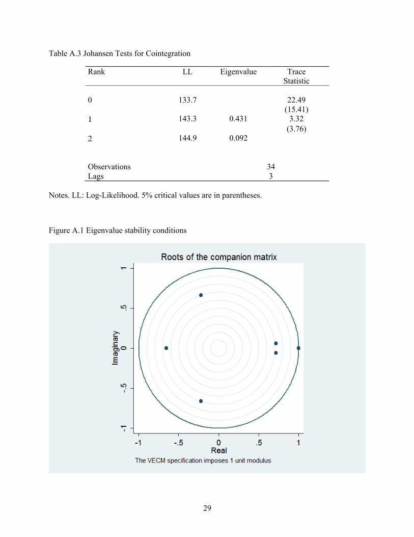
As regards the diagnostic tests, we observe the results of Johansen tests for cointegration (see

Appendix Table A.3). The trace statistic indicates that we can reject the null of 0 cointegrating

vectors, and cannot reject the null of 1 cointegrating vector. We can thus conclude that there is

one cointegrating vector. We also see that the moduli of the remaining five eigenvalues are

strictly less than unity (Appendix Figure A.1). The eigenvalues thus meet the VECM stability

condition.

Figure 5: Cumulative Orthogonalized Impulse Responses

Finally, we conduct the impulse response analysis to measure the reaction of electricity

consumption and GDP to the exogenous shock at the time of the shock and over subsequent

points in time. Figure 7 and Table A.4 show cumulative orthogonolized impulse response

21

(OIRF) functions, which plot the accumulation of the impact of the shock to electricity

consumption and GDP across time. We compute the OIRF up to 10 periods ahead. Figure 5

shows that electricity consumption is positively affected by a GDP shock both upon impact and

that as time goes on (lower left panel). GDP does not immediately respond to the electricity

consumption shock, however, it does increase as the time goes on. Table A.4 shows that over 10

periods, a 1 percent increase (decline) in electricity consumption cumulatively results in a 0.045

percent increase (decline) in GDP. Following the assumption in the CGE model that Nepal has

experienced a 20% deficit in electricity consumption over the consecutive period of nine years,

the cumulative effect of power supply deficit based on the VECM impulse response analysis

comes to about 8 percent decline in GDP. This is in line with the CGE model predictions.

6 Conclusions and Further Remarks

Over the last 10 years, electricity load shedding created severe welfare losses to

households and posed a major barrier to economic development in Nepal. The problem started in

2008 and peaked in 2016 when the country faced up to 14 hours of power cuts in the dry (winter

and spring) season. Recently, the situation has improved for residential consumers. However,

industrial consumers are still facing load shedding that causes either production cuts or increased

production costs due to adoption of expensive self-generation systems.

Our study estimates that Nepal has lost a total of US$11 billion value of GDP in nine

years over the period of 2008-2016 due to electricity load shedding. This amount is almost equal

to Nepal’s GDP in 2008. If the annual GDP loss is expressed in 2016 prices based on

corresponding GDP deflator values, the total GDP loss over the 2008-2016 period amounts to

22

US$14.5 billion. On average, the country lost more than 6% of its GDP annually during that

period. All sectors experienced cuts in their outputs, due to either lack of electricity supply

(small and medium sized industries which cannot afford back-up power) or increased electricity

costs (e.g., large industries which can afford expensive back-up generation). Load shedding has

particularly strongly affected investment. Our analysis suggests that in the absence of load

shedding, annual investment, on average, would have increased by 48 percent during the 2008-

2016 period. Lower investment and corresponding production losses caused by the load shedding

resulted in a 6.9 percent decrease in the industrial output. Nepal’s international trade has been

also affected. Over the period of 2008-2016, the load shedding caused a 2.8 percent reduction in

exports and 5.4 percent reduction in imports. Our results also suggest that the diesel-fired back-

up system to avoid load shedding could only to a small extent reduce the economic costs of load

shedding in Nepal.

As the estimated effects are based on the CGE model simulations rather than on a panel

data econometric analysis with credible identification strategy, the numbers presented in this

study should be interpreted with caution. These results are indicative also because the estimates

change, though not significantly, if some model parameters, such as the elasticity of substitution,

are altered. Also, the effects of load shedding are only relevant for the customers already

connected to the national electricity grid and does not fully include economic loss in many areas

not served by the national grid or off-grid/distributed generation systems. This study also does

not account for economic losses of not avoided greenfield investment in large-scale electricity

intensive industries, such as fertilizer factories, chemical industries. A further investigation

would be needed to assess the extent to which these potentially confounding factors are

significant.

23

All in all, while the recent reduction of load shedding in the residential sector has

certainly helped reduce the welfare losses faced by households, the economic losses would still

persist because industries are continuously facing load shedding or higher electricity expenditure

due to expensive back-up supply provisions. A complete elimination of load shedding,

particularly from the industrial sector, is crucial to avoid millions of dollars of economic loss in

years to come.

Acknowledgement

The authors would like to thank Xiaoping Wang, Sheoli Pargal, Fan Zhang, Kene Ezemenari,

Damir Cosic, Faris H. Hadad-Zervos and Mike Toman for their valuable comments and

suggestions. We acknowledge financial support from Public-Private Infrastructure Advisory

Facility (PPIAF) and the Bank budget for power sector reforms and hydropower development in

Nepal.

References

Abdullah, S. and Mariel, P. (2010). Choice Experiment Study on The Willingness to Pay to

Improve Electricity Services. Energy Policy, Vol.38, pp. 4570–4581.

Allcott, H., Collard-Wexler, A. and O'Connell, S.D. (2016). How do Electricity Shortages Affect

Productivity? Evidence from India. American Economic Review, Vol. 106, No. 3, pp.

587–624.

Armington, P. (1969). A Theory of Demand for Products Distinguished by Place of Production.

IMF Economic Review, Vol. 16, No. 1, pp. 159-178.

Bose, R.K., Shukla M., Srivasta, L., and Yaron, G. (2006). Cost of Unserved Power in

Karnataka, India. Energy Policy, Vol. 34 No. 12, pp. 1434-1447.

24

Braimah, I. and Amponsah, O. (2012). Causes and Effects of Frequent and Unannounced

Electricity Blackouts on the Operations of Micro and Small-Scale Industries In Kumasi.

Journal of Sustainable Development, Vol. 5, No. 2, pp. 17-36.

Bruns, S.B., C. Gross, and Stern, D.I. (2014). Is there really Granger Causality between Energy

Use and Output? Energy Journal, Vol.35, No. 4, pp. 101-135.

Chakravorty, U., Pelli, M., and Ural Marchand, B. (2014). Does the Quality of Electricity

Matter? Evidence from Rural India. Journal of Economic Behavior & Organization, Vol.

107, Part A, pp. 228-247.

Coady, D., and Harris, R. (2001). A Regional General Equilibrium Analysis of the Welfare

Impact of Cash Transfers: An Analysis of Progresa in Mexico. Trade and

Macroeconomics Division, Discussion Paper No. 76. International Food Policy Research

Institute,Washington, DC.

Decaluwé, B., L. Savard and Thorbecke, E. (2005). General Equilibrium Approach for Analysis

with an Application to Cameroon.African Development Review, Vol. 17, pp. 213-243.

Despotakis, K.A. (1980). Economic Performance of Flexible Functional Forms: Implications for

Equilibrium Modeling. European Economic Review, Vol. 30, pp. 1107-1143.

Dickey, D. A., and Fuller, W. A. (1979). Distribution of the Estimators for Autoregressive Time

Series with a Unit Root. Journal of the American Statistical Association, Vol. 74, pp.

427–431.

Elliott, G. R., Rothenberg, T. J., and Stock, J. H. (1996). Efficient Tests for an Autoregressive

Unit Root. Econometrica Vol. 64, pp. 813–836.

25

Fisher-Vanden, K., Mansur, E.T. and Wang, Q.J., (2015). Electricity Shortages and Firm

Productivity: Evidence from China's Industrial Firms. Journal of Development

Economics, Vol. 114, No. C, pp.172-188.

Foster, V., and Steinbuks, J. (2009). Paying the Price for Unreliable Power Supplies: In-House

Generation of Electricity by Firms In Africa. The World Bank Policy Research Paper No.

4913.

Frisch, R. (1954). Linear Expenditure Functions: An Expository Article. Econometrica, Vol. 22,

No. 4, pp. 505-510.

IEA. (2017). World Energy Statistics and Balances. International Energy Agency, Paris.

Jyoti, R., Ozbafli, A., and G. Jenkins (2006). The Opportunity Cost of Electricity Outages and

Privatization of Substations in Nepal. Queen’s Economics Department Working Paper

No. 1066, Queen’s University, Canada.

Johansen, S. (1995). Likelihood-Based Inference in Cointegrated Vector Autoregressive Models.

Oxford University Press.

Kaseke, N. and S. Hosking (2012). Cost of Electricity Load Shedding to Mines in Zimbabwe:

Direct Assessment Approach. International Journal of Physical and Social Sciences, Vol.

2, No. 6, pp. 207-237.

Kwiatkowski, D., Phillips, P. C., Schmidt, P., and Shin, Y. (1992). Testing the Null Hypothesis

of Stationarity Against the Alternative of a Unit Root: How Sure are We that Economic

Time Series Have a Unit Root? Journal of Econometrics, Vol. 54, No. 1-3, pp. 159-178.

Lütkepohl, H. (2005). New Introduction to Multiple Time Series Analysis. Springer.

Nepal Electricity Authority (NEA). Annual Reports for the period between 2007 and 2017.

26

Oseni, M. and M. Pollitt (2013). The Economic Costs of Unsupplied Electricity: Evidence from

Backup Generation among African Firms, Department of Economics Working Paper

#1351. University of Cambridge.

Oseni, M. (2017). Self-Generation and Households' Willingness to Pay for Reliable Electricity

Service in Nigeria. Energy Journal, Vol. 38, no. 4, pp. 165-94.

Ozturk, I. (2010). A Literature Survey on Energy-Growth Nexus. Energy Policy, Vol. 38, No. 1,

pp. 340–349.

Payne, J. E. (2010). Survey of the International Evidence on the Causal Relationship between

Energy Consumption and Growth. Journal of Economic Studies, Vol. 37, No. 1, pp. 53–

95.

Phillips, P. C. B., and P. Perron, (1988). Testing for a Unit Root in Time Series Regression.

Biometrika, Vol. 75, pp. 335–346.

Shoven, J.B. and J. Whalley (1984). Applied General Equilibrium Models of Taxation and

International Trade: An Introduction and Survey. Journal of Economic Literature Vol.

XXII, pp. 1007-1051.

Shoven, J.B. and J. Whalley (1992). Applying General Equilibrium. Cambridge University Press.

Shrestha, R.S. (2010). Electricity Crisis (Load Shedding) in Nepal, Its Manifestations and

Ramifications, Hydro Nepal, Issue 6, pp. 7-17.

Sims, C., 1980. Macroeconomics and Reality. Econometrica, Vol. 48, No. 1, pp.1-48.

Steinbuks, J., and V. Foster, (2010). When Do Firms Generate? Evidence on In-House

Electricity Supply in Africa. Energy Economics, Vol. 32, No. 3, pp. 505-514.

27

Steinbuks, J. (2012). Firms' Investment under Financial and Infrastructure Constraints: Evidence

from In-House Generation in Sub-Saharan Africa. The BE Journal of Economic Analysis

& Policy, Vol. 12, No. 1, pp.1-34.

Stone, R. (1954). Linear Expenditure Systems and Demand Analysis: An Application to the

Pattern of British Demand. The Economic Journal, Vol. 64, No. 255, pp. 511-527.

Timilsina, G.R., and R.M. Shrestha, (2002). General Equilibrium Analysis of Economic and

Environmental Effects of Carbon Tax in a Developing Country: Case of Thailand.

Environmental Economics and Policy Studies Vol. 5, No. 3, pp. 179-211.

Timilsina, G.R, P. Sapkota and J. Steinbuks (2018). How Much Has Nepal Lost in the Last

Decade Due to Load Shedding? An Economic Assessment Using a CGE Model. World

Bank Policy Research Working Paper #8468, World Bank, Washington, DC.

World Bank, (2017). Economic Impacts of Hydropower Investments. Technical Report by

Macroeconomics & Fiscal Management Global Practice, South Asia Region,

unpublished.

28

Appendix

Table A.1 Unit Root Test Statistics

Test / Variable E GDP Augmented Dickey-Fuller test -2.66* -0.23 DF-GLS test -2.24 -2.1 Phillips-Perron test -1.71 0.91 KPSS test 0.24*** 0.18**

Notes. E: Electricity Consumption. The null hypothesis for DFGLS, ADF and PP tests is presence of unit root. The null hypothesis for KPSS test is absence of unit root.

*** p < 0.01, ** p < 0.05, * p < 0.1.

Table A.2 VECM Estimates

(1) (2) Variables Δln(GDP) ΔlnE ECTt-1 -0.097*** 0.21** (0.032) (0.082) Δln(GDP)t-1 -0.36** 0.31 (0.16) (0.4) Δln(GDP)t-2 -0.44*** -0.11 (0.151) (0.38) Δln(E)t-1 -0.099** -0.1 (0.048) (0.12) Δln(E)t-2 0.013 0.38*** (0.048) (0.12) Constant 0.091*** 0.04 (0.014) (0.036) Observations 34 34

Notes. E: Electricity Consumption. ECT: Error Correction Term. Standard errors in parentheses. *** p<0.01, ** p<0.05, * p<0.1.

29

Table A.3 Johansen Tests for Cointegration

Rank LL Eigenvalue Trace Statistic

0 133.7 22.49 (15.41) 1 143.3 0.431 3.32 (3.76) 2 144.9 0.092 Observations 34 Lags 3

Notes. LL: Log-Likelihood. 5% critical values are in parentheses.

Figure A.1 Eigenvalue stability conditions

30

Table A.4 Cumulative Orthogonolized Impulse Responses

t I II III IV0 0.02 0.01 0.00 0.05 1 0.03 0.04 -0.003 0.09 2 0.04 0.06 -0.0003 0.15 3 0.05 0.08 0.002 0.19 4 0.06 0.10 0.005 0.24 5 0.07 0.13 0.01 0.28 6 0.08 0.15 0.016 0.32 7 0.09 0.17 0.023 0.35 8 0.10 0.20 0.03 0.38 9 0.11 0.22 0.037 0.41 10 0.12 0.24 0.045 0.44

Notes. (I) Impulse = ln(GDP), and response = ln(GDP); (II) impulse = ln(GDP), and response = ln(E); (III) impulse = ln(E), and response = ln(GDP) (IV) impulse = ln(E), and response = ln(E). E: Electricity Consumption.