ECONOMICS

POPULATION, TECHNOLOGICAL PROGRESS AND THE EVOLUTION OF INNOVATIVE

POTENTIAL

by

Jason Collins Business School

University of Western Australia

and

Boris Baer

Centre for Integrative Bee Research (CIBER) ARC CoE in Plant Energy Biology University of Western Australia

and

Ernst Juerg Weber Business School

University of Western Australia

DISCUSSION PAPER 13.21

POPULATION, TECHNOLOGICAL PROGRESS AND THE EVOLUTION OF INNOVATIVE POTENTIAL

by

Jason Collins Business School

University of Western Australia

and

Boris Baer Centre for Integrative Bee Research (CIBER)

ARC CoE in Plant Energy Biology University of Western Australia

and

Ernst Juerg Weber Business School

University of Western Australia

DISCUSSION PAPER 13.21

Draft version: 22 May 2013

We present an evolutionary theory of long-term economic growth in which

technological progress and population growth are driven by the population size and the

innovative potential of the people in the population. We expand on current theory

proposing that population growth is proportional to population size due to greater

production of ideas, and submit that technological progress and population growth are

also driven by the accelerating evolution of people with a higher innovative potential.

As a larger population implies a larger number of mutations, population growth will

increase the rate at which innovation-enhancing traits may emerge. Heritable traits that

increase idea development or productivity increase the fitness of the bearer, increase in

frequency in the population and drive technological progress. This dual-driver model of

economic growth has a sharper acceleration in population growth and greater robustness

to technological shocks than a model without human evolution. We also show that as

the population size increases, increases in population size become a relatively more

important driver of the acceleration of technological progress than further increases in

innovative potential.

Key words: technological progress, human evolution, population growth, innovation

Corresponding author: Jason Collins - jason@jasoncollins.org

1. Introduction

In his seminal paper on population growth and technological change, Kremer (1993)

proposed that the growth of population over most of human history is proportional to its

level. As more people generate more ideas (Kuznets, 1960; Simon, 1998), larger

populations generate technological progress that can ease the Malthusian constraints on

further population growth.

We propose that a complementary driver of technological progress is evolution of the

human potential to innovate. As a larger population generates more mutations (Fisher,

1930), population growth will increase the rate at which new traits may emerge. If

mutations that increase innovative potential raise the fitness of the host, these genes will

spread in the population, enhance technological progress and provide an economic basis

for further population growth. Larger populations would thus be expected to grow faster

than smaller populations through evolution-driven technological progress.

In this paper we explore the effect of evolutionary dynamics on population and

technological growth. We demonstrate that the higher number of mutations in larger

populations, and hence a faster rate of evolutionary change, can provide an explanation

for the greater than exponential population growth that Kremer (1993) has documented

for one million years of human history.1 Our evolutionary model of population growth

is more robust to technological shocks than a model in which the innovative potential of

the population is not evolving, with successively faster recovery from each shock. We

also show that as the population increases, population size becomes a relatively more

1 Homo sapiens did not emerge as a distinct species until approximately 200,000 years ago. However, for ease of terminology, we will refer to the agents evolving over the last one million years, including various hominid precursors to modern humans, as “humans” or “people”.

1

important driver of the acceleration of technological progress than further increases in

innovative potential.

In the following sections, we develop a model of population growth and technological

progress in which the model agents’ innovative potential evolves endogenously. We

examine the model under a number of specifications and incorporate evolution of the

productivity of the agents in using the new technology. We then test the response of the

model population to technological shocks and investigate the evolutionary dynamics

where there is a delay in the spread of mutations. We close our analysis with an

agent-based model that allows us to endogenise factors such as the relative fitness of

more innovative agents and the rate of spread of mutations through the population.

2. Background

Until recently, the global annual population growth rate was positively correlated with

population size, implying faster than exponential population growth. Figure 1 shows the

relationship between global population size and population growth for the last

one million years. The first data point indicates a global population of 125,000 and a

population growth rate of 0.0003 per cent. The last data point represents the global

population of close to seven billion people and a growth rate of 1.1 per cent in 2009.

The population growth rate increased with population size until the global population

increased above three billion people in the mid-twentieth century, but then the positive

relationship between population size and population growth broke down. The recent

reduction in the population growth rate coincided with many populations undergoing a

demographic transition to lower fertility rates.

2

Figure 1: Population size and the annual population growth rate

Source: Kremer (1993), based on Deevey (1960), McEvedy and Jones (1978), the United Nations (1986, 1952) and The World Almanac (1991). The data points for 2000 and 2009 are sourced from the United Nations (2011, 2006).

Kremer (1993) proposed to explain this demographic pattern with a model in which a

larger population leads to faster technological progress through a larger population

generating more ideas. Adopting the Malthusian assumption that population size is

limited by technology, the effect of population size on technological progress creates a

positive feedback loop between population size and population growth. Kremer’s model

predicts that the growth rate of the population is proportional to its level, as is observed

in the historical data until approximately 1950. Generalising the model, he further

suggested that there is a point where the rate of technological progress increases beyond

that which population can grow, leading to an increase in per capita income. If people

reduce fertility in response to income, a fertility reduction will then occur, allowing for

a demographic transition to lower population growth. This provides scope for the model

to match the rise in the population growth rate before 1950, as well as the recent

attenuation of population growth.

3

While Kremer characterises the driver of technological change as the total human

population, humans have also undergone significant evolutionary change over the time

that he examines.2 Evolutionary change is evident in the increase in brain size, which

may affect innovative potential. The cranial capacity of Homo erectus skulls from

one million years ago are typically around 900 cubic centimetres (Lee and Wolpoff,

2003; Rightmire, 2004; Ruff et al., 1997). A significant increase in brain size then

occurred, with that increase concentrated between 600 thousand and 150 thousand years

ago (Ruff et al., 1997). Cranial capacity peaked at over 1,500 cubic centimetres

approximately 30,000 years ago in the late upper Palaeolithic, although it has since

declined to around 1,350 cubic centimetres (Henneberg, 1988).

Changes in skull capacity and brain size are reflected in the emergence of what are

termed behaviourally modern humans, at the earliest, 200,000 years ago (Henshilwood

and Marean, 2003; Mcbrearty and Brooks, 2000). Some estimates put behavioural

modernity within the last 50,000 years (Klein, 2000). While there was evidence of

technological progress before behaviourally modern humans, such as increases in the

quality of hand axes and other stone tools around 600,000 years ago (Klein and Edgar,

2002), technological progress was slow (and from the archaeological record, often

undetectable) until behaviourally modern humans emerged.

The observed correlation between brain and population size that occurs over this time

has been proposed to be a causative relationship. For example, Bailey and Geary (2009)

examined three major hypotheses for larger brain evolution: climate change, ecological

2 One million years ago, Homo sapiens did not exist as a species, with Homo erectus found in Africa, Asia and Europe (Rightmire, 1998). Subsequently, a number of hominid species proposed as the ancestors of Homo sapiens emerged, including Homo antecessor (Carbonell et al., 2008) and Homo heidelbergensis (Rightmire, 1998). Further, genomic evidence has revealed that Homo sapiens cross bred with Homo neanderthalensis in Europe (Green et al., 2010) and Denisova hominins in Asia (Rasmussen et al., 2011) within the last hundred thousand years.

4

pressure and social competition. While all three pressures were relevant, they found that

competition within large cooperative groups for control of social dynamics comprised

the major contribution. By comparing 175 hominid crania dating from between

1.9 million to 10 thousand years ago with a proxy for population density, Bailey and

Geary found that cranial size increased consistently with population density, and by

inference social competition, before declining slightly at the highest densities.

Brain size, together with any other trait that may influence innovative potential, is also

affected by population size through the link between population and mutation rates.

Fisher (1930) observed the greater potential for mutation in larger populations and

proposed that larger populations should experience more evolutionary change. More

people mean more mutations. Whether a mutation will be successful, driving out the

original allele (variant of a gene) and reaching fixation, depends on the fitness

advantage of the mutation. 3 In a larger population, the mutation is more likely to

reoccur in subsequent generations if previously eliminated by genetic drift (Reed and

Aquadro, 2006). Further, in a growing population, the number of beneficial mutations

moving to fixation increases because a mutation is less likely to be eliminated by

genetic drift.4

Fisher’s observation of the higher potential for mutations in a larger population has

received empirical support from examinations of genomic data. Genomic evidence

suggests that human evolution has accelerated over the last 40,000 years, with genomic

3 Let s be the selective advantage of a mutation. Then, a mutation has an approximate probability of 2s of moving to fixation (Haldane, 1927). More generally, the probability of fixation is 421 1 eN sse e−−− − , where Ne is the effective population size (Kimura, 1957). Where Ne is large and s is small, this approximates to 2s.

4 In that case, the probability of the mutation driving out the original allele is approximately 2(s+r), where r is the population growth rate (Otto and Whitlock, 1997). Beneficial mutations move to fixation at a rate of 1 + r/s times greater than in a population of constant size.

5

surveys identifying significant selection (Hawks et al., 2007). Voight et al. (2006)

documented widespread signals of recent selection in East Asian, Western European

and African populations.

One striking finding of rapid evolution was by Mekel-Brobov et al. (2005), who found

that the ASPM allele that arose approximately 5,800 years ago (95% confidence interval

500 to 14,000 years), which is associated with brain size regulation, has since swept to

high frequencies under strong positive selection. Similarly, Evans et al. (2005)

discovered a variant of the gene Microcephalin, associated with brain size regulation,

that arose approximately 37,000 years ago and also spread rapidly under strong positive

selection.

3. Related literature

The connection between human evolution and economic growth is the subject of an

increasing literature. The link proposed by Hansson and Stuart (1990) was first

examined in depth by Galor and Moav (2002), who developed a unified growth model

in which parents have a genetically determined preference for quantity or quality of

children. In the Malthusian state, those who invest a greater amount in educating their

children have higher fitness, allowing them to increase in prevalence in the population,

thereby increasing the average level of education. As education leads to technological

progress, and technological progress increases the returns to human capital, a virtuous

circle develops until the broader population starts to educate their children. This leads to

a take-off in economic growth and subsequent demographic transition to lower

population growth. Galor and Michalopoulos (2012) applied a similar framework to the

evolution of entrepreneurial spirit, and Collins et al. (2013) provided a quantitative

analysis of the Galor and Moav model.

6

Clark (2007) proposed that genetic change was a factor in the Industrial Revolution.

Clark proposed that as the wealthy in England had more children than those with fewer

resources, their industrious traits spread through the population, which triggered the

take-off in economic growth. Zak and Park (2002) suggested that sexual selection that

affects the ability to attract mates may play a role in economic growth.

Research incorporating genetic data has also been used to examine the evolutionary

determinants of economic development. Spolaore and Wacziarg (2009) showed that

genetic distance between populations was linked to regional economic development.

They suggested that this was because genetic distance is a summary statistic for a range

of beliefs, customs, habits and biases that are transmitted across generations and that

can act as a barrier to technological transfer between populations. Ashraf and

Galor (2013) established a humped-shaped relationship between genetic diversity and

economic development. They proposed that this relationship was due to genetic

diversity expanding production possibilities through complementarities in knowledge

production, but reducing the efficiency of production processes due to lower levels of

trust and coordination.

4. The basic model

This section describes a model of population growth and technological progress in the

style of the base model contained in Kremer (1993). The model incorporates an

additional element in the form of the innovative potential of the population, with that

potential subject to evolutionary change. A more innovative population produces more

ideas, strengthening the effect of population growth on technological progress in the

Kremer model.

7

The model comprises a population of N people who live for one generation. The

members of the population are of innovative potential q, which is genetically

determined and passed from parent to child. Mutation, however, provides a basis by

which innovative potential may change between generations.

Total output Y is:

(1)

A is the level of technology and X is the amount of a fixed input factor, such as land or

the environment, which is normalised to one. The parameter α is the elasticity of output

with respect to labour input. Then, the level of per person income is:

(2)

In a Malthusian environment, population will increase above a subsistence level of per

person income, and decrease below it. This is a consequence of increasing fertility and

decreasing mortality as income increases. If the subsistence level of income where

population is constant is 𝑦�, equation (2) can be solved for the level of population, as

shown in equation (3). Population instantaneously adjusts to the Malthusian

equilibrium, which is a reasonable approximation on a millennial timescale (Richerson

et al., 2001).

(3)

The quantity and innovative potential of humans spur technological change as they

increase the number of inventors and their production of ideas. If research productivity

of each person is independent of population size and increases linearly with the level of

8

technology A, the technological growth rate 𝑔(𝐴) ≡ (1 𝐴⁄ )(𝑑𝐴/𝑑𝑡) is proportional to

the population:

(4)

δ is research productivity per innovative unit of people.

Similarly, the number of beneficial mutations emerging in the population and

accordingly, the evolution of the population’s innovative potential, is proportional to the

population. The growth rate in innovative potential 𝑔(𝑞) ≡ (1 𝑞⁄ )(𝑑𝑞 𝑑𝑡⁄ ) is:

(5)

v is the genome wide mutation rate for the emergence of beneficial mutations.5 As for

technological progress, we assume that the effect of new mutations builds upon

previous mutations, which provides for increasing returns to mutation. We relax this

assumption in the Appendix.

For traits associated with innovative potential to spread through the population,

innovative individuals must have higher fitness. However, as we define innovative

potential as the ability or propensity to develop ideas that increase technological

progress, innovative potential itself will not lead to higher fitness if ideas are non-

excludable and available to anyone regardless of their innovative potential. Therefore,

to enable the spread of innovation-enhancing mutations independently of drift, we

assume that innovative individuals accrue a fitness advantage. This assumption might

be supported by temporary excludability of ideas in the form of trade secrets and – in

5 Due to the manner in which the genome wide mutation rate is implemented in this model, v can also be interpreted as the increase in innovative potential arising due to mutations. We multiply the rate by two as humans are diploid.

9

modern times – patent laws, higher productivity of innovative individuals, or prestige

attached to the generation of new ideas (Henrich and Gil-White, 2001). A direct

productivity component to innovative potential is explicitly included in the model

section 5.

We can derive the growth rate of the population 𝑔(𝑁) ≡ (1 𝑁⁄ )(𝑑𝑁 𝑑𝑡⁄ ) by taking the

log of equation (3) and differentiating with respect to time:6

(6)

Substituting equation (4) into equation (6) gives:

(7)

Equation (7) predicts that the growth rate of a population is proportional to the size of

population and the innovative potential of the population. This leads to a prediction of

stronger population growth than would be made under a model with constant innovative

potential for a similar value of δ. The contribution of increasing innovative potential to

population growth can be seen in Figure 2, which compares numerical simulations of a

population with and without the evolution of innovative potential.

6 Take the logarithm of equation (3): . Then, .

10

Figure 2: Population size

Figure 3 shows the evolution of innovative potential during this period. Around the time

of the population explosion at approximately year 350,000 of the simulation, innovative

potential growth sharply accelerates.

Figure 3: Innovative potential

The results in Figures 2 and 3 are generated by iterating equations (3), (4) and (5), with

1,000 years per iteration. The simulation parameters were A0 = 1, N0 = 1, α = 0.5, 𝑦� = 1,

δ = 0.001 and v = 0.0005. Population growth accelerates faster with the evolution of

11

innovative potential (maintaining other parameters the same), with the increased

population quantity and innovative potential creating a positive feedback loop and an

increasing gap between the two scenarios.

As both models seek to explain the same trajectory of human history, the appropriate

interpretation of Figure 2 is that a model incorporating evolution of innovative potential

requires a lower value of δ to generate similar acceleration in population growth to a

model without evolution. However, if there is a time where the population size for each

model is the same, the population growth rate in the evolutionary scenario will

accelerate faster from that point. Accordingly, while we use the simulation of the

scenario without evolution of innovative potential for illustrative purposes in figures,

this is to provide a reference point for interpreting the simulations, rather than providing

a direct comparison of two alternative models of population growth.

This stronger population growth rate is apparent if we look at the acceleration in the

growth of the population, a(N). Taking the log and first derivatives of equation (7)

gives:

(8)

The acceleration in population growth is driven by the growth in innovative potential

and the growth in population size, with the term 2v being the additional acceleration in

growth in the evolutionary model over a model with no evolution of innovative

potential.

12

We can apportion the relative contribution to the acceleration of population growth

between increase in innovative potential and growth in population size. The proportion

of population growth attributable to increasing innovative potential is obtained by

dividing the first term of equation (8) by the whole equation.

(9)

As population growth is directly a function of technological progress, this equation can

also be thought of apportioning the acceleration of population growth between growth

in innovative potential and growth in technology.

Equation (9) shows that the contribution to the acceleration of population growth by

increasing innovative potential grows weaker as innovative potential increases. As

population members become increasingly innovative, increasing their numbers has

more effect on innovation than where innovative potential is low. Figure 4 plots the

proportion of the acceleration in population growth that can be attributed to increasing

innovative potential for the simulation shown in Figure 2. The panel on the left-hand

side shows the negative relationship between innovative potential and its contribution to

the acceleration of population growth. The panel on the right-hand side depicts the

contribution of innovative potential to the acceleration of population growth over time.

Initially, improvements in innovative potential are a significant factor in accelerating

population growth, with one third of the acceleration attributable to increasing

innovative potential, but this effect fades as innovative potential increases. As

innovative potential growth accelerates rapidly at year 370,000 of the simulation, the

contribution of increasing innovative potential to accelerating population growth

plunges to near zero at that time. However, the level of innovative potential of the

population remains an important factor in the rate of technological progress. 13

Figure 4: Relative contribution of increase in innovative potential to acceleration of population growth

Adjustment of the mutation rate and innovation rate can shift the relative contribution of

innovative potential to the acceleration of population growth to values other than those

simulated. However, the general pattern of declining contribution by innovative

potential as innovative potential increases and the population takes off remains. The

results in this section do not materially change if we use a more general version of

equation (4) for technological progress that allows for technological progress to vary

with the level of technology, such as where there are positive spillovers from earlier

inventions to new ones, or where research productivity varies with population, such as

from network effects. Similarly, a more general version of equation (5) that allows for

spillovers between mutations does not much change the results. The effects of the more

general functional forms of these equations are explored in the Appendix.

5. The evolution of productivity

In the preceding model, innovative potential affects the production of ideas, and not the

productivity of the population in using them. In this section, we add an additional

component to the production function so that innovative people are more productive in

14

using ideas in addition to producing more ideas. This assumption is intuitively sensible,

as those developing new technologies are likely to be better able to understand and use

them. The addition of a productivity component provides a basis for more innovative

individuals to have a fitness advantage even where no personal advantage can be

accrued through the production of ideas.

Total output Y depends on innovative potential q:

(10)

As for the first model, X, the amount of land, is normalised to one for the remainder of

the analysis. Then, the level of per capita income is:

(11)

The unique level of population N for the subsistence level of income 𝑦� is:

(12)

The growth rate in technology and innovative potential is as presented in equations (4)

and (5).

We can derive the growth rate of the population by taking the log of equation (12) and

differentiating with respect to time:

(13)

Equation (13) identifies two major drivers of population growth: the technological

growth rate g(A) which captures the production of ideas by a population of a given size

15

and innovative potential, and the increasing productivity of the population (represented

by αg(q)). Substituting equations (4) and (5) into equation (13) gives:

(14)

As for equation (7), equation (14) predicts that the growth rate of a population is

proportional to population size. The new term 2vα leads to a prediction of stronger

population growth than would be made under a model with constant labour

productivity.

Taking the log and total derivative of equation (14) gives the acceleration in the growth

of population:

(15)

Comparing with equation (8), where productivity is not affected by increasing

innovative potential, the acceleration in population growth is higher for a given

innovative potential and quantity unless 𝑞 (𝑞 + 2𝑣𝛼 𝛿⁄ )⁄ + 𝛼 (1 − 𝛼) < 1⁄ . As 2𝑣𝛼 𝛿⁄

becomes smaller relative to q as q increases and α lies in the range of 0.4 to 0.6, it is

unlikely that this condition would be satisfied unless innovative potential is very low.

Further, if the condition were satisfied, the higher population enabled by higher

population productivity would likely result in the lower acceleration in population

growth being from a higher base level of population growth.

16

Figures 5 and 6 show a simulation of the population and its innovative potential where

innovative people are more productive.7 Relative to a simulation where evolution of

innovative potential only affects the production of ideas, this model results in a steeper

acceleration of population growth and innovative potential. The stronger population

growth in the simulation that includes productivity growth suggests that we could

explain the observed historical record by lower levels of idea generation (δ) or

mutation (v) for a given level of innovative potential than is required in the absence of

productivity enhancing evolution.

Figure 5: Population size with evolution of productivity

7 The simulation is generated by iterating equations (3), (4) and (12), with 1,000 years per iteration. The simulation parameters were A0 = 1, N0 = 1, α = 0.5, 𝑦� = 1, δ = 0.001 and v = 0.0005.

17

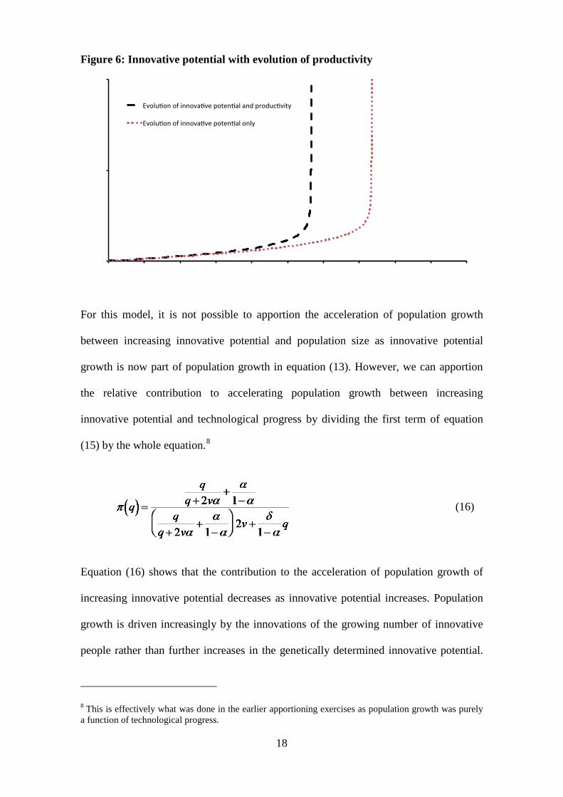
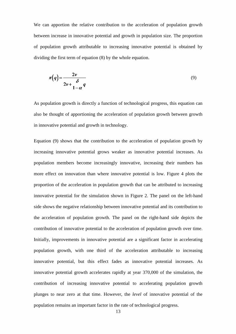
Figure 6: Innovative potential with evolution of productivity

For this model, it is not possible to apportion the acceleration of population growth

between increasing innovative potential and population size as innovative potential

growth is now part of population growth in equation (13). However, we can apportion

the relative contribution to accelerating population growth between increasing

innovative potential and technological progress by dividing the first term of equation

(15) by the whole equation.8

(16)

Equation (16) shows that the contribution to the acceleration of population growth of

increasing innovative potential decreases as innovative potential increases. Population

growth is driven increasingly by the innovations of the growing number of innovative

people rather than further increases in the genetically determined innovative potential.

8 This is effectively what was done in the earlier apportioning exercises as population growth was purely a function of technological progress.

18

Figure 7 illustrates the decline in the relative importance of increases in innovative

potential as a determinant of acceleration of population growth. At the start of the

simulation, innovative potential accounts for 42 per cent of the acceleration in

population growth. This is more than in the basic model as innovative potential

contributes to population growth through both increased innovation and productivity,

but as for the basic model, the surge in innovative potential that occurs in the simulation

precipitates a plunge in the future contribution of evolution driven population growth.

Figure 7: Relative contribution of increase in innovative potential to acceleration of population growth

6. Population dynamics

The above analysis is predicated on a steadily increasing population. However, human

evolutionary history comprises non-linear features, including population cycles and

bottlenecks. For example, genetic evidence suggests that human populations

experienced a bottleneck (or multiple bottlenecks) within the last 100,000 years that

reduced the human population to around 10,000 individuals (Harpending et al., 1993).

Under a model with no evolution, a sudden decline in population would constitute a

significant setback to technological progress. The decline in population would result in

19

a commensurate decline in idea production, and technological progress would revert to

the level experienced when the population was last of that size. If the decline in

population was caused by a technological shock, or if the population decline reduced the

level of technology available to the population through the loss of people holding ideas,

the population recovery would be no faster than the rate of population growth when the

population was last of that size. Therefore, a population suffering frequent exogenous

shocks may never escape the Malthusian state.

In a model incorporating the evolution of innovative potential, a population decline due

to a technological shock is still a setback, but technological progress and population

growth is higher than when population was last of that size as the innovative potential of

the population is now higher. This results in a faster recovery in population size and

allows for continuing acceleration of technological progress. If an evolving population

is subject to successive technological shocks, there will be successively faster recovery

from each shock, as the population will have increasingly greater innovative potential.

Figure 8 shows a simulation of four scenarios over a period of 500,000 years: a base

case for the population model without evolution, a base case for the model

incorporating human evolution, and those two scenarios being subject to exogenous

environmental shocks.9 The shock may represent a change in environmental or climatic

conditions that reduces the effective level of technology. For the two scenarios in which

exogenous technology shocks are applied, a shock at year 200,000 reduces the level of

technology to what it was at the start of the simulation (A200,000 = 1). We first assume

that innovative potential does not affect productivity, before relaxing that assumption in

later simulations.

9 The simulations in Figure 11 are generated by iterating equations (3), (4) and (5), with 1,000 years per iteration. The parameters were A0 = 1, N0 = 1, α = 0.5, 𝑦� = 1, δ = 0.001 and v = 0.0005. At t = 200,000, a shock is applied such that A200,000 = 1.

20

After the application of the technological shock, the population declines from around

1.7 in the base case without evolution and 1.8 in the base case with evolution to one in

both scenarios. The rebound in population following the shock is faster in the scenario

with human evolution. Without evolution, the shock effectively winds the clock back to

the start of the simulation. Population growth during the next 200,000 years mirrors that

for the previous 200,000 years, resulting in recovery from the shock taking that full

period. However, where innovative potential can evolve, the population recovers faster.

It takes 157,000 years for the population in the base case simulation with human

evolution to recover to the level it was at the time of the shock, compared to the 200,000

years it took to initially reach that level. The later the shock and the higher the

innovative potential of the people at the time of the shock, the faster the population will

recover.

Figure 8: Population size with environmental shocks

The recovery from shocks is even stronger where evolving innovative potential also

affects productivity. Due to the increasing productivity of the population, a higher

population is maintained at the time of the shock than in the base case model. The

population does not decrease to one because the more productive population can make

21

better use of the available technology. This is shown in Figure 9, in which a shock

reducing technology to the initial level is applied at year 200,000.10 In response to the

shock, the population size declines from 2.9 to 1.4. It then takes only 96,000 years for

the population to recover to the size it was before the shock. The robustness of the

productivity scenario to exogenous technology shocks is further demonstrated by

applying an additional shock in year 350,000. Even though 75 per cent of the population

is eliminated by this shock, the recovery in population is rapid. It takes only 64,000

years for the population to recover to its pre-shock level.

Figure 9: Population with environmental shocks and evolving productivity

7. A model with spread of mutations

An important assumption of these models is that beneficial mutations spread

immediately through the population once they arise. In reality, mutations take time to

spread through the population, and require many generations to go to fixation. The

10 The results in Figure 12 are generated by iterating equations (12), (4) and (5), with 1,000 years per iteration. The simulation parameters were A0 = 1, N0 = 1, α = 0.5, 𝑦� = 1, δ = 0.001 and v = 0.0005. At t = 200,000, a technology shock is applied such that A200,000 = 1. A second shock is applied at t = 350,000 such that A350,000 = 1.

22

delay in the spread of beneficial mutations may have significant effects on the model

outcomes, particularly for larger populations where population growth and associated

technological progress is rapid. In such cases, new mutations may initially have a

weaker effect due to their low frequency in the population. In this section, we explore

the consequences of easing the assumption of instantaneous spread of beneficial

mutations.

The time for a new mutation to spread to fixation is a function of the relative fitness of

those carrying the mutation and the size of the population. Where the mutation has a

selective advantage, the time from the emergence of a mutation to fixation can be

approximated as (Stephan et al., 1992):11

( )2 ln 2d Ns

= (17)

s is the selective advantage of the mutation. As an example, a mutation with a 5 per cent

fitness advantage (s = 0.05) in a population of one million individuals would take

approximately 580 generations or 11,600 years to spread to fixation. However, much of

this time would be related to periods where the mutation is at very low or very high

frequency along an s-shaped path. That same mutation would take only 95 generations

or 1,900 years to spread from a prevalence of one per cent to 99 per cent. Due to the

time to fixation being proportional to the log of 2N, population size has a smaller effect

on the time to fixation than the strength of selection.

11 Letting the frequency of the mutation be ωt, the change in frequency over d generations is given by:

Setting ωt = 1/2N, ωt+d = 1-1/2N and using ln(1+s) ≈ s, we can solve for d as in equation (17).

23

Despite a mutation taking d generations to spread to fixation, the effects of the new

mutation are felt through the population as soon as it arises, and it is of increasing

importance as a greater proportion of the population carries it. Letting ωt be the

prevalence of the mutation in the population at time t and Δqt an incremental change in

innovative potential due to a mutation, the contribution to technological progress from

the appearance of the mutation at time t = m to fixation at time t = d is:

(18)

If the spread of the mutation is symmetric on either side of 50 per cent, 12 then

equation (18) can be approximated as:

(19)

While this approximation underestimates the contribution of the mutation if the

population is growing, and will overstate or understate the contribution if the mutation

is recessive or dominant, it provides an approximate basis to incorporate the delay of the

mutation spreading through the population. We assume that any new mutation has no

effect on innovative potential until d/2 generations after it arises, and full effect

thereafter, as in this modified version of equation (5).

(20)

12 In a haploid population, the spread of mutations would be approximately symmetric. A recessive mutation in a diploid population (e.g. humans) increases from 50 per cent to 100 per cent more quickly than it increases from 0 per cent to 50 per cent, while dominant mutations spread more quickly from 0 per cent to 50 per cent of the population than it will from 50 per cent to fixation.

24

Substituting equations (7) and (20) into equation (8), the acceleration in population

growth is given by:

(21)

The effect of a slow spread of mutations is seen in the simulation results charted in

Figure 10. The selective advantage of the mutation is 0.001.13 The population growth is

marginally lower than would be in a simulation without the delay, and the gap between

the simulations with and without delay grows as Nt-d/2 lags further behind Nt in size.

However, the gap is relatively minor until population size grows large, as the delay in

the spread of mutations is relatively small in small populations.

Figure 10: Population size with delay in mutation moving to fixation

While the gap in population growth appears small, the delay prevents a sudden increase

in innovative potential at the time of the population explosion. As shown in Figure 11,

13 The results in Figures 10 and 11 are generated by iterating equations (3), (4) and (20), with 1,000 years per iteration. The simulation parameters were A0 = 1, N0 = 1, α = 0.5, 𝑦� = 1, δ = 0.001, v = 0.0005 and s = 0.001.

25

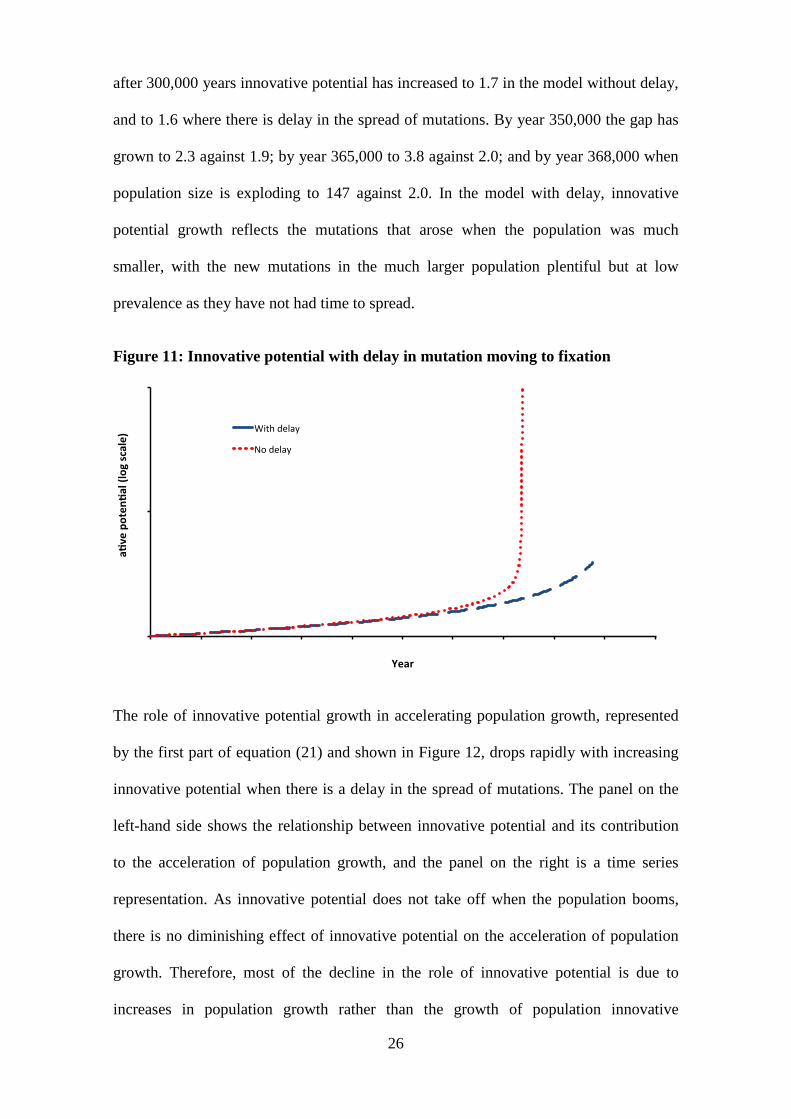
after 300,000 years innovative potential has increased to 1.7 in the model without delay,

and to 1.6 where there is delay in the spread of mutations. By year 350,000 the gap has

grown to 2.3 against 1.9; by year 365,000 to 3.8 against 2.0; and by year 368,000 when

population size is exploding to 147 against 2.0. In the model with delay, innovative

potential growth reflects the mutations that arose when the population was much

smaller, with the new mutations in the much larger population plentiful but at low

prevalence as they have not had time to spread.

Figure 11: Innovative potential with delay in mutation moving to fixation

The role of innovative potential growth in accelerating population growth, represented

by the first part of equation (21) and shown in Figure 12, drops rapidly with increasing

innovative potential when there is a delay in the spread of mutations. The panel on the

left-hand side shows the relationship between innovative potential and its contribution

to the acceleration of population growth, and the panel on the right is a time series

representation. As innovative potential does not take off when the population booms,

there is no diminishing effect of innovative potential on the acceleration of population

growth. Therefore, most of the decline in the role of innovative potential is due to

increases in population growth rather than the growth of population innovative

26

potential. Conducting the simulations with a delay in the spread of mutations for the

model that incorporates a productivity component in the production function produces a

similar pattern.

Figure 12: Relative contribution of increase in innovative potential to acceleration of population growth

8. An agent-based model

In this section, we implement the productivity-enhancing model in an agent-based

framework. In contrast to the homogeneous agents of the above models, in this agent-

based model each agent has his or her own specific level of innovative potential and

interacts with the environment as an autonomous agent.

Due to the homogeneity of the agents in the earlier models, we assumed that more

innovative people have higher fitness and that mutations spread to all agents at the same

moment. The use of an agent-based framework allows us to relax these assumptions by

endogenously incorporating these features into the model. When an agent experiences a

mutation, the spread of the mutation depends on the fitness of that agent relative to

other agents. Their fitness advantage is the result of their level of innovative potential

relative to the innovative potential of the other agents in the population. The population

27

at any point may comprise agents of multiple levels of innovative potential, with

various mutations simultaneously spreading through the population as a result of the

reproductive success of those carrying the mutations.

The population in generation t comprises Nt agents who live for one generation, with

each agent i (𝑖 ∈ 1, 2, … . ,𝑁𝑡) having innovative potential 𝑞𝑡𝑖. The innovative potential

of each agent affects their rate of idea production and the productivity with which they

utilise the available technology.

In each generation the heterogeneous agents work, producing total output Yt.

( )

1

1

1

tNi

t t ti

t t t

Y A q X

A q N X

αα

α α

−

=

−

=

=

∑ (22)

At is the level of technology available to generation t and 𝑞�𝑡 is the average innovative

potential of the agents in the population. X is the amount of land, which is normalised to

one. The parameter α is the elasticity of output with respect to labour input. The level of

per capita income is:

(23)

Technological progress is a function of the number and innovative potential of people

generating ideas:

(24)

δ is research productivity per innovation units of people.

28

As we assume that there is no ownership of or return to land, the wage per unit of

innovative potential is:

(25)

Therefore, the income of person i is:

(26)

Taking the level of per capita income where population is constant as 𝑦�, the population

will tend towards the population size that can survive off that level of income (the

Malthusian population), 𝑁�𝑡:

(27)

The expected number of children of agent i is proportional to agent i's share of total

income and the Malthusian population level for that level of total income. The realised

number of children follows a Poisson distribution.14

(28)

14 A Poisson distribution has regularly been used in the examination of the spread of beneficial mutations (Otto and Whitlock, 1997). There is some evidence that a negative binomial distribution may be more appropriate for human populations as the observed variance tends to be greater than the mean (Kojima and Kelleher, 1962), but that distribution may under-predict the number of childless agents (Waller et al., 1973). Regardless, the choice of distribution has limited effect on the simulation results.

29

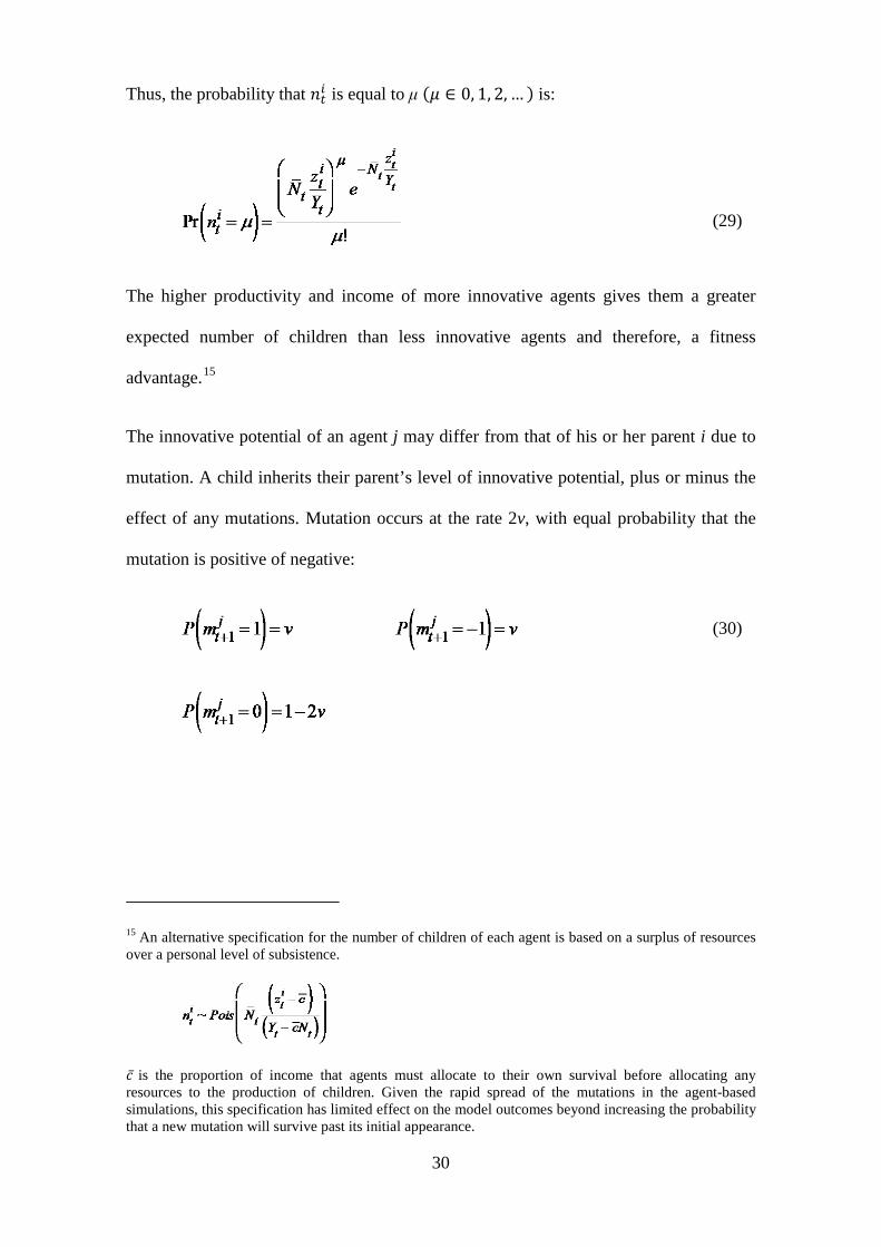
Thus, the probability that 𝑛𝑡𝑖 is equal to μ (𝜇 ∈ 0, 1, 2, … ) is:

(29)

The higher productivity and income of more innovative agents gives them a greater

expected number of children than less innovative agents and therefore, a fitness

advantage.15

The innovative potential of an agent j may differ from that of his or her parent i due to

mutation. A child inherits their parent’s level of innovative potential, plus or minus the

effect of any mutations. Mutation occurs at the rate 2v, with equal probability that the

mutation is positive of negative:

(30)

15 An alternative specification for the number of children of each agent is based on a surplus of resources over a personal level of subsistence.

𝑐̅ is the proportion of income that agents must allocate to their own survival before allocating any resources to the production of children. Given the rapid spread of the mutations in the agent-based simulations, this specification has limited effect on the model outcomes beyond increasing the probability that a new mutation will survive past its initial appearance.

30

When an agent experiences a mutation, the mutation increases or decreases innovative

potential by a factor of 1+ρ. Thus, the innovative potential of a new agent j in period t+1

is:

(31)

8.1. Simulation results

The agent-based simulations were developed in NetLogo (Wilensky, 1999), with the

agents run through the following model protocol:16

• Each agent i works and generates income 𝑧𝑡𝑖 (equation (26)).

• The agents’ activity generates technological progress, which sets the level of

technology available to the agents in the next generation (equation (24)).

• Each agent i has 𝑛𝑡𝑖 children (equation (28)).

• The innovative potential of each child j is determined (equation (31)).

• The agents from generation t die.

The parameters for the simulations are given in Table 1. All agents start at the same

level of innovative potential. The values of δ and v are lower than used in simulations

earlier in this paper, as these are rates per generation compared to rates per thousand

years used previously.

16 The code for the agent-based model is contained in the Appendix. The full NetLogo model is available for download from http://www.jasoncollins.org/downloads.

31

Table 1: Model parameters

Description Base case value

Range explored

Parameters

α Output elasticity of labour 0.5 δ Rate of innovation 10-8 10-9 to 10-7 v Mutation rate 10-6 10-7 to 10-5 ρ Mutation increment 0.1

Initial values

N0 Population 1000

𝑁�0 Malthusian population 1000

A0 Level of technology 1

𝑞0𝑖 Agent innovative potential 1

X Land 1

Figures 13 and 14 show the time paths of the population size and average innovative

potential of the population for 10 runs of the base case model. To compare the

simulation runs between the two figures, we kept the same colour code for each of the

10 runs. There is significant variation in the rate of population and innovative potential

growth despite the same parameters being used in each model run, with the timing of

chance innovative potential mutations the major determinant of the timing of the take-

off. Even where mutations occur, many mutations are eliminated at low frequencies due

to the number of children of an agent being a Poisson distribution. The number of

children of an agent may be zero even if the mutant has a higher than average expected

number of children. For example, the model runs represented by the blue and black

lines had several mutations within the first 5,000 generations, leading to an early

increase in the level of idea production per person and population size that then drives

further increases. In contrast, there were no innovation-enhancing mutations in the

model run represented by the dark green line for over 15,000 generations. This

significantly reduced the positive feedback loop between population size and innovative

potential relative to those model runs with numerous early mutations, resulting in

population differences greater than an order of magnitude at specific points. If a version

of the model were developed that relied on individual chance inventions, rather than the 32

steady accumulation of ideas as in the current implementation, the variation in the rate

of population growth between simulation runs would be even larger.

Figure 13: Population size in agent-based simulation

The step-wise nature of innovative potential growth in Figure 14 is indicative of the

rapid spread of fitness enhancing mutations when they arise and spread through the

population. As for the model in which there is a delay to the spread in mutations, the

increase in innovative potential does not match the explosive population growth at the

end of the simulation run, although it has accelerated materially.

33

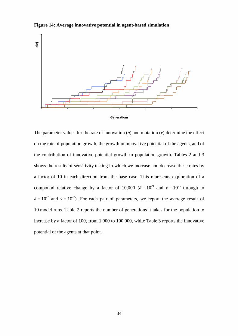
Figure 14: Average innovative potential in agent-based simulation

The parameter values for the rate of innovation (δ) and mutation (v) determine the effect

on the rate of population growth, the growth in innovative potential of the agents, and of

the contribution of innovative potential growth to population growth. Tables 2 and 3

shows the results of sensitivity testing in which we increase and decrease these rates by

a factor of 10 in each direction from the base case. This represents exploration of a

compound relative change by a factor of 10,000 (δ = 10-9 and v = 10-5 through to

δ = 10-7 and v = 10-7). For each pair of parameters, we report the average result of

10 model runs. Table 2 reports the number of generations it takes for the population to

increase by a factor of 100, from 1,000 to 100,000, while Table 3 reports the innovative

potential of the agents at that point.

34

Table 2: Sensitivity testing - Generations to 100,000 population.

Rate of innovation (δ) 10-9 5×10-9 10-8 5×10-8 10-7

Mut

atio

n ra

te (v

)

10-7 204,409 (35,859)

74,039 (13,214)

43,844 (3,633)

9,407 (631)

4,885 (182)

5×10-7 90,674 (17,616)

44,632 (7,010)

29,729 (3,056)

8,575 (681)

4,573 (243)

10-6 47,518 (12,261)

33,702 (7,172)

21,457 (3,656)

7,879 (750)

4,555 (341)

5×10-6 13,418 (1,821)

10,872 (2,619)

9,767 (1,781)

4,402 (502)

3,268 (317)

10-5 7,689 (1,478)

6,799 (716)

5,992 (1,088)

3,600 (451)

2,563 (288)

Note: Mean and standard deviation (in brackets) of 10 model runs.

Table 3: Sensitivity testing - Average innovative potential at 100,000 population.

Rate of innovation (δ) 10-9 5×10-9 10-8 5×10-8 10-7

Mut

atio

n ra

te (v

)

10-7 3.83 (0.59)

1.70 (0.27)

1.32 (0.12)

1.09 (0.08)

1.02 (0.04)

5×10-7 8.90 (0.85)

3.58 (0.64)

2.36 (0.23)

1.29 (0.10)

1.19 (0.10)

10-6 12.75 (1.01)

4.51 (0.54)

3.17 (0.40)

1.58 (0.19)

1.26 (0.10)

5×10-6 23.00 (0.85)

9.46 (0.79)

6.58 (0.50)

2.60 (0.30)

1.85 (0.12)

10-5 26.45 (1.33)

12.32 (0.83)

8.03 (0.25)

3.36 (0.27)

2.24 (0.18)

Note: Mean and standard deviation (in brackets) of 10 model runs.

The adjustment of these parameters materially affects the rate of growth and the

contribution of innovative potential to that growth. Taking a generation to be

approximately 20 years, the parameters explored can generate a 100-fold increase in

population size in 50,000 years (lower-right cell of Table 2) to four million years

(upper-left cell). Innovative potential may play almost no part in population growth

(upper-right cell of Table 3), or may increase by over 20 times (lower-left cell) being

the major driver of population growth.

35

The rate of population and innovative potential growth also varies where we use a more

general form of the equations for technological progress and the evolution of innovative

potential in which ideas or mutations may be “fished out”. However, the level of

variation is significantly below that where the rates of innovation or mutation are

adjusted. The results of sensitivity testing of more general functional forms of these

equations in the agent-based framework are contained in the Appendix.

9. Discussion

In this paper, we propose that evolutionary changes in human innovative potential can

be a complementary driver of long-term technological progress and population growth.

The concurrent increase in this potential and population growth increases the sharpness

of the take-off in technological progress and population relative to population growth

driven solely by increasing population size. The model provides scope for technological

progress to accelerate in the absence of population growth if population size is

constrained. This is particularly important where the population is subject to setbacks

that hamper long-term growth in population size, as has occurred repeatedly in human

evolutionary history. The evolution of more innovative people provides robustness to

technological shocks. Further, if human evolution selects for individuals with higher

productivity, a larger population can be maintained after a technological shock.

We also show that as the population increases in its ability to produce and use ideas,

increases in population size become a more important driver of accelerating population

growth than continued evolutionary change. This is particularly the case if there is a

delay to the spread of mutations. Increasing population size is particularly effective

where the population is already innovative, as population size has the potential to

change more quickly than mutations can spread. Indeed, the global population has

doubled over last 50 years, but any genetically based human innovative potential has

36

almost certainly not changed materially during that period. However, we did not extend

this model beyond the demographic transition and the decline in fertility of the last

200 years.

Where population size is the major driver of technological progress, there may be

potential for small populations to shrink and experience technological regress, such as

that experienced by Tasmanian aboriginals after Tasmania was isolated from the rest of

Australia by sea level rise (Diamond, 1993; Kremer, 1993). A similar possibility arises

with the evolution of the innovative potential. In a smaller population, the low level of

fitness enhancing mutation and the increased potential for the loss of beneficial

mutations through drift may reduce the ability to generate new ideas. However, the

historical presence of population bottlenecks where the human population was likely

small (in the order of 10,000 individuals) suggests that human populations have often

recovered from population shocks.

One feature of the evolution of innovative potential in this paper is that the evolution

occurs along the dimension of production of ideas, and not in relation to human ability

to transmit the ideas to other people in the population. The concept that technological

growth increases when more people create more ideas is premised on the ability of ideas

to be spread and shared between population members. While some non-human species

are recognised as engaging in learning and communication that allows the transmission

of ideas, it is limited compared to humans (Cavalli-Sforza, 1986) as they lack

mechanisms such as complex languages. Further, it is suggested that observational

learning is not a by-product of intelligence and requires specific psychological

mechanism (Boyd and Richerson, 2005). This raises the question of how and when the

human ability for the transmission of ideas evolved to allow the ideas generated by a

person to systematically spread and be used across the population. If an idea is kept by

37

and dies with an individual, or is used by only a small sub-population of humans, a

larger population will not, on average, generate more technological progress.

On that basis, the slow technological change before the emergence of behaviourally

modern humans may be partially attributable to the failure to transmit ideas across the

population. Rather than the increase in innovative potential and population size driving

increasing technological change, there may have been a step where the accumulation of

the ideas became possible, finally allowing the feedback between population,

innovation and technology to occur as humans developed the cognition and tools of

cultural learning. Before that time, the increase in population and spread to fill new

ecological niches would effectively be the result of increasing productivity, which can

capture population-supporting changes that are not the result of the spread of ideas. As

such, it is possible to develop a two-step evolutionary model with population growth

initially driven only by productivity changes. Following the evolution of a trait allowing

transmission of ideas, population size and increased innovative potential eventually

become the drivers of technological progress.

Data constraints make empirical tests of this model challenging. First, empirical tests

would require some measure of human innovation potential. A proxy such as cranial

capacity or brain size may serve this purpose, but would be a crude proxy at best. More

problematic is the degree of resolution for population data between 1 million BCE and

the present. The Deevey (1960) data used in Figure 1 contains only three data points

between one million BCE and 25,000 BCE, yet population data points would be

required for each brain size data point. Further, higher resolution population data would

likely expose the non-linear population dynamics of the human population, including

population bottlenecks. These would render a simple regression analysis of population

and innovative potential across time inappropriate. One empirical prediction of the

38

model, however, is that there would be successively faster recovery from population

shocks. For a population of the same size, an inherently more innovative population is

more resilient because it produces more ideas, with continuing evolution of that

innovative potential through time.

References

Ashraf, Q., Galor, O., 2013. The “Out of Africa” Hypothesis, Human Genetic Diversity, and Comparative Economic Development. The American Economic Review 103, 1–46.

Bailey, D.H., Geary, D.C., 2009. Hominid Brain Evolution. Human Nature 20, 67–79.

Boyd, R., Richerson, P.J., 2005. Memes: Universal Acid or a Better Mousetrap, in: The Origin and Evolution of Cultures. Oxford University Press, Oxford.

Carbonell, E., Bermúdez de Castro, J.M., Parés, J.M., Pérez-González, A., Cuenca-Bescós, G., Ollé, A., Mosquera, M., Huguet, R., van der Made, J., Rosas, A., Sala, R., Vallverdú, J., García, N., Granger, D.E., Martinón-Torres, M., Rodríguez, X.P., Stock, G.M., Vergès, J.M., Allué, E., Burjachs, F., Cáceres, I., Canals, A., Benito, A., Díez, C., Lozano, M., Mateos, A., Navazo, M., Rodríguez, J., Rosell, J., Arsuaga, J.L., 2008. The first hominin of Europe. Nature 452, 465–469.

Cavalli-Sforza, L.L., 1986. Cultural Evolution. American Zoologist 26, 845–856.

Clark, G., 2007. A Farewell to Alms: A Brief Economic History of the World. Princeton University Press, Princeton and Oxford.

Collins, J., Baer, B., Weber, E.J., 2013. Economic Growth and Evolution: Parental Preferences for Quality and Quantity of Offspring. Macroeconomic Dynamics (forthcoming).

Deevey Jr, E.S., 1960. The Human Population. Scientific American 203, 194–204.

Diamond, J., 1993. Ten thousand years of solitude 14, 48–57.

Evans, P.D., Gilbert, S.L., Mekel-Bobrov, N., Vallender, E.J., Anderson, J.R., Vaez-Azizi, L.M., Tishkoff, S.A., Hudson, R.R., Lahn, B.T., 2005. Microcephalin, a Gene Regulating Brain Size, Continues to Evolve Adaptively in Humans. Science 309, 1717–1720.

Fisher, R.A., 1930. The Genetical Theory of Natural Selection. Clarendon Press, Oxford.

Galor, O., Michalopoulos, S., 2012. Evolution and the growth process: Natural selection of entrepreneurial traits. Journal of Economic Theory 147, 759–780.

39

Galor, O., Moav, O., 2002. Natural Selection and the Origin of Economic Growth. Quarterly Journal of Economics 117, 1133–1191.

Green, R.E., Krause, J., Briggs, A.W., Maricic, T., Stenzel, U., et al., 2010. A Draft Sequence of the Neandertal Genome. Science 328, 710–722.

Haldane, J.B.S., 1927. A Mathematical Theory of Natural and Artificial Selection, Part V: Selection and Mutation. Math. Proc. Camb. Phil. Soc. 23, 838–844.

Hansson, I., Stuart, C., 1990. Malthusian Selection of Preferences. American Economic Review 80, 529–544.

Harpending, H.C., Sherry, S.T., Rogers, A.R., Stoneking, M., 1993. The Genetic Structure of Ancient Human Populations. Current Anthropology 34, 483–496.

Hawks, J., Wang, E.T., Cochran, G.M., Harpending, H.C., Moyzis, R.K., 2007. Recent acceleration of human adaptive evolution. Proceedings of the National Academy of Sciences 104, 20753–20758.

Henneberg, M., 1988. Decrease of Human Skull Size in the Holocene. Human Biology 60, 395.

Henrich, J., Gil-White, F.J., 2001. The evolution of prestige: freely conferred deference as a mechanism for enhancing the benefits of cultural transmission. Evolution and Human Behavior 22, 165–196.

Henshilwood, C.S., Marean, C.W., 2003. The Origin of Modern Human Behavior. Current Anthropology 44, 627–651.

Hoffman, M.S. (Ed.), 1991. The World Almanac. World Almanac Publishers.

Ingram, C.J.E., Mulcare, C.A., Itan, Y., Thomas, M.G., Swallow, D.M., 2008. Lactose digestion and the evolutionary genetics of lactase persistence. Hum Genet 124, 579–591.

Jones, C.I., 1995. R&D-Based Models of Economic Growth. Journal of Political Economy 103, 759–784.

Kimura, M., 1957. Some Problems of Stochastic Processes in Genetics. The Annals of Mathematical Statistics 28, 882–901.

Klein, R.G., 2000. Archeology and the evolution of human behavior. Evol. Anthropol. 9, 17–36.

Klein, R.G., Edgar, B., 2002. The Dawn of Human Culture. John Wiley & Sons, Inc., New York.

Kojima, K.-I., Kelleher, T.M., 1962. Survival of Mutant Genes. The American Naturalist 96, 329–346.

Kremer, M., 1993. Population Growth and Technological Change: One Million B.C. to 1990. Quarterly Journal of Economics 108, 681–716.

40

Kuznets, S., 1960. Population Change and Aggregate Output, in: Research, N.B. of E. (Ed.), Demographic and Economic Change in Developed Countries. UMI, pp. 340–367.

Lee, S.-H., Wolpoff, M.H., 2003. The pattern of evolution in Pleistocene human brain size. Paleobiology 29, 186–196.

Mcbrearty, S., Brooks, A.S., 2000. The revolution that wasn’t: a new interpretation of the origin of modern human behavior. Journal of Human Evolution 39, 453–563.

McEvedy, C., Jones, R., 1978. Atlas of World Population History. Viking.

Mekel-Bobrov, N., Gilbert, S.L., Evans, P.D., Vallender, E.J., Anderson, J.R., Hudson, R.R., Tishkoff, S.A., Lahn, B.T., 2005. Ongoing Adaptive Evolution of ASPM, a Brain Size Determinant in Homo sapiens. Science 309, 1720–1722.

Otto, S.P., Whitlock, M.C., 1997. The Probability of Fixation in Populations of Changing Size. Genetics 146, 723–733.

Rasmussen, M., Guo, X., Wang, Y., Lohmueller, K.E., Rasmussen, S., et al., 2011. An Aboriginal Australian Genome Reveals Separate Human Dispersals into Asia. Science 334, 94–98.

Reed, F.A., Aquadro, C.F., 2006. Mutation, selection and the future of human evolution. Trends in Genetics 22, 479–484.

Richerson, P.J., Boyd, R., Bettinger, R.L., 2001. Was Agriculture Impossible during the Pleistocene but Mandatory during the Holocene? A Climate Change Hypothesis. American Antiquity 66, 387–411.

Rightmire, G.P., 1998. Human evolution in the Middle Pleistocene: The role of Homo heidelbergensis. Evol. Anthropol. 6, 218–227.

Rightmire, G.P., 2004. Brain size and encephalization in early to Mid-Pleistocene Homo. Am. J. Phys. Anthropol. 124, 109–123.

Ruff, C.B., Trinkaus, E., Holliday, T.W., 1997. Body mass and encephalization in Pleistocene Homo. Nature 387, 173–176.

Simon, J.L., 1998. The Ultimate Resource 2. Princeton University Press, Princeton.

Spolaore, E., Wacziarg, R., 2009. The Diffusion of Development. Quarterly Journal of Economics 124, 469–529.

Stephan, W., Wiehe, T.H.E., Lenz, M.W., 1992. The effect of strongly selected substitutions on neutral polymorphism: Analytical results based on diffusion theory. Theoretical Population Biology 41, 237–254.

Tishkoff, S.A., Reed, F.A., Ranciaro, A., Voight, B.F., Babbitt, C.C., Silverman, J.S., Powell, K., Mortensen, H.M., Hirbo, J.B., Osman, M., Ibrahim, M., Omar, S.A., Lema, G., Nyambo, T.B., Ghori, J., Bumpstead, S., Pritchard, J.K., Wray, G.A., Deloukas, P., 2006. Convergent adaptation of human lactase persistence in Africa and Europe. Nat Genet 39, 31–40.

41

United Nations, 1952. United Nations Statistical Yearbook. United Nations, New York.

United Nations, 1986. United Nations Statistical Yearbook. United Nations, New York.

United Nations, 2006. United Nations Statistical Yearbook. United Nations, New York.

United Nations, 2011. United Nations Statistical Yearbook. United Nations, New York.

Voight, B.F., Kudaravalli, S., Wen, X., Pritchard, J.K., 2006. A Map of Recent Positive Selection in the Human Genome. PLoS Biol 4, e72.

Waller, J.H., Rao, B.R., Li, C.C., 1973. Heterogeneity of childless families. Biodemography and Social Biology 20, 133–138.

Wilensky, U., 1999. NetLogo. Center for Connected Learning and Computer-Based Modeling, Nortwestern University, Evanston, IL.

Zak, P.J., Park, K.W., 2002. Population Genetics and Economic Growth. Journal of Bioeconomics 4, 1–38.

42

Appendix

(For online publication only)

I. General function forms of innovation and mutation equations

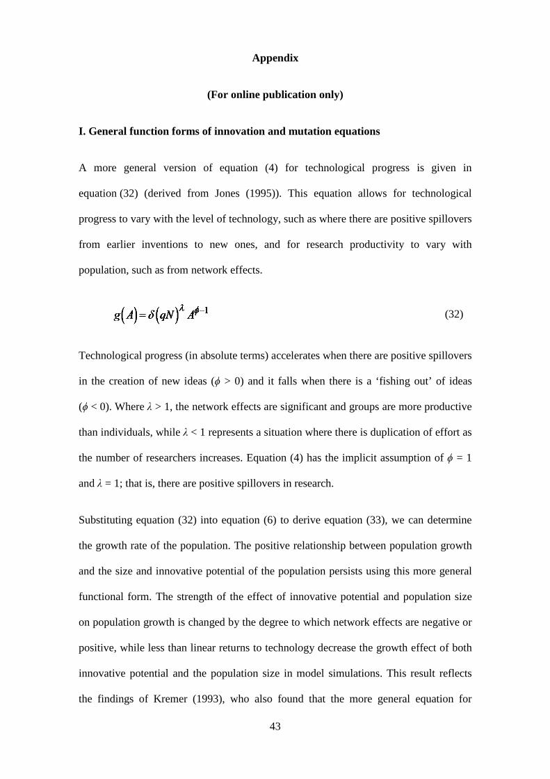
A more general version of equation (4) for technological progress is given in

equation (32) (derived from Jones (1995)). This equation allows for technological

progress to vary with the level of technology, such as where there are positive spillovers

from earlier inventions to new ones, and for research productivity to vary with

population, such as from network effects.

(32)

Technological progress (in absolute terms) accelerates when there are positive spillovers

in the creation of new ideas (ϕ > 0) and it falls when there is a ‘fishing out’ of ideas

(ϕ < 0). Where λ > 1, the network effects are significant and groups are more productive

than individuals, while λ < 1 represents a situation where there is duplication of effort as

the number of researchers increases. Equation (4) has the implicit assumption of ϕ = 1

and λ = 1; that is, there are positive spillovers in research.

Substituting equation (32) into equation (6) to derive equation (33), we can determine

the growth rate of the population. The positive relationship between population growth

and the size and innovative potential of the population persists using this more general

functional form. The strength of the effect of innovative potential and population size

on population growth is changed by the degree to which network effects are negative or

positive, while less than linear returns to technology decrease the growth effect of both

innovative potential and the population size in model simulations. This result reflects

the findings of Kremer (1993), who also found that the more general equation for

43

technological progress did not substantially change the prediction of increasing

population growth with population size.

( ) ( ) 11

g N qN Aλ φδα

−=−

(33)

Similarly, equation (5), which describes the evolution of the innovative potential of the

population, can be generalised, allowing for spillovers between mutations. There is the

possibility that the rate of “new” mutations is a function of the existing level of

mutations, as one critical mutation may provide the environment for another mutation to

have a fitness advantage, and there is the potential for depletion of certain mutations.

For example, the ability to digest lactose past childhood evolved in at least

three locations through different mutations (Ingram et al., 2008; Tishkoff et al., 2006).

Once the ability to digest lactose had evolved, new mutations that cause this trait may

not have a selective advantage relative to the existing allele.

A more general form of equation (5) where the mutation rate varies with the existing

level of innovative potential is:

(34)

There are positive returns (in absolute terms) to the existing number of fitness-

enhancing mutations when θ > 0 and decreasing when θ < 0. This contrasts with the

implicit assumption in equation (5) that there are positive returns to mutations (θ = 1).

Changing the functional form for mutations does not change equation (33).

Values of ϕ that vary from one are of interest as time series evidence from industrialised

economies suggests that the value of ϕ is less than one (Jones, 1995). While there is no

equivalent evidence that bears directly on the value of θ, it is plausible that it may also

be less than one. 44

Figures 15 and 16 show a simulation of the population with the more general functional

forms for technological progress and mutation, with ϕ = 0.4 (consistent with

one estimate of ϕ provided by Kremer (1993)), θ = 0.5 and λ = 1.17 Relative to the

simulation in Figure 2, population growth is slower as ideas and mutations are depleted.

However, the acceleration of growth remains robust and population size increases at a

greater than exponential rate.

Figure 15: Population size with general functional forms

17 The simulation is generated by iterating equations (3), (32) and (34), with 1,000 years per iteration. The simulation parameters were A0 = 1, N0 = 1, α = 0.5, 𝑦� = 1, δ = 0.001, v = 0.0005, ϕ = 0.4, θ = 0.5 and λ = 1.

45

Figure 16: Innovative potential with more general function forms

To determine the acceleration in population growth, we substitute equation (34) into

equation (8).

(35)

The acceleration in population growth is now mitigated or enhanced depending on

whether there are negative or positive network effects to innovation, and whether there

is depletion of mutations. Diminishing returns to innovation lower the acceleration in

population growth.

We can apportion the source of the acceleration of population growth between

innovative potential growth and population growth. Dividing the first term of

equation (35) by the full equation, the proportion of the acceleration in growth

attributable to increasing innovative potential is:

46

(36)

(37)

(38)

From equation (37), the relative contribution to the acceleration of population growth by

increasing innovative potential declines with innovative potential unless λ < (1-ϕ)(1-α),

which is unlikely to be the case. Equation (38) shows that the relative contribution of

increasing innovative potential to the acceleration of population growth declines with

population size under the same condition.

Figure 17 illustrates the change in the contribution of increasing innovative potential to

the acceleration of population growth for the simulation shown in Figure 15. The panel

on the left-hand side shows the underlying relationship between innovative potential

and its contribution to the acceleration of population growth, and the panel on the right

provides a time series representation. As innovative potential increases, growth in size

of the more innovative population becomes more important than continued

improvement in innovative potential.

47

Figure 17: Relative contribution of increase in innovative potential to acceleration of population growth

As was the case for the simulation of the less general functional forms, innovative

potential undergoes a rapid take-off (around year 470,000 in this case), at which point

the relative contribution of increasing innovative potential to population growth drops to

near zero.

48

II. Sensitivity testing of more general functional forms in agent-based framework

Setting the equations for technology and innovative potential growth as in equations

(39) and (40), there are less than linear returns to ideas or mutations where ϕ or θ are

below one (which is the effective value of each in the base case simulation) and

declining returns where ϕ or θ are below zero.

(39)

( )11j i i i

t t ttq q m qθ

ρ++ = + (40)

In Tables 4 and 5 we report the results of sensitivity testing for these parameters. We

calculate the number of generations for population to increase 100 fold and the

innovative potential at that point. Each result is the average of 10 model runs. Table 4

shows the number of generations for the population to increase by a factor of 100, from

1000 to 100,000, while Table 5 reports the innovative potential of the agents at that

point. These simulations show that adjusting the parameters for a more generalised form

of the technological progress and mutation equations has limited effect on the rate at

which the population grows compared to adjustment of the rates of innovation or

mutation. In the range tested, the time taken for the population to reach 100,000 varies

by less than a factor of two, while the final average agent innovative potential varies by

less than a factor of three.

49

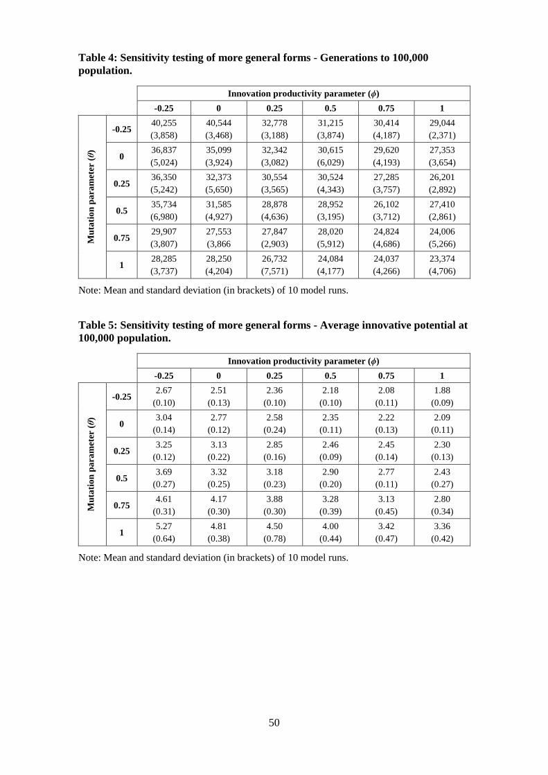
Table 4: Sensitivity testing of more general forms - Generations to 100,000 population.

Innovation productivity parameter (ϕ) -0.25 0 0.25 0.5 0.75 1

Mut

atio

n pa

ram

eter

(θ)

-0.25 40,255 (3,858)

40,544 (3,468)

32,778 (3,188)

31,215 (3,874)

30,414 (4,187)

29,044 (2,371)

0 36,837 (5,024)

35,099 (3,924)

32,342 (3,082)

30,615 (6,029)

29,620 (4,193)

27,353 (3,654)

0.25 36,350 (5,242)

32,373 (5,650)

30,554 (3,565)

30,524 (4,343)

27,285 (3,757)

26,201 (2,892)

0.5 35,734 (6,980)

31,585 (4,927)

28,878 (4,636)

28,952 (3,195)

26,102 (3,712)

27,410 (2,861)

0.75 29,907 (3,807)

27,553 (3,866

27,847 (2,903)

28,020 (5,912)

24,824 (4,686)

24,006 (5,266)

1 28,285 (3,737)

28,250 (4,204)

26,732 (7,571)

24,084 (4,177)

24,037 (4,266)

23,374 (4,706)

Note: Mean and standard deviation (in brackets) of 10 model runs.

Table 5: Sensitivity testing of more general forms - Average innovative potential at 100,000 population.

Innovation productivity parameter (ϕ) -0.25 0 0.25 0.5 0.75 1

Mut

atio

n pa

ram

eter

(θ)

-0.25 2.67

(0.10) 2.51

(0.13) 2.36

(0.10) 2.18

(0.10) 2.08

(0.11) 1.88

(0.09)

0 3.04

(0.14) 2.77

(0.12) 2.58

(0.24) 2.35

(0.11) 2.22

(0.13) 2.09

(0.11)

0.25 3.25

(0.12) 3.13

(0.22) 2.85

(0.16) 2.46

(0.09) 2.45

(0.14) 2.30

(0.13)

0.5 3.69

(0.27) 3.32

(0.25) 3.18

(0.23) 2.90

(0.20) 2.77

(0.11) 2.43

(0.27)

0.75 4.61

(0.31) 4.17

(0.30) 3.88

(0.30) 3.28

(0.39) 3.13

(0.45) 2.80

(0.34)

1 5.27

(0.64) 4.81

(0.38) 4.50

(0.78) 4.00

(0.44) 3.42

(0.47) 3.36

(0.42)

Note: Mean and standard deviation (in brackets) of 10 model runs.

50

III. Agent-based model code

The simulations in this paper were conducted using NetLogo (Wilensky, 1999), a multi-

agent programmable modelling environment. The full NetLogo model is available for

download from http://www.jasoncollins.org/downloads. Figure 18 shows a screenshot

of the NetLogo interface.

Figure 18: NetLogo interface

Program code for the agent-based simulation: globals [ A ;; technology A-old A-growth N ;; population average-q average-q-old average-q-growth w ;; wage Y ;; total income Y-old Y-growth average-z ;; average income malthusian-limit ;; population at equilbrium for a given level of technology subsistence ;; subsistence income at the Malthusian limit c ;; proportion of subsistence income that must be used on ;; self (rest available for children) alpha gamma

51

v ;; mutation rate - set by slider mutation-rate m ;; mutation increment - set by slider mutation-increment pheta phi lambda ] turtles-own [ q ;; turtle innovative potential z ;; turtle income children ;; expected number of children for a turtle age ;; use for mechanism to kill off turtles after one generation ] to setup clear-all setup-turtles set alpha labour-share set gamma innovation-rate set v mutation-rate set m mutation-increment set pheta fishing-out-mutations set phi fishing-out-A set lambda network-effects set A 1 set average-z number ^ (alpha - 1) ;; to give non-zero initial value for plot set Y average-z * number set average-q 1 ;; to give non-zero initial value for plot set subsistence number ^ (alpha - 1) ;; to set subsistence such that users can ;; select any initial number of turtles set c subsistence-self reset-ticks end to setup-turtles create-turtles number ask turtles [ setxy random-xcor random-ycor set q 1 ] end to go if N >= 100000 [ stop ;; control to stop population getting too large ] if ticks >= number-of-ticks [ stop ;; stop after a certain number of ticks ] work innovate reproduce

52

tick end to work set average-q-old average-q set average-q mean [q] of turtles set average-q-growth average-q / average-q-old - 1 set N count turtles ifelse productivity? [set w A * ((average-q * N) ^ (alpha - 1)) set malthusian-limit (subsistence / (A * average-q ^ alpha)) ^ (1 / (alpha - 1))] [set w A * (N ^ (alpha - 1)) set malthusian-limit (subsistence / A) ^ (1 / (alpha - 1))] ask turtles [ ifelse productivity? [set z q * w] [set z w] set age 1 ;; age turtles so can kill off at end of generation ] set Y-old Y set Y sum [z] of turtles set Y-growth Y / Y-old - 1 set average-z Y / N end to innovate set A-old A set A A + (A ^ phi) * (gamma * (average-q * N) ^ lambda) set A-growth A / A-old - 1 end to reproduce ask turtles [ set children malthusian-limit * (z - c * subsistence) / (Y - c * subsistence * N) hatch random-poisson children [ set age 0 setxy random-xcor random-ycor if evolution? [ ;; ability to turn off evolution to allow ;; simulation of Kremer model if (2 * v * 1000000000) > random 1000000000 [

;; set q of next generation, mutation rate 2v ifelse 1 = random 2 ;; one in two chance that mutation is either positive or negative [set q q + (m * q ^ pheta)] ;; positive mutation if random 2 = 1 [set q q - (m * q ^ pheta)] ;; negative mutation if random 2 = 0 ] ] ] if age = 1 [die] ;; kills off turtles from the last generation if q <= 0 [die] ;; kills turtles where innovative potential has mutated to zero ;; or below in no productivity simulation ] end

53

Editor, UWA Economics Discussion Papers: Ernst Juerg Weber Business School – Economics University of Western Australia 35 Sterling Hwy Crawley WA 6009 Australia Email: ecoadmin@biz.uwa.edu.au The Economics Discussion Papers are available at: 1980 – 2002: http://ecompapers.biz.uwa.edu.au/paper/PDF%20of%20Discussion%20Papers/ Since 2001: http://ideas.repec.org/s/uwa/wpaper1.html Since 2004: http://www.business.uwa.edu.au/school/disciplines/economics

ECONOMICS DISCUSSION PAPERS 2011

DP NUMBER AUTHORS TITLE

11.01 Robertson, P.E. DEEP IMPACT: CHINA AND THE WORLD ECONOMY

11.02 Kang, C. and Lee, S.H. BEING KNOWLEDGEABLE OR SOCIABLE? DIFFERENCES IN RELATIVE IMPORTANCE OF COGNITIVE AND NON-COGNITIVE SKILLS

11.03 Turkington, D. DIFFERENT CONCEPTS OF MATRIX CALCULUS

11.04 Golley, J. and Tyers, R. CONTRASTING GIANTS: DEMOGRAPHIC CHANGE AND ECONOMIC PERFORMANCE IN CHINA AND INDIA

11.05 Collins, J., Baer, B. and Weber, E.J. ECONOMIC GROWTH AND EVOLUTION: PARENTAL PREFERENCE FOR QUALITY AND QUANTITY OF OFFSPRING

11.06 Turkington, D. ON THE DIFFERENTIATION OF THE LOG LIKELIHOOD FUNCTION USING MATRIX CALCULUS

11.07 Groenewold, N. and Paterson, J.E.H. STOCK PRICES AND EXCHANGE RATES IN AUSTRALIA: ARE COMMODITY PRICES THE MISSING LINK?

11.08 Chen, A. and Groenewold, N. REDUCING REGIONAL DISPARITIES IN CHINA: IS INVESTMENT ALLOCATION POLICY EFFECTIVE?

11.09 Williams, A., Birch, E. and Hancock, P. THE IMPACT OF ON-LINE LECTURE RECORDINGS ON STUDENT PERFORMANCE

11.10 Pawley, J. and Weber, E.J. INVESTMENT AND TECHNICAL PROGRESS IN THE G7 COUNTRIES AND AUSTRALIA

11.11 Tyers, R. AN ELEMENTAL MACROECONOMIC MODEL FOR APPLIED ANALYSIS AT UNDERGRADUATE LEVEL

11.12 Clements, K.W. and Gao, G. QUALITY, QUANTITY, SPENDING AND PRICES

11.13 Tyers, R. and Zhang, Y. JAPAN’S ECONOMIC RECOVERY: INSIGHTS FROM MULTI-REGION DYNAMICS

54

11.14 McLure, M. A. C. PIGOU’S REJECTION OF PARETO’S LAW

11.15 Kristoffersen, I. THE SUBJECTIVE WELLBEING SCALE: HOW REASONABLE IS THE CARDINALITY ASSUMPTION?

11.16 Clements, K.W., Izan, H.Y. and Lan, Y. VOLATILITY AND STOCK PRICE INDEXES

11.17 Parkinson, M. SHANN MEMORIAL LECTURE 2011: SUSTAINABLE WELLBEING – AN ECONOMIC FUTURE FOR AUSTRALIA

11.18 Chen, A. and Groenewold, N. THE NATIONAL AND REGIONAL EFFECTS OF FISCAL DECENTRALISATION IN CHINA

11.19 Tyers, R. and Corbett, J. JAPAN’S ECONOMIC SLOWDOWN AND ITS GLOBAL IMPLICATIONS: A REVIEW OF THE ECONOMIC MODELLING

11.20 Wu, Y. GAS MARKET INTEGRATION: GLOBAL TRENDS AND IMPLICATIONS FOR THE EAS REGION

11.21 Fu, D., Wu, Y. and Tang, Y. DOES INNOVATION MATTER FOR CHINESE HIGH-TECH EXPORTS? A FIRM-LEVEL ANALYSIS

11.22 Fu, D. and Wu, Y. EXPORT WAGE PREMIUM IN CHINA’S MANUFACTURING SECTOR: A FIRM LEVEL ANALYSIS

11.23 Li, B. and Zhang, J. SUBSIDIES IN AN ECONOMY WITH ENDOGENOUS CYCLES OVER NEOCLASSICAL INVESTMENT AND NEO-SCHUMPETERIAN INNOVATION REGIMES

11.24 Krey, B., Widmer, P.K. and Zweifel, P. EFFICIENT PROVISION OF ELECTRICITY FOR THE UNITED STATES AND SWITZERLAND

11.25 Wu, Y. ENERGY INTENSITY AND ITS DETERMINANTS IN CHINA’S REGIONAL ECONOMIES

55

ECONOMICS DISCUSSION PAPERS 2012

DP NUMBER AUTHORS TITLE

12.01 Clements, K.W., Gao, G., and Simpson, T.

DISPARITIES IN INCOMES AND PRICES INTERNATIONALLY

12.02 Tyers, R. THE RISE AND ROBUSTNESS OF ECONOMIC FREEDOM IN CHINA

12.03 Golley, J. and Tyers, R. DEMOGRAPHIC DIVIDENDS, DEPENDENCIES AND ECONOMIC GROWTH IN CHINA AND INDIA

12.04 Tyers, R. LOOKING INWARD FOR GROWTH

12.05 Knight, K. and McLure, M. THE ELUSIVE ARTHUR PIGOU

12.06 McLure, M. ONE HUNDRED YEARS FROM TODAY: A. C. PIGOU’S WEALTH AND WELFARE

12.07 Khuu, A. and Weber, E.J. HOW AUSTRALIAN FARMERS DEAL WITH RISK

12.08 Chen, M. and Clements, K.W. PATTERNS IN WORLD METALS PRICES

12.09 Clements, K.W. UWA ECONOMICS HONOURS

12.10 Golley, J. and Tyers, R. CHINA’S GENDER IMBALANCE AND ITS ECONOMIC PERFORMANCE

12.11 Weber, E.J. AUSTRALIAN FISCAL POLICY IN THE AFTERMATH OF THE GLOBAL FINANCIAL CRISIS

12.12 Hartley, P.R. and Medlock III, K.B. CHANGES IN THE OPERATIONAL EFFICIENCY OF NATIONAL OIL COMPANIES

12.13 Li, L. HOW MUCH ARE RESOURCE PROJECTS WORTH? A CAPITAL MARKET PERSPECTIVE

12.14 Chen, A. and Groenewold, N. THE REGIONAL ECONOMIC EFFECTS OF A REDUCTION IN CARBON EMISSIONS AND AN EVALUATION OF OFFSETTING POLICIES IN CHINA

12.15 Collins, J., Baer, B. and Weber, E.J. SEXUAL SELECTION, CONSPICUOUS CONSUMPTION AND ECONOMIC GROWTH

12.16 Wu, Y. TRENDS AND PROSPECTS IN CHINA’S R&D SECTOR

12.17 Cheong, T.S. and Wu, Y. INTRA-PROVINCIAL INEQUALITY IN CHINA: AN ANALYSIS OF COUNTY-LEVEL DATA

12.18 Cheong, T.S. THE PATTERNS OF REGIONAL INEQUALITY IN CHINA

12.19 Wu, Y. ELECTRICITY MARKET INTEGRATION: GLOBAL TRENDS AND IMPLICATIONS FOR THE EAS REGION

12.20 Knight, K. EXEGESIS OF DIGITAL TEXT FROM THE HISTORY OF ECONOMIC THOUGHT: A COMPARATIVE EXPLORATORY TEST

12.21 Chatterjee, I. COSTLY REPORTING, EX-POST MONITORING, AND COMMERCIAL PIRACY: A GAME THEORETIC ANALYSIS

12.22 Pen, S.E. QUALITY-CONSTANT ILLICIT DRUG PRICES

12.23 Cheong, T.S. and Wu, Y. REGIONAL DISPARITY, TRANSITIONAL DYNAMICS AND CONVERGENCE IN CHINA

56

12.24 Ezzati, P. FINANCIAL MARKETS INTEGRATION OF IRAN WITHIN THE MIDDLE EAST AND WITH THE REST OF THE WORLD

12.25 Kwan, F., Wu, Y. and Zhuo, S. RE-EXAMINATION OF THE SURPLUS AGRICULTURAL LABOUR IN CHINA

12.26 Wu, Y. R&D BEHAVIOUR IN CHINESE FIRMS

12.27 Tang, S.H.K. and Yung, L.C.W. MAIDS OR MENTORS? THE EFFECTS OF LIVE-IN FOREIGN DOMESTIC WORKERS ON SCHOOL CHILDREN’S EDUCATIONAL ACHIEVEMENT IN HONG KONG

12.28 Groenewold, N. AUSTRALIA AND THE GFC: SAVED BY ASTUTE FISCAL POLICY?

ECONOMICS DISCUSSION PAPERS 2013

DP NUMBER AUTHORS TITLE

13.01 Chen, M., Clements, K.W. and Gao, G.

THREE FACTS ABOUT WORLD METAL PRICES

13.02 Collins, J. and Richards, O. EVOLUTION, FERTILITY AND THE AGEING POPULATION

13.03 Clements, K., Genberg, H., Harberger, A., Lothian, J., Mundell, R., Sonnenschein, H. and Tolley, G.

LARRY SJAASTAD, 1934-2012

13.04 Robitaille, M.C. and Chatterjee, I. MOTHERS-IN-LAW AND SON PREFERENCE IN INDIA

13.05 Clements, K.W. and Izan, I.H.Y. REPORT ON THE 25TH PHD CONFERENCE IN ECONOMICS AND BUSINESS

13.06 Walker, A. and Tyers, R. QUANTIFYING AUSTRALIA’S “THREE SPEED” BOOM

13.07 Yu, F. and Wu, Y. PATENT EXAMINATION AND DISGUISED PROTECTION

13.08 Yu, F. and Wu, Y. PATENT CITATIONS AND KNOWLEDGE SPILLOVERS: AN ANALYSIS OF CHINESE PATENTS REGISTER IN THE US

13.09 Chatterjee, I. and Saha, B. BARGAINING DELEGATION IN MONOPOLY

13.10 Cheong, T.S. and Wu, Y. GLOBALIZATION AND REGIONAL INEQUALITY IN CHINA

13.11 Cheong, T.S. and Wu, Y. INEQUALITY AND CRIME RATES IN CHINA

13.12 Robertson, P.E. and Ye, L. ON THE EXISTENCE OF A MIDDLE INCOME TRAP

13.13 Robertson, P.E. THE GLOBAL IMPACT OF CHINA’S GROWTH

13.14 Hanaki, N., Jacquemet, N., Luchini, S., and Zylbersztejn, A.

BOUNDED RATIONALITY AND STRATEGIC UNCERTAINTY IN A SIMPLE DOMINANCE SOLVABLE GAME

13.15 Okatch, Z., Siddique, A. and Rammohan, A.

DETERMINANTS OF INCOME INEQUALITY IN BOTSWANA

57

13.16 Clements, K.W. and Gao, G. A MULTI-MARKET APPROACH TO MEASURING THE CYCLE

13.17 Chatterjee, I. and Ray, R. THE ROLE OF INSTITUTIONS IN THE INCIDENCE OF CRIME AND CORRUPTION

13.18 Fu, D. and Wu, Y. EXPORT SURVIVAL PATTERN AND DETERMINANTS OF CHINESE MANUFACTURING FIRMS

13.19 Shi, X., Wu, Y. and Zhao, D. KNOWLEDGE INTENSIVE BUSINESS SERVICES AND THEIR IMPACT ON INNOVATION IN CHINA

13.20 Tyers, R., Zhang, Y. and Cheong, T.S.

CHINA’S SAVING AND GLOBAL ECONOMIC PERFORMANCE

13.21 Collins, J., Baer, B. and Weber, E.J. POPULATION, TECHNOLOGICAL PROGRESS AND THE EVOLUTION OF INNOVATIVE POTENTIAL

13.22 Hartley, P.R. THE FUTURE OF LONG-TERM LNG CONTRACTS

13.23 Tyers, R. A SIMPLE MODEL TO STUDY GLOBAL MACROECONOMIC INTERDEPENDENCE

13.24 McLure, M. REFLECTIONS ON THE QUANTITY THEORY: PIGOU IN 1917 AND PARETO IN 1920-21

58